Stochastic Effects in Hybrid Inflation

Abstract

Hybrid inflation is a two-field model where inflation ends due to an instability. In the neighborhood of the instability point, the potential is very flat and the quantum fluctuations dominate over the classical motion of the inflaton and waterfall fields. In this article, we study this regime in the framework of stochastic inflation. We numerically solve the two coupled Langevin equations controlling the evolution of the fields and compute the probability distributions of the total number of e-folds and of the inflation exit point. Then, we discuss the physical consequences of our results, in particular the question of how the quantum diffusion can affect the observable predictions of hybrid inflation.

I Introduction

Inflation is the leading scenario among the models attempting to describe the physical conditions that prevailed in the very early Universe. It consists in a phase of accelerated expansion which naturally solves the problems of the hot big bang theory Starobinsky (1980); Guth (1981); Linde (1982); Albrecht and Steinhardt (1982); Linde (1983) (for reviews, see Refs. Martin (2004, 2005, 2008)). In addition, it predicts an almost scale invariant power spectrum for the primordial cosmological fluctuations, the tiny deviations from scale invariance being related to the microphysics of inflation Mukhanov and Chibisov (1981, 1982); Hawking (1982); Starobinsky (1982); Guth and Pi (1982); Bardeen et al. (1983). As is well known, this prediction turns out to be fully consistent with different types of astrophysical observationsm among which is the measurement of the cosmic microwave background radiation (CMBR) anisotropies Martin and Ringeval (2006); Lorenz et al. (2008a, b); Martin and Ringeval (2010); Martin et al. (2011).

Inflation is usually driven by one or many scalar fields. In the context of general relativity, this represents the simplest mechanism to obtain the negative pressure necessary to produce an accelerated expansion. However, the physical nature of those scalar fields is presently unknown, and many different inflationary models have been suggested. The reason for such a situation originates from the fact that inflation is a high energy phenomenon. Indeed, the energy scale of inflation is somewhere between the TeV scale and the grand unified theory scale Martin and Ringeval (2006). At those scales, particle physics remains elusive, and for a consequence, there is presently a large variety of different inflationary scenarios.

However, given the extensions of the standard model of particle physics, notably those based on supersymmetry and supergravity, it is clear that some models appear to be more motivated and more generic than others. In particular, this is the case of hybrid inflation Linde (1994); Copeland et al. (1994), which can be realized in various ways in the context of supersymmetry, see for instance the scenarios named $F$-term inflation and $D$-term inflation (among others) Halyo (1996); Binetruy and Dvali (1996); Dvali et al. (1994); Kallosh and Linde (2003). Hybrid inflation is a two-field model such that inflation occurs along a valley in the field space and ends by tachyonic instability along the so-called waterfall field direction. Hybrid inflation is known to lead to a blue spectrum for the fluctuations, a prediction which appears to be disfavored by the most recent observations Martin and Ringeval (2006). However, it was shown recently Clesse and Rocher (2009); Clesse (2011); Abolhasani et al. (2011a) that, in some regions of the parameter space, a significant number of e-folds can occur in the waterfall regime. In this case, it was also demonstrated that the spectral index becomes red, which therefore implies that the model is in fact totally compatible with the data Clesse and Rocher (2009); Clesse (2011).

In the context of inflation, another interesting question is the role played by the quantum corrections Vilenkin (1983); Starobinsky (1986); Goncharov et al. (1987); Nambu and Sasaki (1988, 1989); Kandrup (1989); Nakao et al. (1988); Nambu (1989); Mollerach et al. (1991); Linde et al. (1994); Starobinsky and Yokoyama (1994). Various works have shown that they can have a crucial impact on the inflationary dynamics. This is, for instance, the case for large field inflation if one starts inflation high enough in the potential. In this case, the quantum kicks undergone by the field can be so important that the field climbs its potential instead of rolling down it as should be the case according to the classical equations of motion. In such a situation, it is likely that one enters into a regime of eternal inflation Linde (1986a, b); Goncharov et al. (1987).

Hybrid inflation is also a model where one expects the quantum corrections to be very important. It should be the case high in the inflationary valley but also around the critical point where the tachyonic instability is triggered Garcia-Bellido et al. (1996); Clesse and Rocher (2009); Clesse (2011). The goal of this article is to investigate this last question in detail. In particular, we are interested in whether the quantum effects can significantly modify the classical dynamics and affect the observational predictions of the model.

In order to carry out our study, we use the stochastic inflation formalism Starobinsky (1986); Nambu and Sasaki (1988, 1989); Kandrup (1989); Nakao et al. (1988); Nambu (1989); Mollerach et al. (1991); Linde et al. (1994); Starobinsky and Yokoyama (1994); Martin and Musso (2006a, b). It consists in modeling the quantum effects by a stochastic white noise. As a consequence, the equation describing the motion of the fields becomes a Langevin equation. As mentioned previously, hybrid inflation is a genuine two-field model, which implies that one has to deal with two coupled Langevin equations. Solving this system is a very complicated task, even if a perturbative expansion is used, as usually done in the context of single field inflation. This is the reason why, in this article, we use a numerical approach. This allows us to compute various interesting quantities such as the probability density function for the number of e-folds or for the location in field space of the end of inflation.

This article is organized as follows. In the next section, Sec. II, we review in some detail the classical behavior of the inflaton and waterfall fields. This allows us to clearly identify the region in the parameter space where a significant number of e-folds can occur during the waterfall regime. This also permits a comparison between the classical and stochastic dynamics. In Sec. III we numerically solve the two coupled Langevin equations that control the behavior of the two fields. We then use this result to compute various probability density functions, in particular, that of the number of e-folds and of the inflation exit point. Finally, in Sec. IV we summarize our main results and present our conclusions.

II Classical regimes

There exist many ways to realize hybrid inflation. In this article, for simplicity, we focus on the first version studied in Ref. Linde (1994); see also Ref. Green and Mazumdar (2002). In this case, the potential in the field space $\left(\phi,\psi\right)$, where $\phi$ is the inflaton and $\psi$ the waterfall field, is given by the following expression:

$$V\left(\phi,\psi\right)=\Lambda^{4}\left[\left(1-\frac{\psi^{2}}{M^{2}}\right)^{2}+\frac{\phi^{2}}{\mu^{2}}+2\frac{\phi^{2}\psi^{2}}{\phi_{\mathrm{c}}^{2}M^{2}}\right].$$ (1)

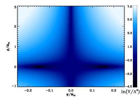
It contains four parameters (of dimension one), $\Lambda$, $M$, $\mu$, and $\phi_{\mathrm{c}}$. The scale $\Lambda$ is fixed by the Cosmic Background Explorer (COBE) normalization (the other parameters being fixed). The true minimums of the potential are located at $\phi=0$ and $\psi=\pm M$, while the instability point is given by $\phi=\phi_{\mathrm{c}}$, $\psi=0$. Along the inflationary valley, $\psi=0$, the potential reduces to $\Lambda^{4}\left[1+(\phi/\mu)^{2}\right]$ which shows that, in this regime, inflation cannot end by violation of the slow-roll conditions. The full hybrid inflation potential is shown in Fig. 1 where the inflationary valley is clearly visible.

Figure 1: Potential of hybrid inflation in the $\left(\phi,\psi\right)$ plane. The values of the parameters are $\mu=3190.4\,M_{\scriptscriptstyle{\mathrm{Pl}}}$, $M=\phi_{\mathrm{c}}=0.1503\,M_{\scriptscriptstyle{\mathrm{Pl}}}$, with $M_{\scriptscriptstyle{\mathrm{Pl}}}$ being the reduced Planck mass.

In this section we study the classical behaviors of the inflaton and waterfall fields. The slow-roll equations controlling the evolution of the fields can be expressed as

$$3H^{2}\frac{\mathrm{d}\phi}{\mathrm{d}N} = -\frac{2\Lambda^{4}\phi}{\mu^{2}}\left(1+\frac{2\psi^{2}\mu^{2}}{\phi_{\mathrm{c}}^{2}M^{2}}\right)\,,$$ (2)

$$3H^{2}\frac{\mathrm{d}\psi}{\mathrm{d}N} = -\frac{4\Lambda^{4}}{M^{2}}\psi\left(\frac{\phi^{2}-\phi_{\mathrm{c}}^{2}}{\phi_{\mathrm{c}}^{2}}+\frac{\psi^{2}}{M^{2}}\right)\,,$$ (3)

where $H=\dot{a}/a$ is the Hubble parameter, $a(t)$ being the Friedman-Lemaitre-Robertson-Walker (FLRW) scale factor and a dot denoting a derivative with respect to cosmic time. The quantity $N$ is the number of e-folds, $N\equiv\ln(a/a_{\mathrm{i}})$, where $a_{\mathrm{i}}$ is the scale factor at the beginning of inflation.

Figure 2: Exact numerical solution for the inflaton (left panel, solid blue line) and waterfall (right panel, solid blue line) fields in the inflationary valley . The red dotted lines represent the analytical solution and it is obvious that the approximation is very good. The damped oscillations of the waterfall field along the inflationary valley are clearly visible. The WKB analytical formula given by Eq. (17) is a very good approximation to the exact numerical solution.

In order to study the classical dynamics, it is interesting to calculate the slow-roll parameters. The hierarchy defined from the potential Stewart and Lyth (1993); Liddle et al. (1994); Groot Nibbelink and van Tent (2002); Easther and Giblin (2005) is given by the following expressions:

$$\epsilon_{\phi} = \frac{2\phi^{2}M_{\scriptscriptstyle{\mathrm{Pl}}}^{2}}{\mu^{4}}\left(1+\frac{2\psi^{2}\mu^{2}}{\phi_{\mathrm{c}}^{2}M^{2}}\right)\,,$$ (4)

$$\epsilon_{\psi} = \frac{8M_{\scriptscriptstyle{\mathrm{Pl}}}^{2}\psi^{2}}{M^{4}}\left(\frac{\phi^{2}-\phi_{\mathrm{c}}^{2}}{\phi_{\mathrm{c}}^{2}}+\frac{\psi^{2}}{M^{2}}\right)\,,$$ (5)

$$\eta_{\phi\phi} = \frac{2M_{\scriptscriptstyle{\mathrm{Pl}}}^{2}}{\mu^{2}}\left(1+\frac{2\mu^{2}\psi^{2}}{\phi_{\mathrm{c}}^{2}M^{2}}\right)\,,$$ (6)

$$\eta_{\phi\psi} = \frac{8M_{\scriptscriptstyle{\mathrm{Pl}}}^{2}\phi\psi}{\phi_{\mathrm{c}}^{2}M^{2}}\,,$$ (7)

$$\eta_{\psi\psi} = \frac{4M_{\scriptscriptstyle{\mathrm{Pl}}}^{2}}{M^{2}}\left(\frac{\phi^{2}-\phi_{\mathrm{c}}^{2}}{\phi_{\mathrm{c}}^{2}}+3\frac{\psi^{2}}{M^{2}}\right)\,.$$ (8)

On the other hand, the hierarchy defined from the Hubble parameter, the so-called Hubble flow parameters Schwarz et al. (2001); Leach et al. (2002), can be expressed as

$$\epsilon_{n+1}\equiv\frac{{\rm d}\ln|\epsilon_{n}|}{{\rm d}N},$$ (9)

where $\epsilon_{0}=H_{\rm i}/H(N)$. The above expression implies that having inflation is strictly equivalent to $\epsilon_{1}<1$, where $\epsilon_{1}=-\dot{H}/H^{2}$. Obviously, the two hierarchies are related by simple expressions. In particular, the first horizon flow parameter is

$$\epsilon_{1}\simeq\epsilon_{\phi}+\epsilon_{\psi},$$ (10)

where $\epsilon_{\phi}$ and $\epsilon_{\psi}$ have been defined before.

Having specified the notation, we now turn to the choice of the free parameters controlling the shape of the inflationary potential.

II.1 Physical Priors

It is usually assumed that hybrid inflation occurs in the vacuum dominated regime, for which $\phi\ll\mu$ and $\psi\ll M$. In this paper we also assume that this is the case. In any case, otherwise, hybrid inflation in the valley would be equivalent to a large field model, which is not the regime of interest here. For simplicity, in order to reduce the number of free parameters, and as also motivated by the supersymmetric version of the model, we take $\phi_{\mathrm{c}}\simeq M$. Notice that this assumption does not imply a loss of generality, as we could easily relax it without drastically modifying the results obtained in this paper. Finally, in order for inflation to proceed for small values of the fields (compared to the Planck mass), one can consider that $\phi_{\mathrm{c}},M\ll M_{\scriptscriptstyle{\mathrm{Pl}}}$, $M_{\scriptscriptstyle{\mathrm{Pl}}}$ being the reduced Planck mass.

In the valley and in the $\phi/\mu\ll 1$ limit, the slow-roll parameters $\epsilon_{1}$ and $\epsilon_{2}$ read

$$\epsilon_{1}\left(\phi,\psi=0\right) \simeq 2\frac{M_{\scriptscriptstyle{\mathrm{Pl}}}^{2}}{\mu^{2}}\frac{\phi^{2}}{\mu^{2}}\,,$$ (11)

$$\epsilon_{2}\left(\phi,\psi=0\right) \simeq 4\frac{M_{\scriptscriptstyle{\mathrm{Pl}}}^{2}}{\mu^{2}}\,.$$ (12)

Therefore, for the slow-roll approximation to be satisfied, these two parameters have to be much smaller than $1$, which implies that $\mu\gg M_{\scriptscriptstyle{\mathrm{Pl}}}$.

In the next subsection we study the behavior of the two fields during the first phase of evolution, namely when the inflaton field is moving along the valley.

II.2 The Inflationary Valley

The question of the initial conditions in hybrid inflation is a very interesting and non-trivial question. It has been studied in detail in Refs. Clesse (2010a, b); Clesse et al. (2009); Clesse and Rocher (2009). Here, we simply argue that starting in the valley can be reasonably justified even if more complicated regimes can be found; see Ref. Clesse (2010b). Indeed, if inflation starts beyond the critical line $\phi=\phi_{\mathrm{c}}$, the system very quickly reaches the region where $\psi/M\ll 1$. In this regime, where the inflaton field is driving inflation, the slow-roll equation of motion for $\phi$ can be integrated, leading to

$$N=\frac{1}{4}\frac{\mu^{2}}{M_{\scriptscriptstyle{\mathrm{Pl}}}^{2}}\left[\frac{\phi_{\mathrm{in}}^{2}}{\mu^{2}}-\frac{\phi^{2}}{\mu^{2}}-2\ln\left(\frac{\phi}{\phi_{\mathrm{in}}}\right)\right]\ ,$$ (13)

where $\phi_{\mathrm{in}}$ denotes the initial value of the inflaton field. This relation can be inverted, and one obtains Martin and Ringeval (2006)

$$\frac{\phi}{\mu}=\left[W_{0}\left(\frac{\phi_{\mathrm{in}}^{2}}{\mu^{2}}\mathrm{e}^{\phi_{\mathrm{in}}^{2}/\mu^{2}-4M_{\scriptscriptstyle{\mathrm{Pl}}}^{2}N/\mu^{2}}\right)\right]^{1/2}\ ,$$ (14)

where $W_{0}$ denotes the $0$-branch of the Lambert function. In the $\phi/\mu\ll 1$ limit, this formula simply reads

$$\phi=\phi_{\mathrm{in}}\exp\left(-2\frac{M_{\scriptscriptstyle{\mathrm{Pl}}}^{2}}{\mu^{2}}N\right)\ .$$ (15)

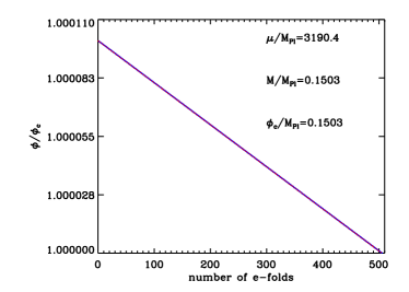
This last expression is compared with an exact numerical integration of the full equations of motion in Fig. 2 (left panel), where it is shown that this is indeed an excellent approximation. Moreover, this allows us to calculate the number of e-folds “generated” in the valley, which reads

$$N_{\mathrm{c}}=\frac{\mu^{2}}{2M_{\scriptscriptstyle{\mathrm{Pl}}}^{2}}\ln\left(\frac{\phi_{\mathrm{in}}}{\phi_{\mathrm{c}}}\right)\,.$$ (16)

Clearly, this number is large because $\mu\gg M_{\scriptscriptstyle{\mathrm{Pl}}}$.

Figure 3: Exact numerical solution for the waterfall field (solid blue line) in the inflationary valley after the oscillatory regime. The red dotted line represents the analytical solution, and it is obvious that the approximation is very good.

Let us now study the behavior of the waterfall field in the vicinity of the valley, when $\psi/M\ll 1$. Since $\psi$ undergoes damped oscillations in this regime, it is clear that the slow-roll approximation cannot be used. On the other hand, since $\psi$ oscillates much faster than $\phi$ moves, the Wentzel-Kramers-Brillouin (WKB) approximation can be used to describe this regime. The solution can be expressed as

$$\psi = \psi_{\mathrm{in}}\frac{{\rm e}^{-3N/2}}{\sqrt{2\omega(N)}}\left[C_{1}{\rm e}^{I\left(N\right)}+C_{2}{\rm e}^{-I\left(N\right)}\right],$$ (17)

where $\psi_{\mathrm{in}}$ is the initial value of the waterfall field, and where $I\left(N\right)$ is defined by the following expression (an unimportant sign has been ignored):

$$I\left(N\right) \equiv i\int\omega(n){\rm d}n,$$ (18)

$$= \frac{3}{2}\int_{0}^{N}\sqrt{1-\frac{16}{3}\frac{M_{\scriptscriptstyle{\mathrm{Pl}}}^{2}}{M^{2}}\frac{\phi^{2}/\phi_{\mathrm{c}}^{2}-1}{1+\phi^{2}/\mu^{2}}}\,\mathrm{d}n,$$ (19)

and where $C_{1}$ and $C_{2}$ are integration constants. The validity of the WKB approximation can be checked by estimating the following quantity, $({\rm d}\omega/{\rm d}N)/\omega\simeq{\cal O}(1)M_{\scriptscriptstyle{\mathrm{Pl}}}^{2}/\mu^{2}\ll 1$. From the above expression one notices that oscillations in the $\psi$ direction occur in the regime

$$\frac{16}{3}\frac{M_{\scriptscriptstyle{\mathrm{Pl}}}^{2}}{M^{2}}\frac{\phi^{2}/\phi_{\mathrm{c}}^{2}-1}{1+\phi^{2}/\mu^{2}}>1\,,$$ (20)

that is to say, in the region

$$\frac{\phi}{\phi_{\mathrm{c}}}>1+\frac{3}{32}\frac{M^{2}}{M_{\scriptscriptstyle{\mathrm{Pl}}}^{2}}.$$ (21)

Since $M\ll M_{\scriptscriptstyle{\mathrm{Pl}}}$, we see that the field oscillates almost all the time before the critical point is met. In fact, it turns out that the integral $I(N)$ can be performed. One finds

$$I(N) \simeq -\sqrt{3}\frac{M_{\scriptscriptstyle{\mathrm{Pl}}}}{M}\frac{\mu^{2}}{M_{\scriptscriptstyle{\mathrm{Pl}}}^{2}}\Biggl{[}\sqrt{\frac{\phi^{2}}{\phi_{\mathrm{c}}^{2}}-1}-\arctan\left(\sqrt{\frac{\phi^{2}}{\phi_{\mathrm{c}}^{2}}-1}\right)$$ (22)

$$- \sqrt{\frac{\phi_{\mathrm{in}}^{2}}{\phi_{\mathrm{c}}^{2}}-1}+\arctan\left(\sqrt{\frac{\phi^{2}_{\mathrm{in}}}{\phi_{\mathrm{c}}^{2}}-1}\right)\Biggr{]}.$$

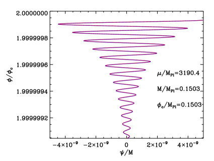
This solution is compared with the exact numerical solution in Fig. 2 (right panel). Clearly, the approximation is excellent.

When the condition (21) is not satisfied, $I(N)\simeq\pm 3N/2+\cdots$ and the oscillations stop. Since the gradients become small, this time, one can use the slow-roll approximation in order to describe the motion of $\psi$. Notice that, since $M$ is small (in Planck units), the above-mentioned regime occurs for a very small range of values for $\phi$. However, a large number of e-folds $\propto\mu^{2}M^{2}/M_{\scriptscriptstyle{\mathrm{Pl}}}^{4}$ can be produced during this phase. The slow-roll equation of motion for $\psi$ can be straightforwardly integrated and gives

$$\psi=\psi_{\mathrm{in}}\exp\left[4\frac{M_{\scriptscriptstyle{\mathrm{Pl}}}^{2}}{M^{2}}\int_{0}^{N}\frac{1-\phi^{2}\left(n\right)/\phi_{\mathrm{c}}^{2}}{1+\phi^{2}\left(n\right)/\mu^{2}}\,\mathrm{d}n\right]\ ,$$ (23)

where $\phi\left(n\right)$ is given by Eq. (14). Since $\phi>\phi_{\mathrm{c}}$ in the valley, $\psi$ decreases with $N$ and obviously remains in the $\psi\ll M$ region. If one uses the fact that $\phi\ll\mu$, then the integral in the above formula can be performed exactly. Upon using Eq. (15), one obtains

$$\psi = \psi_{\mathrm{in}}\exp\left[4\frac{M_{\scriptscriptstyle{\mathrm{Pl}}}^{2}}{M^{2}}N-\frac{\phi_{\mathrm{in}}^{2}}{\phi_{\mathrm{c}}^{2}}\frac{\mu^{2}}{M^{2}}\right.$$ (24)

$$+\left.\frac{\phi_{\mathrm{in}}^{2}}{\phi_{\mathrm{c}}^{2}}\frac{\mu^{2}}{M^{2}}\exp\left(-4\frac{M_{\scriptscriptstyle{\mathrm{Pl}}}^{2}}{\mu^{2}}N\right)\right]$$

$$\simeq \psi_{\mathrm{in}}\exp\left[-4\frac{M_{\scriptscriptstyle{\mathrm{Pl}}}^{2}}{M^{2}}\left(\frac{\phi_{\mathrm{in}}}{\phi_{\mathrm{c}}}-1\right)N\right]\,,$$

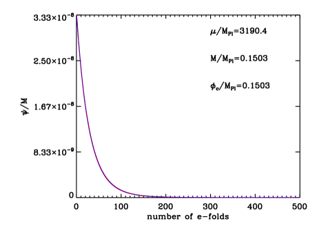
where, in the last equation, we have used the fact that $\mu\gg M_{\scriptscriptstyle{\mathrm{Pl}}}$. In that case, one concludes that $\psi$ is exponentially damped after the oscillations have stopped and before the critical point is reached. To our knowledge, this regime was not considered before. The above expression is compared with an exact numerical integration of the full equations of motion in Fig. 3. As one can notice, the agreement between the exact numerical solution and the analytical approximated expression is excellent. The previous formula also allows us to calculate the classical value of $\psi$ when the system reaches the critical point. It is given by

$$\psi_{\mathrm{c}}=\psi_{\mathrm{in}}\exp\left[-2\frac{\mu^{2}}{M^{2}}\left(\frac{\phi_{\mathrm{in}}}{\phi_{\mathrm{c}}}-1\right)\ln\left(\frac{\phi_{\mathrm{in}}}{\phi_{\mathrm{c}}}\right)\right]\,.$$ (25)

In practice, this value is always extremely small, thanks to the fact that $\mu\gg M_{\scriptscriptstyle{\mathrm{Pl}}}^{2}$ and, as was noticed in Refs. Garcia-Bellido et al. (1996); Clesse (2011), the quantum fluctuations of $\psi$ can be much larger than its classical value. We come back to this point in detail in the next section. However, before addressing this issue, in the next subsection, we describe the classical motion of the two fields during the waterfall stage.

II.3 The Waterfall Regime

The waterfall regime has recently been studied by various authors; see e.g. Refs. Abolhasani et al. (2011b); Lyth (2010); Clesse (2011); Abolhasani and Firouzjahi (2011); Kodama et al. (2011). Here, we mainly follow the terminology used in Ref. Kodama et al. (2011). We assume that slow roll is valid initially, at the critical point. We first study the so-called “phase $0$” Kodama et al. (2011). It consists in neglecting the last term in the inflaton slow-roll equation (2) and the first one in the right-hand side of the waterfall equation (3) (on the grounds that, initially, $\phi=\phi_{\mathrm{c}}$). Notice that, in this case, one could also solve the full inflaton equation, keeping the second time derivative, since in this approximation it becomes linear. On the other hand, the waterfall equation is nonlinear. In this sense, we do not start from a linear situation. It is easy to find the (slow-roll) solutions, and they read

$$\phi(N) = \phi_{\mathrm{c}}\exp\left[-2\frac{M_{\scriptscriptstyle{\mathrm{Pl}}}^{2}}{\mu^{2}}\left(N-N_{\mathrm{c}}\right)\right]\,,$$ (26)

$$\psi(N) = \psi_{\mathrm{c}}\left[1+\frac{8M_{\scriptscriptstyle{\mathrm{Pl}}}^{2}\psi_{\mathrm{c}}^{2}}{M^{4}}\left(N-N_{\mathrm{c}}\right)\right]^{-1/2}\,,$$ (27)

where $N_{\mathrm{c}}$ denotes the number of e-folds at the critical point, i.e. at the onset of the waterfall phase. In field space the trajectory reads

$$\phi=\phi_{\mathrm{c}}\exp\left[-\frac{M^{4}}{4\mu^{2}\psi_{\mathrm{c}}^{2}}\left(\frac{\psi_{\mathrm{c}}^{2}}{\psi^{2}}-1\right)\right].$$ (28)

Of course, instead of expressing $\phi$ in terms of $\psi$, one can also express $\psi$ in terms of the inflaton field. In this case one obtains

$$\psi=\psi_{\mathrm{c}}\left[1-\frac{4\mu^{2}\psi_{\mathrm{c}}^{2}}{M^{4}}\ln\left(\frac{\phi}{\phi_{\mathrm{c}}}\right)\right]^{-1/2}.$$ (29)

These expressions are fully consistent with Ref. Kodama et al. (2011).

The next question is when phase $0$ stops. By definition, upon using Eqs. (2) and (3), it occurs when $\phi=\phi_{1}$ and $\psi=\psi_{1}$ such that

$$-\frac{\phi^{2}_{1}}{\phi_{\mathrm{c}}^{2}}+1=\frac{\psi^{2}_{1}}{M^{2}}.$$ (30)

Indeed, among the two conditions that we have required in order to derive the solutions (26) and (27), this one is the first to be violated since $\psi(N)$ decreases during phase $0$. This condition can also be written as

$$2\ln\frac{\phi_{1}}{\phi_{\mathrm{c}}}=\ln\left(1-\frac{\psi_{1}^{2}}{M^{2}}\right)\simeq-\frac{\psi^{2}_{1}}{M^{2}}.$$ (31)

Then, using the slow-roll trajectory one easily finds that

$$\ln\frac{\phi_{1}}{\phi_{\mathrm{c}}}\simeq\frac{M^{4}}{8\mu^{2}\psi_{\mathrm{c}}^{2}}\left(1-\sqrt{1+\frac{8\mu^{2}\psi_{\mathrm{c}}^{4}}{M^{6}}}\right),$$ (32)

and

$$\psi_{1}\simeq M\sqrt{-2\ln\frac{\phi_{1}}{\phi_{\mathrm{c}}}}\,.$$ (33)

If we are in the regime where $8\mu^{2}\psi_{\mathrm{c}}^{4}/M^{6}\ll 1$, then one has

$$\ln\frac{\phi_{1}}{\phi_{\mathrm{c}}} \simeq -\frac{\psi_{\mathrm{c}}^{2}}{2M^{2}}+\frac{\mu^{2}\psi_{\mathrm{c}}^{6}}{M^{8}}+\cdots\,,$$ (34)

$$\psi_{1} \simeq \psi_{\mathrm{c}}\left(1-\frac{\mu^{2}\psi_{\mathrm{c}}^{4}}{M^{6}}+\cdots\right).$$ (35)

From these expressions one can easily estimate the number of e-folds in phase $0$. One obtains

$$N_{1}-N_{\mathrm{c}}\simeq\frac{\mu^{2}\psi_{\mathrm{c}}^{2}}{4M_{\scriptscriptstyle{\mathrm{Pl}}}^{2}M^{2}}+\cdots\ll 1,$$ (36)

where $N_{1}$ denotes the number of e-folds at the end of phase $0$. We see that the above quantity [as well as the parameter used in the expansion that leads to Eqs. (34) and (35)] is controlled by $\mu/M_{\scriptscriptstyle{\mathrm{Pl}}}$, which is large, and by $\psi_{\mathrm{c}}/M$ which is small. Therefore, the smallness of this parameter is a priori not obvious. The two situations, where it is small or large, have been studied in Ref. Kodama et al. (2011). However, in practice, $\psi_{\mathrm{c}}/M$ is so small that the parameter mentioned previously is always small. In this case, we conclude that phase $0$ is unimportant since it lasts a negligible number of e-folds. As a consequence, the values of $\phi$ and $\psi$ remain almost unchanged during that phase.

Figure 4: Exact numerical solution for the inflaton (left panel, solid blue line) and waterfall (right panel, solid blue line) fields. The red dotted lines represents the slow-roll analytical solution during phase $1$.

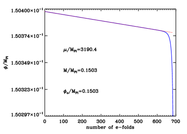
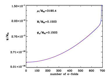
We now proceed with phase $1$. By definition, the second term on the right-hand side of the waterfall equation (3) can be neglected. This means that this equation, as was already the case for the inflaton equation of motion (which remains unaffected during phase $1$), becomes linear. For this reason, sometimes, this phase is also called the “linear phase.” During this phase, the solution for the inflaton field is unchanged but, of course, one now has to solve the new approximated equation for the waterfall field . The solution can be easily calculated and reads

$$\ln\frac{\psi}{\psi_{1}} = \frac{\mu^{2}}{M^{2}}\left[{\rm e}^{-4M_{\scriptscriptstyle{\mathrm{Pl}}}^{2}(N-N_{\mathrm{c}})/\mu^{2}}-{\rm e}^{-4M_{\scriptscriptstyle{\mathrm{Pl}}}^{2}(N_{1}-N_{\mathrm{c}})/\mu^{2}}\right]$$ (37)

$$+\frac{4M_{\scriptscriptstyle{\mathrm{Pl}}}^{2}}{M^{2}}\left(N-N_{1}\right).$$

Then, one can Taylor expand the exponential functions since we are in the regime where $\mu/M_{\scriptscriptstyle{\mathrm{Pl}}}\gg 1$. This gives

$$\psi=\psi_{1}\exp\left\{\frac{8M_{\scriptscriptstyle{\mathrm{Pl}}}^{4}}{\mu^{2}M^{2}}\left[\left(N-N_{\mathrm{c}}\right)^{2}-\left(N_{1}-N_{\mathrm{c}}\right)^{2}\right]\right\}.$$ (38)

This solution together with the solution for the inflaton is represented in Fig. 4. This plot confirms that the previous approximated solutions match the exact ones with a very good precision. Finally, in field space, the trajectory now reads

$$\psi=\psi_{1}\exp\left[\frac{2\mu^{2}}{M^{2}}\left(\ln^{2}\frac{\phi}{\phi_{\mathrm{c}}}-\ln^{2}\frac{\phi_{1}}{\phi_{\mathrm{c}}}\right)\right].$$ (39)

or, equivalently,

$$\ln^{2}\frac{\phi}{\phi_{\mathrm{c}}}=\ln^{2}\frac{\phi_{1}}{\phi_{\mathrm{c}}}+\frac{M^{2}}{2\mu^{2}}\ln\frac{\psi}{\psi_{1}}.$$ (40)

Phase $1$ stops when, on the right-hand side of the slow-roll inflaton equation of motion (2) for $\phi$, the last term becomes $1$. This occurs for $\psi\equiv\psi_{2}$, where

$$\psi_{2}^{2}=\frac{\phi_{\mathrm{c}}^{2}M^{2}}{2\mu^{2}}\,,$$ (41)

and $\phi=\phi_{2}$ with

$$\ln^{2}\frac{\phi_{2}}{\phi_{\mathrm{c}}} \simeq \ln^{2}\frac{\phi_{1}}{\phi_{\mathrm{c}}}+\frac{M^{2}}{2\mu^{2}}\ln\left(\frac{\phi_{\mathrm{c}}M}{\sqrt{2}\mu\psi_{1}}\right)$$ (42)

$$\simeq \frac{M^{2}}{2\mu^{2}}\ln\left(\frac{\phi_{\mathrm{c}}M}{\sqrt{2}\mu\psi_{\mathrm{c}}}\right)\,,$$ (43)

the last approximated relation being obtained under the assumption that phase $0$ can be neglected and, as a consequence, that $\phi_{1}\simeq\phi_{\mathrm{c}}$ and $\psi_{1}\simeq\psi_{\mathrm{c}}$. It is also important to realize that the terms $1-\phi^{2}/\phi_{\mathrm{c}}^{2}$ and $\psi^{2}/M^{2}$ are equal at the onset of phase $1$ and then both increase. It is therefore necessary to check that, at the end of phase $1$, the term $1-\phi^{2}/\phi_{\mathrm{c}}^{2}$ still dominates over $\psi^{2}/M^{2}$. In other words, one has to verify that $\psi^{2}/M^{2}$ has increased less rapidly than $1-\phi^{2}/\phi_{\mathrm{c}}^{2}$. Using the solution for the waterfall, one has

$$N_{2}-N_{\mathrm{c}}\simeq\frac{\mu M}{2\sqrt{2}M_{\scriptscriptstyle{\mathrm{Pl}}}^{2}}\ln^{1/2}\left(\frac{\psi_{2}}{\psi_{\mathrm{c}}}\right),$$ (44)

where $N_{2}$ denotes the number of e-folds at the end of phase $1$ or, equivalently, at onset of the phase $2$. Upon using this formula, this leads to

$$\frac{\phi_{2}^{2}}{\phi_{\mathrm{c}}^{2}}-1=-\sqrt{2}\frac{M}{\mu}\ln^{1/2}\left(\frac{\phi_{\mathrm{c}}M}{\sqrt{2}\mu\psi_{\mathrm{c}}}\right)\,,$$ (45)

an expression that should be compared with

$$\frac{\psi_{2}^{2}}{M^{2}}=\frac{\phi_{\mathrm{c}}^{2}}{2\mu^{2}}.$$ (46)

We see that the condition $\phi_{2}^{2}/\phi_{\mathrm{c}}^{2}-1\gg\psi_{2}^{2}/M^{2}$ is a priori not obvious. However, in the case under scrutiny in this article, one chooses $\phi_{\mathrm{c}}$ and $M$ to be roughly of the same order of magnitude and $\mu\gg M_{\scriptscriptstyle{\mathrm{Pl}}}$. As a consequence, the condition is satisfied since $\phi_{2}^{2}/\phi_{\mathrm{c}}^{2}-1$ scales as the inverse of $\mu$ (neglecting the influence of the logarithm) while $\psi_{2}^{2}/M^{2}$ scales as the inverse of $\mu^{2}$. However, it is also clear that one could easily design a situation where this is not true. Here, we restrict ourselves to situations where this does not happen.

Finally, let us express the number of e-folds produced during phase $1$. It is given by

$$N_{2}-N_{\mathrm{c}}\simeq\frac{\mu M}{2\sqrt{2}M_{\scriptscriptstyle{\mathrm{Pl}}}^{2}}\ln^{1/2}\left(\frac{\phi_{\mathrm{c}}M}{\sqrt{2}\mu\psi_{\mathrm{c}}}\right).$$ (47)

Upon using Eq. (25), one could also replace $\psi_{\mathrm{c}}$ by its expression in the above equation to obtain a formula depending on the initial conditions. We see that the number of e-folds during phase $1$ is essentially controlled by the ratio $\mu M/M_{\scriptscriptstyle{\mathrm{Pl}}}^{2}$. This conclusion is in agreement with the results of Ref. Kodama et al. (2011). As a consequence, for $\mu M/M_{\scriptscriptstyle{\mathrm{Pl}}}^{2}>1$, $N_{2}-N_{\mathrm{c}}$ can be large. Hence, we conclude that the number of e-folds during the waterfall phase can indeed be much greater than the $60$ required for inflation to be successful as was noticed in Ref. Clesse (2011). The previous considerations allow us to identify where, in the parameter space, this regime occurs. We have studied this classical phase of evolution in some detail because this regime is of particular interest for the present article. Indeed, in the next section, we show that in this case the quantum effects play an important role.

Figure 5: Classical background evolution of the inflaton and waterfall fields starting from the critical point, $\phi=\phi_{\mathrm{c}}$ and $\psi=10^{-12}M_{\scriptscriptstyle{\mathrm{Pl}}}$. The solid blue curve represents the exact (i.e. numerical) trajectory while the dotted red curve is the slow-roll approximation during phase $1$ and the dotted green curve is the slow-roll approximation during phase $2$. The inset shows the overall evolution of the two fields with, in particular, the oscillations around the true minimum of the potential at the end of inflation.

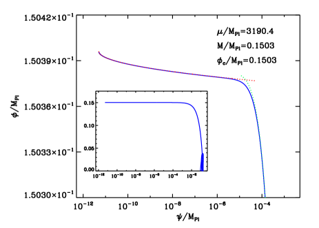
Let us now briefly mention phase $2$ (it was studied in more detail in Ref. Kodama et al. (2011)). This time one needs to keep the last term in the inflaton equation of motion (2). This means that the evolution for $\phi$ is modified and, as a consequence, the formula giving $\psi(N)$ is no longer valid since it made use of the evolution for $\phi$ established before. In this regime the Eq. (2) and (3) become fully coupled. However, it is still possible to find the slow-roll trajectory in the field space. One obtains Kodama et al. (2011)

$$\frac{{\rm d}\phi}{{\rm d}\psi}=\frac{\phi\psi}{\phi^{2}-\phi^{2}_{\mathrm{c}}}\,$$ (48)

which can be easily integrated, and the solution reads

$$\psi^{2}=\psi_{2}^{2}+\phi^{2}-\phi_{2}^{2}-2\phi_{\mathrm{c}}^{2}\ln\frac{\phi}{\phi_{2}}.$$ (49)

This expression (green dotted line) is compared to the exact numerical solution (blue solid line) in Fig. 5. Clearly, the agreement is excellent. During phase $2$, inflation stops and the system starts oscillating around one of the two true minimums of the potential. This is the onset of the reheating phase.

The above considerations complete this section. Having mastered the classical dynamics of the fields in the valley and during the waterfall regime, we are now in a position where we can turn to the main topic of this article, namely, studying the role played by the quantum effects. This is the goal of the next section.

III Stochastic Effects

In this article, we use the stochastic inflation formalism to study the quantum effects. In this formalism, an effective Langevin equation can be derived for the “coarse-grained” field, i.e. the original field averaged over a physical volume the size of which is typically larger than the Hubble radius $H^{-1}$. Applied to the case of hybrid inflation, one obtains two coupled Langevin equations for the inflaton and the waterfall fields, respectively. They read

$$3H^{2}\frac{\mathrm{d}\phi}{\mathrm{d}N} = -\frac{2\Lambda^{4}\phi}{\mu^{2}}\left(1+\frac{2\psi^{2}\mu^{2}}{\phi_{\mathrm{c}}^{2}M^{2}}\right)+\frac{3H^{3}}{2\pi}\xi_{\phi}\left(N\right)\,,$$ (50)

$$3H^{2}\frac{\mathrm{d}\psi}{\mathrm{d}N} = -\frac{4\Lambda^{4}}{M^{2}}\psi\left(\frac{\phi^{2}-\phi_{\mathrm{c}}^{2}}{\phi_{\mathrm{c}}^{2}}+\frac{\psi^{2}}{M^{2}}\right)+\frac{3H^{3}}{2\pi}\xi_{\psi}\left(N\right)\,,$$

where $\xi_{\phi}$ and $\xi_{\psi}$ are two uncorrelated white Gaussian noises with $0$-mean and $1$-variance. Notice that the time variable used is the number of e-folds. It was argued in Refs. Finelli et al. (2009, 2010, 2011) that this choice is preferred.

III.1 Can the Quantum Effects Be Important?

Having at our disposal the two Langevin equations presented above, the first question is whether the stochastic noises can really play an important role and, if so, where in the field plane. This issue can be addressed in the following manner. During a typical time interval $\Delta t=H^{-1}$, both stochastic and classical evolutions of the fields $\phi$ and $\psi$ can be read off directly from Eqs. (50) and (III). Roughly speaking, the typical classical change in the inflaton value is $\simeq M_{\scriptscriptstyle{\mathrm{Pl}}}^{2}(\partial V/\partial\phi)/V$, while the magnitude of the quantum kick is $H/(2\pi)$. Therefore, in order to assess the relative contribution of the stochastic effects over the classical ones, one can study the ratios $\Delta_{\phi}$ and $\Delta_{\psi}$ of these two quantities for each field (in the context of a quartic large field model, this is how one can deduce that the quantum corrections dominate if the value of the field is larger than $\lambda^{-1/6}M_{\scriptscriptstyle{\mathrm{Pl}}}$, where $\lambda$ is the self-coupling constant that appears in the potential). This amounts to taking $\Delta_{\phi}\equiv V^{3/2}/[2\pi\sqrt{3}M_{\scriptscriptstyle{\mathrm{Pl}}}^{3}(\partial V/\partial\phi)]$ and a similar definition for $\Delta_{\psi}$. In the vacuum dominated regime, the two quantities $\Delta_{\phi}$ and $\Delta_{\psi}$ read

$$\Delta_{\phi} = \frac{1}{4\pi\sqrt{3}}\frac{\Lambda^{2}\phi_{\mathrm{c}}}{M_{\scriptscriptstyle{\mathrm{Pl}}}^{3}}\frac{\phi_{\mathrm{c}}}{\phi}\left(\frac{\phi_{\mathrm{c}}^{2}}{\mu^{2}}+2\frac{\psi^{2}}{M^{2}}\right)^{-1}\,,$$ (52)

$$\Delta_{\psi} = \frac{1}{8\pi\sqrt{3}}\frac{\Lambda^{2}M}{M_{\scriptscriptstyle{\mathrm{Pl}}}^{3}}\frac{M}{\psi}\left(\frac{\psi^{2}}{M^{2}}-1+\frac{\phi^{2}}{\phi_{\mathrm{c}}^{2}}\right)^{-1}\,.$$ (53)

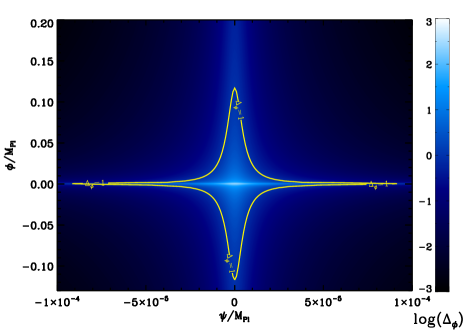
These quantities are plotted in Fig. 6 in the $(\phi,\psi)$ plane. Values such that $\Delta>1$ indicate that the quantum effects dominate.

Figure 6: $\Delta_{\phi}$ and $\Delta_{\psi}$ plotted in the $\left(\phi,\psi\right)$ plane for the parameters $\mu=3190.4\,M_{\scriptscriptstyle{\mathrm{Pl}}}$, $M=\phi_{\mathrm{c}}=0.1503\,M_{\scriptscriptstyle{\mathrm{Pl}}}$, $\Lambda=0.01418\,M_{\scriptscriptstyle{\mathrm{Pl}}}$. $\Delta_{\phi}$ and/or $\Delta_{\psi}$ greater than $1$ ($\sim$ in white on the plot) signal that the quantum effects are dominant. The stochastic effects in the $\psi$ direction obviously dominate over the classical contributions in the valley and around the critical point, while the stochastic effects in the $\phi$ direction dominate in the valley and around the origin.

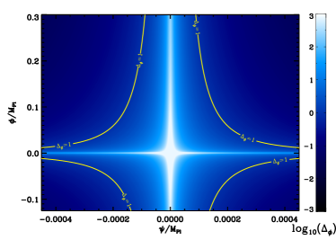
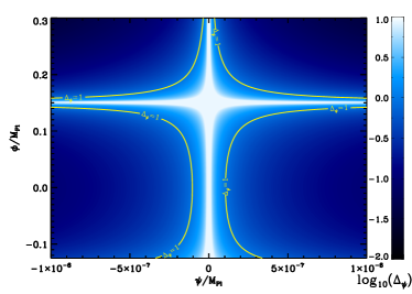
Let us now discuss how $\Delta_{\phi}$ and $\Delta_{\psi}$ behave in the field plane. Clearly, $\Delta_{\phi}$ is infinite when $\phi=0$ for any values of $\psi$. Therefore, the quantum effects are dominant along that direction. In the inflationary valley $\psi=0$, which is perpendicular to the previously mentioned direction, one has

$$\Delta_{\phi}^{\rm valley}=\frac{1}{4\pi\sqrt{3}}\frac{\Lambda^{2}\mu^{2}}{M_{\scriptscriptstyle{\mathrm{Pl}}}^{3}\phi}.$$ (54)

This means that $\Delta_{\phi}>1$ as long as

$$\frac{\phi}{M_{\scriptscriptstyle{\mathrm{Pl}}}}<\frac{\phi^{\rm valley}}{M_{\scriptscriptstyle{\mathrm{Pl}}}}\equiv\frac{1}{4\pi\sqrt{3}}\frac{\Lambda^{2}\mu^{2}}{M_{\scriptscriptstyle{\mathrm{Pl}}}^{4}}.$$ (55)

For the parameters used in Fig. 6, one has $\phi^{\rm valley}/M_{\scriptscriptstyle{\mathrm{Pl}}}\simeq 94$, i.e. a value much larger than the upper limit of this plot. This means that the quantum effects dominate “very high” in the valley and, in particular, around the critical point. The previous considerations explain the cross-shaped white region centered at the origin observed in Fig. 6. In this regime, one expects a faithful description of the system to be obtained only if the stochastic noises for the two coupled fields are taken into account. In the following, we study this case, where treating one field (for instance, the inflaton) classically and the other (the waterfall field) stochastically is a priori not a good approximation.

Of course, these results also depend on the parameters, in particular, on $\Lambda$. It is interesting to determine the value of $\Lambda\equiv\Lambda_{\phi}$ such that $\phi^{\rm valley}=\phi_{\mathrm{c}}$. This value indicates the limit between the regime where it is mandatory to take into account the noise both in the inflaton and waterfall field directions and the regime where the waterfall field is still stochastic but where it is sufficient to treat the inflaton classically. It is given by

$$\Lambda_{\phi}^{2}=4\pi\sqrt{3}\frac{\phi_{\mathrm{c}}M_{\scriptscriptstyle{\mathrm{Pl}}}^{3}}{\mu^{2}}$$ (56)

For our fiducial parameters, this leads to $\Lambda_{\phi}\simeq 5.7\times 10^{-4}M_{\scriptscriptstyle{\mathrm{Pl}}}$. Obviously, for larger values of $\mu$, $\Lambda_{\phi}$ is even smaller. In Fig. 7, we have represented $\Delta_{\phi}$ for the same parameters, except that $\Lambda=5\times 10^{-4}M_{\scriptscriptstyle{\mathrm{Pl}}}\lesssim\Lambda_{\phi}$. This plot confirms that the region $\Delta_{\phi}>1$ covers a much smaller area which does not encompass the critical point. In that case $\phi$ should behave almost classically in the valley, and we will also investigate this regime in Sec. III.4.

Let us now describe $\Delta_{\psi}$. It is infinite for $\psi=0$, that is to say, in the valley. When $\psi\neq 0$, the quantum effects are dominant when $\phi^{2}/\phi_{\mathrm{c}}^{2}\simeq 1-\psi^{2}/M^{2}$, i.e. in the direction $\phi\simeq\phi_{\mathrm{c}}$ perpendicular to the valley (in the regime where $\psi/M\ll 1$). This explains the cross-shaped white region, this time centered at the critical point; see Fig. 6. This time, the previous considerations do not depend on $\Lambda$, which means that the noise in the waterfall field should always be taken into account in the valley and around the critical point. Since this corresponds to a very flat region of the potential where most of the e-folds are realized, one can already expect the inflationary dynamics to be significantly affected by the quantum effects.

Figure 7: $\Delta_{\phi}$ plotted in the $\left(\phi,\psi\right)$ plane for the parameters $\mu=3190.4\,M_{\scriptscriptstyle{\mathrm{Pl}}}$, $M=\phi_{\mathrm{c}}=0.1503\,M_{\scriptscriptstyle{\mathrm{Pl}}}$, $\Lambda=0.0005M_{\scriptscriptstyle{\mathrm{Pl}}}\lesssim\Lambda_{\phi}$. For this value of $\Lambda$, $\Delta_{\phi}$ remains small along the valley and does not encompass the critical point. It becomes larger than $1$ only in the vicinity of the origin.

III.2 Obstacles to a Perturbative Approach

Having justified that the quantum corrections play a crucial role, the next question is how to compute them, i.e. how to solve the two Langevin equations. It is clear that an exact analytical solution is not available. However, as proposed in Refs. Martin and Musso (2006a, b), the Langevin equation can be solved perturbatively by considering the coarse-grained field as a perturbation on top of the classical solution. The corresponding formalism in the case of single field inflation was presented in Ref. Martin and Musso (2006a). However, in the present case, we are in a two-field situation, which means that both the inflaton and the waterfall fields must be expanded according to

$$\phi\left(N\right) = \phi_{\mathrm{cl}}\left(N\right)+\delta\phi_{1}\left(N\right)+\delta\phi_{2}\left(N\right)+...,$$ (57)

$$\psi\left(N\right) = \psi_{\mathrm{cl}}\left(N\right)+\delta\psi_{1}\left(N\right)+\delta\psi_{2}\left(N\right)+...,$$ (58)

where $\phi_{\mathrm{cl}}$ and $\psi_{\mathrm{cl}}$ are the classical values. We see that the corrections to the classical solutions are obtained by adding successive terms of higher and higher powers in the noise. In Ref. Martin and Musso (2006a), general formulas, valid at second order, are provided, leading to a Gaussian probability density function for the field. The validity of this approach relies on the smallness of the stochastic effects compared to the classical ones and, obviously, the expansion is valid only in a limited regime; see Ref. Martin and Musso (2006b). Here, we have just seen that the quantum effects are dominant around the critical point and, therefore, there are already reasons to guess that a perturbative approach is not very appropriate.

Moreover, one can see that the perturbative approach is technically impossible to carry out in a multiple field situation since even the linearized coupled stochastic differential equations cannot be analytically solved. Indeed, in the hybrid inflation case, at first order in the noise, they can be written as

$$\frac{\mathrm{d}\delta\phi_{1}}{\mathrm{d}N}+2\delta\psi_{1}\left(\frac{H_{\phi\psi}}{H}-\frac{H_{\psi}H_{\phi}}{H^{2}}\right)$$

$$+2\delta\phi_{1}\left(\frac{H_{\phi\phi}}{H}-\frac{H_{\phi}^{2}}{H^{2}}\right)=\frac{H}{2\pi}\xi_{\phi}\left(N\right),$$ (59)

$$\frac{\mathrm{d}\delta\psi_{1}}{\mathrm{d}N}+2\delta\phi_{1}\left(\frac{H_{\phi\psi}}{H}-\frac{H_{\psi}H_{\phi}}{H^{2}}\right)$$

$$+2\delta\psi_{1}\left(\frac{H_{\psi\psi}}{H}-\frac{H_{\psi}^{2}}{H^{2}}\right)=\frac{H}{2\pi}\xi_{\psi}\left(N\right)\,,$$ (60)

where $H_{\phi}$ is the derivative of $H=\sqrt{V}/\left(M_{\scriptscriptstyle{\mathrm{Pl}}}\sqrt{3}\right)$ with respect to $\phi$ and the other notations used in this equation straightforwardly follow. The matrix of this differential system does not commute with itself at different times $N$ and, as a consequence, one cannot solve the coupled perturbative problem in a simple way.

III.3 Testing the Numerical Approach

Figure 8: Numerical predictions for $\langle\psi_{\mathrm{c}}^{2}\rangle_{\mathrm{num}}$ normalized to $\langle\psi_{\mathrm{c}}^{2}\rangle_{\mathrm{pert}}$ given by Eq. (61) for different values of $\Lambda$ normalized to $\Lambda_{\phi}$ defined in Eq. (56).

For all these reasons, the only method left seems to be a full numerical integration of the stochastic inflationary equations. This is the method used in the present article. Since the differential equations to be solved turn out to be stiff most of the time, we use a fourth order Rosenbrock method, monitoring a local truncation error to adjust step sizes, that we have adapted to take into account the presence of an extra random stochastic term. When possible, we have also used the Euler-Muruyama method in another independent code in order to check our numerical results.

Figure 9: Stochastic trajectories in field space for different values of $\Lambda$: $\Lambda=\Lambda_{\phi}/20$ (top left panel), $\Lambda=\Lambda_{\phi}/10$ (top right panel), $\Lambda=\Lambda_{\phi}$ (bottom left panel), and $\Lambda=10\Lambda_{\phi}$ (bottom right panel). The solid black line represents the classical trajectory starting from the point $\phi_{\mathrm{in}}=1.0001\phi_{\mathrm{c}}$ and $\psi_{\mathrm{in}}=6.6\times 10^{-5}M$. The blue, cyan, pink, and purple lines represent four different stochastic trajectories. The parameters chosen are $\mu/M_{\scriptscriptstyle{\mathrm{Pl}}}=3190.4$ and $M/M_{\scriptscriptstyle{\mathrm{Pl}}}=\phi_{\mathrm{c}}/M_{\scriptscriptstyle{\mathrm{Pl}}}\simeq 0.1503$. The contours $\Delta_{\phi}=1$ (solid red line) and $\Delta_{\psi}=1$ (solid green line) are also represented.

In this section, we describe the tests that we have performed in order to check that our numerical codes work properly. A first verification of the consistency of our numerical treatment can be obtained in the following manner. If one considers that the dynamics of $\phi$ remains classical in the valley, then following Refs. Garcia-Bellido et al. (1996); Clesse (2011) one can perturbatively estimate the typical dispersion of the waterfall field distribution (i.e. in the $\psi$ direction) at the critical point. One obtains

$$\langle\psi_{\mathrm{c}}^{2}\rangle_{\mathrm{pert}}\simeq\frac{H^{2}\mu M}{32\pi^{3/2}M_{\scriptscriptstyle{\mathrm{Pl}}}^{2}}\,.$$ (61)

Therefore, numerically, in the regime $\Lambda<\Lambda_{\phi}$ (to ensure that the inflaton field behaves classically), one should recover the same result. As a consequence, it is interesting to plot the quantity $(\langle\psi_{\mathrm{c}}^{2}\rangle_{\mathrm{num}}/\langle\psi_{\mathrm{c}}^{2}\rangle_{\mathrm{pert}})^{1/2}$, where $\langle\psi_{\mathrm{c}}^{2}\rangle_{\mathrm{num}}$ is the dispersion in the waterfall direction (at $\phi=\phi_{\mathrm{c}}$) obtained numerically. This quantity as a function of $\Lambda/\Lambda_{\phi}$ is represented in Fig. 8. As it is clear from this plot, when $\Lambda<\Lambda_{\phi}$, the ratio $(\langle\psi_{\mathrm{c}}^{2}\rangle_{\mathrm{num}}/\langle\psi_{\mathrm{c}}^{2}\rangle_{\mathrm{pert}})^{1/2}$ is precisely $1$, thus showing that our code correctly reproduces the known analytical result. We also see that when $\Lambda>\Lambda_{\phi}$, the perturbative regime breaks down. From what we have just discussed, the interpretation of this result is clearly that the stochastic effects in the $\phi$ direction play a role and kick the system below the critical point more rapidly. As a consequence, the distribution in $\psi$ has much less e-folds to broaden than classically predicted, and hence $\langle\psi_{\mathrm{c}}^{2}\rangle_{\mathrm{num}}<\langle\psi_{\mathrm{c}}^{2}\rangle_{\mathrm{pert}}$. This behavior is similar to what has been found in Ref. Enqvist et al. (2011), where it has been shown that, in case of a multiple field inflationary dynamics with one flat direction and several nonflat directions, the fluctuations of the nonflat directions can be sufficient to block the growth of the root-mean-square amplitude along the flat direction. The fact that $\langle\psi_{\mathrm{c}}^{2}\rangle_{\mathrm{num}}$ deviates from $\langle\psi_{\mathrm{c}}^{2}\rangle_{\mathrm{pert}}$ precisely at $\Lambda=\Lambda_{\phi}$ is another indication of the consistency of our numerical results.

Figure 10: Probability density functions in the $\left(\phi,\psi\right)$ plane, at different times $N$, starting from a Dirac distribution in the valley. The parameters chosen are $\Lambda=1.06347\,M_{\scriptscriptstyle{\mathrm{Pl}}}$, $\phi_{\mathrm{c}}=M=1.50398\,M_{\scriptscriptstyle{\mathrm{Pl}}}$, and $\mu=7.74597\,M_{\scriptscriptstyle{\mathrm{Pl}}}$.

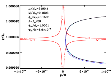
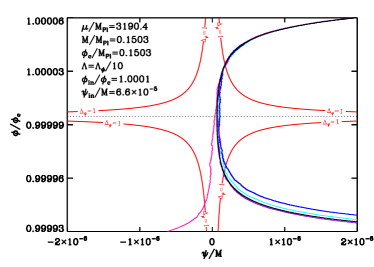
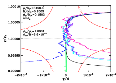
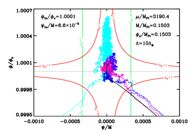
Another type of consistency check can also be performed by investigating how given realizations behave for different values of the parameters. We present in Fig. 9 four different examples, for four different values of $\Lambda$, where four stochastic realizations (blue, cyan, purple, and pink lines) are compared with the classical trajectory (solid black line). The top left panel corresponds to $\Lambda=\Lambda_{\phi}/20$. In this case, the noise is so small that the four stochastic realizations almost follow the classical trajectory. The top right panel corresponds to $\Lambda=\Lambda_{\phi}/10$, and the noise in the inflaton direction still plays no role in this case (i.e. the contour $\Delta_{\phi}=1$ does not encompass the critical point). One sees that, when the trajectories enter the $\Delta_{\psi}>1$ region, they start feeling the noise and that one of them (the pink realization) is even expelled towards the other global minimum. The bottom left panel corresponds to $\Lambda=\Lambda_{\phi}$, and the noise is stronger as revealed by the “shaky” behavior of the realizations. The contour $\Delta_{\phi}=1$ appears but, clearly, the noise in the waterfall direction remains the main source of stochasticity. Finally, the bottom right panel corresponds to $\Lambda=10\Lambda_{\phi}$ and, this time, we are in a regime where the noise in the two directions is a priori important as indicated by the contours $\Delta_{\phi}=1$ and $\Delta_{\psi}=1$. This is especially clear for the cyan realization which climbs the inflationary valley. Therefore, it seems fair to say that our numerical code gives results that are completely compatible with elementary expectations, which is an indication that it correctly calculates the behavior of the system.

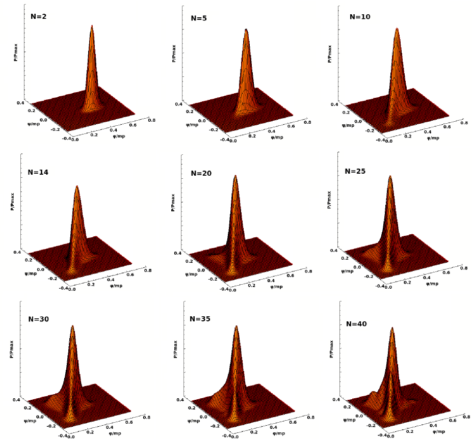
Finally, by simulating a high number of realizations, we have been able to calculate the correlation functions of various quantities of interest as well as their probability distributions. As an example, Fig. 10 shows the probability density function in the $\left(\phi,\psi\right)$ plane, at different times $N$, starting from a peaked distribution in the valley. One can see that the distribution is first roughly Gaussian and goes down the valley before setting over the critical point with “excrescences” growing towards the two minimums of the potential, rendering the distribution highly non-Gaussian. Again, this plot confirms the previous discussion and shows that the numerical codes used in this article are able to reproduce expected results in regimes where it is possible to guess (or to approximately calculate) the behavior of the system.

In the following subsections, we present in more detail our numerical results.

III.4 Number of e-folds

Figure 11: Distribution of the total number of e-folds realized during inflation. Classically, $505$ e-folds are realized in the valley and $747$ e-folds are realized during the waterfall stage, accounting for a total of $1252$ e-folds. Clearly the mean value $\langle N\rangle\sim 50$ is very different from the classical value which illustrates well how important the stochastic effects in the vicinity of the critical point are. Despite this fact, it is also interesting to notice that, in the tail of the distribution, one can find realizations with a total number of e-folds larger than the classical value.

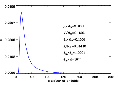
A first relevant well-defined physical quantity to study is the total number of e-folds realized during inflation since it provides a straightforward way to investigate the deviations from the classical picture. Of course, in order to calculate this quantity, one has to choose some initial conditions. Here, we take $\phi_{\mathrm{in}}/\phi_{\mathrm{c}}=1.0001$ and $\psi_{\mathrm{in}}/M=10^{-9}$. The parameters describing the shape of the potential are $\mu/M_{\scriptscriptstyle{\mathrm{Pl}}}=3190.4$, $M=\phi_{\mathrm{c}}=0.1503M_{\scriptscriptstyle{\mathrm{Pl}}}$, and $\Lambda/M_{\scriptscriptstyle{\mathrm{Pl}}}=0.01418$. We see that this implies $\mu M/M_{\scriptscriptstyle{\mathrm{Pl}}}^{2}>1$ and, therefore, we already know from the previous section that the number of e-folds during the waterfall phase will be large. As a matter of fact, it can be easily estimated upon using Eq. (47). The above described choice is made in order to illustrate our point in the clearest way. It is important to stress that choosing other initial conditions would not drastically modify our conclusions. The classical prediction can be calculated in the slow-roll approximation using the formulas derived above, or using a numerical integration of the exact equations. It leads to a trajectory such that $\sim 505$ e-folds are realized in the valley and $\sim 747$ during the waterfall regime. The total number of e-folds is therefore $\sim 1252$.

Figure 12: Distribution of the total number of e-folds realized during inflation, normalized by its maximum value, for different values of $\mu$. The dependence on $\mu$ of $\langle N\rangle$ is consistent with the qualitative predictions of Sec. II. One also notices that the dispersion of the distribution increases with the number of e-folds realized in the flat region. This is due to the fact that the quantum effects broaden the distribution.

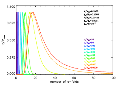
Then, we have computed the same quantity (for the same values of the initial conditions and of the parameters) in the stochastic case. Obviously, for each realization one gets a different number, and the corresponding distribution is displayed in Fig. 11. Let us now discuss this figure. Probably, the most striking property of Fig. 11 is that the distribution is peaked at a value which is completely different from the classical prediction. This clearly means that strong non-perturbative effects are at play. This also emphasizes the necessity of using a full numerical approach. Moreover, one sees that the stochastic contribution tends to diminish the total number of e-folds. This fact can be intuitively understood by noticing that most e-folds are realized in the region where the potential is very flat, around the critical point. Since this is precisely where the stochastic terms are dominant, the quantum kicks remove the system away from this region much faster than the classical roll; hence a lower number of e-folds is realized in this region.

The tendency to escape faster from a region where the potential is very flat can be understood analytically on the example of small field inflation. In this single field model, the potential is given by

$$V\left(\psi\right)=M^{4}\left[1-\left(\frac{\psi}{\mu}\right)^{p}\right]\,,$$ (62)

where $\mu$ is a mass scale. Inflation proceeds from small to large values of the field. At the beginning of inflation, the potential is very flat and a large number of e-folds can be realized. For $p=2$, the slow-roll and the perturbative Langevin equations can be integrated and solved exactly; see Ref. Martin and Musso (2006a). Following Ref. Gratton and Turok (2005), one can then calculate the mean value of the total number of e-folds,

$$\langle N\rangle=-\frac{1}{2M_{\scriptscriptstyle{\mathrm{Pl}}}^{2}}\int_{\psi_{\mathrm{in}}}^{\psi}{\rm d}\psi\frac{\langle H\rangle}{H^{\prime}_{\mathrm{cl}}}\,.$$ (63)

In the present case and since $\phi\ll\mu$, one obtains

$$\langle N\rangle \simeq N_{\mathrm{class}}-\frac{1}{192\pi^{2}}\left(\frac{M}{M_{\scriptscriptstyle{\mathrm{Pl}}}}\right)^{4}\left(\frac{\mu}{M_{\scriptscriptstyle{\mathrm{Pl}}}}\right)^{2}$$ (64)

$$\times \left[\ln\left(\frac{\psi_{\mathrm{in}}}{\psi}\right)+\frac{1}{2}\left(\frac{\psi^{2}}{\psi_{\mathrm{in}}^{2}}-1\right)\right],$$

where $N_{\mathrm{class}}$ is the number of e-folds classically realized. From the above expression, it is clear that $\langle N\rangle$ is smaller than $N_{\mathrm{class}}$ since $\psi_{\mathrm{in}}<\psi_{\mathrm{end}}$ in this model. This result confirms the previous considerations: when the potential is very flat, the quantum kicks undergone by the inflaton field push it out of the flat region and, as a consequence, the total number of e-folds becomes smaller.

Figure 13: Total number of e-folds (blue) and number of e-folds realized in the valley (green) as a function of $\Lambda/M_{\scriptscriptstyle{\mathrm{Pl}}}$ for the parameters indicated on the plot. The two numbers of e-folds are normalized to their classical counterparts. The solid lines represent the mean values of the distributions, while the colored surfaces represent the plus or minus $1$ standard deviation areas. The vertical solid black line indicates the value of $\Lambda_{\phi}$.

Finally, it is also interesting to study how our results depend on the parameters of the model, especially on $\mu$ and $\Lambda$. As an example, Fig. 12 shows the normalized distribution of the total number of e-folds for different values of the parameter $\mu$. From Eqs. (16) and (47), one can see that the classical number of e-folds realized during both the inflationary valley and the waterfall regime increases with $\mu$, which is consistent with the behavior of the mean values of the stochastic distributions observed in Fig. 12. Moreover, the longer the field system stays in the flat region close to the critical point, the more its distribution gets stochastically broadened. This means that the dispersion of the distribution should evolve in a similar manner, which is exactly what is seen in Fig. 12. Moreover, if one keeps increasing $\mu$, one observes that the mean value of the distribution saturates at a value of $\simeq 60$ e-folds.

Figure 14: Number of e-folds realized between the exit of the stochastic regime (i.e. the moment where $\Delta_{\phi}$ and $\Delta_{\psi}$ are both smaller than $1$) and the end of inflation. The cruxes stand for the mean values of the distributions, and the colored surfaces stand for the plus or minus $1$ standard deviation areas. The horizontal dotted red line represents the total number of e-folds calculated in the absence of noise. The horizontal dotted orange line is the number of e-folds realized in the waterfall region in the absence of noise. Finally, the horizontal green dotted line represents the minimal number of e-folds required for inflation to be successful, i.e. $60$.

As mentioned above, we have also studied how our results depend on $\Lambda$. In the vacuum dominated regime, $\Lambda$ is directly related to the energy scale of inflation. This quantity is constrained by the big bang nucleosynthesis and by the observations of the CMBR, namely,

$$10^{-17}M_{\scriptscriptstyle{\mathrm{Pl}}}\lesssim\Lambda\lesssim 5\times 10^{-2}M_{\scriptscriptstyle{\mathrm{Pl}}}\,.$$ (65)

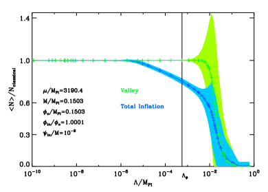
The previous figures correspond to a regime where $\Lambda>\Lambda_{\phi}$ (recall that, for the values of the parameters chosen here, we have $\Lambda_{\phi}\simeq 5.7\times 10^{-4}M_{\scriptscriptstyle{\mathrm{Pl}}}$) since we wanted to study a regime where the noise in the two-field directions is important. However, one can also wonder if the previous conclusions, especially the fact that $\langle N\rangle<N_{\rm class}$, still hold in the regime $\Lambda<\Lambda_{\phi}$. In Fig. 13, we have computed the total number of e-folds as a function of $\Lambda$. The first thing we notice in this plot is that, for $\Lambda\gtrsim\Lambda_{\phi}$ (indicated by the vertical black line), the total number of e-folds and the number of e-folds in the valley are smaller than their classical counterparts. This is of course compatible with the previous considerations. In the regime $10^{-6}M_{\scriptscriptstyle{\mathrm{Pl}}}\lesssim\Lambda\lesssim\Lambda_{\phi}$, the number of e-folds in the valley is equal to its classical counterpart as expected since the inflaton behaves classically but the total number of e-folds, hence the number of e-folds in the waterfall regime, is still smaller than $N_{\rm class}$. So even in the absence of noise along the inflaton direction, the conclusion obtained before remains valid. Finally, for $\Lambda\lesssim 10^{-6}M_{\scriptscriptstyle{\mathrm{Pl}}}$, the noise is so small that the stochastic and classical number of e-folds are equal.

Figure 15: Level lines $\epsilon_{1}=1$ in the $\left(\phi,\psi\right)$ plane. The parameters chosen are the same as in the other plots. The red rhombus sits at the critical point, while the two green ones are located at the two minima. The definition of the angle $\theta$ is shown for a trajectory leaving the inflationary region (i.e. crossing the $\epsilon_{1}=1$ line) at the black square.

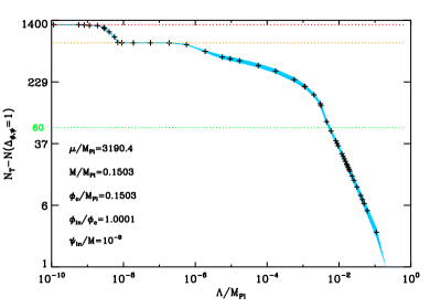
In Fig. 11, we have seen that, for $\Lambda=0.01418M_{\scriptscriptstyle{\mathrm{Pl}}}$, one has $\langle N\rangle\simeq 50$. Since the scales of astrophysical interest today left the Hubble radius during inflation about $50-60$ e-folds before the end of inflation, this would mean that we could have a direct observational window on the stochastic regime. In fact, this is not so because $\Delta=1$ means that $H^{2}/\epsilon_{1}\simeq 1$. But $H^{2}/\epsilon_{1}$ is precisely the overall normalization of the density perturbations power spectrum which is observed to be $\simeq 10^{-5}$. So, in fact, this shows that the value $\Lambda=0.01418M_{\scriptscriptstyle{\mathrm{Pl}}}$ is simply excluded by the CMBR measurements. For this reason, it is interesting to plot the number of e-folds performed between the moment the system becomes classical (i.e. when $\Delta_{\phi}$ and $\Delta_{\psi}$ are both smaller than $1$) and the end of inflation. If this number is smaller than $\sim 50-60$, this means that the corresponding value of $\Lambda$ is excluded due to the above argument. The plot is represented in Fig. 14. We see that for $\Lambda\gtrsim 10^{-2}M_{\scriptscriptstyle{\mathrm{Pl}}}$, the number mentioned above is indeed smaller than $60$. All these values are therefore excluded. This means that for values of $\Lambda$ such that $\Lambda_{\phi}\lesssim\Lambda\lesssim 10^{-2}M_{\scriptscriptstyle{\mathrm{Pl}}}$, we are in a regime where the perturbations are not too large to be directly in contradiction with the CMBR (of course this does not guarantee that the correct normalization can be obtained) and where it is mandatory to take into account the stochastic effects in the two-field directions. If $10^{-6}M_{\scriptscriptstyle{\mathrm{Pl}}}<\Lambda<\Lambda_{\phi}$, the stochastic effects dominate only in the $\psi$ direction, both in the valley and the waterfall phase. For $10^{-8}M_{\scriptscriptstyle{\mathrm{Pl}}}\lesssim\Lambda\lesssim 10^{-6}M_{\scriptscriptstyle{\mathrm{Pl}}}$, the waterfall regime becomes completely classical and, finally, for $\Lambda\lesssim 10^{-8}M_{\scriptscriptstyle{\mathrm{Pl}}}$, the noise becomes so small that the full evolution in the valley and in the waterfall region can be described classically.

Let us end this subsection with some remarks. We have seen that the stochastic number of e-folds is smaller than its classical counterpart as soon as $\Lambda\gtrsim 10^{-6}M_{\scriptscriptstyle{\mathrm{Pl}}}$. If $\Lambda\gtrsim\Lambda_{\phi}\simeq 5.7\times 10^{-4}M_{\scriptscriptstyle{\mathrm{Pl}}}$, we are in a two-field regime. Moreover, if $\Lambda\gtrsim 10^{-2}M_{\scriptscriptstyle{\mathrm{Pl}}}$, the stochastic effects are so strong that the model is in contradiction with the amplitude of the CMBR fluctuations. We expect these conclusions to be very roughly independent of the choice of the other parameters, provided, of course, that one remains in the regime described in Sec. II.1. In fact, to go further, one should explore the full parameter space, and one should carefully apply Cosmic Background Explorer (COBE) normalization to the model. When the waterfall regime plays an important role, this is not a trivial task.

III.5 Inflation Exit Point

Figure 16: Numerical distribution of the exit angle $\theta$. The parameters are the same as in the other figures. The red line corresponds to the classical prediction. We notice that the distribution is extremely peaked, $\Delta\theta/\theta\sim 10^{-3}$.

Figure 17: Flow map of the classical slow-roll dynamics equations. Regardless of their initial conditions, all the trajectories end up at the same exit point.

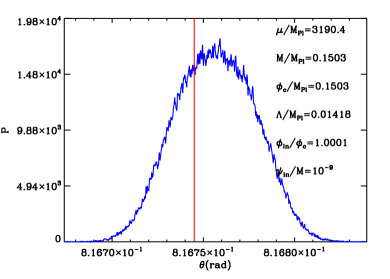
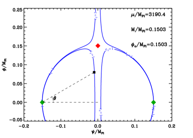
Another relevant physical quantity is the inflation exit point, i.e. the location in the field space where inflation stops. The details of the subsequent (p)reheating phase strongly depend on these initial conditions, which are therefore important physical quantities Garcia-Bellido and Linde (1998); Finelli and Brandenberger (2000). Inflation stops when the system crosses the $\epsilon_{1}=1$ level line in the field space. As a consequence, the exit point is necessarily located on this level line. It can be characterized by the angle $\theta$ between the line joining the closest minimum to the origin and the line joining this same minimum to the exit point. This parametrization and the $\epsilon_{1}=1$ contours are represented in Fig. 15. Since the stochastic effects taking place in the valley quickly render the distribution symmetrical in $\psi$, the two minima are in fact put on an equal footing. Using the same method as before, one can calculate the classical prediction for this angle $\theta$ and compare it with the corresponding stochastic distribution. The result is shown in Fig. 16.

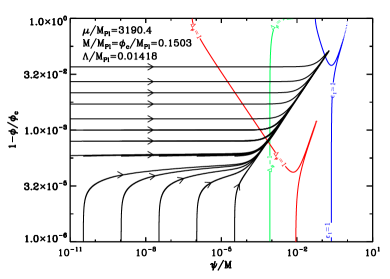
Here again, several comments are in order. First, unlike the distribution of the number of e-folds, the classical prediction lies within the stochastic distribution. It is even more remarkable that the distribution is very narrow. A priori, this is a surprising fact since the stochastic realizations in the vicinity of the critical point are extremely noisy, as can be seen in Fig. 9. Even if the stochastic trajectories are very different from one realization to another and spread over a large area in the field space, they eventually gather at the end of the waterfall phase to exit inflation at nearly the same point. We interpret this property in the following manner. Around the critical point, as was already mentioned before, the noise is quite strong and it quickly kicks the fields out of this region. As a consequence, the fields eventually land in a region where the noise is subdominant. Therefore, from that point, the fields will follow a classical trajectory. If there is a classical attractor, all the trajectories will converge towards this particular path, and inflation will always stop at the same point. This analysis is confirmed by Fig. 17, where we have plotted in the field plane the flow lines of the classical equations of motion, Eqs. (2) and (3). As can be seen in the figure, after crossing the $\Delta_{\psi}=1$ and $\Delta_{\phi}=1$ level lines, which implies that the fields enter a region where the stochastic terms are subdominant, all the classical trajectories merge into a single one before crossing the $\epsilon_{1}=1$ level line and thus exiting the inflationary region. Then, one can check that this point corresponds to the angle $\theta$ singled out in Fig. 16. This classical attractiveness can also be formally established by studying the Lyapounov exponent, in the direction orthogonal to the flow tangents. We conclude that, despite the strong quantum effects undergone by the fields during the inflationary phase, the exit point is always the same (approximately, of course) in hybrid inflation. Moreover, this point turns out to be the classical one which provides a straightforward way to calculate its location.

IV Conclusion

Let us now summarize our main findings. We have found that the quantum effects play an important role in hybrid inflation, especially in the vicinity of the critical point (this seems to be a general feature of multiple field models of inflation, as soon as flat directions are present in the potential). As a consequence, the classical picture presented in Sec. II has to be substantially modified. This can be done in the framework of stochastic inflation, where the inflationary dynamics is driven by two coupled Langevin equations. Given that the stochastic effects can be strong in the two directions in field space, we have used a numerical approach to solve these equations. Then, we have derived the distributions of two relevant quantities, namely the total number of e-folds realized during inflation and the exit point. We have shown that, when the stochastic noise plays a role, the distribution of the number of e-folds is peaked at a value which is different from the classical prediction. This is due to the fact that, in the neighborhood of the critical point, the potential is very flat and the quantum kicks quickly move the system away from this region. On the other hand, the distribution of the exit point of inflation leads to conclusions which are apparently at odds with this picture since it is extremely peaked over the classical prediction. But, in fact, this property is due to the attractiveness of the classical flow and is not at all in contradiction with the previous considerations.

An important question that remains to be addressed in more detail is the impact of our results on the observable predictions of hybrid inflation. For instance, it would be of utmost importance to study how the quantum effects can modify the power spectra of cosmological fluctuations. It was recently emphasized in Ref. Clesse and Rocher (2009) that hybrid inflation can lead to a red spectrum, and it would be interesting to investigate the influence of the quantum effects on this prediction, both for the adiabatic and entropy modes Levasseur et al. (2010). Also, the explicit computation of the probability density functions in the field space provides us with a means to calculate the non-Gaussianities of this model. We intend to come back to those issues in the future. Maybe the most important conclusion of our work is that the richness of multiple inflation - namely, the presence of entropy modes a priori produced during the waterfall regime, the highly non-trivial phase of preheating, the strong quantum effects - implies that it is not simple to derive the corresponding observable predictions and that, most of the time, these ones cannot be obtained in a simple single field effective model. This is an important conclusion that one should keep in mind when analyzing the future high accuracy CMB data and their implications for inflation.