Estimation of time-delayed mutual information and bias for irregularly and sparsely sampled time-series
Abstract
A method to estimate the time-dependent correlation via an empirical bias estimate of the time-delayed mutual information for a time-series is proposed. In particular, the bias of the time-delayed mutual information is shown to often be equivalent to the mutual information between two distributions of points from the same system separated by infinite time. Thus intuitively, estimation of the bias is reduced to estimation of the mutual information between distributions of data points separated by large time intervals. The proposed bias estimation techniques are shown to work for Lorenz equations data and glucose time series data of three patients from the Columbia University Medical Center database.
pacs:
05.45.-a, 89.75.-k, 05.45.Tp, 89.70.+c, 89.20.FfI Introduction
In many experimental and computational contexts, experiments are designed in such a way that the data that are collected are uniformly and densely sampled in time, stationary (statistically), and of sufficient length such that various time-series analysis can be directly applied. Nevertheless, there are an increasing number of scientific situations where data collection is expensive, dangerous, difficult and for which there is little that can be done to control the sampling rates and lengths of the series. Some examples could be taken from astronomy [1], atmospheric science [2] [3], geology [4], paleoclimatology [5], seismology [6] geography [7], neuroscience [8] [9] [10], epidemiology [11], genetics [12], and medical data in general [13] [14].
This paper primarily focuses on establishing a methodology for confirming the existence of time-based correlation for data sets that may include highly non-uniform sampling rates and small sample sets. To achieve this, we will use an information-theoretic framework as an alternative to a more standard signal processing framework because applying signal processing tools is difficult in the context of time series with large gaps between measurements (e.g., spectral analysis for irregularly sampled points can be delicate to implement [15] [16]).
More specifically, to circumvent the problem of erratic measurement times, we use time-delayed mutual information [17] (TDMI), which does not rely on sampling rates, but rather on an overall number of data points (we will explain this in detail in section II.4) used to estimate the TDMI for a given time-separation. At a fundamental level, estimating the TDMI requires estimating probability densities (PDF), and PDF estimates fundamentally have two components, the PDF estimate and the bias (or noise floor) associated with the estimation of the PDF. Therefore, relative to the information-theoretic context, the problem of establishing time-dependent correlation can be reduced to quantifying and estimating the bias of the statistical estimator used to estimate the probability density or mass functions (PDF/PMF) associated with a information-theoretic (mutual information) calculation. (Note, for a more detailed review of nonlinear time series analysis methods, see Ref. [18]; for more standard time series analysis techniques see [19] or [17].)
The primary motivation for this work originates in work with physiologic time series extracted from electronic health records (EHR) [20, 21]. EHR data are never collected in a controlled fashion, and thus are pathologically irregularly sampled in time. Nevertheless, EHR data will likely be the only medium- to long-term source of population scale human health data that will ever exist because human data can be too expensive, dangerous, and intrusive to collect. Therefore, if we ever wish to understand long-term physiologic trends in human beings, we must find a way to use EHR data, and that means finding a way to cope with time series whose values are mostly missing yet not missing at random. Here we wish to establish a method to begin to quantify predictability of a patient based on their physiologic time series. We hope to apply predictability in at least three ways. First, in testing physiological models on retrospective EHR, such as in glucose metabolism, we have found that while it is sometimes impossible to distinguish two models based comparing their outputs to raw data, sometimes models can be distinguished by comparing their estimates of derived properties like predictability [22]. Second, in carrying out retrospective research on EHR data, we often want to include only those patients whose records are sufficiently complete, yet there is no simple definition of completeness. We propose to use predictability as a feature that correlates with completeness: a record that is unpredictable across a wide range of variables may be so because it is incomplete. And third, the predictability of a set of clinical or physiological variables may be used as a feature to define a disease or syndrome (or, for example, to subdivide the disease or syndrome). Such a feature may add information beyond simple means, variances, and simple characterizations of joint distributions.
II Nonlinear correlation in time: calculating the time-delayed mutual information
II.1 Non-uniformly sampled time-series: basic notation
Begin by defining a scalar time-series as a sequence of measurements taken at time by noting that denotes the real time that the measurement was taken, and denotes the sequence time, or sequential numeric index that denotes the measurement’s sequential location in the time series. Note that for a discrete time series, is a natural number (), whereas for a continuous time series, is a real number (). Denote differences in real time by where . Similarly, denote differences in sequence time by where , noting that, regardless of the between sequential measurements, is always followed by (there are no “missing” measurements relative to sequence time).
II.2 Time-delayed mutual information
Given two distributions whose entropy [23] can be defined, the amount that one distribution’s information or differential entropy is decreased by knowing the other’s distribution is known as the mutual information (MI) between the two distributions [24] [23]. More precisely, the MI between two distributions is defined by the Kullback-Leibler divergence between the joint probabilities and the product of the marginal probabilities. Here we denote the joint probability distribution between a single variable measured at a time and that same variable measured at a time by ; similarly, the marginal distributions are denoted and . The time-delayed mutual information (TDMI) between a variable measured at time and time is then given by:
| (1) |
Thus, the TDMI measures the divergence between a product (orthogonal, independent) distribution and a joint (correlated) distribution; note that (up to the estimator bias) when and are independent. The maximum TDMI occurs for and is equal to the entropy of the time series. Regardless of whether the TDMI is calculated for discrete valued systems (using probability mass functions and the information entropy), or continuously valued systems (using probability density functions) the estimation of the TDMI depends entirely on the ability to accurately estimate the PDF or PMF of the measured distribution. Because establishing the existence of non-null MI depends on the PDF/PMF estimation, establishing the existence of MI is primarily a problem of establishing an rough upper bound on the bias or noise floor (all MI above the bias is interpreted as real MI).
II.3 Explicit estimation of probability mass and probability density functions
There are roughly four different ways to estimate the PDF or PMF for the mutual information calculation: (i) a standard histogram style estimate [25]; (ii) an adaptive bin size histogram style estimate [26]; (iii) a correlation function style estimate [27]; and (iv) a kernel density style estimate (KDE) [28]. In this paper we primarily use a KDE style estimate written for MATLAB [29]. In the presence of a noisy signal, the authors have observed no differences between the KDE and histogram style estimators that lead to different interpretations of the data. Nevertheless, the magnitude of the difference between the KDE and histogram estimates does provide evidence for small sample size effects. Thus, we will utilize a histogram estimator in some situations to demonstrate the effects of the specific estimators. In these situations, the histogram estimator is canonical, and has, as a default, bins.
II.4 Time-delayed mutual information for irregularly sampled or sparse data sets
In the context of the TDMI, the data set used to generate the PDFs for estimating the TDMI is generated by stepping though a time series and collecting all pairs of points that are separated by some fixed time or time window. Thus, there is no real concept of missing points; if a point does not have a corresponding point in the past, it is not included in the data set. This means that, for a stationary process, non-uniformity in the sampling rate effectively decreases the sample size as it excludes points that do not have respective pairs in the past. Said differently, given unlimited data string lengths, uniform and highly non-uniformly sampling will yield identical results. In a practical sense, a non-uniformly sampled time series with pairs of points separated by will render the same as a shorter, uniformly sampled time series with pairs of points separated by . It is for this reason that TDMI is a very natural measure of nonlinear correlation for systems that are irregularly sampled in time.
Because non-uniformity in sampling rates decreases the number of available pairs of points to estimate the TDMI, nonuniform sampling is really a data-sparsity problem, and relative to the statistical estimators used to estimate the TDMI, a data-sparsity problem is really a bias estimation problem.
III Bias estimation theory for information theoretic calculations
Because the primary machines utilized for the TDMI calculation are PDF (PMF) estimators, the primary sources of error or bias of the TDMI lie with errors related to the PDF estimation. In general, there are at least three sources of bias related to PDF estimation techniques: (i) bias due to the number of points present in the sample; (ii) bias due to the resolution of the estimator such as the bandwidth or the number of bins combined with the placement of the bin boundaries; and (iii) bias due to the particulars of the data set, such as non-stationarity or mixtures of statistically differing sources. Sources (i) and (ii) can be at least accounted for; we briefly address in section III.1. Fundamentally, bias sources related to (i) and (ii) are best represented through the classical bias-variance tradeoff present in histogram or KDE estimation; we do not discuss that topic here. In contrast, bias related to sources (iii), or bias due to the fundamental nature of complicated data sources, is considerably more difficult to detect and quantify. Nevertheless, at the end of this paper, we propose a method for detecting the presence of non-estimator bias in some circumstances.
III.1 Estimator bias calculations for entropy and mutual information
The bias associated with entropy and mutual information calculation is always dependent on the particular PDF estimation technique. Nevertheless, before we discuss estimator-specific TDMI bias results, it is important to begin with the more general framework within which analytic bias estimates are calculated.
Begin by noting that the TDMI between two distributions takes the following parameters as arguments: the number of points, ; the number of bins, , (or bandwidth, ); and the real-time separation, , yielding . Assuming, unrealistically, that for a given , and fast enough, then converges to some value,
| (2) |
that has no bias and no variance. In lieu of having and (where is an arbitrarily small bandwidth), there will exist bias. In this situation, the result of calculating will be:
| (3) |
where is the bias of at for a given and . It is reasonably easy to calculate the biased mutual information, , so the key problem remaining is the estimation of .
In the case where the statistical estimator used to estimate the PDFs is the standard histogram, then the estimation of problem has been solved to second order in essence by Basharin [30], who calculated the bias of the entropy calculation, and in detail by Roulston (c.f. section , on page of [31]). (Higher order bias estimates of entropies have been made for some algorithms in some circumstances, c.f., [32].) The key qualitative result of Ref. [30] is, for a given , , and sufficiently large , scales roughly as follows:
| (4) |
Nevertheless, when the sample size is very small, the bias can be influenced by the abundance of empty bins; or said differently, when the bandwidth or bin resolution is too fine, it can increase the bias substantially. Translating this to mathematics, the bias can be expressed as:
| (5) |
where is proportional to the amount of the support with no measurements (e.g., the number of empty bins [31]). Thus, when is small, for histogram estimators, can be on the order of or larger; for KDE estimators, because of their smoothing properties, the effects of the empty support are translated into an over-weighting of empty bins. Said simply, for small data sets, histogram estimators tend to yield distributions with sharp peaks, while KDE estimators tend to yield distributions that are closer to uniform distributions. Hence one of the key issues addressed in this paper is the development of a data-based estimation technique that can be applied to all PDF estimation technique that is also fast and easy to use.
IV Fixed-point method for estimating TDMI bias
Before proposing a new method for estimating the bias of the TDMI calculation, we briefly note the key features we hope to attain. We want the bias estimator to be fast, easy to use, reliable and robust to changing circumstances. Additionally the bias estimation method should apply to a wide variety of different estimators with different bias properties; thus the method should be sensitive to, and thus dependent on, the estimator being utilized. Finally, we want the bias estimation technique to have the potential to depend on the data set in the presence of non-estimator bias. In short, we want a bias estimate for the TDMI based on the data set. Because we are calculating the univariate TDMI, we claim that very often the infinite-time correlation will be the same as the bias of the estimator, or:
| (6) |
for all . In essence, we are exploiting the fact that we are interested in time-dependent correlations, and thus we are claiming that one can approximate with at least for systems whose correlations decay to zero in time. We further propose that can be approximated by removing or destroying the time-dependent information within the time-series and then estimating repeatedly and taking the average. Because the methods we propose rely, intuitively, on approximating bias with the infinite-time correlation, we call this bias method the fixed point bias, denoted as follows:
| (7) |
where is the time-series (to be defined later) whose time-dependent information has been removed. While it is possible to construct examples where infinite-time probabilistic correlations persist, in situations where the system is stationary, even when nonlinear correlations in time persist, can still be approximated when the time-dependent information has been removed. In contrast, when the system is non-stationary, or when multiple, possibly differing sources are aggregated, will likely represent both estimator and non-estimator bias.
In an effort to remove the time-dependent information from the time series and thus approximate the estimator bias, we propose four methods. Note that each method amounts to creating the two-dimensional data set, , referenced in Eq. 7. Further, notice that the TDMI calculation acts as a filter selecting only the pairs of points separated by a given . For instance, in the uniformly sampled discrete time case, a time series of length will admit pairs of points for the PDF estimate. However, in the situation where the time series is irregularly sampled, it is possible that even for a very long time series there can be very few points separated by a given or . For instance, in the medical context, it is possible to have a patient whose time series admits a large number of pairs of points separated by days and years but very few points separated by a on the order of months (e.g., a patient with a chronic condition that acts up every year or two and requires frequent measurements for a few days to weeks.). Thus, for all the bias estimates below, it is important to apply the method using only data collected on the or time scale.
Randomly permuted-data method: Given the two-dimensional data set used to estimate the TDMI for a given , randomly permute or shuffle the data in one of the marginals without replacement (meaning, the permutation does not replace or change any of the data points, it only changes the order of the data points).
To quantify an upper bound on the amount of time-based correlation retained by randomly permuting the data, consider the mean distance between the ordered and randomly permuted data sets. The mean distance in time between an ordered and randomly permuted discrete-time data set is given by:
| (8) |
After noticing a bit of symmetry, this equation can be reduced to:
| (9) | ||||
| (10) | ||||
| (11) |
which, by the time , can be approximated by . Note that when time is continuous, and integrals replace sums, one arrives at explicitly. Thus, the average term by term time correlation will be on the order of . Nevertheless, it is important to keep in mind that while the average time correlation is , the time-based pairings have been randomized, and thus when integrating, considerably more time-based correlation information has been lost — hence the statement that is a upper bound on the length of the used to estimate the correlation fixed point. It is worth noting that for in many cases (e.g., in the context of many data points), randomly permuting the data will not be a rigorous upper bound on the bias. For instance, block-bootstrap methods, which retain autocorrelation structure, will, depending on the circumstance, yield an even more conservative estimate of the TDMI bias.
Recall again that we want the bias estimation method to be applicable in circumstances where is small. However, for small , the permuted data method can have two issues that require quantification: (i) the effect of having a relatively short time-series which can lead to the inability to approximate the fixed point as discussed in the previous paragraph (note that bootstrapping won’t help when all the points are too correlated); and (ii), the effect of small sample size as related to the bandwidth/bin-width of the estimator. Thus, the following bias estimation techniques are aimed at addressing and quantifying both of these potential issues.
Uniform-mixed method: Given the two-dimensional data set used to estimate the TDMI for a given , replace one of the marginals with uniformly distributed random numbers. Thus, with respect to PDF approximation, this method preserves one marginal (the raw data string) and replaces the other marginal with a uniform random number. If only the mean of the source-data is known, this method will maximize the entropy of the sample by weighting all correlations between subsets equally.
Gaussian-mixed method: Given the two-dimensional data set used to estimate the TDMI for given , replace one of the marginals with normally distributed random numbers with a given mean and variance. With respect to PDF approximation, this method again preserves one marginal while replacing the other marginal with a Gaussian random number. If the mean and variance of the source-data are known and taken into account, this method will maximize entropy. In this work, we will always use mean zero and variance one.
Accept-Reject generated random variable mixed method: Given the two-dimensional data set used to estimate the TDMI for a given , replace one of the marginals with random numbers generated by a distribution that approximates (using the accept-reject or like method) the non-ordered distribution of the original data-set. This method is meant to fabricate the source-data most closely by generating a set of random numbers with the same distribution as the data. This method will be the most computationally intensive of the four methods, and for short or sparse data sets where it is meant to excel, it will resemble the uniform-mixed method results. In this paper we will employ the standard accept-reject PDF fitting algorithm with two different criteria, a strong fitting criterion (denoted AR-mixed strong) and a weak fitting criterion (denoted AR-mixed weak).
KDE-Histogram bin effect method: Given the two-dimensional data set used to estimate the TDMI for a given and any of the above methods for estimating bias, compare the TDMI fixed point for a KDE estimator and a histogram estimator with roughly equivalent bandwidth/bin-sizes. Because the smoothing property of the KDE, some probability mass is assigned to empty portions of the support (relative to ), thus leading to an overestimate of for some portions of the support when is small. In contrast the histogram estimator assigns zero probability mass for all bins with no data points, thus leading to an underestimate of the probability mass of a given bin. Because of these opposing properties, KDE and histogram estimates will, for small , differ in the presence of strong sample size effects; in particular, the KDE will often yield a lower TDMI fixed point bias estimate than that of the histogram estimator. Thus in the circumstance where is small, differences in the KDE and histogram estimates of the TDMI fixed point identify the existence, and quantify the contribution, of small sample size effects on the bias estimate. Finally, when applying this technique, it is important to take care that the bin width and bandwidth are roughly equivalent.
V Implementation of the fixed-point method for estimating TDMI bias
V.1 Data sets
The first data set we utilize is generated by the Lorenz equations [33]; these ordinary differential equations were formulated by Edward Lorenz via truncation of the Navier-Stokes equations for use as a “toy-model” for studying atmospheric dynamics. In particular, the Lorenz equations are a simplified model of convection in a fluid comprised, qualitatively, of three coupled ODEs, two of which detail the time-evolution of amplitudes, and one which details the phase relating those amplitudes. The Lorenz equations are given explicitly by:
| (12) | |||
| (13) | |||
| (14) |
where (Prandtl number), (Rayleigh number), and . The reasons we chose to use data generated by the Lorenz equations include: (i) the dynamics have been extensively studied and are well understood computationally, geometrically, and statistically; (ii) the Lorenz equations have “weakly periodic,” yet chaotic dynamics similar to diurnal variation in human beings and thus useful for comparison with data set two; and (iii) Lorenz equation dynamics occur on multiple time-scales. Note that we integrate the Lorenz equations with a standard Runga-Kutta fourth order integration scheme with a step-size of . The Lorenz time-series is then sampled once per steps.
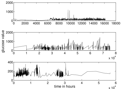
The second data set we utilize includes three patients from the Columbia University Medical Center (CUMC) patient database, containing the records of million individuals over the course of years. We selected these patients by first narrowing the set of patients to those who had glucose time series with at least points so that we could test the bias estimate techniques on the same patient over a wide range of time series lengths. This restricted our population to a few hundred patients. We then calculated the TDMI on the each patient’s full time series as well the first points of the respective patient’s time series. After examining a few hundred of such cases, we selected three patients who were particularly representative of the population. The three patients’ time series of glucose values are shown in Fig. 1, thus displaying the sampling rates, proportion of missing values (which are interpolated as straight lines), and overall clustering and irregularity of measurement times. In particular, notice that: patient one has dense and somewhat uniform sampling over much of the year long record; patient two is more irregularly sampled than patient one, but remains relatively uniformly sampled over the years of the record; and patient three has bursts of measurements followed by large gaps between measurements over the year long record. From this it is clear that not all patients will be able to resolve all time scales.
V.2 TDMI estimation results
First, it is important to understand how the TDMI behaves (e.g., what it can resolved, and to what level of accuracy) as is varied for time series of differing lengths. But, because the accuracy of the TDMI estimate depends fundamentally on the number of pairs of points within a time series that are separated by a given , and because the cardinality of this set depends on both the length of the time series and the relative density of sampling, it can be difficult to understand how to apply the TDMI to a time series. Thus, first we will consider how the TDMI behaves in the context of various time series before considering how the TDMI varies with sampling frequencies and sampling irregularities. Similarly, before considering the ensemble averages of TDMI bias estimates, it is important to understand the variation and variance of these estimates. In particular, it is important to visualize how the TDMI, as a measure of correlation decay, decays to the infinite time asymptotic state that is used in the random permutation bias estimate. Note that for this subsection we reduce the size of the data set from to by taking the first time points in the time series.
V.2.1 Lorenz equations results
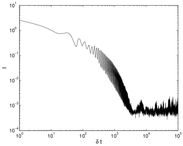
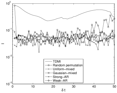
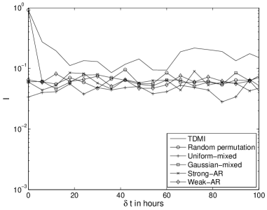
Figure 2 details the TDMI and bias estimates for the Lorenz equations. As can be seen in the long-time plot, nonlinear correlations do not completely dissipate until measurements are separated by at least data points at the given measurement frequency. The raw TDMI estimates for the both the and point strings are identical, certainly up to the bias and error. The TDMI results for the point string, while a qualitatively different raw TDMI graph from the and point estimates, are not wildly different; moreover, the raw TDMI estimated on the point data set is not on the same order of magnitude as any of the bias estimates. Thus, while points may not be enough for an extremely accurate TDMI estimate, it is enough to establish a difference between persistent, existent correlation and bias. The variance of the various bias estimates again appears to follow a power-law in the number of points in a data string — implying that small sample size effects do not dominate the estimate of the estimator bias. And finally, the different bias estimation techniques do not differ enough to cause any difference in interpretation of the TDMI signal; however, the Gaussian-mixed estimate in the presence of long data-strings appears to be an upper bound on other bias estimates.
V.2.2 Glucose results
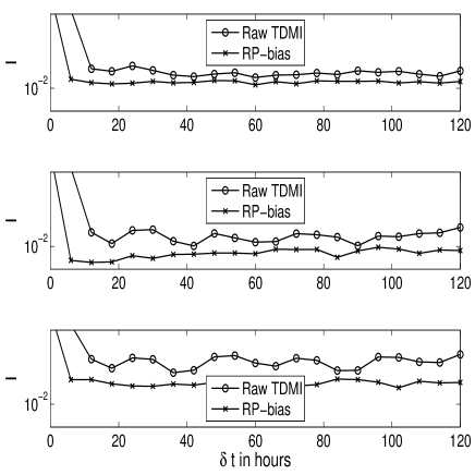
To show that the TDMI, and our bias estimates are not sensitive to sampling frequency or specific source, consider Fig. 3, where the TDMI and random permutation bias is plotted for the three patients. In all cases the bias is below the TDMI signal as expected. Moreover, the bias estimates show relatively little variance, implying that the distribution of bias estimates will be a rather peaked distribution. Note that the each patient has a daily peak in predictability, meaning that points separated by hours are the most predictive of one another aside from points separated by less than hours. However, not all patients have the same magnitude of TDMI peak, meaning, the patients are not all equally predictable. While we hypothesize that this variance in the TDMI daily peaks is related to the relative health of the given patient’s endocrine system, a more detailed discussion is beyond the scope of this paper.
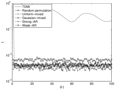
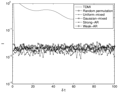
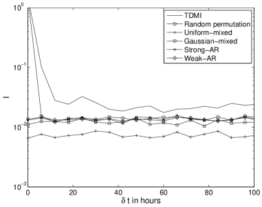
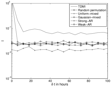
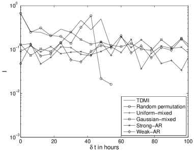
Recall that our goal is to understand how to estimate bias of the TDMI algorithm in a fast, reliable way based on the data. Therefore, to demonstrate and test the TDMI bias estimation algorithms, will focus on patient one, the patient whose TDMI signal is the most difficult to resolve. Figure 4 details the TDMI of the glucose values for patient one. First notice that the and point TDMI results are very similar, including the correlation peak at hours; however, the point TDMI appears to resolve a hour peak as well, implying that the number of points does effect the detail of resolution of a given signal. Moreover, in both the point and the point TDMI calculations, the TDMI signal is never buried in the bias. Nevertheless, there is an important difference between the glucose results and the Lorenz-based results: for the glucose-based results, in general the difference between the TDMI and the bias is smaller when is larger () whereas for the Lorenz-based results the opposite is true. Said simply, the Lorenz-based result produces the expected outcome, whereas the glucose-based result produces a surprise outcome. There are two points to make about the unexpected nature of the glucose-TDMI results for the and data point data sets. First, while the difference between the TDMI and the bias is smaller when is larger, this effect is relatively small and does not change any of the conclusions that can be drawn from either TDMI signal. Second, it is unlikely that this data source is stationary; in particular, this patient had a terminal disease and was slowly failing, and thus we hypothesize that the amount of predictive information in this patient’s signal was likely decreasing (we will not attempt to further justify this hypothesis here). Refocusing on the bias estimates for the and point cases, overall, the various bias estimates yield very similar results (all bias estimates are on the same order of magnitude). Nevertheless, note that here the uniform-mixed is slightly separated from the rest of the bias estimates, whereas for the other examples the Gaussian-mixed was separated from the other estimates.
In contrast to the higher- cases, the TDMI estimate for the point data string rises after or equivalently after two days, and moreover differs qualitatively from the and point TDMI estimates. Thus precise TDMI estimates beyond two days with a resolution of quarter days are unlikely with only points even if the points are sampled relatively evenly in time. Nevertheless, the TDMI estimated on the point data set shows a sharp decay in correlation over the first hours. So, while the TDMI estimated with only points will not resolve perfectly, it will nevertheless retain some gross qualitative features of the higher point analogs. Finally, TDMI estimated using a point data set can resolve nothing; even the raw TDMI is buried in the bias estimates and correlation decay over even the first hours is not present.
V.3 Comparing the fixed point bias estimation methods
Bias estimates are represented by distributions that canonically have at least a mean and variance. Moreover, recall that the bias is a function of the number of points in the sample set and the distribution of those points (this controls the number of empty bins which influences bias). The features of a time series that control the number of points in a given bin are the length of the time series and the sampling frequency (i.e., it is impossible to resolve a TDMI with a time series whose maximum time separation is ). Therefore, in an effort to minimize parameter variation, we will not change the sampling rate and merely change the length of the time series (they have the identical effect, reducing the number of points in given bins).
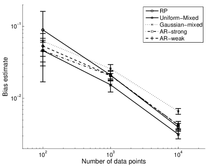
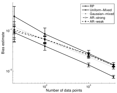
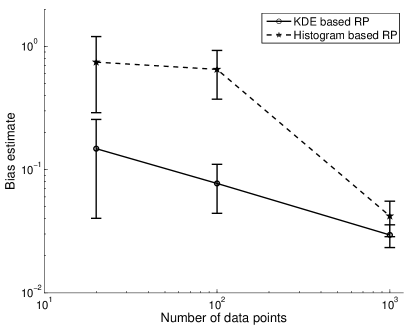
With this in mind, we demonstrate how the permutation-method performs by comparing the mean and variance of the bias estimation methods to one another for different sample sizes, and for different estimators in three steps. First, Fig. 5(a) represents the variation of the bias estimates on a uniformly sampled time series (Lorenz data) of length ; note that such a time-series will have pairs of points in each bin. This figure thus demonstrates how the different bias estimates behave as the absolute number of points use for the PDF estimate varies. In practice, no one characterizes a time series by the number of points separated by a fixed time. Therefore, second, Fig. 5(b) demonstrates the same calculation for the non-uniformly sampled patient one (top plot, Fig. 1). Here again, we do not alter the sampling rate which is already irregular, but merely take the first , , , and points in the time series. This figure demonstrates that the bias estimate methods apply well on real, irregularly time series. Finally, because statistical estimates are made with concrete statistical estimators, Fig. 5(c) demonstrates how the bias estimation methods compare for histogram and KDE PDF estimators.
V.3.1 Summary of conclusions
The broad observations relevant to the KDE-based TDMI bias estimate comparisons include: (a) uniform-mixed bias estimate is usually the lower bound or nearly the lower bound on bias estimates; (b) the Gaussian-mixed bias estimate converges to the uniform-mixed bias estimate in the limit of short data strings and is often an upper bound on all bias estimates for long data strings; (c) the Gaussian-mixed and uniform-mixed bias estimates have the least variance over data string lengths with Gaussian-mixed bias estimates being an upper bound on the uniform-mixed bias estimates; (d) the AR-mixed bias estimates converge to the uniform-mixed bias estimates in the limit of short data strings and often in the limit of a long data strings where the AR-mixed weak bias estimate is always an upper bound on the AR-mixed strong bias estimate; (e) the random-permutation bias estimate progresses from a lower bound bias estimate for long data strings, usually coinciding with the uniform-mixed bias estimate, to an upper bound bias estimate on short data strings; (f) the fixed point bias estimates in all cases roughly obey the dependence on the number of points shown analytically for the histogram estimator; and (g) all of the fixed point bias estimation techniques yield estimates on the same order of magnitude.
V.3.2 Detailed support of conclusions
Observation (a), that the uniform-mixed is always a lower bound on the bias estimates, is expected in light of how information entropy is, in general, maximized [34]. The uniform-mixed bias estimate fits only a single parameter, the mean, to estimate the distribution of the data. Thus the uniform-mixed bias estimate assumes the least possible information regarding the intra-distribution correlations. Said differently, all correlations between subsets of the domain of the distribution are weighted uniformly, thus minimizing the bias estimates in most circumstances. Similarly, observation (b), that the Gaussian-mixed bias estimate converges to the uniform-mixed bias estimate in the limit of few points is largely due to the fact that the Gaussian-mixed bias estimate is dependent on both the mean and variance of the target distribution. Because the variance for distribution with very few points is very similar to the width of the domain of the target distribution, the Gaussian-mixed and uniform-mixed bias estimates nearly coincide. That the Gaussian-mixed bias estimate is an upper bound on other bias estimates for long data strings is related to the fact that the variance of the Gaussian was fixed at one and the entropy of a Gaussian is proportional to the variance. Finally, that the uniform-mixed and Gaussian-mixed bias estimates have the least variance over the length of the data strings is largely due to the fact that their respective marginals are completely independent of the distribution of data. That the AR-mixed bias estimates differ in this regard is due to the fact that the estimated distribution that the random numbers are generated from depends on each data set.
Observation (d), that the AR-mixed bias estimates converge to the uniform-mixed bias estimates in the limits of long and short data strings while remaining below the Gaussian-mixed bias estimates for data strings of intermediate lengths has a simple explanation. In particular, for long data strings, the AR-mixed bias estimate converges to the random-permutation bias estimate because there is enough data for the AR-mixed distribution to reasonably approximate the real data distribution. This essentially verifies that the fixed point method of bias estimation we propose in this work is reasonable because the TDMI estimates from fabricated data from a distribution that resembles the distribution of the original data set coincides with the TDMI results from the randomly permuted data. For short data strings, the AR-mixed bias estimate converges to the uniform bias estimate because with so few points, the AR-mixed distribution that fits the data best is often a uniform distribution as per the principle of maximum entropy.
Observation (e), that the random-permutation bias estimate works well for long data strings and poorly for short data strings, is the result of most practical importance because it implies that using a randomly permuted bias estimate for short data strings may yield an overestimate of the bias. In particular, here when we randomly permute the data string, the permutation is executed without replacement, meaning that the data values are randomly permuted only, never replaced. This means that for a randomized data string of length (or ), the average time separation between permuted values will be (or ). Thus, when is small (say, ), the randomly permuted data set can have a TDMI bias estimate that is actually larger than the raw TDMI estimate because on average, the data pairs are closer in time on average, than for the raw data string. This implies that using a random permutation bias estimate for short data strings will at best grossly overestimate the bias, and at worst will give a bias estimate that will be unusable (e.g., greater than the raw TDMI value). This is the primary reason why we have proposed using the data fabrication techniques for estimating TDMI bias for sparse time series.
Observations (f) and (g) imply that the fixed point bias estimation techniques are both robust in that there is not significant variation across the four techniques and consistent with other analytical estimates of the estimator bias despite the fact that the analytical estimates of bias were calculated for different estimator. In particular, that the bias estimates for KDE and histogram estimators both have the bias dependency is expected given that in the bias estimates between two independent random variables have the bias dependency for both KDE and histogram estimators. Moreover, that all the estimation techniques produce roughly the same results is more surprising and implies that the number of points used for the estimate is the most important variable for the fixed point bias estimation technique. This means that the technique is insensitive to how the time-dependency is removed. Finally, that the fixed point bias estimation techniques are similar to the analytical bias estimates implies what is likely the most important feature: the fixed point bias estimates do approximate the estimator bias accurately.
The estimator-dependent effects on the bias estimates that can be read off Fig. 5(c) include: (i) for small there is a substantial difference between the KDE and histogram TDMI estimates whereas for large they agree; (ii) the histogram estimate is greater than the KDE estimate and has a greater variance (i.e., the histogram TDMI estimate approaches from above while the KDE TDMI estimate approaches from below); (iii) the TDMI fixed point bias estimate of both estimators decreases roughly proportional to ; and (iv), the difference between the small and large TDMI fixed point bias estimate is much smaller for the KDE-based TDMI estimate than for the histogram-based TDMI estimate. This all implies that both the KDE and histogram estimators can be used to estimate the estimator bias in a TDMI calculation; for small sample sizes, the KDE-based calculation appears to work better. Based on how KDE versus histogram estimation schemes work, these results are not surprising. Nevertheless, because there is an estimator dependence on the bias estimate that depends on sample size, comparing results from two estimators can reveal small sample size effects.
The reason why the difference between the KDE and histogram bias estimates can be used to reveal small sample size effects lies in the difference in how they assign probabilities to bins without points in the situation where few bins have any points. The histogram estimator underestimates the probability of bins with few points as it assigns a strict zero if the bin contains no pairs. Thus, histogram estimators, in the presence of small sample sizes, tend to represent sharply peaked distributions. In contrast, the KDE estimator weights each bin (or point relative to its bandwidth) more like a uniform distribution in the presence of few samples. Thus, the KDE estimator tends to represent too smooth a distribution, or a uniform distribution. Therefore, KDE and histogram estimators approach the infinite bias limit from below and above respectively.
VI Summary and discussion
Robust and consistent with previous bias estimate techniques—Based on the analysis in the previous section, we claim that the fixed-point bias estimation method for estimating the TDMI bias is accurate, easy to use, robust with respect to differing methodologies, and works for a variety of estimators. In particular, all the time-dependency removal schemes we employed qualitatively reproduced the bias dependency previously know for histogram estimators and observed in the KDE estimators. Moreover, all the bias estimate schemes we employed are easy to use and compute as fast as the standard TDMI computation. Finally, because the bias estimation technique relies on re-ordering or replacing the data before the PDF estimates are carried out, this estimation scheme will work for all PDF estimators.
Contrasting the bias estimate methods—Given data strings that have a reasonable density and length, the random permutation bias estimate will likely yield both the best estimate of the bias and the fastest implementation of a bias estimate. Nevertheless, for short data strings, the random-permutation bias estimate is likely to overestimate the bias. This overestimate occurs primarily because randomly permuting a few time-correlated points will, on average, force an average maximum time separation of one-third the length of time represented in the data set. For short data-sets, this can imply a significant amount of time-based correlation. Luckily, in the context of short data strings, the uniform-mixed bias estimates do work reasonably well. Moreover, in all data-string length contexts, using more sophisticated means of fabricating data such as accept-reject methods for generating distributions do not, in general, outperform either the uniform-mixed or Gaussian-mixed, or random permutation bias estimates. Because these more sophisticated bias estimation techniques can be significantly more computationally intensive, we do not recommend their implementation.
Data-based constraints on the TDMI calculation—For data sets with fewer than points, very little TDMI related information can be gained. However, for data sets with as few as points, very often qualitative time-based correlation information such as a simple decay in correlation can be determined. As the number of points increase from up to and beyond, the TDMI and TDMI bias calculations continue to improve. For the data sets we considered in this paper, beyond points all of the qualitative and some quantitative conclusions drawn from the TDMI signal did not change when more data points were added. Nevertheless, these statements depend on the density of the data in time, the time-resolution desired, and the uniformity of the measurements in time. Finally, when there is concern about the presence of small sample size effects, a comparison (via the difference) between histogram and KDE-based estimates of the TDMI fixed point bias can be used to detect and quantify the existence of the small sample size effects.
Consequences for data-set aggregation techniques—Finally, because little TDMI information can be gleaned from data strings of lengths shorter than points, and because sparse time series may have fewer than points, the usefulness of utilizing such sparse data for statistical analysis will often hinge on the ability to aggregate like time series into a single long time series. With respect to the TDMI and its bias calculation, for medical data where most patients are similar statistically and thus may be allow for aggregation, but for which the patients all have few points and their individual bias contributions must be handled within patient, it may be best to use fabricated data to estimate the TDMI bias. Or, said differently, for data sets that allow for aggregation, if the bias must be estimated on an intra-string basis, random-permutation bias estimates will likely overestimate the bias. In such cases, we recommend calculating both the random-permutation and the uniform-mixed bias estimates. Contrasting these two bias estimates will likely yield a fruitful interpretation and estimate of the bias.
DJA and GH would like to acknowledge the Columbia University Department of Biomedical Informatics data-mining group for helpful discussions; D. Varn and J. F. S. Dias for a careful reading of the manuscript; and financial support provided by NLM grant RO1 LM06910, an award from Microsoft Research for the Phenotypic Pipeline for Genome-wide Association Studies, and a grant from The Smart Family Foundation.
References
- [1] J. D. Scargle. Studies in astronomical time series analysis ii Statistical aspects of spectral analysis of unevenly spaced data. Astrophys. J., 263:835–853, 1982.
- [2] Y. Ogura and A. Yagihashi. Non-stationary finite-amplitude convection in a thin fluid layer bounded by a stably stratified region. J. Atm. Sci., 28:1389–1399, 1971.
- [3] S. Rutherford, M. E. Mann, T. L. Delworth, and R. J. Stouffer. Climate field reconstruction under stationary and nonstationary forcing. J. Climate, 16:462–479, 2003.
- [4] A. R. Bansal and V. P. Dimri. Depth determination form a non-stationary magnetic profile for scaling geology. Geophysical Propspecting, 53:399–410, 2003.
- [5] M. Schulta and K. Stattegger. Spectrum: Spectral analysis of unevenly spaced paleoclimatic time series. Comput. Geosci., 23:929–945, 1997.
- [6] S. Baisch and G. H. R. Bokelmann. Spectral analysis with incomplete time series: An example form seismology. Comput. Geosci., 25:739–750, 1999.
- [7] P. M. Atkinson. Geographical information science: GeoComputation and nonstationarity. Prog. Phys. Geography, 25:111–122, 2001.
- [8] R. K. Snider and A. B. Bonds. Classification of non-stationary neural signals. J. Neuro. Methods, 84:155–166, 1998.
- [9] E. N. Brown, R. E. Kass, and P. P. Mitra. Multiple neural spike train data analysis: state-of-the-art and future challenges. Nature Neuroscience, 2004.
- [10] Analysis of non-stationary neurobiological signals using empirical mode decomposition. Springer Berlin / Heidelberg, 2008.
- [11] B. Cazelles, M. Chavez, A. J. McMichael, and S. Hales. Nonstationary influence of E] Nino on the synchronous Dengue epidemics in Thailand. PLoS Med., 2:e106, 2005.
- [12] A. W. C. Liew, J. Xian, S. Wu, D. Smith, and H. Yan. Spectral estimation in unevenly sampled space of periodically expressed microarray time series data. BMC Bioinformatics, 8:137–156, 2007.
- [13] M. Jun and M. L. Stein. Nonstationary covariance models for global data. Ann. Appl. Stat., 2:1271–1289, 2008.
- [14] H. Kantz, Kurths J, and G. Mayer-Kress. Nonlinear analysis of physiological data. Springer, 1998.
- [15] T. P. Bronez. Spectral estimate of irregularly sampled multidimensional processes by generalized prolate spheroidal sequences. IEEE Trans. Acoustics, Speech and Signal Processing, 36:1862–1873, 1988.
- [16] P. Babu and P. Stoica. Spectral analysis of nonuniformly sampled data — a review. Digital Signal Process., 2009.
- [17] H. Kantz and T. Schreiber. Nonlinear Time Series Analysis. Cambridge University Press, edition, 2003.
- [18] A. S. Weigend and N. A. Gershenfeld, editors. Time series prediction: Forcasthing the future and understanding the past. Addison Westley, 1994.
- [19] J. C. Sprott. Chaos and Time-series Analysis. Oxford University Press, 2003.
- [20] C, Friedman, A. Wong, and D Blumenthal. Achieving a nationwide learning heath system. Sci. Transl Med, 2:57, 2010.
- [21] D Blumenthal and M Tavenner. The ”meaningful use” regulation for electronic health records. N Engl J Med, 363:501–504, 2010.
- [22] D. J. Albers and G. Hripcsak. Using population scale (ehr) data to understand and test human physiological dynamics. submitted, 2011.
- [23] T. M. Cover and J. A. Thomas. Elements of information theory. Wiley, 1991.
- [24] C. E. Shannon and W. Weaver. The mathematical theory of communication. University of Illinios Press, 1963.
- [25] B. Pompe. Measuring statistical dependencies in a time-series. J. Stat. Phys., 73:587–610, 1993.
- [26] A. M. Fraser and H. L. Swinney. Independent coordinates for strange attractors from mutual information. Phys. Rev. A, 33:1134–1140, 1986.
- [27] A. Kraskov, H. Stögbauer, and P. Grassberger. Estimating mutual information. Phys. Rev. E, 2004.
- [28] Y-I Moon, B. Rajagopalan, and U. Lall. Estimation of mutual information using kernel density estimators. Phys. Rev. E, 52:2318 – 2321, 1995.
- [29] Gray and Moore. Very fast multivariate kernel density estimation using via computational geometry. In Joint Stat. Meeting, 2003.
- [30] G. P. Basharin. On a statistical estimate for entropy of a sequences of independent random variables. Theory Prop. App., 4:333–338, 1959.
- [31] M. S. Roulston. Estimating the errors on measured entropy and mutual information. Physica D, 125:285–294, 1999.
- [32] P. Grassberger. Finite sample corrections to entropy and dimension estimates. Phys. Lett. A, 128:369–373, 1988.
- [33] E. N. Lorenz. Deterministic nonperiodic flow. J. Atmosph. Sci., 20:130–141, 1963.
- [34] E. T. Jaynes. Information theory and statistical mechanics. Phys. Rev, 106:620, 1957.