Abstract

Rift Valley fever is a vector-borne zoonotic disease which causes high morbidity and mortality in livestock. In the event Rift Valley fever virus is introduced to the United States or other non-endemic areas, understanding the potential patterns of spread and the areas at risk based on disease vectors and hosts will be vital for developing mitigation strategies. Presented here is a general network-based mathematical model of Rift Valley fever. Given a lack of empirical data on disease vector species and their vector competence, this discrete time epidemic model uses stochastic parameters following several PERT distributions to model the dynamic interactions between hosts and likely North American mosquito vectors in dispersed geographic areas. Spatial effects and climate factors are also addressed in the model. The model is applied to a large directed asymmetric network of $3,621$ nodes based on actual farms to examine a hypothetical introduction to some counties of Texas, an important ranching area in the United States of America (U.S.A.). The nodes of the networks represent livestock farms, livestock markets, and feedlots, and the links represent cattle movements and mosquito diffusion between different nodes. Cattle and mosquito (Aedes and Culex) populations are treated with different contact networks to assess virus propagation. Rift Valley fever virus spread is assessed under various initial infection conditions (infected mosquito eggs, adults or cattle). A surprising trend is fewer initial infectious organisms result in a longer delay before a larger and more prolonged outbreak. The delay is likely caused by a lack of herd immunity while the infections expands geographically before becoming an epidemic involving many dispersed farms and animals almost simultaneously. Cattle movement between farms is a large driver of virus expansion, thus quarantines can be efficient mitigation strategy to prevent further geographic spread.

Introduction

Rift Valley fever (RVF) was first identified in Egypt in $1931$ [1] and is endemic in the eastern and southern regions of Africa [2]. Viral infection may result in abortion in adults and death in newborn livestock [3]. Sheep, goats and cattle are the most important domestic animal hosts affected when viewed from an economic standpoint [2] although humans also can become infected [4, 3].

Aedes and Culex genera of mosquitoes are thought to be main RVF disease vectors with respect to vector competence [4]. The virus is maintained between epidemics through vertical transmission within the Aedes mosquitoes [5], and is thought to be propagated and amplified during epidemics by both Aedes and Culex species mosquitoes. High RVF transmission is typically related to persistent, above average rainfall and El Niño/Southern Oscillation (ENSO) events in Eastern Africa which create favorable mosquito habitats [6]. Aedes mosquitoes lay eggs in dry mud [7] and the eggs can survive for long periods of time [2]. After flooding, RVF virus-infected eggs can develop into infected adult mosquitoes [2]. Infected adult Aedes mosquitoes then feed on animals which become infected, and spread the infection to other Aedes and Culex genera adult mosquitoes feeding on infected animals.

Animal movements, typically motivated by livestock trading and marketing may accelerate the transmission of zoonotic diseases among animal holdings which may cover a vast area [8]. In $1977$, the trade of sheep from east Africa during Ramadan was considered to be a likely pathway for the introduction of RVF virus to Egypt [9, 10, 11]. A boy from Anjouan, an island of Comoros archipelago, was diagnosed to have been infected with RVF virus on the French island of Mayotte in $2007$ [4]. The Rift Valley fever virus was likely to be introduced by live ruminants imported from Kenya or Tanzania in the trade during the 2006-2007 Rift Valley fever outbreak [4].

Humans can acquire the infection from the bites of infected mosquitoes or directly from contact with the bodily fluids of infected animals [12]. Individuals working with animals, such as farmers and veterinarians, are the most vulnerable to RVF virus infection during animal outbreaks[13] because of increased exposure to mosquitoes in an outdoor environment and direct contact with animals. Rift Valley fever virus infection causes severe influenza-like disease in humans with serious consequences such as blindness, or even death [3]. It has been reported that more than $200$ persons died of RVF in Mauritania in $1987$ [14]. There were $738$ reported human cases in Sudan, including $230$ deaths, in $2007-2008$ [15]. It is likely that the number of human cases has been underreported in the past, especially in rural areas [4]. Rift Valley fever virus has spread outside of Africa to Yemen and Saudi Arabia in $2000$ [4] and the French island of Mayotte with multiple human cases reported [16]. Rift Valley fever virus could possibly be introduced to the United States, similar to the experience with West Nile virus which was introduced into the North America in $1999$ [17]. A mathematical epidemiological model can be applied to non-traditional locations in order to study the potential for spatial spread of RVF virus.

Epidemiological modeling plays an important role in planning, implementing, and evaluating detection, control, and prevention programs [18]. Mathematical modeling takes the advantage of economic, clear and precise mathematical formulation, e.g., applications of differential, integral, or functional differential equations [18]. Mathematical models of infection transmission include interpretation of transmission processes and are often useful in answering questions that cannot be answered only with empirical data analysis [19], as well as to explore biological and critical ecological characteristics of disease transmission [20, 21]. Current RVF virus transmission models are useful in representing infection transmission process [19] but are limited in determining and testing relevant risk factors. For the Ferlo area of Senegal, a pond-level meta-population model which considered only vectors was developed assuming that Aedes mosquitoes were the only vector and rainfall was the only driving force [2]. It has been shown that within Ferlo, the virus would persist only if the livestock moved between ponds and the rainfall did not occur in all ponds simultaneously [2]. Very few mathematical dynamic transmission models have explored mechanisms of RVF virus circulation [19] on a larger geographical scale. A theoretical model in a closed system including Aedes and Culex mosquitoes and livestock population was earlier proposed [22]. The key result was that RVF virus can persist in a closed system for $10$ years if the contact rate between hosts and vectors is high [19, 22]. Another theoretical RVF virus transmission mathematical model [23] modified the model in [22] by adding human hosts, merging all mosquitoes into one class, removing mosquito egg compartment, as well as vertical transmission of mosquitoes. Sensitivity indices of the reproduction number are used to determine the most sensitive parameters to the basic reproduction number of RVF virus transmission [23]. It has been found that both the reproduction number and disease prevalence in mosquitoes are sensitive to mosquito death rate and the disease prevalence in livestock and humans are more sensitive to livestock and human recruitment rates [23]. A theoretical ordinary differential equation meta-population involving livestock and human mobility was presented [24]. They analyzed the likelihood of pathogen establishment and provided hypothesized examples to illustrate the methodology [24]. A three-patch model for the process by which animals enter Egypt from Sudan, are moved up the Nile, and then consumed at population centers is proposed [25]. Using [22] and [23] as a foundation, the homogeneous models have been extended to a meta-population differential equation model including Aedes, Culex, livestock, and humans and a case study was carried out for South Africa during a country-wide outbreak in 2010 [26]. The model was based on RVF virus spatial transmission during an outbreak, where a network with three nodes corresponding to three affected provinces in South Africa was established. To make the output of the model [26] easily compared with incidence data if available and the simulation for thousands of nodes easily implemented, a discrete time epidemic model is developed and a much larger network on which to study the dynamics of the larger system is established.

Proposed here is a deterministic network-based RVF virus transmission model with stochastic parameters. Two competent vector populations: Aedes mosquitoes, Culex mosquitoes, and two host populations: cattle and humans are considered. The dynamical behavior of mosquito and livestock populations are modeled using a meta-population approach based on weighted contact networks. The nodes of the networks represent geographical locations, and the weights represent the level of contact between regional pairings. In particular, nodes represent different farm sizes or operator businesses of the cattle industry, nominally markets and feedlots. Heterogeneous aspects of the spreading are considered in the model through realistic modeling of the cattle movement among different nodes of the network. Additionally, the mosquito population and development is modeled as a function of climatic factors, such as humidity and temperature. It is easy to implement simulations of the model even for networks with thousands of nodes, and it is easy to compare the output of the model with incidence data if available. The role of starting location has been shown to be important in the final size of rinderpest epidemic [27]. To investigate the role of starting location, and the size of initial infection in RVF virus spread, the proposed model has been applied to a case study to some counties in Texas, U.S. and the model outcomes (the human and cattle cases, and the timing of the epidemic’s characteristics) indicate which biotic factors will play an important role if RVF virus is introduced to the United States.

Methods and Materials

Network-based Meta-population Models

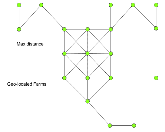
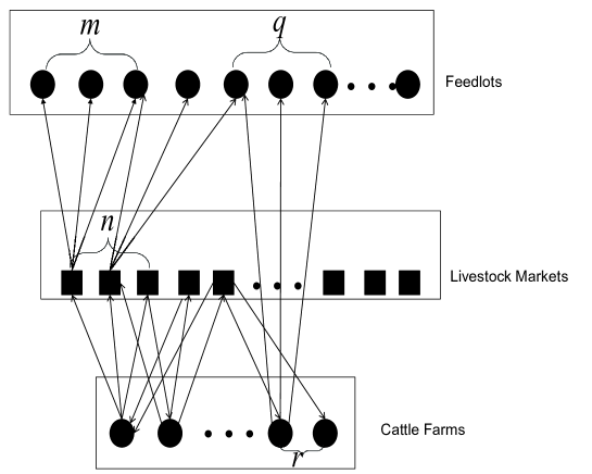
Aedes mosquitoes, Culex mosquitoes, livestock, and human populations each are considered in the network-based meta-population models. The movement of each population is represented by networks, where nodes denote locations, and links denote movement flow between locations. In the mosquito diffusion network, the nodes represent farms and the links represent mosquito diffusion from one farm to the neighboring farms. The weights are diffusion rates $\omega_{1ij}$ for Aedes population, and $\omega_{3ij}$ for Culex population from location $i$ to location $j$. In the livestock movement network, the nodes represent farms, livestock markets, and feedlots. The links represent livestock movements due to livestock trade between the nodes and the weight is the movement rate $\omega_{2ij}$ from node $i$ to node $j$. The mosquito and livestock networks are shown in Fig. 1(a) and Fig. 1(b), respectively.

The compartmental models are adapted to represent the status of each population during a simulated RVF virus transmission. The models are built based on the principle of the RVF virus transmission flow diagram illustrated in [26]. Adult Aedes and Culex populations are distributed among susceptible $S_{ai}$, exposed $E_{ai}$, and infected $I_{ai}$ compartments. Only those mosquito species that are known to be competent vectors of RVF virus transmission are considered and they are broadly grouped by Aedes and Culex genera mosquitoes. The subscript $a=1$ denotes Aedes in node $i$, and $a=3$ denotes Culex mosquitoes in node $i$. Uninfected and infected mosquitoes eggs are represented by $P_{ai}$ and $Q_{ai}$, respectively. Culex mosquitoes do not display vertical transmission. Therefore, only uninfected Culex eggs are incorporated in the model. The livestock and human hosts are likewise considered $S_{bi}$, $E_{bi}$, $I_{bi}$, and $R_{bi}$. The subscript representing livestock in node $i$ is $b=2$, and humans in node $i$ are represented with $b=4$. The descriptions of the parameters in the models are found in Table 1. All the transitions to be discussed below are for location $i$ at day $t$.

(a) An example of mosquito diffusion network

(b) An example of livestock movement network

Figure 1: Mosquito diffusion and livestock movement illustration

Aedes Population Model

$$P_{1i}(t+1)-P_{1i}(t) =b_{1}(N_{1i}(t)-q_{1}I_{1i}(t))-\theta_{1}P_{1i}(t))$$ (1)

$$Q_{1i}(t+1)-Q_{1i}(t) =b_{1}q_{1}I_{1i}(t)-\theta_{1}Q_{1i}(t)$$ (2)

$$S_{1i}(t+1)-S_{1i}(t) =\theta_{1}P_{1i}(t)+\sum^{n}_{j=1,j\neq i}\omega_{1ji}S_{1j}(t)-\sum^{n}_{j=1,j\neq i}\omega_{1ij}S_{1i}(t)-d_{1}S_{1i}(t)N_{1i}(t)/K_{1}$$

$$-\beta_{21}S_{1i}(t)I_{2i}(t)/N_{2i}(t)$$ (3)

$$E_{1i}(t+1)-E_{1i}(t) =\sum^{n}_{j=1,j\neq i}\omega_{1ji}E_{1j}(t)-\sum^{n}_{j=1,j\neq i}\omega_{1ij}E_{1i}(t)-d_{1}E_{1i}(t)N_{1i}(t)/K_{1}+\beta_{21}S_{1i}(t)I_{2i}(t)/N_{2i}(t)$$

$$-\varepsilon_{1}E_{1i}(t)$$ (4)

$$I_{1i}(t+1)-I_{1i}(t) =\sum^{n}_{j=1,j\neq i}\omega_{1ji}I_{1j}(t)-\sum^{n}_{j=1,j\neq i}\omega_{1ij}I_{1i}(t)+\theta_{1}Q_{1i}(t)-d_{1}I_{1i}(t)N_{1i}(t)/K_{1}$$

$$+\varepsilon_{1}E_{1i}(t)$$ (5)

$$N_{1i}(t+1) =S_{1i}(t+1)+E_{1i}(t+1)+I_{1i}(t+1)$$ (6)

There are $b_{1}N_{1i}(t)$ eggs laid, including $b_{1}q_{1}I_{1i}(t)$ infected eggs, and $b_{1}N_{1i}(t)-b_{1}q_{1}I_{1i}(t)$ uninfected eggs each day. After the development period, $\theta_{1}P_{1i}(t)$ uninfected eggs develop into susceptible adult Aedes mosquitoes and $\theta_{1}Q_{1i}(t)$ infected eggs develop into infected adult Aedes mosquitoes. The number of Aedes mosquitoes infected by livestock is $\beta_{21}S_{1i}(t)I_{2i}(t)/N_{2i}(t)$. Following the incubation period, $\varepsilon_{1}E_{1i}(t)$ Aedes mosquitoes transfer from exposed compartment to infected compartment. The number of Aedes mosquitoes dying naturally in compartment $X$ is given as $d_{1}X_{1i}(t)$. The percentage of Aedes mosquitoes moving from location $i$ to location $j$ is $\omega_{1ij}$. The change in the number of Aedes mosquitoes due to mobility in compartment $X$ is given as $\sum^{n}_{j=1,j\neq i}\omega_{1ji}X_{1j}(t)-\sum^{n}_{j=1,j\neq i}\omega_{1ij}X_{1i}(t)$ [28].

Culex Population Model

$$P_{3i}(t+1)-P_{3i}(t) =b_{3}(t)N_{3i}(t)-\theta_{3}(t)P_{3i}(t)$$ (7)

$$S_{3i}(t+1)-S_{3i}(t) =\theta_{3}(t)P_{3i}(t)+\sum^{n}_{j=1,j\neq i}\omega_{3ji}S_{3j}(t)-\sum^{n}_{j=1,j\neq i}\omega_{3ij}S_{3i}(t)-d_{3}S_{3i}(t)N_{3i}(t)/K_{3}$$

$$-\beta_{23}S_{3i}(t)I_{2i}(t)/N_{2i}(t)$$ (8)

$$E_{3i}(t+1)-E_{3i}(t) =\sum^{n}_{j=1,j\neq i}\omega_{3ji}E_{3j}(t)-\sum^{n}_{j=1,j\neq i}\omega_{3ij}E_{3i}(t)-\varepsilon_{3}E_{3i}(t)-d_{3}E_{3i}(t)N_{3i}(t)/K_{3}$$

$$+\beta_{23}S_{3i}(t)I_{2i}(t)/N_{2i}(t)$$ (9)

$$I_{3i}(t+1)-I_{3i}(t) =\sum^{n}_{j=1,j\neq i}\omega_{3ji}I_{3j}(t)-\sum^{n}_{j=1,j\neq i}\omega_{3ij}I_{3i}(t)+\varepsilon_{3}E_{3i}(t)-d_{3}I_{3i}(t)N_{3i}(t)/K_{3}$$ (10)

$$N_{3i}(t+1) =S_{3i}(t+1)+E_{3i}(t+1)+I_{3i}(t+1)$$ (11)

There are $b_{3}N_{3i}(t)$ eggs laid each day. After the development period, $\theta_{3}P_{3i}(t)$ eggs develop into susceptible adult Culex mosquitoes. After the incubation period, $\varepsilon_{3}E_{3i}(t)$ Culex mosquitoes transfer to infected compartment $I$. The number of Culex mosquitoes acquiring infection from livestock is denoted by $\beta_{23}S_{3i}(t)I_{2i}(t)/N_{2i}(t)$. The Culex mosquitoes removed from compartment $X$ due to natural death is $d_{3}X_{3i}(t)$. The percentage of Culex mosquitoes moving from location $i$ to location $j$ is $\omega_{3ij}$. The change in the number of Culex mosquitoes due to movement in compartment $X$ is given as $\sum^{n}_{j=1,j\neq i}\omega_{3ji}X_{3j}(t)-\sum^{n}_{j=1,j\neq i}\omega_{3ij}X_{3i}(t)$ [28].

Livestock Population Model

$$S_{2i}(t+1)-S_{2i}(t) =b_{2}(t)\delta_{b}(i)N_{2i}(t)+\sum^{n}_{j=1,j\neq i}\omega_{2ji}S_{2j}(t)-\sum^{n}_{j=1,j\neq i}\omega_{2ij}S_{2i}(t)-d_{2}\delta_{d}(i)S_{2i}(t)N_{2i}(t)/K_{2}$$

$$-\beta_{12}S_{2i}(t)I_{1i}(t)/N_{1i}(t)-\beta_{32}S_{2i}(t)I_{3i}(t)/N_{3i}(t)$$ (12)

$$E_{2i}(t+1)-E_{2i}(t) =\sum^{n}_{j=1,j\neq i}\omega_{2ji}E_{2j}(t)-\sum^{n}_{j=1,j\neq i}\omega_{2ij}E_{2i}(t)-d_{2}\delta_{d}(i)E_{2i}(t)N_{2i}(t)/K_{2}-\varepsilon_{2}E_{2i}(t)$$

$$+\beta_{12}S_{2i}(t)I_{1i}(t)/N_{1i}(t)+\beta_{32}S_{2i}(t)I_{3i}(t)/N_{3i}(t)$$ (13)

$$I_{2i}(t+1)-I_{2i}(t) =p\sum^{n}_{j=1,j\neq i}\omega_{2ji}I_{2j}(t)-p\sum^{n}_{j=1,j\neq i}\omega_{2ij}I_{2i}(t)-d_{2}\delta_{d}(i)I_{2i}(t)N_{2i}(t)/K_{2}+\varepsilon_{2}E_{2i}(t)$$

$$-\gamma_{2}I_{2i}(t)-\mu_{2}I_{2i}(t)$$ (14)

$$R_{2i}(t+1)-R_{2i}(t) =\sum^{n}_{j=1,j\neq i}\omega_{2ji}R_{2j}(t)-\sum^{n}_{j=1,j\neq i}\omega_{2ij}R_{2i}(t)+\gamma_{2}I_{2i}(t)-d_{2}\delta_{d}(i)R_{2i}(t)N_{2i}(t)/K_{2}$$ (15)

$$N_{2i}(t+1) =S_{2i}(t+1)+E_{2i}(t+1)+I_{2i}(t+1)+R_{2i}(t+1)$$ (16)

The daily number of newborn livestock in location $i$ is $b_{2}(t)N_{2i}(t)$. The variables $\delta_{b}(i)$ and $\delta_{d}(i)$ are used to differentiate different types of nodes. If location $i$ is a farm, then $\delta_{b}(i)=1$, $\delta_{d}(i)=1$. If location $i$ is a market, then $\delta_{b}(i)=0$, $\delta_{d}(i)=0$. If location $i$ is a feedlot, then $\delta_{b}(i)=0$, $\delta_{d}(i)=1$. The numbers of livestock infected by Aedes mosquitoes and Culex mosquitoes are denoted by $\beta_{12}S_{2i}(t)I_{1i}(t)/N_{1i}(t)$ and $\beta_{32}S_{2i}(t)I_{3i}(t)/N_{3i}(t)$, respectively. After the incubation period, $\varepsilon_{2}E_{2i}(t)$ livestock transfer from exposed state to infected state. After the infection period, $\gamma_{2}I_{2i}(t)$ livestock recover from RVF virus infection. The number of dead livestock in compartment $X$ is given as $d_{2}X_{2i}N_{2i}(t)/K_{2}$ in which $K_{2}$ is the carrying capacity of livestock in each node. The change in the number of livestock in compartment $X$ due to mobility is given as $\sum^{n}_{j=1,j\neq i}\omega_{2ji}X_{2j}(t)-\sum^{n}_{j=1,j\neq i}\omega_{2ij}X_{2i}(t)$ for livestock in compartments $S$, $E$, and $R$, and $p\sum^{n}_{j=1,j\neq i}\omega_{2ji}X^{[m]}_{2j}(t)$-$p\sum^{n}_{j=1,j\neq i}\omega_{2ij}X^{[m]}_{2i}(t)$ [28], $(0<p<1)$ for livestock in compartment $I$.

Human Population Model

$$S_{4i}(t+1)-S_{4i}(t) =-\beta_{14}S_{4i}(t)I_{1i}(t)/N_{1i}(t)-\beta_{24}S_{4i}(t)I_{2i}(t)/N_{2i}(t)-\beta_{34}S_{4i}(t)I_{3i}(t)/N_{3i}(t)$$ (17)

$$E_{4i}(t+1)-E_{4i}(t) =\beta_{14}S_{4i}(t)I_{1i}(t)/N_{1i}(t)+\beta_{24}S_{4i}(t)I_{2i}(t)/N_{2i}(t)+\beta_{34}S_{4i}(t)I_{3i}(t)/N_{3i}(t)$$

$$-\varepsilon_{4}E_{4i}(t)$$ (18)

$$I_{4i}(t+1)-I_{4i}(t) =\varepsilon_{4}E_{4i}(t)-\gamma_{4}I_{4i}(t)$$ (19)

$$R_{4i}(t+1)-R_{4i}(t) =\gamma_{4}I_{4i}(t)$$ (20)

The number of humans in each node is constant because birth, death, mortality, and mobility of humans are not considered. The number of humans infected by Aedes mosquitoes, Culex mosquitoes, and livestock is $\beta_{14}S_{4i}(t)I_{1i}(t)/N_{1i}(t)$, $\beta_{24}S_{4i}(t)I_{2i}(t)/N_{2i}(t)$, and $\beta_{34}S_{4i}(t)I_{3i}(t)/N_{3i}(t)$, respectively. There are $\varepsilon_{4}E_{4i}(t)$ humans transferring to infected compartment after incubation period, and $\gamma_{4}I_{4i}(t)$ humans recovering from RVF virus infection after infection period.

Table 1: Parameter ranges for numerical simulations.

Parameter	Description	Range	Assumed most possible value	Units	Source
$\beta_{12}$	contact rate: Aedes to livestock	$(0.0021,0.2762)$	0.1392	$1/$day	[29, 30, 31, 32, 33, 34, 35]
$\beta_{21}$	contact rate: livestock to Aedes	$(0.0021,0.2429)$	0.1225	$1/$day	[29, 30, 31, 32, 33, 36]
$\beta_{23}$	contact rate: livestock to Culex	$(0.0000,0.3200)$	0.16	$1/$day	[30, 31, 32, 33, 36, 37]
$\beta_{32}$	contact rate: Culex to livestock	$(0.0000,0.096)$	0.04	$1/$day	[30, 31, 32, 33, 37]
$\beta_{14}$	contact rate: Aedes to humans	$(0.001,0.002)$	0.0015	$1/$day	Assume
$\beta_{24}$	contact rate: livestock to humans	$(0.00004,0.00008)$	0.00006	$1/$day	Assume
$\beta_{34}$	contact rate: Culex to humans	$(0.0005,0.001)$	0.000525	$1/$day	Assume
$1/\gamma_{2}$	recovery period in livestock	$(2,5)$	3.5	$1/$day	[38]
$1/\gamma_{4}$	recovery period in humans	$(4,7)$	5.5	$1/$day	[23]
$1/d_{1}$	longevity of Aedes mosquitoes	$(3,60)$	31.5	days	[39, 40, 33]
$1/d_{2}$	longevity of livestock	$(360,3600)$	1980	days	[41]
$1/d_{3}$	longevity of Culex mosquitoes	$(3,60)$	31.5	days	[39, 40, 33]
$b_{1}$	birth rate of Aedes mosquitoes	weather dependent		$1/$day	[39, 40, 33]
$b_{2}$	birth rate of livestock	$d_{2}$		$1/$day	[41]
$b_{3}$	birth rate of Culex mosquitoes	weather dependent		$1/$day	[39, 40, 33]
$1/\epsilon_{1}$	incubation period in Aedes mosquitoes	$(4,8)$	6	days	[34]
$1/\epsilon_{2}$	incubation period in livestock	$(2,6)$	4	days	[42]
$1/\epsilon_{3}$	incubation period in Culex mosquitoes	$(4,8)$	6	days	[34]
$1/\epsilon_{4}$	incubation period in humans	$(2,6)$	4	days	[23]
$\mu_{2}$	mortality rate in livestock	$(0.025,0.1)$	0.0375	$1/$day	[38, 42]
$q_{1}$	transovarial transmission rate in Aedes mosquitoes	$(0,0.1)$	0.05	$1/$day	[43]
$1/\theta_{1}$	development period of Aedes mosquitoes	weather dependent		days	[33]
$1/\theta_{3}$	development period of Culex mosquitoes	weather dependent		days	[44]
$K_{1}$	carrying capacity of Aedes mosquitoes		$100000000$		Assume
$K_{2}$	carrying capacity of livestock		$1000000$		Assume
$K_{3}$	carrying capacity of Culex mosquitoes		$100000000$		Assume
$p$	reduction in $\omega_{2ij}$ due to infection		$\frac{1}{2}$		Assume

Case Study: Texas, U.S.A from $2005$ to $2010$

Networks in the Study Area

As a case study, various RVF virus introduction scenarios were tested using the model to determine the hypothetical model outcomes (number of livestock cases and timing of the epidemic). Although the model accounts for their exact locations when simulating RVF virus spread, we do not report any of this information or even discuss ranches in areas smaller than county level. The exact farms and counties are very well masked from the results. Texas cattle ranches were selected because they have large cattle concentrations and we have aggregate survey data on cattle movements in these areas [45]. A network with $3,526$ cattle farms [46], $3$ livestock markets [46], and $92$ cattle feedlots [46] is constructed. The cattle farms, and livestock markets are located in one region, and the feedlots are in another region. The location of each node is uniformly distributed in each county according to the total number of farms within each county [46]. The exact location of each farm is obscured because those data are not publicly available [47] due to confidentiality. The initial number of cattle in each farm is categorized as $0-9$, $10-19$, $20-49$, $50-99$, $100-199$, $200-499$ and more than $500$ [46]. The initial number of susceptible cattle in each farm or feedlot for numerical simulation is assumed according to the number of cattle in each county in $2007$ [46] and the histogram of the number of cattle [46]. For cattle movement, if cattle are sold from one node to another, then there is a link between the nodes. The movement rate of cattle denoted by $\omega_{2ij}$ shown in Table 2 is estimated based on the aggregate movement rates from survey [45] and inversely proportional to the distance between source-destination pairs. Movement rate is the average movement rate for all cattle at different ages, and the movement rate of cattle in compartment $I$ is assumed to be half the movement rate for cattle in compartments S, E, and R, namely, $p=\frac{1}{2}$

Table 2: Cattle movement rate $\omega_{2ij}$, where $n_{m}(i)$=the number of markets connected to farm $i$, $n_{f}(i)$=the number of farms connected to market $i$, $n_{ffe}(i)$=the number of feedlots connected to farm $i$, $n_{mfe}(i)$=the number of feedlots connected to market $i$.

$\mathbf{i}$	$\mathbf{j}$	Range	Source
farm	market	$60.7\%$ /$(n_{m}(i)\times d_{ij})$	[45]
market	farm	$60.7\%$ /$(n_{f}(i)\times d_{ij})$	[45]
farm	feedlot	$10.9\%$ /$(n_{ffe}(i)\times d_{ij})$	[45]
market	feedlot	$10.9\%$ /$(n_{mfe}(i)\times d_{ij})$	[45]
feedlot	farm	$0$	[45]
feedlot	market	$0$	[45]

For mosquito diffusion, if the distance between two farms is smaller than an assumed radius, two kilometers, then there is a link between the nodes in the network. The diffusion rates of Aedes and Culex mosquitoes are shown below [48].

$$\omega_{1ij}=\omega_{3ij}=\left\{\begin{array}[]{l l}0,&\quad\text{ if the nodes are disjoint}\\ diff/d_{ij}^{2},&\quad\text{if two nodes share a border}\\ \end{array}\right.$$

where $d_{ij}$is the distance between the centers of node $i$ and node $j$ [48] and $diff$ is a diffusion like parameter within the range $(830,8300)m^{2}/$day [48].

Parameters for Numerical Simulations

Vector competence varies within and between mosquito species [49]. Stochastic parameters were used to account for broad range of vector competence between Aedes and Culex species and individual variation within each species. The PERT distribution has few constraints (minimum, maximum, and most likely value), similarly to the triangular distribution applied in [50] to simulate West Nile virus epidemic. In the following simulations, PERT distributions are selected to generate stochastic parameters with ranges and the most likely values listed in Table 1. Any appropriate parameter distribution can be adapted into the model.

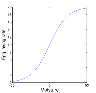
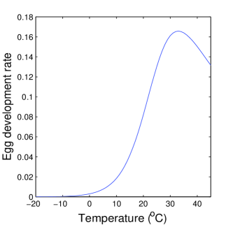
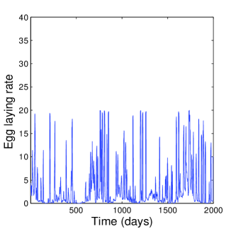
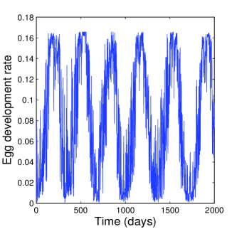
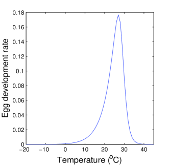
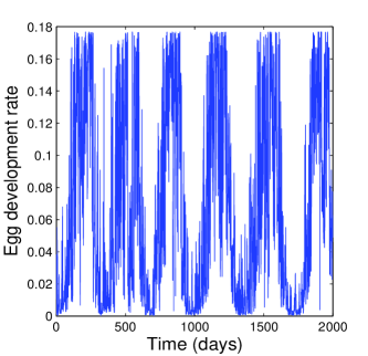
The egg laying rates of Aedes and Culex mosquitoes changing with moisture conditions as indicated in Equation (21) [44] are shown in Fig. 2(a). The egg development rate of Aedes mosquitoes varying with temperature in Equation $(\ref{equation:theta1})$ [51] and that of Culex mosquitoes in Equation $(\ref{equation:developmentrate})$ are in Fig. 2(e) and Fig. 2(b), respectively. The parameters for egg laying rates of Aedes mosquitoes and Culex mosquitoes, and parameters for egg development rate of Culex mosquitoes are derived from data concerning West Nile virus in $2010$ in the Northern U.S. [44], and the parameters for the egg development rate of Aedes mosquitoes is derived using the model for Aedes aegypti [51], which are the best models currently available. More precise parameters can be adopted, as they become available. The egg laying rate of Aedes and Culex mosquitoes, egg development rate of Culex mosquitoes, and egg development rate of Aedes mosquitoes computed with the climate data for the region where cattle farm and markets located in the study area of Texas from January, $2005$ to October, $2010$, are shown in Fig. 2(c), Fig. 2(d), and Fig. 2(f), respectively. If the temperature is too low, the eggs will not develop into larvae and then adult mosquitoes. If the temperature is too high, the lifespan of the mosquitoes is shortened and the development rate decreases. Moisture index is the difference between precipitation and evaporation as shown in Equation (22). A lower moisture index correlates to fewer adult mosquitoes because low moisture index represents a combination of low precipitation and high evaporation. For some days, the missing precipitation data from January, $2005$ to December, $2010$ [52] are assumed to be zero. The evaporation data are calculated using Equation (23) [53]. The parameters in Equations (21) through (25) are listed in Table 4. Although humans move between nodes, they do not transmit virus between nodes and the number of humans in each node (i.e., farm) is assumed to be fewer than $15$.

$$b_{1}(Temp,precipitation,T_{d},t) =b_{3}(Temp,precipitation,T_{d},t)=b_{0}+\frac{Emax}{1+exp[-\frac{Moisture(t)-Emean}{Evar}]},$$ (21)

$$Moisture(t) =\sum^{t}_{D=t-6}precipitation(D)-Evaporation(D),$$ (22)

$$Evaporation(t) =\frac{700(Temp(t)+0.006h)/(100-latitude)}{80-Temp(t)}$$

$$+\frac{15(Temp(t)-T_{d}(t))}{80-Temp(t)},$$ (23)

$$\theta_{1}(Temp,t) =A_{1}*\frac{(Temp(t)+K)}{298.15}*\frac{exp[\frac{HA_{1}}{1.987}*(\frac{1}{298.15}-\frac{1}{Temp(t)+K})]}{1+exp[\frac{HH_{1}}{1.987}*(\frac{1}{TH_{1}}-\frac{1}{Temp(t)+K})]},$$ (24)

$$\theta_{3}(Temp,t) =A*\frac{(Temp(t)+K)}{298.15}*\frac{exp[\frac{HA}{1.987}*(\frac{1}{298.15}-\frac{1}{Temp(t)+K})]}{1+exp[\frac{HH}{1.987}*(\frac{1}{TH}-\frac{1}{Temp(t)+K})]},$$ (25)

where
$Temp(t)=$air temperature in units of ${}^{o}C$ [53]
$latitude=$the latitude (degrees) [53]
$T_{d}(t)=$the mean dew-point in units of ${}^{o}C$ [53]
$h=$the elevation (meters) [53]
$K=$Kelvin parameter

(a) The egg development rate of Culex mosquitoes with temperature [44].

(b) The egg development rate of Culex mosquitoes with temperature [44].

(c) The egg laying rates of Aedes and Culex mosquitoes in the nine counties in the south of Texas from January, $2005$ to October, $2010$.

(d) The egg development rate of Culex mosquitoes in the nine counties in the south of Texas from January, $2005$ to October, $2010$.

(e) The egg development rate of Aedes mosquitoes with temperature.

(f) The egg development rate of Aedes mosquitoes in the nine counties in the south of Texas from January, $2005$ to October, $2010$.

Figure 2: The relationship between egg laying rates, egg development rates of mosquitoes and climate factors.

Results

The Novel Mathematical Model

Presented is a discrete time compartmental mathematical model based on a network approach. Rift Valley fever is transmitted by several species of mosquito vectors that have varying levels of vector competence; therefore, each genus and species combination requires modeling the vector competence, movement, and life stage development patterns which is too complicated while considering only a single species or genus is not accurate. Consequently, the species are loosely grouped as their genera and the parameters are allowed to vary following PERT distributions. The distribution captures uncertainties on inherent variability between species, as well as variability among individual mosquitoes. The mosquito parameters are functions of climate factors to reflect the impact of climate and season on mosquito dynamics. Only Aedes and Culex genera mosquitoes that are competent vectors of RVF virus transmission are considered in the model.

Different networks are developed for mosquito diffusion and livestock movement considering heterogeneity in both. In the cattle movement network, different types of nodes distinguish between sources, sinks, and transitions.

The model can be used to simulate networks with the number of nodes up to thousands with the easily solvable discrete time model. To use the model in any location, one only needs the initial populations, the movement rates, ranges of the parameters, and climate factors in each location to obtain the epidemic curve.

Case Study

Sixteen initial conditions shown in Table 3 in two regions of Texas, U.S.A from January $2005$ to October, $2010$ were tested with the model to determine their effects on the simulated and hypothetical spread of Rift Valley fever virus were it to be introduced. The average results of $100$ realizations for each scenario starting in the same small or large farm are presented qualitatively in Table 5, and the quantitative numerical simulation results are shown in the Supporting Information section. For the simulations an introduction to a small farm is a farm with fewer than $10$ cattle and the large farm is considered a farm with more than $500$ cattle. By changing initial locations in extensive numerical simulations, we obtained different value for each variable from that of corresponding one in the table of Supporting Information but similar trends. Note at this time no specific mitigation strategies are applied here; during an outbreak the RVF virus control methods post detection will be expected to modify any such results.

Table 3: Sixteen different initial conditions.

Farm size	Quantity			Infected
		Aedes eggs	Aedes mosquitoes	Culex mosquitoes	Cattle
Small	Few	Aedes -eggs-f-s	Aedes -f-s	Culex -f-s	Cattle-f-s
	Many	Aedes -eggs-m-s	Aedes -m-s	Culex -m-s	Cattle-m-s
Large	Few	Aedes -eggs-f-l	Aedes -f-l	Culex -f-l	Cattle-f-l
	Many	Aedes -eggs-m-l	Aedes -m-l	Culex -m-l	Cattle-m-l

Size of the Epidemics

The suffix –l or –s, (which denote large or small farms) were removed from the initial condition labels when comparing results with different initial infections in the same scale of initial location. The impact of the Rift Valley fever epidemic in terms of infected cattle depends on the size of the initial infection.

When the initial condition of the outbreak is assumed to be Aedes-eggs-f (few Aedes eggs), the simulations result in a larger cumulative number of infected cattle than the one obtained in the case of Aedes-eggs-m (many Aedes eggs). When the initial condition of the outbreak is assumed to be Aedes -f (few adult Aedes mosquitoes), the simulations result in a larger cumulative number of infected cattle than the ones obtained in the case of Aedes-m (many adult Aedes mosquitoes). Similarly, fewer initial infected Culex mosquitoes (Culex-f) leads to larger cumulative number of infected cattle than the one obtained in the case of Culex-m throughout the simulation period.

When the initial condition of the outbreak is assumed to be Cattle-f (few cattle), the simulations result in a larger cumulative number of infected cattle than the ones obtained in the case of Cattle-m (many cattle).

The total number of infected humans and the total number of farms with at least one infected human remain fewer than one regardless of initial infection conditions. This is likely because the human population of each farm is assumed to be fewer than $15$. Therefore, human infection is unlikely in this case but this should not be inferred or generalized to be similar in a more heavily populated region or where there are many more persons in direct contact with animals (e.g., slaughter plants).

Timing of the Epidemics

The temporal characteristics of Rift Valley fever cases followed the general trend that fewer infected individuals in the initial introduction resulted in a delayed epidemic peak. When the initial condition of the outbreak is assumed to be Aedes-eggs-f-s, the simulation results in a peak $895$ days later than the one with initial starting conditions of Aedes-eggs-m-s. When the initial condition of the outbreak is assumed to be Aedes-eggs-f-l, the simulations result in a later peak than the Aedes-eggs-m-l condition. Comparing another pair of initial conditions, the epidemic peak happens no sooner when few initially infected Aedes eggs are considered than when few initial infected Aedes adult mosquitoes are assumed. Similarly, the epidemic peak happens not sooner when many initial infected Aedes eggs are considered than the one when many initial infected Aedes adult mosquitoes are assumed. When the initial condition of the outbreak is assumed to be Aedes-f, the simulations result in a later peak than the Aedes-l condition. When the initial condition of the outbreak is assumed to be Culex-f, the simulations result in a later peak than the Culex-l condition. Few initially infected cattle produce a later peak than the one when many cattle are initially infected.

Discussion

The original meta-population model for Rift Valley fever described by Equations (1) through (20) has been proposed and applied to a case study in two study areas of Texas, U.S.A. The simulation results are helpful in understanding the mechanisms of RVF virus transmission. Modeling each mosquito species individually requires specific species information to parameterize the model, such as vector competence, which is often not available or is based on assumptions from other species. Therefore, the model groups competent mosquito vectors into two main genera of RVF competent mosquitoes, Aedes and Culex. The PERT distribution allows for mosquito species of the same genera to be clumped together and for individual variation within a single mosquito species by having a distribution with a most likely value and a range of possible values for each parameter. The distribution also allows the model to be easily adapted to new environments where the vector competence of mosquitoes remains uncharacterized. The model can accommodate various mosquito species of the same genus by adjusting the most likely values and the range of values to account for the variation in vector competence between species. Moreover, the model is not limited to the known mosquito vector species, and newly discovered competent vectors of RVF can be readily included in the model.

The model can be used to study not only local transmission between hosts and vectors, but also trans-location transmission of RVF virus with the network approach. The roles of mosquitoes and livestock in RVF virus transmission can be studied independently because they have separate networks. One infected farm node can spread the infection to other nodes connected to it; therefore, more nodes can be infected over time. The temporal and spatial evolution of RVF virus and its driving force can be analyzed. The spread of RVF virus is estimated within farms as well as between farms, markets, and feedlots. The goal of the simulation analysis is to provide insights into possible pathways for rapid spread of RVF virus among farms and counties. Using the cattle networks, the impact of cattle movement from trade can be investigated as newborn calves mature to weaning and on to harvest. The cattle farms are the source nodes where the cattle are born and raised for several months before being sold through markets or direct to feedlots, or to other farms as stockers or replacement females. Cattle on an infected farm may become infected and then carry the virus to the livestock market or else transition nodes before being sold to another farm, which may introduce the virus to a new farm. On the other hand, infected cattle movement to feedlots (sink nodes) does not propagate the transmission because there is no further transfer of cattle from the nodes except onto slaughter. Different mitigation strategies can be applied according to each node type (source, sink, and transition) within livestock movement network.

Discrete time modeling is appealing in the way it describes the epidemic process, which is conceptualized as evolving through a set of discrete time epochs instead of continuously [54]. Typically infections or illnesses are reported at discrete time (daily or weekly) [55, 54]. Discrete time modeling makes it easier to compare the incidence data with the output of simulations [55]. Moreover, the numerical exploration of discrete time models is more straightforward [55]. Thus, it can be easily implemented [55] by non-mathematicians [56, 55], an advantage in the public health world [55]. Our model allows for simulations of RVF outbreaks on small networks with a few nodes and large scale networks with thousands of nodes. The model is developed not only for the purpose of being applied to the study area of Texas, but also to any geographic region or habitat type of concerns without changing the model. To apply the model to a new study area, the modelers only need to adapt corresponding data into the model. It is time consuming and easy to make mistakes by frequently changing the model to adapt it to a new environment.

In large populations, with a large scale of epidemic incidence, deterministic models can provide good approximations [28]. Moreover, deterministic models are easier to analyze and interpret. However, the given starting condition and fixed parameters of a deterministic model will always result in the same solutions [18] because deterministic models do not reflect the role of chances in disease spread [18]. In principle, stochastic models are more realistic than deterministic models in representing real world activities [28]. In a stochastic model, there are probabilities at each time step transferring from one epidemiological state to another [18]. Hence, the outcomes of different runs may be different [18] and a probability or credibility interval, similar to the confidence interval achieved from statistical analysis of empirical data, can be established. Stochastic models produce quantities such as the probability for an epidemic outbreak to occur and the mean epidemic duration time instead of deterministic results [18]. To reflect the chance of infection more appropriately, a stochastic model will later be developed. However, epidemic outcomes can still be compared with the presented deterministic model applied to case study in the study area of Texas, U.S.A.

Concerning the discussion of simulation results, Aedes are the bridge between Culex and livestock starting with Aedes egg infection. Infected Aedes eggs may hatch infected Aedes mosquitoes. The susceptible livestock become infected after being fed on by the infected Aedes mosquitoes. Culex mosquitoes are amplifiers of RVF virus transmission. Culex mosquitoes acquire the infection after blood meals on infected livestock. In return, the infected Culex feed on livestock and RVF virus infection is thus amplified. If there are more infected adult mosquitoes at the beginning, whether Aedes or Culex mosquitoes, the rate of infection is faster, herd immunity is reached faster, the cumulative number of infected cattle is smaller because most recover before they further diffuse to other farms to spread RVF virus, as shown in Fig. LABEL:fig:1and100CMLTsix11. If most livestock infected by mosquitoes in a node recover before they move to other nodes, the number of infected livestock and mosquitoes that transmit RVF virus to other nodes is reduced . The eggs do not hatch until their habitats, such as dambos (in Africa) or playas / ponds/ sloughs (Texas) are created by rainfall. Moreover, it takes time for Aedes eggs to become adult Aedes mosquitoes. Consequently, it may take longer to reach the epidemic peak with initially infected Aedes eggs than with initially infected Aedes mosquitoes.

Figure 3: Disease epidemic characteristics based on model output with different initial numbers of infected Culex mosquitoes in a small farm. Time to peak infection is the time until the maximal number of cases is observed and epidemic duration is the amount of time an epidemic persists.

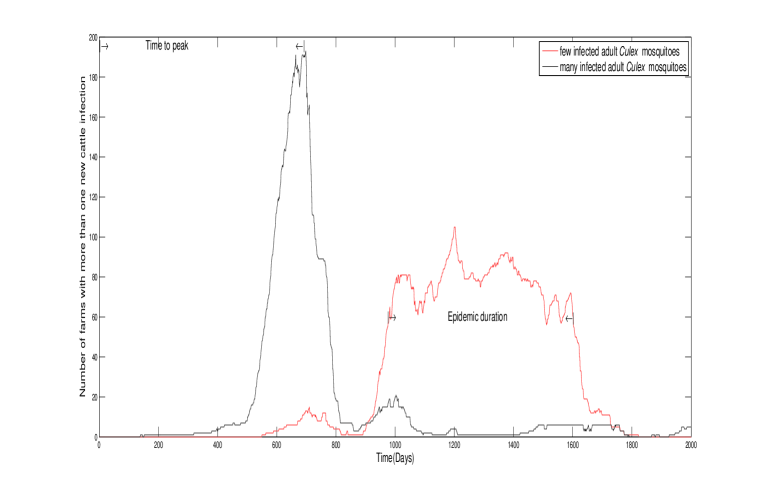
Cattle can be spreaders of virus because they are frequently bought and sold [57]. Infected cattle may infect a large number of mosquitoes via mosquito bites in a new location. In turn, the infected mosquitoes can bite a large number of susceptible cattle and transmit the virus to them. Movement bans during a RVF outbreak can restrict the further spatial spread of RVF. Therefore, very few infected cattle can infect a large number of susceptible cattle, by interacting with mosquito vectors. Early detection of infected cattle is essential. After local and regional authorities are warned and response planning initiated, such as cattle movement restrictions, culling, insecticide treatments, quarantines, and other methods to limit transmission can also be effective. These methods will be explored in future models. The cumulative number of infected cattle with few infected cattle at the beginning is larger than that with a large number of infected cattle at the beginning. The consequence caused by few initially infected cattle should also be taken seriously.

There are no human cases (integers) in the simulations regardless of initial starting conditions because of the small constant human population in each node of the study region. In high population areas, there can be a large number of human cases. Humans are often exposed to fewer mosquitoes than cattle, especially in more developed countries, which results in lower probability of being infected by mosquitoes. The probability that humans are infected by cattle is also low in this region because the model does not account for contact with the virus via animal slaughter. Hence, the number of infected humans in each farm produced by simulations is fewer than $1$. Therefore, an introduction of RVF in the study area of Texas, U.S.A. is likely to be mainly a concern for livestock farms and not an outbreak in humans as recently seen in South Africa based on the deterministic mathematical model presented by [26]. During previous outbreaks, many reported human cases proceeded with livestock cases. In the U.S.A., humans still have the potential of being infected by mosquitoes and livestock especially when many livestock cases are reported. For this reason, the dynamics of human infection during an outbreak and the factors that affect RVF virus transmission will also be studied in future models.

In conclusion, the general epidemiological trend of a smaller initial infection observed through various simulations with various initial staring locations is: $(1)$ a larger total number of infected cattle, $(2)$ a longer delay after introduction until the peak of the epidemic, and $(3)$ a more prolonged epidemic. If the infection remains small (and possibly undetected) for a longer duration, it expands geographically before the epidemic explodes involving many cattle almost simultaneously. Therefore, an established and endemic condition can generate larger epidemic disease incidence after a long period of apparent hibernation.

Table 4: Parameters in Equations (21) through (25).

Parameter	Description	Value	Source
$A_{1}$	parameter in Equation (24)	$0.15460$	[51]
$HA_{1}$	parameter in Equation (24)	$33,255.57$	[51]
$HH_{1}$	parameter in Equation (24)	$50,543.49$	[51]
$TH_{1}$	parameter in Equation (24)	$301.67$	[51]
$A$	parameter in Equation (25)	$0.25$	[44]
$HA$	parameter in Equation (25)	$28094$	[44]
$HH$	parameter in Equation (25)	$35692$	[44]
$TH$	parameter in Equation (25)	$298.6$	[44]
$b_{0}$	minimum constant fecundity rate	$0$	[44]
$Emax$	maximum daily egg laying rate	$20$	[44]
$Emean$	the mean of the daily egg laying rate	$0$	[44]
$Evar$	variance of function	$12$	[44]

Table 5: Qualitative numerical simulation results of different scenarios with respect to infected cattle. Numerical results are in Table 6 in the appendix. We define that if there is at least one cattle infected, then the farm is infected. $A$ represents the number of infected farms. $B$ represents the cumulative number of infected cattle throughout simulation. $C$ is the total number of infected cattle when the number of infected cattle farms is maximum. $D$ denotes the time to peak number of infected farms, that is, the time it takes from the first day to the day on which the largest number of infected farms appears as shown in Fig. 3. $E$ denotes epidemic duration, defined as the number of days with more than $60$ infected cattle farms. The average number of infected farms in each day is in the range of $[350,400)$, the average cumulative number of infected cattle during simulation is within the range $[350\times 10^{3},380\times 10^{3})$, and the average time to peak is within $[1000,1200)$.

			Initial	source	of	infection
Farm size	Initial infection size	Outcome characteristics	Aedes eggs	Aedes adult	Culex adult	Cattle
Small	Few ($1$)	$A$	average	small	very small	very small
		$B$	very large	very large	large	average
		$C$	very large	very large	average	very small
		$D$	very long	very long	long	medium
		$E$	medium	long	very long	short
	Many ($\gg 1$)	$A$	very small	large	very large	average
		$B$	average	small	very small	small
		$C$	very small	small	average	very small
		$D$	short	short	short	short
		$E$	short	very short	very short	very short
Large	Few ($1$)	$A$	very small	very small	very small	small
		$B$	very large	large	average	very large
		$C$	very small	small	very small	average
		$D$	long	long	short	very long
		$E$	very long	medium	short	long
	Many ($\gg 1$)	$A$	very large	very large	very large	very small
		$B$	very small	small	small	large
		$C$	average	large	average	small
		$D$	short	very short	very short	long
		$E$	very short	short	short	medium

Appendix

The quantitative simulation results of different scenarios is shown in Table 6.

Table 6: Quantitative simulation results of different scenarios. We define that if there is at least one cattle infected, then the farm is infected. The number of infected farms is represented by $A$ and the cumulative number of infected cattle throughout simulation is represented by $B$. The total number of infected cattle when the number of infected cattle farms is maximum ($C$). The time to peak number of infected farms ($D$) means the time it takes from the first day to the day on which the largest number of infected farms appears. Epidemic duration ($E$) means the number of days with more than $60$ infected cattle farms. The peak number of farms with more than one infected human is represented by $F$ and the peak number of infected humans in a single farm in one day is represented by $G$. The total number of farms is $3526$ and the total number of cattle in all farms is $303240$.

			Initial	source	of	infection
Farm size	Size of initial infection	Outcome characteristics	Aedes eggs	Adult Aedes	Adult Culex	Cattle
Small	few	$A$	$359$	$319$	$267$	$183$
		$B$	$410\times 10^{3}$	$411\times 10^{3}$	$397\times 10^{3}$	$374\times 10^{3}$
		$C$	$16288$	$6369$	$4230$	$2557$
		$D$	$1596$	$1382$	$1205$	$1012$
		$E$	$444$	$471$	$592$	$291$
		$F$	$0$	$0$	$0$	$0$
		$G$	$0$	$0$	$0$	$0$
	many	$A$	$224$	$437$	$610$	$388$
		$B$	$364\times 10^{3}$	$335\times 10^{3}$	$313\times 10^{3}$	$343\times 10^{3}$
		$C$	$1772$	$3125$	$4433$	$2773$
		$D$	$701$	$701$	$700$	$701$
		$E$	$278$	$181$	$217$	$227$
		$F$	$0$	$0$	$0$	$0$
		$G$	$0$	$0$	$0$	$0$
Large	few	$A$	$293$	$197$	$296$	$342$
		$B$	$407\times 10^{3}$	$382\times 10^{3}$	$354\times 10^{3}$	$413\times 10^{3}$
		$C$	$2907$	$3878$	$2459$	$4411$
		$D$	$1205$	$1204$	$711$	$1382$
		$E$	$557$	$443$	$278$	$467$
		$F$	$0$	$0$	$0$	$0$
		$G$	$0$	$0$	$0$	$0$
	many	$A$	$631$	$732$	$745$	$208$
		$B$	$315\times 10^{3}$	$321\times 10^{3}$	$332\times 10^{3}$	$385\times 10^{3}$
		$C$	$4251$	$4689$	$4428$	$3778$
		$D$	$700$	$655$	$608$	$1204$
		$E$	$226$	$260$	$276$	$449$
		$F$	$0$	$0$	$0$	$0$
		$G$	$0$	$0$	$0$	$0$

The outcome characteristics are classified into the following ranges.
very small ($0<A<300$ or $0<B<320\times 10^{3}$ or $0<C<3000$),
small ($300\leqslant A<350$ or $320\times 10^{3}\leqslant B<350\times 10^{3}$ or $3000\leqslant C<4000$),
average ($350\leqslant A<400$ or $350\times 10^{3}\leqslant B<380\times 10^{3}$ or $4000\leqslant C<4500$),
large ($400\leqslant A<600$ or $380\times 10^{3}\leqslant B<400\times 10^{3}$ or $4500\leqslant C<6000$),
very large ($A\geqslant 600$ or $B\geqslant 400\times 10^{3}$ or $C\geqslant 6000$),
very short or really large $(0<D<700$ or $0<E<250)$,
short $(700\leqslant D<1000$ or $250\leqslant E<300)$,
medium $(1000\leqslant D<1200$ or $300\leqslant E<450)$,
long $(1200\leqslant D<1300$ or $450\leqslant E<500)$,
very long $(D\geqslant 1300$ or $E\geqslant 500)$.

References

- 1. Daubney R, Hudson JR, Garnham PC (1931) Enzootic hepatitis or Rift Valley fever. an undescribed virus disease of sheep, cattle and man from East Africa. Journal of Pathology and Bacteriology 34: 545–579.
- 2. Favier C, Chalvet-Monfray K, Sabatier P, Lancelot R, Fontenille D, et al. (2006) Rift Valley fever in West Africa: the role of space in endemicity. Tropical Medicine & International Health 11: 1878–1888.
- 3. Martin V, Chevalier V, Ceccato P, Anyamba A, Simone LD, et al. (2008) The impact of climate change on the epidemiology and control of Rift Valley fever. Revue scientifique et technique (International Office of Epizootics) 27: 413-426.
- 4. Chevalier V, Pépin M, Plée L, Lancelot R (2010) Rift Valley fever–a threat for Europe? Eurosurveillance 15: 19506-19517.
- 5. Linthicum KJ, Davies FG, Kairo A, Bailey CL (1985) Rift Valley fever virus (family Bunyaviridae, genus Phlebovirus). isolations from Diptera collected during an inter-epizootic period in Kenya. The Journal of Hygiene 95: 197-209.
- 6. Linthicum K, Anyamba A, Tucker C, Kelley P, Myers M, et al. (1999) Climate and satellite indicators to forecast Rift Valley fever epidemics in Kenya. Science 285: 397–400.
- 7. Zeller H, Fontenille D, Traore-Lamizana M, Thiongane Y, Digoutte J (1997) Enzootic activity of Rift Valley fever virus in Senega. American Journal of Tropical Medicine and Hygiene 56: 265–272.
- 8. Bajardi P, Barrat A, Natale F, Savini L, Colizza V (2011) Dynamical patterns of cattle trade movements. PloS one 6: e19869.
- 9. Sellers RF, Pedgley DE, Tucker MR (1982) Rift Valley fever, Egypt 1977: disease spread by windborne insect vectors? The Veterinary Record 110: 73-77.
- 10. Abdo-Salem S, Waret-Szkuta A, Roger F, Olive MM, Saeed K, et al. (2011) Risk assessment of the introduction of Rift Valley fever from the horn of Africa to Yemen via legal trade of small ruminants. Tropical Animal Health and Production 43: 471-480.
- 11. Davies FG (2006) Risk of a Rift Valley fever epidemic at the haj in Mecca, Saudi Arabia. Revue scientifique et technique (International Office of Epizootics) 25: 137-147.
- 12. European Food Safety Authority (EFSA) (2005). Opinion of the scientific panel on animal health and welfare (AHAW) on a request from the commission related to “the risk of a Rift Valley fever incursion and its persistence within the community.
- 13. National Institute for Communicable Diseases (2012). Interim report on the Rift Valley fever (RVF) outbreak in South Africa. http://www.nicd.ac.za/?page=rift_valley_fever_outbreak&id=94. Accessed May 23, 2012.
- 14. Jouan A, Guenno BL, Digoutte JP, Philippe B, Riou O, et al. (1988) An RVF epidemic in southern Mauritania. Ann Inst Pasteur Virol 139: 307-308.
- 15. World Health Organization. Rift Valley fever in Sudan–Update 4. http://www.who.int/csr/don/2007_11_05/. Accessed April 19, 2012.
- 16. Sissoko D, Giry C, Gabrie P, Tarantola A, Pettinelli F, et al. (2009) Rift Valley fever, Mayotte, 2007–2008. Emerging Infectious Diseases 15: 568-570.
- 17. Kilpatrick AM (2011) Globalization, land use, and the invasion of West Nile virus. Science 334: 323-327.
- 18. Ma S, Xia Y (2009) Mathematical understanding of infectious disease dynamics. World Scientific.
- 19. Métras R, Collins LM, White RG, Alonso S, Chevalier V, et al. (2011) Rift Valley fever epidemiology, surveillance, and control: what have models contributed? Vector Borne and Zoonotic Diseases 11: 761-771.
- 20. Ross R (1916) An application of the theory of probabilities to the study of a priori pathometry. part I. Proceedings of the Royal Society of London Series A 92: 204–230.
- 21. Luz PM, Struchiner CJ, Galvani AP (2010) Modeling transmission dynamics and control of vector-borne neglected tropical diseases. PLoS neglected tropical diseases 4: e761.
- 22. Gaff H, Hartley D, Leahy N (2007) An epidemiological model of Rift Valley fever. Electronic Journal of Differential Equations 2007: 1–12.
- 23. Mpeshe SC, Haario H, Tchuenche JM (2011) A mathematical model of Rift Valley fever with human host. Acta Biotheoretica 59: 231-250.
- 24. Niu T, Gaff HD, Papelis YE, Hartley DM (2012) An epidemiological model of Rift Valley fever with spatial dynamics. Computational and mathematical methods in medicine 2012.
- 25. Gao D, Cosner C, Cantrell RS, Beier JC, Ruan S (2013) Modeling the spatial spread of rift valley fever in egypt. Bulletin of mathematical biology .
- 26. Xue L, Scott H, Cohnstaedt L, Scoglio C (2012) A network-based meta-population approach to model Rift Valley fever epidemics. Journal of Theoretical Biology 306: 129-144.
- 27. Manore C, McMahon B, Fair J, Hyman JM, Brown M, et al. (2011) Disease properties, geography, and mitigation strategies in a simulation spread of rinderpest across the united states. Veterinary research 42: 55.
- 28. Keeling M, Rohani P (2008) Modeling infectious diseases in humans and animals. Princeton University Press.
- 29. Canyon DV, Hii JLK, Muller R (1999) The frequency of host biting and its effect on oviposition and survival in Aedes aegypti (Diptera : Culicidae). Bulletin of entomological research 89: 35-39.
- 30. Hayes RO, Tempelis CH, Hess AD, Reeves WC (1973) Mosquito host preference studies in Hale county, Texas. American Journal of Tropical Medicine and Hygiene 22: 270-277.
- 31. Jones CJ, Lloyd JE (1985) Mosquitos feeding on sheep in southeastern Wyoming. Journal of the American Mosquito Control Association 1: 530-532.
- 32. Magnarelli LA (1977) Host feeding patterns of Connecticut mosquitos (Diptera-Culicidae). American Journal of Tropical Medicine and Hygiene 26: 547-552.
- 33. Pratt HD, Moore CG (1993) Vector-borne disease control: mosquitoes, of public health importance and their control. U.S. Department of Health and Human Services, Atlanta, GA.
- 34. Turell MJ, Kay BH (1998) Susceptibility of selected strains of Australian mosquitoes (Diptera: Culicidae) to Rift Valley fever virus. Journal of medical entomology 35: 132-135.
- 35. Turell MJ, Faran ME, Cornet M, Bailey CL (1988) Vector competence of senegalese Aedes fowleri (Diptera: Culicidae) for Rift Valley fever virus. Journal of Medical Entomology 25: 262-266.
- 36. Turell MJ, Bailey CL (1987) Transmission studies in mosquitoes (Diptera: Culicidae) with disseminated Rift Valley fever virus infections. Journal of Medical Entomology 24: 11-18.
- 37. Wekesa JW, Yuval B, Washino RK (1997) Multiple blood feeding by Anopheles freeborni and Culex tarsalis (Diptera: Culicidae): Spatial and temporal variation. Journal of Medical Entomology 34: 219-225.
- 38. Erasmus BJ, Coetzer JAW (1981) The symptomatology and pathology of Rift Valley fever in domestic animals. Contrib Epidemiol Biostat 3: 77-82.
- 39. Bates M (1970) The natural history of mosquitoes. Peter Smith, Gloucester, MA.
- 40. Moore CG, McLean RG, Mitchell CJ, Nasci RS, Tsai TF, et al. (1993) Guidelines for arbovirus surveillance programs in the United States. Center for Disease Control and Prevention.
- 41. Radostits OM (2001) Herd healthy: food animal production medicine. Saunders, third edition.
- 42. Peters CJ, Linthicum KJ (1994) Rift Valley fever. In: Handbook of Zoonoses. Second Edition. Section B: Viral. G.B. Beran (Ed.), Boca Raton, Fl: CRC Press, Inc. pp. 125-138.
- 43. Freier JE, Rosen L (1987) Vertical transmission of dengue viruses by mosquitoes of the Aedes scutellaris group. The American Journal of Tropical Medicine and Hygiene 37: 640-647.
- 44. Gong H, Degaetano AT, Harrington LC (2010) Climate-based models for West Nile Culex mosquito vectors in the Northeastern US. International Journal of Biometeorology 55: 435-446.
- 45. Dominguez BJ (2007) Characterization of livestock herds in extensive agricultural settings in southwest Texas. Master’s thesis, Texas A&M University, U.S.A.
- 46. United States Department of Agriculture (2007). 2007 census publications. http://www.agcensus.usda.gov/Publications/2007/Full_Report/Census_by_St%ate/Texas/index.asp. Accessed April 15, 2012.
- 47. Riley S (2010) Coping without farm location data during a foot-and-mouth outbreak. Proceedings of the National Academy of Sciences of the United States of America 107: 957-958.
- 48. Otero M, Solari H (2010) Stochastic eco-epidemiological model of dengue disease transmission by Aedes aegypti mosquito. Mathematical Biosciences 223: 32–46.
- 49. Turell MJ, Wilson WC, Bennett KE (2010) Potential for North American mosquitoes (Diptera: Culicidae) to transmit Rift Valley fever virus. Journal of medical entomology 47: 884-889.
- 50. Wonham MJ, Lewis MA, Renclawowicz J, van den Driessche P (2006) Transmission assumptions generate conflicting predictions in host-vector disease models: a case study in West Nile virus. Ecology Letters 9: 706-725.
- 51. Rueda LM, Patel KJ, Axtell RC, Stinner RE (1990) Temperature-dependent development and survival rates of Culex-quinquefasciatus and Aedes-aegypti (Diptera: Culicidae). Journal of medical entomology 27: 892-898.
- 52. National Climatic Center. NOAA Satellite and Information Service. Accessed April 18, 2012.
- 53. Linacre E (1977) A simple formula for estimating evaporation rates in various climates, using temperature data alone. Agricultural Meteorology 18: 409–424.
- 54. Longini IM (1986) The generalized discrete-time epidemic model with immunity: a synthesis. Mathematical biosciences 82: 19-41.
- 55. Brauer F, Feng Z, Castillo-Chavez C (2010) Discrete epidemic models. Mathematical biosciences and engineering 7: 1-15.
- 56. Katriel G (2013) Stochastic discrete-time age-of-infection epidemic models. International Journal of Biomathematics 6: 125066.
- 57. Arino J, Jordan R, van den Driessche P (2007) Quarantine in a multi-species epidemic model with spatial dynamics. Mathematical biosciences 206: 46-60.