User-Level Sentiment Analysis Incorporating Social Networks

Abstract

We show that information about social relationships can be used to improve user-level sentiment analysis. The main motivation behind our approach is that users that are somehow “connected” may be more likely to hold similar opinions; therefore, relationship information can complement what we can extract about a user’s viewpoints from their utterances. Employing Twitter as a source for our experimental data, and working within a semi-supervised framework, we propose models that are induced either from the Twitter follower/followee network or from the network in Twitter formed by users referring to each other using “@” mentions. Our transductive learning results reveal that incorporating social-network information can indeed lead to statistically significant sentiment-classification improvements over the performance of an approach based on Support Vector Machines having access only to textual features.

1 Introduction

Sentiment analysis [16] is one of the key emerging technologies in the effort to help people navigate the huge amount of user-generated content available online. Systems that automatically determine viewpoint would enable users to make sense of the enormous body of opinions expressed on the Internet, ranging from product reviews to political positions.

We propose to improve sentiment analysis by utilizing the information about user-user relationships made evident by online social networks. We do so for two reasons. First, user-relationship information is now more easily obtainable, since user-generated content often appears in the context of social media. For example, Twitter maintains not just tweets, but also lists of followers and followees. Second, and more importantly, when a user forms a link in a network such as Twitter, they do so to create a connection. If this connection corresponds to a personal relationship, then the principle of homophily [9] — the idea that similarity and connection tend to co-occur, or “birds of a feather flock together” [11] — suggests that users that are “connected” by a mutual personal relationship may tend to hold similar opinions; indeed, one study found some evidence of homophily for both positive and negative sentiment among MySpace Friends [23]. Alternatively, the connection a user creates may correspond to approval (e.g., of a famous figure) or a desire to pay attention (e.g., to a news source), rather than necessarily a personal relationship; but such connections are still also suggestive of the possibility of a shared opinion.

Therefore, employing Twitter as the basis for our sentiment classification experiments, we incorporate user-relation information, as follows. We first utilize a model based on the follower/followee network that has dependencies not only between the opinion of a user and the opinions expressed in his/her tweets, but also between his/her opinion and those of the users that he/she follows. We also consider an @-network-based variant, in which we have dependencies between a user’s opinion and the opinions of those whom he/she mentions via an “@”-reference.

We work within a semi-supervised, user-level framework. The reason we adopt a semi-supervised approach is that the acquisition of a large quantity of relevant sentiment-labeled data can be a time-consuming and error-prone process, as discussed later in this paper. We focus on user-level rather than tweet-level (corresponding to document- or sentence-level) sentiment because the end goal for many users of opinion-mining technologies is to find out what people think; determining the sentiment expressed in individual texts is usually a subtask of or proxy for that ultimate objective. Additionally, it is plausible that there are cases where some of a user’s tweets are genuinely ambiguous (perhaps because they are very short), but his/her overall opinion can be determined by looking at his/her collection of tweets and who he/she is connected to.

Contributions First, we empirically confirm that the probability that two users share the same opinion is indeed correlated with whether they are connected in the social network.

We then show that using graphical models incorporating social-network information can lead to statistically significant improvements in user-level sentiment polarity classification with respect to an approach using only textual information.

Additionally, we perform an array of experimental comparisons that encompasses not only the variation in underlying network (follower/followee vs. @-network) mentioned above, but also variation in how the parameters of our model are learned; how the baseline SVMs are trained; and which graph we employ, i.e., is it enough for user $v_{i}$ to follow user $v_{j}$ (corresponding to attention and/or homophily), or should we require that $v_{i}$ and $v_{j}$ mutually follow each other (more in line with homophily only)? For some topics, a combination of homophily and approval/attention links performs better than homophily links alone; but in other topics, homophily-only links are best. Interestingly, we find that when the edge quality is sufficiently high, even a very small number of edges can lead to statistically significant improvements.

Paper organization §2 gives a formal characterization of our user-level sentiment categorization problem within the setting of Twitter. §3 introduces the data set we collect and presents some motivational analysis. §4 explains our proposed model and describes algorithms for parameter estimation and prediction. §5 presents our experimental results. §6 introduces related work not mentioned otherwise. §7 concludes by summarizing our work and discussing future directions.

2 Concrete Problem Setting

In this section, we frame the problem in the context of Twitter to keep things concrete, although adaptation of this framework to other social-network settings is straightforward. In brief, we address the semi-supervised topic-dependent sentiment-polarity user categorization task. In doing so, we consider four different ways in which Twitter users can be considered to be “connected”.

Our task is to classify each user’s sentiment on a specific topic into one of two polarities: “Positive” and “Negative”. “Positive” means that the user supports or likes the target topic, whereas “Negative” stands for the opposite. (As stated above, this differs from classifying each of a user’s tweets.) Given the scale of Twitter and the difficulty in acquiring labels (see §3), we work within the semi-supervised learning paradigm. That is, we assume that we are given a topic and a user graph, where a relatively small proportion of the users have already been labeled, and the task is to predict the labels of all the unlabeled users.

Our motivating intuition, that “connected” users will tend to hold similar opinions, requires us to define what “connected” means. For Twitter, there are several possibilities. These roughly correspond to whether we should consider only “personal connections”, in accordance with homophily, or “any connection”, which is more in line with the approval/attention hypothesis mentioned in the introduction. Note that focusing on personal connections presumably means working with less data.

The first possibility we consider is to deem two Twitter users to be connected if one “follows” the other. (From now on, to distinguish between the Twitter-defined “following” relationship and ordinary English usages of the word “follow”, we use “t-follow” to refer to the Twitter version.) This corresponds to the idea that users often agree with those they pay attention to. Of course, this isn’t always true: for example, 21% of US Internet users usually consult websites that hold opposing political viewpoints [20]. So, alternatively, we may instead only consider pairs of users who know each other personally. As a rough proxy for this sort of relationship information, we look at whether a user mentions another by name using the Twitter @-convention; the intuition is that a user will address those who they are having a conversation with, and thus know. Again, though, this is only a heuristic.

Another factor to take into account is whether we should require both users in a potential pair to connect with each other. Mutual connections presumably indicate stronger relationships, but attention effects may be more important than homophily effects with respect to shared sentiment.

We thus have 2 $\times$ 2 possibilities for our definition of when we decide that a connection (edge) between users exists.

• Directed t-follow graph: user $v_{i}$ t-follows $v_{j}$ ($v_{j}$ may or may not t-follow $v_{i}$ in return).

• mutualt-follow graph: user $v_{i}$ t-follows $v_{j}$ and user $v_{j}$ t-follows $v_{i}$.

• Directed @ graph: $v_{i}$ has mentioned $v_{j}$ via a tweet containing “@$v_{j}$” ($v_{j}$ may or may not @-mention $v_{i}$ in return).

• mutual@ graph: $v_{i}$ has mentioned $v_{j}$ via a tweet containing “@$v_{j}$” and vice versa.

3 Data and Initial Observations

3.1 Data Collection

Motivation We first planned to adopt the straightforward approach to creating a labeled test set, namely, manually annotating arbitrary Twitter users as to their sentiment on a topic by reading the users’ on-topic tweets. However, inter-annotator agreement was far below what we considered to be usable levels. Contributing factors included the need for familiarity with topic-specific information and cultural context to interpret individual tweets; for example, the tweet “#lakers b**tch!” was mistakenly labeled negative for the topic “Lakers” (the expletive was spelled out in full in the original).

Fortunately, this problem can be avoided to some degree by taking advantage of the fact that user metadata is often much easier to interpret. For example, with respect to the topic “Obama”, there are Twitter users with the bios “social engineer, karma dealer, & obama lover” and “I am a right wing radical-American that is anti-Sharia law, anti-muslim, pro-Israel, anti-Obama and America FIRST”, another with username “against_obama”, and so on. We thus employed the following data-acquisition procedure.

Initial pass over users Our goal was to find a large set of users whose opinions are clear, so that the gold-standard labels would be reliable. To begin the collection process, we selected as seed users a set of high-profile political figures and a set of users who seemed opposed to them (e.g., “BarackObama”, “RepRonPaul”, “against_obama”). We performed a crawl by traversing edges starting from our seed set.

Topic selection and gold-standard user labeling In the crawl just described, the set of profiles containing the corresponding keyword tended to be hugely biased towards the positive class. We therefore used the initially-gathered profiles to try to find topics with a more balanced class distribution: we computed those keywords with the highest frequencies among the words in the profiles, resulting in the topics “Obama”, “Sarah Palin”, “Glenn Beck”, “Fox News”, and “Lakers” (e.g., “Ron Paul” was not in this final set). Then we employed a very conservative strategy: we annotated each user according to their biographical information (this information was not used in our algorithms), keeping only those whose opinions we could clearly determine from their name and bio. This approach does mean that we are working with graphs in which the users have strong opinions on the target topic, but the resulting gold-standard sentiment labels will be trustworthy.

Resultant graphs Finally, we constructed the graphs for our main experiments from the users with gold-standard labels and the edges between them. Table 1 shows basic statistics across topics. “On-topic tweets” means tweets mentioning the topic by the name we assigned it (e.g., a tweet mentioning “Barack” but not “Obama” would not be included): our experiments only consider on-topic tweets.

Table 1: Statistics for our main datasets.

Topic	# users	#t-follow edges		#@ edges		# on-topic tweets
		dir.	mutual	dir.	mutual
Obama	889	7,838	2,949	2,358	302	128,373
Sarah Palin	310	1,003	264	449	60	21,571
Glenn Beck	313	486	159	148	17	12,842
Lakers	640	2,297	353	1,167	127	35.250
Fox News	231	130	32	37	5	8,479

3.2 Observations

Before proceeding, we first engage in some high-level investigation of the degree to which network structure and user labels correlate, since a major motivation for our work is the intuition that connected users tend to exhibit similar sentiment. We study the interplay between user labels and network influence via the following two kinds of statistics:

1. Probability that two users have the same label, conditioned on whether or not they are connected

2. Probability that two users are connected, conditioned on whether or not they have the same label

As stated in §2, we have four types of user-user connections to consider: t-follow and mutually-t-follow relationships, and @-mentioned and mutually-@-mentioned relationships.

t-Follow Graph	@ Graph

Figure 1: Shared sentiment conditioned on type of connection. Y-axis: probability of two users $v_{i}$ and $v_{j}$ having the same sentiment label, conditioned on relationship type. The left plot is for the t-follow graph, while the right one is for the @ graph. “random”: pairs formed by randomly choosing users. “directed”: at least one user in the pair links to the other. “mutual”: both users in the pair link to each other. Note that the very last bar (a value of 1 for “Fox News”, mutual @-graph) is based on only 5 edges (datapoints).

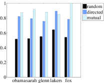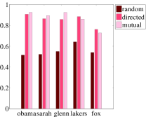
Shared sentiment conditioned on being connected Figure 1 clearly shows that the probability of two connected users sharing the same sentiment on a topic is much higher than chance. The effect is a bit more pronounced overall in the t-follow graph (red bars) than in the @-graph (blue bars): for instance, more of the bars are greater than .8. In terms of “mutual” links (mutual t-follow or @-mentions) compared with “directed” links, where the t-follow or @-mentioning need not be mutual, it is interesting to note that “mutual” corresponds to a higher probability of shared sentiment in the topics “Obama”, “Sarah Palin”, and “Glenn Beck”, while the reverse holds for “Lakers”.

t-Follow Graph	@ Graph

Figure 2: Connectedness conditioned on labels. Y-axis: probability that two users are connected, conditioned on whether or not the users have the same sentiment.

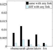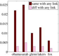
Connectedness conditioned on labels We now turn to our second statistic, which measures whether shared sentiment tends to imply connectedness. Figure 2 clearly shows that in our graphs, it is much more likely for users to be connected if they share an opinion than if they differ. The probability that same-opinion users are connected is much larger in the t-follow graph than in the @ graph. This may be a result of the fact that the @-graph is more sparse, as can be seen from Table 1.

Summary We have seen that first, user pairs in which at least one party links to the other are more likely to hold the same sentiment, and second, two users with the same sentiment are more likely to have at least one link to the other than two users with different sentiment. These points validate our intuitions that links and shared sentiment are clearly correlated, at least in our data.

4 Model Framework

In this section, we give a formal definition of the model we work with. We propose a factor-graph model for user labels. With our formulation, more-or-less standard technologies can be employed for learning and inference. We employ transductive learning algorithms in our models. The main advantage of our formulation is that it employs social-network structure to help us overcome both the paucity of textual information in short tweets and the lack of a large amount of labeled data.

4.1 Formulation

We are given a “query” topic $q$, which induces a set of users $\xmakefirstuc{v}_{q}$ who have tweeted about $q$. Our goal is to determine which users in $\xmakefirstuc{v}_{q}$ are positive towards $q$ and which are negative.

For each user $v_{i}\in\xmakefirstuc{v}_{q}$, we have the set $\mathit{tweets}_{v_{i},q}$ of $v_{i}$’s tweets about $q$, and we know which users $v_{j}\in\xmakefirstuc{v}_{q}$ t-follow or @-mention $v_{i}$ and vice versa. Recall that we are working in a semi-supervised setting where we are given sentiment labels on a relatively small subset of the users in $\xmakefirstuc{v}_{q}$. (We do not assume sentiment labels on the tweets.)

We incorporate both textual and social-network information in a single heterogeneous graph on topic $q$, where nodes can correspond to either users or tweets. Figure 3 shows an example.

Definition 1

A heterogeneous graph on topic $q$ is a graph $HG_{q}=\{\xmakefirstuc{v}_{q}\cup\{\mathit{tweets}_{v_{i},q}\>|\>v_{i}\in\xmakefirstuc{v}_{q}\},E_{q}\}$. The edge set $E_{q}$ is the union of two sets: the tweet edges $\{(v_{i},\mathit{tweets}_{v_{i},q})\>|\>v_{i}\in\xmakefirstuc{v}_{q}\}$, indicating that $v_{i}$ posted $\mathit{tweets}_{v_{i},q}$, and network-induced user-user edges.

As already mentioned in §2, we consider four types of heterogeneous graphs, characterized by the definition of when socially-induced edge $(v_{i},v_{j})$ exists in $E_{q}$: directed t-follow, mutual t-follow, directed @, and mutual @ graphs.

Tweet edges are taken to be either directed or undirected to match the type of the socially-induced edges.

Figure 3: Example directed heterogeneous graph (dependence on topic $q$ suppressed for clarity). The corresponding factor graph has factors corresponding to user-tweet dependencies (label “f”) and user-user dependencies (label “h”).

4.2 Proposed Model

Let the topic be fixed, so that we can suppress it in the notation that follows and say that we are working with heterogeneous graph $HG$ involving a set of users $V=\{v_{i}\}$. Let $y_{v_{i}}$ be the label for user $v_{i}$, and let $\mathbf{\xmakefirstuc{y}}$ be the vector of labels for all users. We make the Markov assumption that the user sentiment $y_{v_{i}}$ is influenced only by the (unknown) sentiment labels $\hat{y}_{t}$ of tweets $t\in\mathit{tweets}_{v_{i}}$ and the (probably unknown) sentiment labels of the immediate user neighbors $\mathit{Neighbors}_{v_{i}}$ of $v_{i}$. This assumption leads us to the following factor-graph-based model:

$$\begin{split}\log P(\mathbf{\xmakefirstuc{y}})=\big{(}\sum_{v_{i}\in V}\big{[}&\sum_{t\in\mathit{tweets}_{v_{i}},k,\ell}\mu_{k,\ell}f_{k,\ell}(y_{v_{i}},\hat{y}_{t})\\ &+\sum_{v_{j}\in\mathit{Neighbors}_{v_{i}},k,\ell}\lambda_{k,\ell}h_{k,\ell}(y_{v_{i}},y_{v_{j}})\big{]}\big{)}\\ -\log{Z},\end{split}$$ (1)

where the first and second inner sums correspond to user-tweet factors and user-user factors, respectively (see below for more details), and the indices $k,\ell$ range over the set of sentiment labels {0,1}. $f_{k,\ell}(\cdot,\cdot)$ and $h_{k,\ell}(\cdot,\cdot)$ are feature functions, and $\mu_{k,\ell}$ and $\lambda_{k,\ell}$ are parameters representing impact. (For instance, we might set $\mu_{0,1}$ to 0 to give no credit to cases in which user label $y_{v_{i}}$ is 0 but tweet $t$’s label $\hat{y}_{t}$ is 1.) $Z$ is the normalization factor.

User-tweet factor Feature function $f_{k,\ell}(y_{v_{i}},\hat{y}_{t})$ fires for a particular configuration, specified by the indices $k$ and $\ell$, of user and individual-tweet labels (example configuration: both are 1). After all, we expect $v_{i}$’s tweets to provide information about their opinion. Given our semi-supervised setting, we opt to give different values to the same configuration depending on whether or not user $v_{i}$ was one of the initially labeled items, the reason being that the initial labels are probably more dependable. Thus, we use $w_{{\rm labeled}}$ and $w_{{\rm unlabeled}}$ to indicate our different levels of confidence in users that were or were not initially labeled:

$$f_{k,\ell}(y_{v_{i}},\hat{y}_{t})=\left\{{\begin{array}[]{ll}{\frac{w_{{\rm labeled}}}{|\mathit{tweets}_{v_{i}}|}}&{y_{v_{i}}=k,\hat{y}_{t}=\ell,v_{i}~{}\mbox{labeled}}\\ {\frac{w_{{\rm unlabeled}}}{|\mathit{tweets}_{v_{i}}|}}&{y_{v_{i}}=k,\hat{y}_{t}=\ell,v_{i}~{}\mbox{unlabeled}}\\ {0}&\mbox{otherwise}\\ \end{array}}\right.$$ (2)

We normalize by $|\mathit{tweets}_{v_{i}}|$ because each $t\in\mathit{tweets}_{v_{i}}$ contributes to the first exponential in Eq. 1.

User-user factor Next, our observations in §3 suggest that social-network connections between users can correlate with agreement in sentiment. Hence, we define feature functions $h_{k,\ell}(y_{v_{i}},y_{v_{j}})$, which fire for a particular configuration of labels, specified by the indices $k$ and $\ell$, between neighboring users $v_{i}$ and $v_{j}$:

$$h_{k,\ell}(y_{v_{i}},y_{v_{j}})=\left\{{\begin{array}[]{ll}{\frac{w_{{\rm relation}}}{|\mathit{Neighbors}_{v_{i}}|}}&{y_{v_{i}}=k,y_{v_{j}}=\ell}\\ {0}&\mbox{otherwise}\\ \end{array}}\right.$$ (3)

Note that for a directed heterogeneous graph with edge set $E$, we define $\mathit{Neighbors}_{v_{i}}\stackrel{{\scriptstyle def}}{{=}}\{v_{j}\>|\>(v_{i},v_{j})\in E\}$, since the Twitter interface makes the tweets of t-followee $v_{j}$ visible to t-follower $v_{i}$ (and similarly for @-mentions), so we have some reason to believe that $v_{i}$ is aware of $v_{j}$’s opinions.

Implementation Note in our experiments, we empirically set the weights within the feature functions as follows: $w_{{\rm labeled}}=1.0$, $w_{{\rm unlabeled}}=0.125$, $w_{{\rm relation}}=0.6$; thus, the greatest emphasis is on tweet labels matching the label of an initially-labeled user.

4.3 Parameter Estimation and Prediction

We now address the problems of estimating the remaining free parameters and inferring user sentiment labels once the parameter values have been learned. We provide more details below, but to summarize: Inference is performed using loopy belief propagation, and for parameter estimation, we employ two approaches. The first is simple estimation from the small set of labeled data we have access to; the second applies SampleRank to the semi-supervised setting [25, 19].

4.3.1 Parameter Estimation

To avoid needing to always distinguish between $\mu_{k,\ell}$’s and $\lambda_{k,\ell}$’s, we introduce a change of notation. We write $\mathbf{\phi}$ for the vector of parameters $\mu_{k,\ell}$ and $\lambda_{k,\ell}$, and write $\Phi_{\phi}(\mathbf{\xmakefirstuc{y}})$ for the function $\log P(\mathbf{\xmakefirstuc{y}})$, given in Eq.1, induced by a particular $\mathbf{\phi}$ on a vector of user labels $\mathbf{\xmakefirstuc{y}}$. If we were in the fully supervised setting — that is, if we were given $\mathbf{\xmakefirstuc{y}}$ — then in principle all we would need to do is find the $\mathbf{\phi}$ maximizing $\Phi_{\phi}(\mathbf{\xmakefirstuc{y}})$; but recall that we are working in a semi-supervised setting. We propose the following two approaches.

Direct estimation from simple statistics (“NoLearning” for short) One way around this problem is to not learn the parameters $\mathbf{\phi}$ via optimization, but to simply use counts from the labeled subset of the data. Thus, letting $E_{\rm labeled}$ be the subset of edges in our heterogeneous graph in which both endpoints are labeled, we estimate the four user-user parameters as follows:

$$\scriptsize\lambda_{k,\ell}:=\frac{\sum_{(v_{i},v_{j})\in E_{\rm labeled}}I(y_{v_{i}}=k,y_{v_{j}}=\ell)}{\sum_{(v_{i},v_{j})\in E_{\rm labeled}}I(y_{v_{i}}=k,y_{v_{j}}=1)+I(y_{v_{i}}=k,y_{v_{j}}=0)}$$ (4)

where $I(\cdot)$ is the indicator function. Remember, though, that we do not have any labels on the (short, often hard-to-interpret) tweets. We therefore make the strong assumption that positive users only post positive (on-topic) tweets, and negative users only post negative tweets; we thus set $\mu_{k,\ell}:=1$ if $k=\ell$, 0 otherwise.

SampleRank (“Learning”) If we instead seek to learn the parameters $\mathbf{\phi}$ by maximizing $\Phi_{\phi}(\cdot)$, we need to determine how to deal with the normalization factor and how to best handle having both labeled and unlabeled data. We employ SampleRank [25], Algorithm 1:

Input: Heterogeneous graph $HG$ with labels on some of the user nodes, learning rate $\eta$

Output: Parameter values $\mathbf{\phi}$ and full label-vector $\mathbf{\xmakefirstuc{y}}$

Randomly initialize $\mathbf{\xmakefirstuc{y}}$;

Initialize $\mathbf{\phi}$ from NoLearning;

for $i:=1$ to Number of Steps do  $\mathbf{\xmakefirstuc{y}}^{\rm{new}}:={\sf Sample}(\mathbf{\xmakefirstuc{y}})$;

if (${\sf RelPerf}(\mathbf{\xmakefirstuc{y}}^{\rm{new}},\mathbf{\xmakefirstuc{y}})>0$ and ${\sf LLR}_{\mathbf{\phi}}(\mathbf{\xmakefirstuc{y}}^{\rm{new}},\mathbf{\xmakefirstuc{y}})<0$)
//performance is better but the objective function is lower
or (${\sf RelPerf}(\mathbf{\xmakefirstuc{y}}^{\rm{new}},\mathbf{\xmakefirstuc{y}})<0$ and ${\sf LLR}_{\mathbf{\phi}}(\mathbf{\xmakefirstuc{y}}^{\rm{new}},\mathbf{\xmakefirstuc{y}})>0$)
//performance is worse but the objective function is higher
then  $\mathbf{\phi}:=\mathbf{\phi}-\eta\mathbf{{\nabla_{\mathbf{\phi}}}{\sf LLR}_{\mathbf{\phi}}}(\mathbf{\xmakefirstuc{y}}^{\rm{new}},\mathbf{\xmakefirstuc{y}})$; end if convergence then  break; end if ${\sf RelPerf}(\mathbf{\xmakefirstuc{y}}^{\rm{new}},\mathbf{\xmakefirstuc{y}})>0$ then  $\mathbf{\xmakefirstuc{y}}:=\mathbf{\xmakefirstuc{y}}^{\rm{new}}$;

end end

Algorithm 1 SampleRank. In our experiments, $\eta$= .001; varying $\eta$ did not affect performance much.

In the above, ${\sf Sample}$ is the sampling function; we use the uniform distribution in our experiments . ${\sf LLR}_{\mathbf{\phi}}(\mathbf{\xmakefirstuc{y}}^{\rm{new}},\mathbf{\xmakefirstuc{y}})$ is the log-likelihood ratio for the new sample $\mathbf{\xmakefirstuc{y}}^{\rm{new}}$ and previous label set $\mathbf{\xmakefirstuc{y}}$: ${\sf LLR}_{\mathbf{\phi}}(\mathbf{\xmakefirstuc{y}}^{\rm{new}},\mathbf{\xmakefirstuc{y}})=\log\left(\frac{P(\mathbf{\xmakefirstuc{y}}^{\rm{new}})}{P(\mathbf{\xmakefirstuc{y}})}\right)=\Phi_{\phi}(\mathbf{\xmakefirstuc{y}}^{\rm{new}})-\Phi_{\phi}(\mathbf{\xmakefirstuc{y}})$ (this causes the normalization terms to cancel out). We can use all the users, labeled and unlabeled, to compute ${\sf LLR}_{\mathbf{\phi}}(\mathbf{\xmakefirstuc{y}}^{\rm{new}},\mathbf{\xmakefirstuc{y}})$, since we only need the underlying graph structure to do so (the label sets to be compared are inputs to the function).

We define the relative-performance or truth function ${\sf RelPerf}(\mathbf{\xmakefirstuc{y}}^{\rm{new}},\mathbf{\xmakefirstuc{y}})$ as the difference in performance, measured on the labeled data only, between $\mathbf{\xmakefirstuc{y}}^{\rm{new}}$ and $\mathbf{\xmakefirstuc{y}}$, where the performance ${\sf Perf}$ of a set of labels $\mathbf{\xmakefirstuc{y}}$ is ${\sf Perf}(\mathbf{\xmakefirstuc{y}})={\sf Accuracy}_{\rm labeled}(\mathbf{\xmakefirstuc{y}})+{\sf MacroF1}_{\rm labeled}(\mathbf{\xmakefirstuc{y}})$. Singh et al. [19] propose a more sophisticated approach to defining truth functions in the semi-supervised setting, but our emphasis in this paper is on showing that our model is effective even when deployed with simple learning techniques.

4.3.2 Prediction

We employ loopy belief propagation to perform inference for a given learned model, as handling the normalization factor $Z$ is still difficult. To account for the fact that SampleRank is randomized, we do learning-then-inference 5 times to get 5 predictions, and take a majority vote among the five label possibilities for each user.

5 Experiments

(a) Ground Truth	(b) Text-Only Approach	(c) Our algorithm

Figure 4: Case study: Portion of the t-follow graph for the topic “Obama”, where derived labels on users are indicated by green (positive) and red (negative), respectively. Each node is a user, and the center one is “BarackObama”. The numbers in the nodes are indices into the table below. (a): Ground truth (human annotation). (b) SVM Vote (baseline). (c) HGM-Learning in the directed t-follow graph. Filled nodes indicate cases where the indicated algorithm was right and the other algorithm was wrong; for instance, only our algorithm was correct on node 4.

Sample tweets of users classified correctly only when network information is incorporated User ID SVM Vote HGM True Tweet 1 NEG POS POS Obama is making the repubs look silly and petty. #hrc 2 NEG POS POS Is happy Obama is President Obama collectable http://tinyurl.com/c5u7jf 3 NEG POS POS I am praying that the government is able to get health care reformed this year! President Obama seems like the ONE to get it worked out!! Watching House on TV. I will be turning to watch Rachel M. next. I am hoping Pres. Obama gets his budget passed. Especially Health Care! 4 POS NEG NEG RT @TeaPartyProtest Only thing we have 2 fear is Obama himself & Pelosi & Cong & liberal news & Dems &… http://ow.ly/15M9Xv RT @GlennBeckClips: Barack Obama can no more disown ACORN than he could disown his own grandmother. #TCOT 5 POS NEG NEG RT @JosephAGallant Twitlonger: Suppose I wanted to Immigrant to Mexico? A Letter to President Obama.. http://tl.gd/1kr5rh George Bush was and acted like a war time President. Obama is on a four year power grab and photo op. #tcot 6 POS NEG NEG ObamaCare forces Americans to buy or face a fine! It is UNCONSTITUITIONAL to force us to buy obamacare. Marxist Govt. taking our Freedoms! Look up Chicago Climate Exchange,an organization formed years ago by Obama & his Marxist-Commie Cronies to form a profit off cap & trade.

In this section, we first describe our experimental procedure. We then present a case study that validates our intuitions as to how the network-structure information helps user-level sentiment classification. Finally, we analyze the performance results, and examine the effects of graph density, edge “quality”, SVM training data, and amount of unlabeled data.

5.1 Experimental Procedure

We ran each experiment 10 times. In each run, we partitioned the data for which we had ground-truth labels into a training set, consisting of 50 positive plus 50 negative randomly-chosen users whose labels are revealed to the algorithms under consideration, and an evaluation set consisting of the remaining labeled users.

One issue we have not yet addressed is our complete lack of annotations on the tweets; we need tweet labels as part of our model. We construct training data where the “positive” tweets were all (on-topic) tweets from users labeled positive, and the “negative” tweets all (on-topic) tweets from users labeled negative. (We discuss some alternative approaches later.) Different classifiers are trained for different topics.

We compare three user-classification methods, two of which were introduced in §4 and the other of which is our baseline:

• Majority-vote Baseline (SVM Vote): The user’s sentiment label is simply the majority label among their (on-topic) tweets, according to the SVM.

• Heterogeneous Graph Model with Direct estimation from simple statistics (HGM-NoLearning): We derive parameter values according to the statistics in the labeled data, and then apply loopy belief propagation to infer user sentiment labels.

• Heterogeneous Graph Model with SampleRank (HGM-Learning): We perform semi-supervised learning on the heterogeneous graph and then apply loopy belief propagation to get user-level sentiment labels.

We measure performance via both accuracy and Macro F1 on the evaluation set.

5.2 Case Study

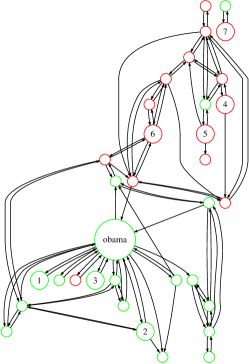
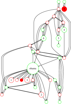
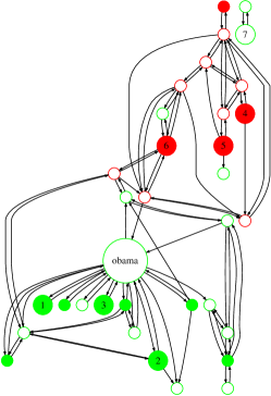
We first engage in a case study to show how our graph information can improve sentiment analysis. Figure 4 shows an example generated from our experiments. In the depicted portion (a) of the ground-truth user graph for the topic “Obama”, we see that positive (green) and negative (red) users are relatively clustered. Deriving user labels from an SVM run on text alone yields graph (b), in which we see much less clustering and a number of mistakes compared to ground truth: this is probably because tweet text is short and relatively difficult to interpret, according to our initial inspections of the data. In contrast, graph (c) shows that our text- and network-aware algorithm produces labels that are more coherently clustered and correct more often than (b).

We investigate more by looking at a specific example. The table in the lower part of Figure 4 shows a selection of tweets for users that only our algorithm classified correctly. We see that the text of these tweets is often seemingly hard (for an SVM) to classify. For example, user 1’s “Obama is making the repubs look silly and petty. #hrc” has negative words in it, although it is positive towards Obama. In these cases, the network structure may connect initially-misclassified users to users with the same sentiment, and our network-aware algorithm is able to use such relationship information to overcome the difficulties of relying on text interpretation alone.

It should be pointed out that there are cases where text alone is a better source of information. Consider user 7 in Figure 4, who resides in a two-node connected component and was correctly classified by SVM Vote but not HGM-Learning. User 7 is particularly prolific, so there is a great deal of data for the text-based SVM to work with; but the network-based method forced user 7 to share its neighbor’s label despite this preponderance of textual evidence.

5.3 Performance Analysis

Accuracy	MacroF1

Figure 5: Average Performance Analysis. Red indicates t-follow graphs, blue indicates @ graphs. For each connected pair, the left one is from NoLearning, while the right one is from Learning. A $\triangle$ marks those approaches that are significantly better than the baseline for more than 3 topics.

Accuracy
Obama	Sarah Palin	Glenn Beck	Lakers	Fox News
MacroF1
Obama	Sarah Palin	Glenn Beck	Lakers	Fox News

Figure 6: Performance Analysis in Different Topics. The x-axes are the same as in Figure 5. Bars summarize performance results for our “10-run” experiments: the bottom and top of a bar indicate the 25th and 75th percentiles, respectively. Dots indicate median results; in pairs connected by lines, the left is “NoLearning”, while the right is “Learning”. Green: SVM vote, our baseline. Red: network-based approaches applied to the t-follow graphs. Blue: results for the @ graphs. Stars ($\ast$) indicate performance that is significantly better than the baseline, according to the paired t-test.

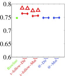
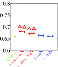
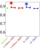
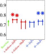
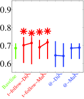
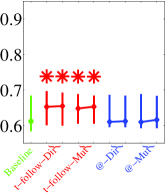
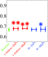
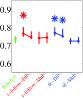
We now present the performance results for the different methods we considered. Figure 5 shows the average performance of the different methods across topics. The green dot represents the performance of the baseline, the red ones are results for t-follow graphs, and the blue ones are results for @ graphs. The presence of a $\triangle$ indicates that the corresponding approach is significantly better than the baseline for more than 3 topics.

First, our approaches all show better performance than the baseline both in Accuracy and MacroF1, though the improvement is rather small in @ graphs. This validates the effectiveness of incorporating network information.

Second, t-follow graphs (red) show better performance than @ graphs (blue). It seems that t-follow relations between people are more reliable indicators of sentiment similarity, which is consistent with our analysis of Figure 2.

Third, directed graphs work better than mutual graphs. This could either be because approval/attention links are more related to shared sentiment than any effects due to homophily, or because the directed graphs are denser than the mutual ones, as can be seen from Table 2.

Fourth, NoLearning and Learning performed quite similarly. (However, we show below that Learning can provide more robustness when more unlabeled users are added.)

Obama	Sarah Palin	Glenn Beck	Lakers	Fox News

Figure 7: Accuracy in the Largest Connected Component. We show the average accuracy in the largest connected component of the directed t-follow graph as the amount of unlabeled data increases.

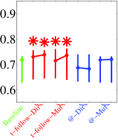
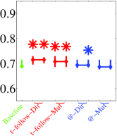
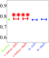
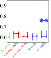
Per-topic performance: density vs. quality analysis We now look at the topics individually to gain a better understanding of what factors affect performance. Figure 6 gives the per-topic breakdown. Again, we use green, red, and blue to indicate, respectively, the SVM-vote baseline, our graph-based methods using t-follow graphs, and our graph-based methods using @ graphs. The $\ast$’s denote where our approach is significantly better than the baseline (paired t-test, .05 level). Overall, we see that for the topics “Obama”, “Sarah Palin” and “Glenn Beck”, the t-follow graph is much more effective than the @ graph in terms of providing statistically significant improvements over the baseline; but for the topics “Lakers” and “Fox”, the @ graph provides more instances of statistically significant improvements, and overall there are fewer statistically significant improvements over SVM vote. What accounts for these differences?

Table 2: Average degree statistics. Directed degree refers to out-degree.

Topic	# users	t-follow graph		@ graph
		directed	mutual	directed	mutual
Obama	889	8.8	6.6	2.7	0.7
Sarah Palin	310	3.2	1.7	1.4	0.4
Glenn Beck	313	1.6	1.0	0.5	0.1
Lakers	640	3.6	1.1	1.8	0.4
Fox News	231	0.6	0.3	0.2	0.04

Table 3: Statistics on the expanded graphs. Boldface indicates the setting used in Figure 7.

Topic	# users	# t-follow edges		#@ edges		average t-follow degree		average @ degree		total # of on-topic tweets
		directed	mutual	directed	mutual	directed	mutual	directed	mutual
Obama	307,985	60,137,108	19,204,843	8,205,166	861,394	195.3	124.7	26.6	5.6	4,873,711
Sarah Palin	121,910	14,318,290	4,278,903	3,764,747	449,568	117.5	70.2	30.9	7.4	972,537
Glenn Beck	95,847	9,684,761	3,038,396	2,862,626	357,910	101.0	63.4	29.9	7.5	687,913
Lakers	76,926	4,668,618	949,194	1,030,722	91,436	60.7	24.7	13.4	2.4	301,558
Fox News	114,530	17,197,997	5,497,221	3,889,892	462,306	150.2	96.0	34.0	8.1	1,231,519

Some initially plausible hypotheses are not consistent with our data. For instance, one might think that sparsity or having a smaller relative amount of labeled training data would affect the performance rankings. However, neither graph sparsity nor the relative or absolute amount of users in the graph explain why there are more improvements in “Glenn Beck” than “Lakers” or why “Fox News” performs relatively poorly. Table 2 shows the average degree in different topics as an approximation for sparsity. In comparison to the Glenn Beck graphs, the Lakers graphs are denser. And, Fox News has the highest proportion of labeled to unlabeled data (since it has the fewest users), but our algorithm yields relatively few improvements there.

However, the topic statistics depicted back in Figure 1 do reveal two important facts that help explain why “Lakers” and “Fox News” act differently. First, they are the two topics for which the mutual t-follow edges have the lowest probability of connecting same-label users, which explains the paucity of red $\ast$’s in those topics’ plots. Second, the reason “Lakers” and “Fox News” exhibit more statistically significant improvements for the @ graph is that, as Figure 1 again shows, they are the topics for which directed @ edges and mutual @ edges, respectively, have the highest probability among all edge types of corresponding to a shared label. Thus, we see that when the quality of the underlying graph is high, our graph-based approach can produce significant improvements even when the graph is quite sparse — for Fox News, there are only 5 mutual @ pairs. (The high performance of SVM Vote for “Lakers” makes it more difficult to make further improvements.)

Variation in SVM training We now briefly mention our experiments with two alternative training sets for the tweet-level SVM that underlies the SVM vote baseline: (a) a single set of out-of-domain tweets labeled using emoticons as distant supervision [17]; (b) the same 5 topical sets described in §5.1, except that we discarded tweets to enforce a 50/50 class balance. For (a), the statistical-significance results were roughly the same as for our main training scheme, except for “Obama”, where the SVM-vote results themselves were very poor. Presumably, a graph-based approach cannot help if it is based on extremely inaccurate information. For (b), there were some small differences in which graphs provided significant improvements; but we believe that in a semi-supervised setting, it is best to not discard parts of what little labeled data there is.

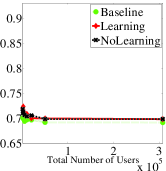
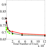
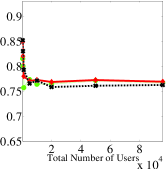
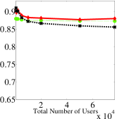
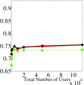
Adding more unlabeled data How much does adding more unlabeled data help? To provide some insight into this question, we consider one underlying graph type and evaluation metric — directed t-follow graph, accuracy — and plot in Figure 7 how performance is affected by increasing the number of unlabeled users. Note that what we plot is the average accuracy for the largest connected component of the labeled evaluation data, since this constitutes a more stable measure with respect to increase in overall graph size. Also, note that the way we increase the number of unlabeled users is taking them from the crawl we obtained in our initial pass over users, which contained $1,414,340$ users, $1,414,211$ user profiles, $480,435,500$ tweets, $274,644,047$ t-follow edges, and $58,387,964$ @-edges; Table 3 shows the statistics for all the expanded graphs we collected.

Figure 7 shows that HGM-Learning is generally better than the SVM Vote baseline and at worst does comparably. HGM-NoLearning tends to degrade more than HGM-Learning, suggesting that learning-based parameter estimation is effective at adjusting for graphs with more unlabeled data. Edge density does not explain the relatively larger improvements in “Lakers” and “Fox News” because those are not the densest graphs.

6 Related work

Recently, there has been some work on sentiment analysis on Twitter, focusing on the tweet level [10, 13, 3, 4, 8]. Of deployed twitter-sentiment websites (e.g., www.tweetfeel.com, www.tweetsentiments.com, www.twitrratr.com), the techniques employed are generally standard tweet-level algorithms that ignore links between users.

There has been some previous work on automatically determining user-level opinion or ideology [2, 24, 27, 12, 7], generally looking at information just in the text that the users generate.

A number of different graphs have been exploited in document- or sentence-level sentiment analysis [2, 14, 1, 15, 12, 21, 26, 22, 8], including in a semi-supervised setting [5, 6, 18]. Our use of @-mentions is similar to previous sentiment-analysis work using the network of references that one speaker makes to another [24].

7 Conclusions and future work

We demonstrated that user-level sentiment analysis can be significantly improved by incorporating link information from a social network. These links can correspond to attention, such as when a Twitter user wants to pay attention to another’s status updates, or homophily, where people who know each other are connected. Choice of follower/followee network vs @ network and directed vs. mutual connections represent different aspects of the homophily vs attention alternatives. We have some slight evidence that considering both homophily and attention is superior to homophily alone, although we also observed some exceptions. Regardless, significant gains can be achieved even when the underlying graph is very sparse, as long as there is a strong correlation between user connectedness and shared sentiment.

The general idea in this paper, to explore social network structures to help sentiment analysis, represents an interesting research direction in social network mining. There are many potential future directions for this work. A straightforward task would be to build a larger labeled dataset across more general topics; also, datasets from other online social media systems with other kinds of social networks and more information on users would also be worth exploring. Looking farther ahead, different models and semi-supervised learning algorithms for exploiting network structures should be beneficial. For example, we tried some preliminary experiments with a Markov Random Field formulation, although the sparsity of the graphs may be an issue in applying such an approach. Finding which parts of the whole network are helpful with respect to prediction on a topic is another interesting direction. Finally, building a theory of why and how users correlate on different topics in different kinds of networks is an intriguing direction for future research.

Acknowledgments Portions of this work were done while the first author was interning at Microsoft Research Asia. We thank Claire Cardie, Cristian Danescu-Niculescu-Mizil, Jon Kleinberg, Myle Ott, Karthik Raman, Lu Wang, Bishan Yang, Ainur Yessenalina and the anonymous reviewers for helpful comments. This work is supported by Chinese National Key Foundation Research 60933013 and 61035004, a Google Research Grant, a grant from Microsoft, ONR YIP-N000140910911, China’s National High-tech R&D Program 2009AA01Z138, Natural Science Foundation of China 61073073, US NSF DMS-0808864 and IIS-0910664, and a Yahoo! Faculty Research and Engagement Award.

References

- Agarwal and Bhattacharyya [2005] A. Agarwal and P. Bhattacharyya. Sentiment analysis: A new approach for effective use of linguistic knowledge and exploiting similarities in a set of documents to be classified. In ICON, 2005.
- Agrawal et al. [2003] R. Agrawal, S. Rajagopalan, R. Srikant, and Y. Xu. Mining newsgroups using networks arising from social behavior. In WWW, pages 529–535, 2003.
- Barbosa and Feng [2010] L. Barbosa and J. Feng. Robust sentiment detection on twitter from biased and noisy data. In COLING, 2010.
- Davidov et al. [2010] D. Davidov, O. Tsur, and A. Rappoport. Enhanced sentiment learning using twitter hashtags and smileys. In COLING, 2010.
- Goldberg and Zhu [2006] A. B. Goldberg and J. Zhu. Seeing stars when there aren’t many stars: Graph-based semi-supervised learning for sentiment categorization. In TextGraphs: HLT/NAACL Wksp. on Graph-based Algorithms for Natural Language Processing, 2006.
- Goldberg et al. [2007] A. B. Goldberg, J. Zhu, and S. Wright. Dissimilarity in graph-based semi-supervised classification. In AISTATS, 2007.
- Gryc and Moilanen [2010] W. Gryc and K. Moilanen. Leveraging textual sentiment analysis with social network modelling: Sentiment analysis of political blogs in the 2008 U.S. presidential election. In Proceedings of the "From Text to Political Positions" Workshop, 2010.
- Jiang et al. [2011] L. Jiang, M. Yu, M. Zhou, X. Liu, and T. Zhao. Target-dependent twitter sentiment classification. In ACL, 2011.
- Lazarsfeld and Merton [1954] P. F. Lazarsfeld and R. K. Merton. Friendship as a social process: A substantive and methodological analysis. In M. Berger, T. Abel, and C. H. Page, editors, Freedom and Control in Modern Society, pages 8–66. New York: Van Nostrand, 1954.
- Li et al. [2010] G. Li, S. C. Hoi, K. Chang, and R. Jain. Micro-blogging sentiment detection by collaborative online learning. ICDM, 0:893–898, 2010.
- McPherson et al. [2001] M. McPherson, L. Smith-Lovin, and J. M. Cook. Birds of a feather: Homophily in social networks. Annual Review of Sociology, 27:415–444, 2001.
- Mullen and Malouf [2008] T. Mullen and R. Malouf. Taking sides: User classification for informal online political discourse. Internet Research, 18:177–190, 2008.
- O’Connor et al. [2010] B. O’Connor, R. Balasubramanyan, B. R. Routledge, and N. A. Smith. From tweets to polls: Linking text sentiment to public opinion time series. In ICWSM, 2010.
- Pang and Lee [2004] B. Pang and L. Lee. A sentimental education: Sentiment analysis using subjectivity summarization based on minimum cuts. In ACL, pages 271–278, 2004.
- Pang and Lee [2005] B. Pang and L. Lee. Seeing stars: Exploiting class relationships for sentiment categorization with respect to rating scales. In ACL, pages 115–124, 2005.
- Pang and Lee [2008] B. Pang and L. Lee. Opinion mining and sentiment analysis. Foundations and Trends in Information Retrieval, 2(1-2):1–135, 1 2008.
- Read [2005] J. Read. Using emoticons to reduce dependency in machine learning techniques for sentiment classification. In ACL Student Research Wksp., 2005.
- Sindhwani and Melville [2008] V. Sindhwani and P. Melville. Document-word co-regularization for semi-supervised sentiment analysis. In Proceedings of ICDM, pages 1025–1030, 2008.
- Singh et al. [2010] S. Singh, L. Yao, S. Riedel, and A. McCallum. Constraint-driven rank-based learning for information extraction. In HLT, pages 729–732, 2010.
- Smith [2011] A. Smith. The Internet and Campaign 2010. http://www.pewinternet.org/Reports/2011/The-Internet-and-Campaign-2010.aspx, 2011.
- Somasundaran et al. [2009] S. Somasundaran, G. Namata, L. Getoor, and J. Wiebe. Opinion graphs for polarity and discourse classification. In 2009 Wksp. on Graph-based Methods for Natural Language Processing, pages 66–74, 2009.
- Tanev et al. [2010] H. Tanev, B. Pouliquen, V. Zavarella, and R. Steinberger. Automatic expansion of a social network using sentiment analysis. In Data Mining for Social Network Data, volume 12 of Annals of Information Systems, pages 9–29. Springer US, 2010.
- Thelwall [2010] M. Thelwall. Emotion homophily in social network site messages. First Monday, 15(4-5), 2010.
- Thomas et al. [2006] M. Thomas, B. Pang, and L. Lee. Get out the vote: Determining support or opposition from Congressional floor-debate transcripts. In EMNLP, pages 327–335, 2006.
- Wick et al. [2009] M. Wick, K. Rohanimanesh, A. Culotta, and A. McCallum. Samplerank: Learning preferences from atomic gradients. In NIPS Wksp. on Advances in Ranking, 2009.
- Wu et al. [2009] Q. Wu, S. Tan, and X. Cheng. Graph ranking for sentiment transfer. In Proceedings of the ACL-IJCNLP 2009 Conference Short Papers, pages 317–320, 2009.
- Yu et al. [2008] B. Yu, S. Kaufmann, and D. Diermeier. Classifying party affiliation from political speech. Journal of Information Technology & Politics, 5(1):33–48, 2008.