Wind structure and luminosity variations in the WR/LBV HD 5980

Abstract

Over the past 40 years, the massive LBV/WR system HD 5980 in the Small Magellanic Cloud has undergone a long-term S Doradus type variability cycle and two brief and violent eruptions in 1993 and 1994. In this paper we analyze a collection of UV and optical spectra obtained between 1979 and 2009 and perform CMFGEN model fits to spectra of 1994, 2000, 2002 and 2009. The results are as follows: a) The long term S Dor-type variability is associated with changes of the hydrostatic radius; b) The 1994 eruption involved changes in its bolometric luminosity and wind structure; c) the emission-line strength, the wind velocity and the continuum luminosity underwent correlated variations in the sense that a decreasing V_∞ is associated with increasing emission line and continuum levels; and d) The spectrum of the third star in the system (Star C) is well-fit by a T_eff=32 K model atmosphere with SMC chemical abundances.

For all epochs, the wind of the erupting star is optically thick at the sonic point and is thus driven mainly by the continuum opacity. We speculate that the wind switches between two stable regimes driven by the “hot” (during the eruption) and the “cool” (post-eruption) iron opacity bumps as defined by Lamers & Nugis (2002) and Gräfener and Hamann (2008), and thus the wind may undergo a bi-stability jump of a different nature from that which occurs in OB-stars.

1 Introduction

Eruptive mass-loss phenomena in massive stars is emerging as an area of interest for many reasons, one of the most important of which is that the characteristics of certain supernova explosions depend critically on the progenitor’s mass. The stars classified as Luminous Blue Variables (LBV’s) appear to have the ability to remove a large fraction of their outer stellar layers through violent ejection processes long before the SN phase is reached. It is believed that these ejections, combined with the effects of the stationary stellar winds, may determine to a large extent the mass of the supernova progenitor (van Marle et al., 2007, Smith, 2008, Dwarkadas, 2011).

The LBV eruptions have been observed since the 1600’s, but the mechanisms driving the instability have not been identified. Although some scenarios have been suggested (Guzik, 2005, Owocki & van Marle, 2008, Kashi & Soker, 2010), their confirmation is difficult due to the large distances at which most of these objects lie and the fact that they are intensely observed only after they have undergone an eruptive event. Thus, their pre-eruption characteristics are poorly constrained. Furthermore, observational constraints on their fundamental parameters are often lacking.

HD 5980 is a multiple system in the Small Magellanic Cloud that has been observed spectroscopically since the 1960s. It contains an eclipsing binary system plus a third object. Four well-defined variability timescales are present: 1) a long-term ($\sim$40 years) variation (Koenigsberger et al. 2010); 2) sudden eruptive events which were observed in 1993 and 1994, each lasting less than 1 year ( Barbá et al.1995; Koenigsberger et al. 1995, Jones & Sterken, 1997); 3) orbital-phase locked variations with the 19.3-day eclipsing binary period (Breysacher, Moffat & Niemela 1982; Foellmi et al. 2008, and references therein); and 4) “microvariability” on $\sim$30 minute timescale that was observed shortly after the 1993/1994 eruptions (Sterken & Breysacher, 1997). These timescales disclose the presence of a variety of physical phenomena in the system. In particular, Koenigsberger et al. (2010) have argued that the 1993-1994 eruptions may have been caused by tidal interactions that became stronger due to a gradual increase in the stellar radius, on the $\sim$40 year timescale. Although the process responsible for the $\sim$40 year timescale is unknown, it is believed to be the same as that which occurs in S Doradus -type variables.

The three luminous objects comprising the HD 5980 system are: two emission-line stars in a close 19.3-day binary orbit (Breysacher & Perrier 1980) and a third O-type object (hereafter star C) whose photospheric absorptions remain relatively stationary on the orbital timescale of the binary (Niemela 1988; Koenigsberger et al. 2002). Following the convention introduced by Barbá et al. (1996), we label as Star A the star “in front” at orbital phase $\phi=$0.00 and Star B the one “in front” at the opposite eclipse, which occurrs at $\phi=$0.36. Star A is the unstable star of the system (Barbá et al. 1996), and whose spectral type has changed from the Wolf-Rayet subtype WN3 (in 1978-1981; Niemela 1988) to WN6 (in 1990; Koenigsberger et al. 1994) culminating in WN11/B1.5Ia⁺ during the 1994 eruptive phase (Drissen et al., 2001; Heydari-Melayari et al., 1997; Koenigsberger et al., 1998a). Star B is believed to be a WN4 star (Breysacher, Moffat & Niemela 1982; Niemela 1988). Further background on HD 5980’s observational characteristics may be found in Barbá et al. (1996, 1997), Moffat et al. (1998), Koenigsberger (2004) and Foellmi et al. (2008).

Although its triple nature implies having to deal with the problem of disentangling the spectra of three stars and the possible contribution from a wind-wind interaction region to arrive at the eruptor’s properties, HD 5980 provides considerable advantages for studying the underlying instability: 1) its distance and masses can be relatively well-constrained; 2) it is un-obscured by dust; 3) it has been widely studied spectroscopically at X-ray, UV and optical wavelengths; and 4) it was well observed during the stages prior to the 1993–1994 eruptions and intensely observed thereafter. In this paper we focus on determining the epoch-dependent properties of Star A. Section 2 is devoted to a description of the observational data; in Section 3 we empirically disentangle the wind velocities of the three stars in the system; the existence of correlations between visual magnitude, UV brightness, emission-line strength and wind speed are shown to exist in Section 4. Section 5 contains the description of the model atmosphere fits to the spectra; the results are discussed in Section 6 and the conclusions presented in Section 7.

2 Observational material

Ultraviolet spectroscopy ($\lambda\lambda$1190–2000 Å) of HD 5980 is available from the International Ultraviolet Explorer (IUE) at low and high resolutions in 1979, 1981, 1989, 1991, and 1994–1995, and at low resolution in 1978 and 1986. The properties of these spectra were analyzed by Moffat et al. (1989) and Koenigsberger et al. (1994, 1995, 1998a, 1998b), and an overview of the derived results may be found by Koenigsberger (2004). Further UV observations at high resolution were obtained using the Hubble Space Telescope Imaging Spectrograph (STIS) in 1999, 2000, 2002 and 2009. The properties of these spectra are described by Koenigsberger et al. (2000, 2001, 2010). Tables 1 and 2 list in the first three columns the identifying number for each spectrum, the date of acquisition and the corresponding orbital phase computed with the Sterken & Breysacher (1997) initial epoch and orbital period. For many of the IUE spectra of HD 5980 a visual magnitude $m_{v}$ could be derived (Koenigsberger et al. 1994) from the Fine Error Sensor (FES) counts through the FES-$m_{v}$ calibrations (Perez 1992). These are listed in column 4 of Tables 1 and 2. The FES magnitudes have a formal error of 0.07 mag.

The IUE spectra analyzed in this paper were retrieved from the MAST data base, which contains spectra that have been re-processed with the Final Calibration. We find that the difference between the flux measurements made on these spectra and on the original data products are $<$5% for spectra obtained prior to 1992, but this difference increases significantly thereafter, in some cases being as high as 15%.

Velocities of spectral features were measured using consistent criteria for all data sets. Columns 5–6 of Table 1 list the velocities of selected features that will be described in the next section. We find that the uncertainty in the speeds measured for the P Cygni absorption components is generally $\sim$100 km/s, which we adopt throughout this paper unless otherwise noted. The sources of uncertainty include the small signal-to-noise ratio of IUE spectra, the contamination by lines arising from other atomic transitions and the definition of the continuum level. In general, the new velocity measurements coincide well, within the uncertainties, with those published previously.

The continuum flux at $\lambda$1850 Å was measured on all UV spectra and is listed in columns 9 and 7 of Tables 1 and 2, respectively. The $\lambda$1850 Å spectral region was chosen to characterize the UV continuum level because it is relatively line-free in most of the HD 5980 spectra. The integrated flux of the N IV] 1486 Å and N III 1750 Å  blend was measured and the values are listed in columns 7-8 of Table 1 and 5-6 of Table 2. Both lines are clearly associated with the active state of Star A. N IV] 1486 Å was first seen in in 1986, being absent or very weak previously. The N III 1750 Å emission was first seen during the declining phase of the 1994 eruption. It appeared as a single emission line in low resolution spectra but was composed of N III 2s²2p–2s2p² and N III 2s2p²–2p³ multiplets. The flux contained in the N IV] 1486 Å and N III emission lines was measured on the low dispersion spectra by fitting one or more Gaussian functions. On high dispersion spectra, the flux was obtained through direct integration over the emission feature. The largest source of uncertainty resides in the choice of the continuum level which is frequently difficult to define due to large number of variable emission lines and, on high resolution IUE spectra, the low signal-to-noise ratio.

The formal uncertainties in the flux calibrations of IUE and STIS data are, respectively, $\sim$6% (Colina, Bohlin & Castelli 1996) and 1% (Maíz-Apellániz & Bohlin 2005). In general, the flux levels measured in high and low resolution IUE spectra differ by no more than the quoted uncertainty. However, in the subset of observations obtained in 1994, the high resolution data display significantly weaker flux levels than the contemporaneous low resolution spectra. This situation might be due to tracking problems during the long exposures. Also, the FES counts are not available during this time period. Hence, for the analysis described in the following sections, we measured the continuum flux only on low resolution IUE data for the 1994 epoch.

An optical spectrum was obtained on 2009 November 7, at phase 0.038 using the Magellan Echellette (MagE) on the Clay 6.5m (Magellan-II) telescope on Las Campanas. We used the 1” slit providing a spectral resolution of 1 Å. Thirteen echelle orders were extracted covering the wavelength region from 3130 A to 9400 Å. The signal-to-noise ratio ranges from 100 to 200 for a single 150 s exposure. The usual ThAr comparison lamp was used for wavelength calibration. The data were reduced using the special set of IRAF routines available for the reduction of MIKE spectra (mtools package; http://www.lco.cl/telescopes-information/magellan/instruments/mike/iraf-tools). Spectra of the standards Feige 110 and NGC 7293 central star observed during the same night were used to derive a sensitivity function. The individual flux calibrated echelle orders were then normalized and merged in the final spectrum.

For the modeling discussed below, four representative spectra corresponding to different observation epochs were constructed as follows:

Spectrum 1994: The low resolution IUE spectra SWP 53218 and LWP 29794 were combined with the optical spectrum obtained on the same date, 1994 December 30, at CTIO and described in Koenigsberger et al. (1998b). This combined spectrum covers the wavelength region from 1190 Å to 6900 Å. The orbital phase is 0.39, and this is the only spectrum not obtained at primary eclipse ($\phi$=0) that we analyze. During this epoch, the spectrum of Star A was dominant and, as in Koenigsberger et al. (1998b), the contribution from Star B is neglected.

Spectrum 2000: The HST/STIS spectrum obtained on 2000 April 20 at phase 0.00. This spectrum covers the spectral range 1150 to 10800 Å.

Spectrum 2002: The HST/STIS observation of 2002 April 4, obtained at phase 0.99 was combined with the FUSE spectrum P2230101 taken on 2002 July 27 at phase 0.00. The systematic long-term variations in HD 5980 were relatively small between 2002 and 2009, justifying that we combine these two spectra obtained $\sim$3 months apart.

Spectrum 2009: The HST/STIS spectrum secured on 2009 September 9 at $\phi=$ 0.99 was combined with the Magellan-II optical spectrum obtained on 2009 November 7 at phase 0.04. As in the previous case, the long-term variability is not expected to be significant. Of greater concern is the fact that the optical spectrum was obtained 0.05 in phase later than the UV spectrum. At $\phi$=0.04 the eclipse of Star B’s continuum-emitting region is partial (see light curve in Foellmi et al. 2008).

3 Disentangling the wind velocities

The terminal wind speed $V_{\infty}$ is generally derived from the saturated portion of the P Cygni absorption component; i.e., where the intensity reaches zero level, generally referred to as $V_{black}$ (Prinja et al. 1990). In the case of a binary system, the maximum extent of the saturated profile corresponds to the speed of the slower wind in the system. The faster wind also has a $V_{black}$, but the minimum intensity level lies at the continuum level of the star whose wind is slower. Thus, as shown in Georgiev & Koenigsberger (2004), the absorption profile presents a step-like appearance. We will refer to the second $V_{black}$ as $V_{plateau}$. For single Wolf-Rayet stars, it is generally found that for saturated lines $V_{black}\sim$0.70 $V_{edge}$ (Prinja et al. 1990; Eenens & Williams 1994), where $V_{edge}$ is the location where the P Cygni absorption meets the continuum level. The observation that $V_{edge}>V_{black}$ is generally attributed to an unspecified type of “turbulence” or to non-monotonicity in the wind. In the case of optically thin lines, the P Cygni absorptions do not reach the zero flux level. In this case, $V_{edge}$ provides information on the maximum wind speed attained within the particular line-forming region.

Interpreting the P Cygni absorption components in HD 5980 is difficult because 3 massive and hot stars contribute to its spectrum. Koenigsberger et al. (1998a) adopted the purely empirical approach of measuring $V_{black}$ and $V_{edge}$ in IUE spectra obtained over the years 1979–1995. They found a persistent component at $V_{black}\sim-$1740 km/s indicating the presence of a stable wind with this speed and showed that the wind speed of Star A had undergone changes from $<$500 km/s to $\sim$ 1600 km/s during and after the 1994 eruption. However, although they suspected that Star A’s wind speed had been as high as $\sim$3000 km/s in 1979, disentangling its contribution to the P Cygni absorptions from that of the other two stars proved very challenging.

The more recent data have now clarified the picture, partly because of its greatly improved quality and partly because it has been possible to obtain UV observations during orbital phase $\phi$=0.0, when Star A occults Star B. The size of the eclipsing disk of Star A is a factor of 1.5 larger than Star B at minimum brightness (Perrier et al. 2009) and significantly larger during its more active state. It is therefore valid to assume that at orbital phases $\phi\sim$0.0 Star A eclipses star B’s continuum-forming disk as well as the P Cyg absorption forming region of star B’s wind. Thus, the P Cygni absorptions at $\phi\sim$0.0 provide the wind speeds of Star A and Star C, without contamination from Star B.

3.1 Star C: the “third” object

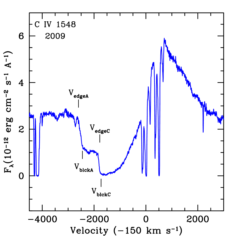
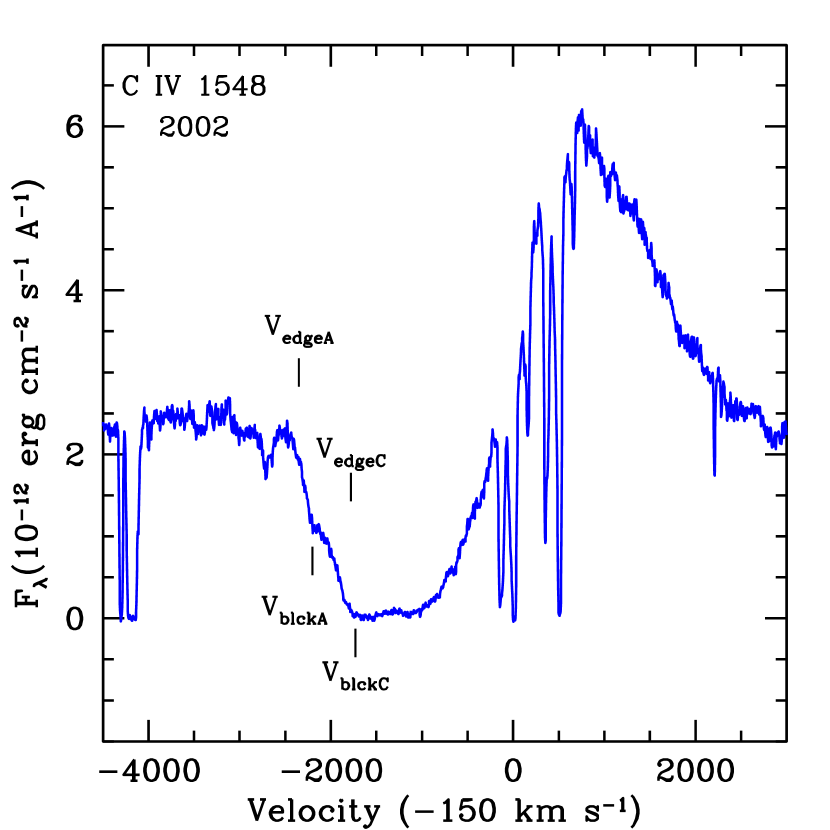
Figure 1: The C IV 1548-1550 P Cygni doublet observed in 2009 (left) and 2002 (right) on a velocity scale centered on the 1548 Å laboratory wavelength corrected for the SMC motion ($+$150 km/s).

Fig. 1 is a plot of the C IV 1548/1550 Å doublet observed in the HST/SITS spectra of 2009 (left panel) and 2002 (right panel) at orbital phase 0.99. A clear “step” is observed in the 2009 spectrum, providing two velocity values: $V_{black}$= $-$1760 km/s and $V_{plateau}$=$-$2440 km/s. The “step” is not as pronounced in the spectrum of 2002 (Fig. 1, right), but still two velocity values may be measured:$V_{black}$= $-$1780 and $V_{plateau}$=$-$2210 km/s. $V_{black}$= $-$1770$\pm$10 km/s is consistent with the persistent wind velocity measured by Koenigsberger et al. (1998a) for all epochs prior to 1996. Since only two stars are visible at $\phi$=0.99, it is now clear that this stable component is formed in Star C. These spectra also give us the wind speed of Star A in 2002 and 2009, a topic to which we shall return in Section 3.3.

3.2 Star B: the elusive companion

Of the three distinguishable objects in HD 5980, Star B is the most elusive. From the 19.3d radial velocity variations and the eclipse light curve, there is no question that Star B is a hot and massive object. However, given that Star A is such a prominent source of emission-lines, it is difficult to determine the fraction of the emission-line spectrum that may be attributed to the wind of Star B. On the other hand, during the eclipse when Star B is “in front”, the wind region of Star A where the fast portions of its P Cygni absorption components are formed is occulted. This eclipse occurs at $\phi$=0.36 and can be used to estimate Star B’s wind speed.

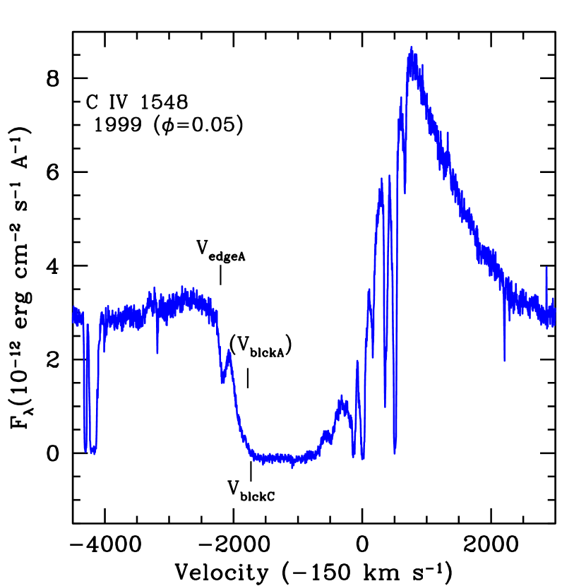
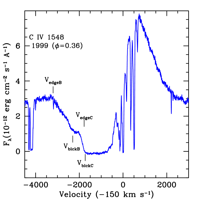
Figure 2: The C IV 1548-1550 Å  P Cygni doublet observed in 1999 at orbital phases 0.05 (left) and 0.36 (right), the latter corresponding to the eclipse when Star B is “in front”. The velocity scale is centered on the 1548 Å laboratory wavelength corrected for the SMC motion ($+$150 km/s). The large difference of 950 km/s between $V_{edgeB}$ and $V_{blckB}$ in right panel indicates a large amount of “turbulence”.

In 1999, 5 HST/STIS spectra of HD 5980 were obtained over a single orbital cycle (Koenigsberger et al. 2000), including a spectrum at $\phi$=0.36. The line-profile of C IV 1548-50 Å at this phase is shown in Fig. 2 (right) where we observe $V_{black}=-$1720 km/s, associated with Star C as discussed in the previous section. In addition, there is a short plateau that ends at $V_{plateau}$=$-$2300$\pm$100 km/s, followed by a very extended slope over which the line rises towards the continuum level extending to V_edge= 3100 km/s. We associate the $V_{plateau}$ with the terminal wind speed of Star B. The value of V_edge is consistent with the relation $V_{black}/V_{edge}\sim$0.76 typically observed for WR stars (Prinja et al. 1990). It is important to note that the eclipse at $\phi$=0.36 is not total, since Star B’s radius is smaller than that of Star A. However, the wind velocity component along the line-of-sight from the unocculted portion of Star A is rather slow and any P Cygni absorption formed in this star lies close to the rest-frame velocity. Thus, the very large value of V_edge is most likely associated with “turbulence” in the wind of Star B.

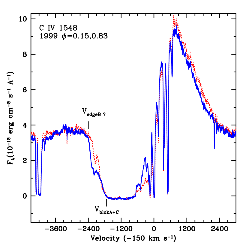
Figure 3: The C IV 1548/1550 P Cygni doublet observed in 1999 at orbital phases 0.15 (dotted line) and 0.83. These phases correspond to the largest projected orbital motion of the stars in the 19.3d binary. The “turbulet” edge velocity of $-$3100 km/s seen at $\phi$=0.36 is absent, possibly due to the wind-wind interaction region. The velocity scale is centered on the 1548 Å laboratory wavelength corrected for the SMC motion (+150 km/s).

At other orbital phases the picture is not as clear, however. Two observations at elongations were obtained as part of the same 1999 set of HST/STIS spectra mentioned above. The elongation phases observed are $\phi$=0.15 and $\phi$=0.83, when Star B is approaching the observer and receding, respectively. At $\phi$=0.15 both the $-$2300 km/s plateau and $-$3100 km/s extended absorption should be clearly visible. However, the spectrum shows only $V_{edge}\sim-$2400 km/s, as illustrated in Fig. 3. This suggests that the “turbulent” component is suppressed in the regions that are viewed expanding along-the-line of sight to the observer at $\phi$=0.15. This may be a consequence of the presence of the wind-wind interaction region, an issue that will be addressed in a forthcoming paper. For the present investigation, it suffices to keep in mind that Star B’s wind velocity is V${}_{B}\sim$ 2300 km/s and that its contribution to the system’s spectrum is important anly when it is “in front” of Star A.

3.3 Star A: the eruptor

In Fig. 2 (left) we illustrate the spectrum obtained in 1999 at $\phi=$0.05. This phase is close to primary eclipse, and Star A is between us and Star B. Here there is no plateau in the absorption line-profile indicating that Star A’s terminal wind velocity is similar to that of Star C and both stars contribute to $V_{black}$=$-$1720 km/s. In Section 3.1 we determined the wind speed of Star A in 2002 and 2009 to be 2210 and 2440 km/s, respectively. This trend for increasing wind speeds between 1999 and 2009 is one that can be traced back to late 1994, at which time speeds $<$500 km/s were recorded (Koenigsberger et al. 1998a). This is the inverse of HD 5980’s behavior in the epochs preceding the eruption; between 1979 and 1991 wind speeds steadily declined.

In the 1979 IUE spectrum obtained at $\phi=$0.91 a plateau extending to V${}_{plateau}=-$2670 km/s is clearly present in the C IV 1550 P Cygni absorption, followed by a gradual rise reaching the continuum level at $-$3200 km/s. The other spectra obtained in 1979 also display the plateau which, for example, in the case of the $\phi=$0.48 spectrum extends to $-$2750 km/s. This is similar to the $\phi$=0.36 spectrum discussed in Section 3.2. But because none of the 1979-1980 spectra were obtained during eclipse, it is not possible a priori to determine which of the two stars is responsible for the different fast components. However, since the speed determined from spectra obtained in other epochs when Star B eclipses Star A are $\sim-$2300 km/s, we are led to conclude that the $\sim-$2700 km/s component in 1979 corresponds to the wind of Star A. A similar analysis leads to the conclusion that by 1991 Star A’s wind velocity decreased to $\sim-$2200 km/s.

The individual contribution from Star A and Star B may also be identified in other P Cygni lines such as He II 1640 and N V 1240, lines to which the contribution from Star C is negligible. The N V line displays a flat portion, analogous to $V_{black}$, but which does not reach the zero intensity level. Its extent provides the velocity of the slower wind, either that of Star A or Star B, depending on the epoch. A second plateau provides the velocity of the faster wind. The measurements of these two plateaus are listed in column 6 of Table 1.

The He II 1640 line arises from a transition between two excited states, and thus, the strength of its P Cygni absorption is weaker than that of the C IV and N V resonance transitions. Here, the simplest measurement to perform is that of V_edge. Because there is no “black” portion in the absortion, it is not clear to what extent “turbulence” contributes to the edge velocity. In addition, some of the spectra show a break in the absorption profile, similar to the plateau seen in the resonance lines, and which may be associated with the second star in the system. The measured values of V_edge and of the plateau (when visible) are listed in column 5 of Table 1. We find that these values are consistent with the velocity for Star A derived from C IV and N V. Because the contribution from Star C may be neglected in N V 1240 and He II 1640, we use these lines for the analysis that will be presented in the next section.

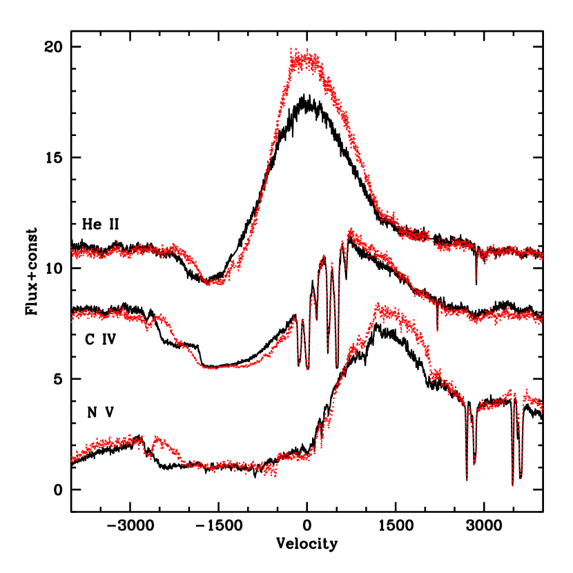
Figure 4: Montage of the N V, C IV and He II P Cygni profiles in the HST/STIS spectra obtained in 2002 (dots) and 2009. Both spectra correspond to the same orbital phase $\phi=$0.99. The most striking differences are the strength of the emission line and the extent of the absorption component. Note the “step”-like shape of the C IV absorption component in 2009 due to the contribution from Star C (-1760 km/s) and Star A (-2440 km/s). Velocity scale is centered on the laboratory wavelengths of NV1238.821, C IV 1548.187 and He II 1640.47, with a correction of $-$150 km/s to account for the relative SMC motion.

The behavior of the 3 lines is illustrated in Fig. 4 for the epochs 2002 and 2009, showing that they all display the wind velocity increase that took place between 2002 and 2009.

A summary of our estimated wind speeds for the three stars at different epochs is given in Table 3. These speeds, as those of Table 1, are corrected for the systematic velocity of the SMC ($+$150 km/s) but do not include a correction for orbital motion. It is important to note that, except for the 1979-1980 epochs, the He II 1640 values of $V_{edge}$ are systematically smaller than the values derived from C IV which are listed in Table 3. It is no clear whether this is caused by the presence of additional emission lines that “fill in” the absorption near its edge or whether this is a consequence of the excitation structure in the wind.

4 Empirical correlations

We have previously shown (Koenigsberger et al. 2010) that the emitted flux in the UV and optical lines increased during the pre-eruption epochs and decreased after $\sim$1999. Changes in the continuum flux levels have also occurred. Here we show the existence of 2 correlations and their corollaries:

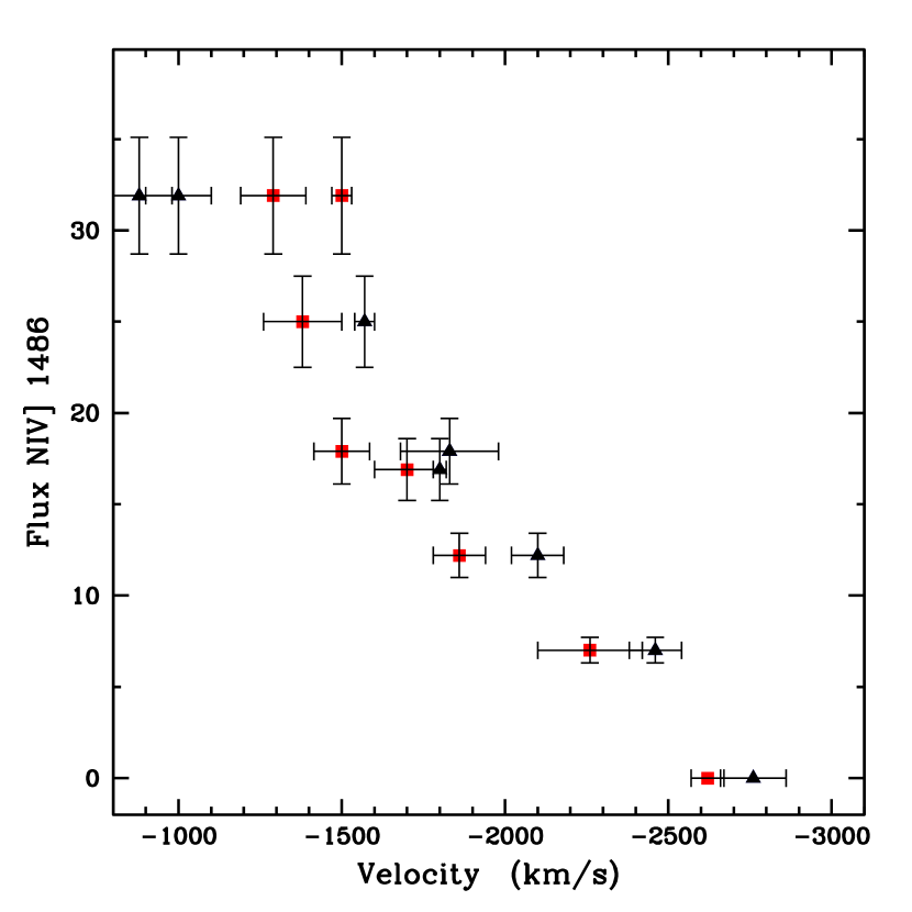
Figure 5: Line strength vs. wind velocity correlation. The N IV] 1486 Å  emission-line flux plotted against the wind velocity derived from P Cygni absorption profiles. Only data from spectra obtained around $\phi=$0.00 are plotted. Squares correpond to $V_{edge}$ of He II 1640 Å  and triangles correspond tothe saturation portion of N V 1238. Error bars in velocity correspond to estimated uncertainties in each individual measurement while the flux uncertainty is estimated at 10%.

Line strength vs. wind velocity: A decrease in the wind velocity is accompanied by an increase in the strength of the emission lines; i.e., $F_{lines}\sim V_{wind}^{-1}$. Fig. 5 shows the flux contained in the NIV] 1468 emission line plotted against the P Cygni absorption-line velocity of He II 1640 Å and N V 1240 Å. Only data from spectra obtained around $\phi=$0.00 are plotted, so the velocity clearly corresponds to that of Star A.

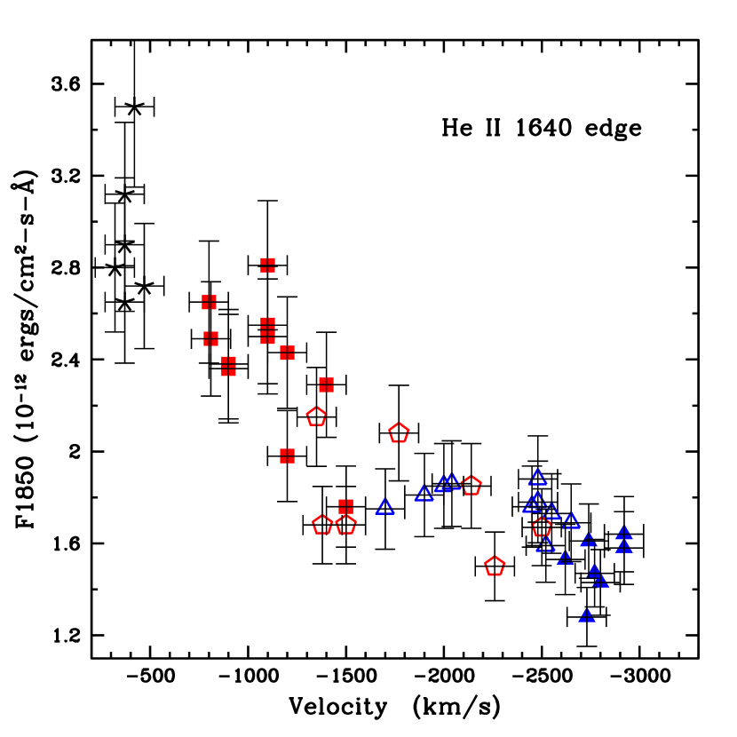
Figure 6: Continuum intensity vs. wind velocity correlation. The UV continuum flux level, F₁₈₅₀, plotted against the wind velocity derived from $V_{edge}$ of He II 1640. Symbols indicate: filled triangles – 1979–1981; open squares – 1986; open triangles – 1989–1991; stars – 1994; filled squares – 1995; and pentagons – 1999-2009. For 1994, we use values of F₁₈₅₀ measured on the low dispersion spectra.

Continuum intensity vs. wind velocity: A decrease in the wind velocity is accompanied by an increase in the strength of the continuum in the UV ($\lambda$1850 Å) and in the visual range; i.e., $F_{contin}\sim V_{wind}^{-1}$. This is illustrated in Fig. 6, where the UV continuum flux is plotted against the wind velocity measured from $V_{edge}$ of He II 1640 Å.

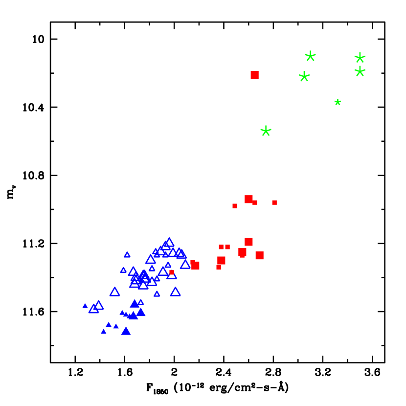
Figure 7: Visual magnitudes derived from the IUE FES counts and the continuum absolute flux values at 1850 Å. Symbols indicate: filled triangles – 1979-1981; open triangles – 1989-1991; stars – 1994; filled – 1995; Large/small symbols indicate low/high resolution spectra. The increasing trend in both wavelength regions suggests an increase in bolometric brightness.

These two correlations indicate that changes in the wind velocity are accompanied by changes in the continuum forming region as well as in the more extended line-forming regions. That is, the entire wind structure is affected. It is also important to note that the UV and the visual continuum levels increase or decrease together, as illustrated in Fig. 7. Hence, the phenomenon is not simply due to a redistribution in wavelength of the continuum energy.

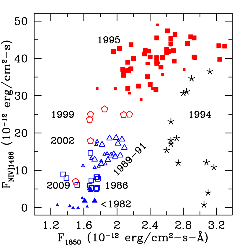
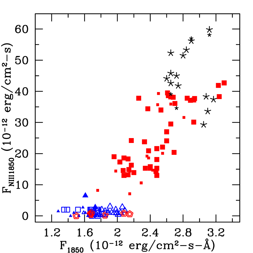
Figure 8: Absolute flux contained in the N IV]1486 Å (left) and N III 1750+1754 Å (right) emission lines plotted as a function of the absolute continuum flux at 1850 Å. The different epochs are indicated by different symbols: filled triangles – 1979–1981; open squares – 1986; open triangles – 1989–1991; stars – 1994; filled squares – 1995; and pentagons – 1999-2009. Large symbols correspond to values obtained from the IUE low resolution spectra and HST/STIS data; small symbols to high resolution IUE spectra. Uncertainties are $\sim$10% of the flux values.

A corollary of the above relations is that the continuum brightness and emission line strengths increase or decrease together; $F_{cont}\sim F_{lines}$. This is illustrated in Fig. 8, where the strengths of N IV] 1486 and N III 1750 are plotted against the flux in the continuum at 1850 Å. The different epochs of observation lie in different locations within this diagram. These results suggest that the physical phenomenon causing the changes in Star A involves an overall increase or decrease in the energy that is emitted; i.e., bolometric luminosity variations.

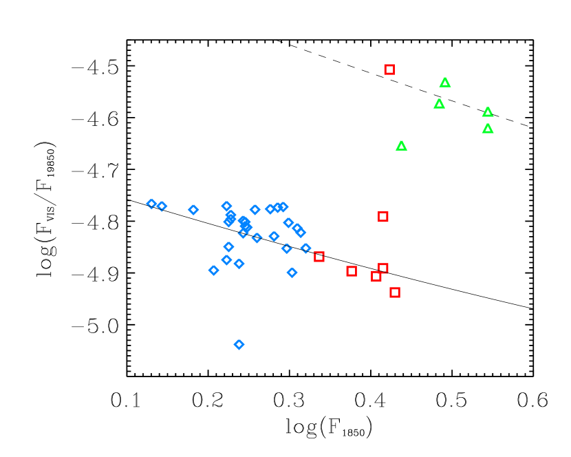
Figure 9: Ratio of the visual flux, $F_{VIS}$ converted from the IUE FES magnitudes and $F_{1850}$ from Table 2, plotted against $F_{1850}$. Small open squares - data before 1994; triangles - data of 1994; large squares - data after Jan 1995. The continuos line corresponds to the relation of $F_{VIS}$/$F_{1850}$ vs $F_{1850}$ for a black body energy distribution flux of different temperatures assuming a constant luminosity. The dashed line is the same relation but with a luminosity that is 6 times larger, implying that the 1994 eruption involved a significant change in the luminosity.

Let us momentarily assume that Star A’s continuum emits as a black body. The ratio F_vis/F₁₈₅₀ = $10^{-0.4*m(FES)}/F_{1850}$ at constant luminosity is an almost linear function of the flux at 1850 Å with F_vis/F₁₈₅₀ decreasing with the increasing temperature (continuos line on Fig. 9). The observed points in Fig. 9 are clearly separated in two groups. The points before the eruption and after 1995 lie along a curve similar to the one described by the black body, while the points obtained during the eruption are displaced from this correlation. The temperature decreased during the eruption but contrary to what might be expected, the absolute flux at 1850Å  increased, as seen in the observed F_vis/F₁₈₅₀ correlation. To account for this, the luminosity must have increased by a factor of $\sim$6 (dashed line on Fig. 9). This leads to the conclusion that the 1994 eruption involved a luminosity increase, a conclusion that is strengthened by the results of the CMFGEN modeing described in the next sections. The dispersion of the points around the black body curve during the other epochs points to some further changes in the luminosity although at a much smaller scale.

The interpretation of the line strength vs. wind velocity correlation is not straightforward. The larger V_∞ increases the transformed radius,

$$R_{t}=R_{star}\left(\frac{V_{\infty}/2500\,km/s}{\dot{M}/10^{-4}\,M_{\odot}/yr}\right)^{\frac{2}{3}}$$ (1)

(Schmutz et al. 1989) reducing the line strength. Thus, having in mind that V_∞ has been changing, one cannot directly interpret the weaker lines as a result of a lower mass loss rate. To proceed further in the interpretation of the line intensity variations it is necessary to model the spectra of Star A, which will be done in the next section.

5 CMFGEN models of Star A and Star C

As previously described, Star A undergoes two modes of large-scale variability: 1) A long term ($\sim$40 years) S Dor type variability and 2) An eruptive mode, as occurred in 1993-1994, shortly before the maximum of the S Dor cycle. The observed changes in lines and continuum fluxes that were described in Section 4 point to two separate physical states of the wind corresponding to these two modes. In order to gain further insight into the processes which drive the variability, we modeled the spectra obtained in 1994, 2000, 2002 and 2009 which are described in Section 2. These spectra correspond to times when the emission from Star A dominates over Star B’s emission. However, Star C is always present in the observations, so a model for this star was also constructed in order to adequately compare the models with the data. All comparisons are made against the sum of the fluxes from the Star A and Star C models.

We modeled the spectrum of Star A using a new version of CMFGEN code. In this version the spectrum forming region of the star is modeled as a hydrostatic photosphere and a wind attached to it. The wind is described with the usual $\beta$ law. The photosphere is specified with its gravity ($\log g$) and temperature T₁₀ at the Rosseland optical depth $\tau_{Ross}$ = 10. This large value of $\tau_{Ross}$ is chosen so that models with different mass loss rates are comparable. The density of the photosphere is calculated to satisfy the equation

$$\bigtriangledown P=-\rho(g_{grav}-g_{rad})$$ (2)

where g_grav is the specified gravitational acceleration and g_rad is the calculated acceleration due to the radiation pressure. The solution defines the density as a function of the radius. This defined density and the adopted $\dot{M}$ together with the equation of continuity defines the velocity as function of the radius. The velocity increases with decreasing density and it is connected to the wind velocity at a prescribed point which we choose to be 10 km/s. Once the velocity and density structures are specified, the radiation transport equation is solved consistently with the equations of statistical equilibrium and the energy balance as described in Hillier and Miller (1998). Several iterations of this procedure are performed until the density structure is consistent with the radiation force and the temperature distribution. The reference point at $\tau_{Ross}$ = 10 is usually situated at V(r) $\sim$ 5 km/s, below the connection point so the model parameters T₁₀ and $\log g$ apply to the underlying photosphere rather than the wind itself.

The model of the star is specified by several parameters which can be combined into two groups. In the first group, there is the chemical composition, the atomic data and the stellar mass. For the analysis of HD 5980, the values of these parameters are fixed for all epochs. The second group includes the stellar luminosity, the gravity acceleration, the temperature, the terminal velocity and the mass loss rate. For Star C, only one model fit was performed and we assume that all its derived parameters remain constant over time. For Star A, model fits were performed for each of the four spectra described in Section 2.

5.1 Star C model

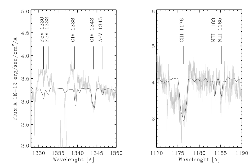
Figure 10: Fragments of 2002 HST/STIS and FUSE spectra (grey line) compared with the Star C model (black line). The model spectrum is shifted to the level of the observed spectrum which is a sum of Star A and Star C fluxes.

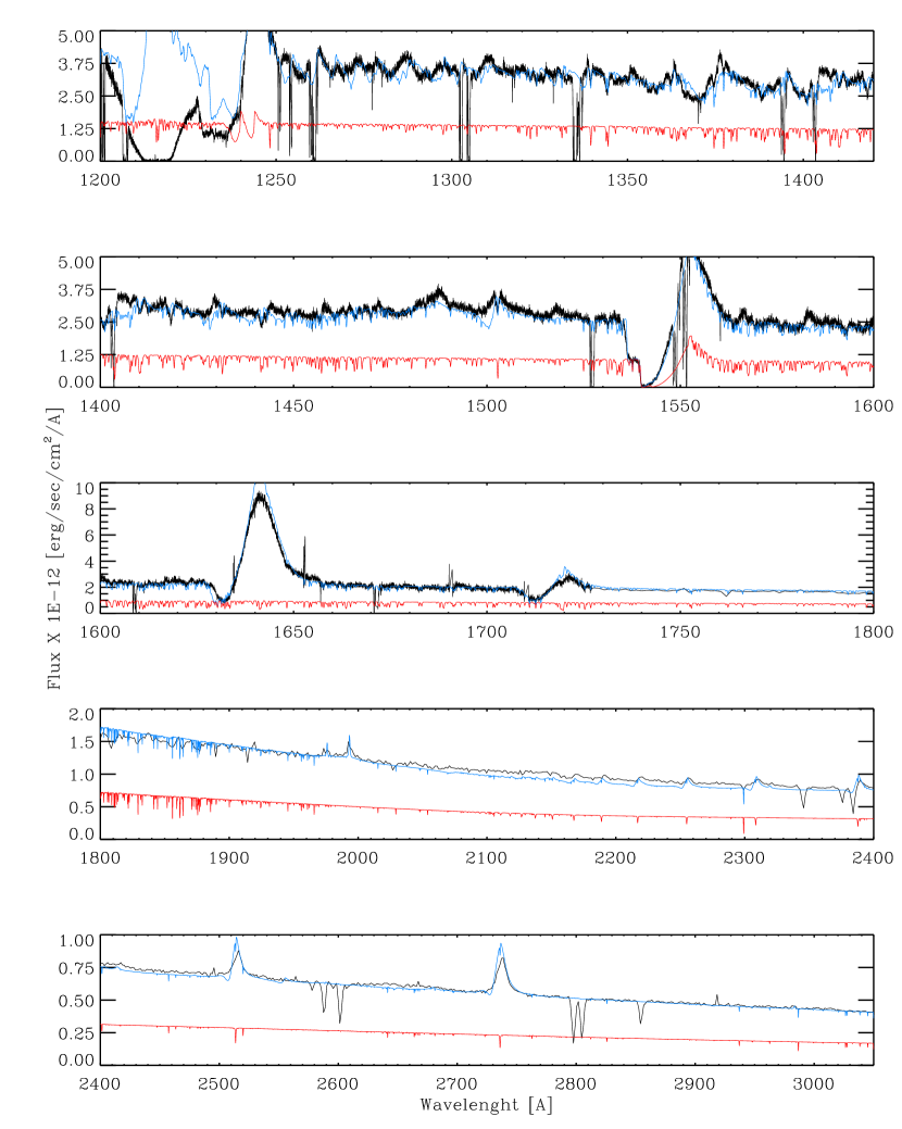
Figure 11: Comparison between the HST/STIS spectrum obtained in September 2009 (black) and the sum of the current best model for star A at this epoch and star C model. The red line represents the computed spectrum of star C alone. Notice the coincidence of the star C’s continuum and the step in the blue wind of the C IV 1548/50 Å P Cyg absorption.

Numerous photospheric absorption lines belonging to Star C (Koenigsberger et al, 2002) are clearly present in the 2009 spectrum. They were used to construct a model for this star. Hunter et al (2007) found that Si and Mg composition in B-stars in NGC 346 is $\sim$ 0.2 of the solar abundance (Table 6). Assuming this is representative for all metals heavier than O, we adopted that chemical composition. The temperature of the model was fixed by the O IV 1339-43 Å and O III 5592 Å lines. The model parameters were adjusted to attain a reasonable fit to the depth of the He I and H I optical absorption lines, clearly visible on top of the emission lines. The wind velocity was set to the observed value of $V_{black}=$ 1770 km/s and the mass loss rate was restricted to the minimal value for which the C IV 1548-50 doublet is saturated. The luminosity of Star C was fixed so that its continuum coincide with the “step” of the observed C IV 1548/50 doublet. We adopt the CNO abundances of Sk 80 (Crowther et al. 2002), with which the lines of O III 5592 Å, C III 1175 Å and C III 2297 Å and N III 1183-85 Å (Fig. 10) are adequately reproduced. The adopted parameters are shown in Column 6 of Table 6 and the spectrum is shown in Fig. 11. The model derived for Star C does not have significant emission lines in the UV-optical region other than C IV 1548-50 Å, N IV 1718 Å and N V 1239-43 Å. The comparison between the observed absorption lines and the computed spectrum suggests a rotational velocity $V_{rot}\sin{i}=$ 80 $\pm$ 15 km/s and a radial velocity $V_{r}\sim$ 60 km/s with respect to the star A + star B center of mass.

It is important to note that Schweickhardt (2000) found periodic radial velocity variations in the photospheric absorption associated with Star C, with P${}_{starC}\sim$96.5 days, and suggested that it is itself a binary system. Foellmi et al. (2008) also found RV variations in the OIII 5592.4 line consistent with Schweickhardt’s (2000) conclusion. It is thus important to keep in mind that our model for Star C corresponds to the combined spectra of two objects. A second point to keep in mind is that it remains to be determined whether this binary is gravitationally bound to the Star A $+$ Star B pair or whether it is merely a line-of-sight projection.

5.2 Star A

In this section we describe the procedure for computing the model spectrum for Star A. Because Star C is in view at all times, the computed spectrum of Star C described above was added to all models of Star A before comparison with the observed spectrum. In the cases when only the normalized observed spectrum is available we compared the observations with a model flux calculated as

$$F\left(model\right)=\frac{\left(F_{\lambda}\left(starA\right)+F_{\lambda}\left(starC\right)\right)}{\left(F_{cont}\left(starA\right)+F_{cont}\left(starC\right)\right)}$$ (3)

5.2.1 Chemical composition

We constructed a fairly complex model including most of the important atoms in several ionization stages (Table 4). The main properties of the wind were obtained for each epoch. If the observed spectrum at one epoch required an adjustment of the chemical composition, the change was made in all four epochs and the models were recalculated and the consistency checked.

The He composition was determined by the decrement of the H I and H I+He II optical lines. We fitted the lines in the spectrum obtained in 1994 and found that N(He)/N(H) = 1.0 $\pm$ 0.2 by number. This value was fixed for all 4 spectra. Due to the significant abundance of He, the mean atomic mass of the gas is larger than the Solar. In order to be able compare Star A with other objects having different He/H ratios we present the composition of all other elements by their mass fractions.

The carbon abundance was constrained mainly by C IV 5804/12Å and C III 1178 Å as observed in the 2002 FUSE spectrum. The strong C IV 1548-50 doublet is not sensitive to the abundance. The N IV 7123 Å line was used as a nitrogen abundance indicator, and consistency was checked using the UV N III, N IV and N V lines. Several iterations on all models at all epochs were made until a consistent abundance of nitrogen was obtained.

We do not observe any strong oxygen lines in the spectrum. The O IV 1338-41 Å observed in STIS spectra are formed in Star C’s wind. The weakness of these lines in Star A’s spectrum sets an upper limit to the O composition to 0.1 of the SMC value (1/50 of the solar composition). The phosphorus abundance was set to 0.05 solar. The predicted P V 1118-28 Å lines based on this value agree with the 2002 observations. S V 1502 Å line was fit with a sulfur abundance equal to 0.05 solar. The same abundance fits reasonably well S VI 933 Å as well. Aluminum abundance of 0.1 solar fits Al III 1855/63 Å doublet observed in the 1994 spectrum.

Finally, we adopted Fe/H = 0.1 (Fe/H)_⊙ by mass since this abundance reproduces well the Fe V and Fe IV lines in the spectra of the 2000, 2002 and 2009 epochs. This iron abundance is lower than the one adopted for star C (Fe/H = 0.2 (Fe/H)_⊙ ) but we did not perform a rigorous analysis of the abundances of star C and we cannot exclude that it has the same Fe/H abundance $\sim$ 0.1(Fe/H)_⊙ as of star A. Nevertheless we kept the Fe/H abundance of star C to the commonly accepted value. The lower iron abundance of star A is consistent with the result derived from a comparison of the wind-eclipse effects in HD 5980 and the Galactic WR system HD 90657 (Koenigsberger et al. 1987). For the elements Ne, Ar, Cl, Ca, Cr, Mg and Ni, we adopted a 0.1 times Solar composition similar to the iron abundance. The spectrum does not show any observable spectral features arising from these species but they are important for the line blanketing and the radiation force and were included in the model.

The composition of all other elements included in the model was also set to 0.10 of the solar value. The final chemical composition adopted for the four epochs is shown in Table 5. Note that the overall abundance for Star A is 0.1 Solar while that which was used for the Star C model is 0.2 Solar. The uncertainties in the model fits lead to uncertaintites in the chemical compositions of $\pm$0.1 dex, so that these two metalicity values are consistent, within the uncertainties.

5.2.2 Wind velocity

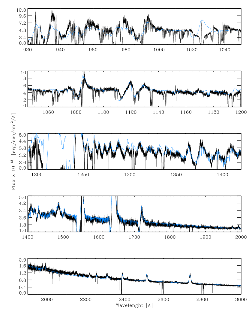
Figure 12: As if Fig. 13 but for the April 2002 epoch.

The calculated spectrum of a model is sensitive to several parameters. The first two parameters are the wind velocity law and the terminal speed, $V_{\infty}$. The Fe V and Fe VI lines in the $\lambda\lambda$1270–1450 Å region are optically thinner than the stronger lines present in the spectrum, and thus they are more sensitive to properties of the inner wind regions, particularly the velocity law. We find that a $\beta\geq$2 velocity law adequately reproduces their line-profiles. Values of $\beta<$2 produce profiles with a more “box-like” shape than observed. Thus, we set $\beta=$2. The value of V_∞ was initially chosen for each epoch from Table 3. However, we found it challenging to achieve a good fit to the P Cygni absorption components of all lines with the same value of V_∞. In general, the value of V_∞ deduced from the C IV line leads to a model in which the extent of the He II 1640 Å and P V 1118-28 Å P Cygni absorption is greater than observed (Fig. 12). The difference is $\sim$ 500 km/s. As mentioned in Section 2, the wind velocity determined from the He II 1640 P Cygni edge is systematically smaller than that derived from C IV (listed in Table 3). A slower wind velocity law (i.e. $\beta>$2) reduces this discrepancy. However, in the case of N V 1240 Å  our models require a faster $V_{\infty}$ than that derived from C IV, although the measurements of Table 2 give values that are consistent, within the uncertainties, with C IV. Increasing the value of $\beta$ does not eliminate this inconsistency in the model. Similar discrepancies are observed in some central stars of planetary nebulae (Morisset and Georgiev 2009; Herald et al. 2011; Arrieta et al. 2011). This phenomenon needs further investigation. For the purposes of this paper we used the V_∞ as derived from the C IV 1548-50 Å line and $\beta$ = 2.

5.2.3 Stellar mass and luminosity

No feature in the spectrum is clearly dependent on the gravity acceleration. This is not surprising given that the continumm forming region extends beyond the photosphere. But the mass of the star, M $\sin i$, $i$ being the orbital inclination, has been estimated from the analysis of the light curve and radial velocity curve to be between 60 and 80 M_⊙. Our modeling shows that at the observed luminosities and mass loss rates, a star with a mass smaller than 90 M_⊙ is above the Eddington limit. To keep the star stable, we assume a mass of 90M_⊙ which, within the errors, is consistent with the orbital solution and keeps the stellar photosphere below the Eddington limit. The $\log g$ was adjusted so the mass of the star is maintained the same for all epochs.

The luminosity at different epochs was determined from the continuum level of the flux calibrated UV spectra. We assume a distance to the SMC of 64 kpc which is an average of the values obtained by Hildich et al. (2005) and North et al. (2010). The reddening was determined by comparing the model and observed spectral energy distribution in the 920 Å - 11500 Å range and using the Cardelli et al. (1989) reddening law. We obtained a good fit with E(B-V)=0.065$\pm$0.005 and R = A_V/E(B-V) = 3.1 which was used for all epochs.

5.2.4 Temperature, mass-loss rate and clumping

The temperature and the mass loss rate are the most difficult parameters to determine. The change in the spectrum over the different epochs was so great that one cannot use the same diagnostic feature for the analysis for all epochs. The ever present helium lines are affected by Star B in a yet unclear way so we avoided using them. We concentrated on lines which significantly change from epoch to epoch and therefore can safely be assumed to arise in Star A. Nitrogen is present as N III, N IV and N V in different epochs and due to this variability we deduce that Nitrogen lines are formed mostly in Star A’s wind. We used the N IV 1486] line as a mass loss diagnostic and the N III 1750 Å and 4640 Å lines (when present) were used to constrain the temperature. Although we did not use the helium lines for this analysis, the fits to the He II lines are reasonably good in most of the epochs. He I lines are reasonably fit in 1994 and 2000 epochs but the models underestimate them in 2009. The profile of He I lines is also narrower for the observed V_∞. This suggests that at least part of the observed He I 5876 Å emission originates in wind-wind interaction region.

It is now well established that the winds of the massive stars are not homogeneous but rather made of clumps, although the true nature of the clumping is not known. The main effect of the clumping in the WR winds is the absence of electron scattering wings of the strong emission lines. Following the same procedure as in Hillier et al. (2003) we used the volume filling factor $f$ prescription. We adjusted $f$ until we fit the red wing of He II 4686 Å  line and then check the consistency with the other strong H I + He II lines. The observed electron scattering wings are very weak which restrict the volume filling factor to $f\leq$ 0.025. This is an upper limit to $f$. In some spectra the wings of the lines are even weaker, but smaller values for $f$ might be beyond the validity of the approximations used in the formalism. We used $f$=0.025 for all models for all epochs.

5.2.5 The individual spectral fits

Spectrum 1994: Of the four spectra, this one corresponds to the coolest temperature. N III 1750Å blend is clearly seen and we use the ratio N III 1750/N IV 1718Å  as a temperature diagnostic. The optical part of the spectrum shows N III 4640 Å line which is also well reproduced. In the low resolution IUE spectrum, the observed Fe IV lines in the 1600-1700Å  are much weaker that predicted. The mass loss rate was fixed mainly by N IV] 1486 but is consistent with the other UV emission lines. Taking into account the clumping, our derived $\dot{M}$ is in reasonable agreement with that derived in Koenigsberger et al. (1998b) for the same observed spectrum. A likely explanation for this discrepancy is that the model used in that study considered only hydrogen and helium, thus missing the important influence of the line blanketing.

Spectrum 2000: The temperature of the star is low enough to show a measurable N III 4640Å. We used that line to restrict the upper limit of the temperature. The mass loss rate was constrained by N IV] 1486 Å and further check with the Fe V UV complex. The model also reproduces well the optical He I and He II lines.

Spectrum 2002: The spectrum of this epoch does not include the optical wavelengths. We set the temperature based on the Fe VI/Fe V features observed between 1250 Å and 1400 Å and 1420 Å and 1480 Å respectively. The mass loss rate is derived from N IV] 1486 and the P V 1118-28 Å doublet.

Spectrum 2009: The temperature was limited from below by the absence of N III 4640 Å. This line is present in the previous epochs but is weak in this last spectrum. In addition we used the Fe V/Fe IV UV complex.

The uncertainties in the results obtained from the model fits are difficult to estimate due to the large number of free parameters which are not completely independent. However, the models show that changing T($\tau_{Ross}$=10) by more than $\sim$2000K causes changes in the computed spectrum that make it noticeably different from the observations. In an analogous manner, the uncertainty in the mass-loss rate can be estimated to be 30%. The uncertainty in the luminosity due to the uncertainties in the flux calibration and in the S/N of the spectra is $\lessapprox$20%. The absolute uncertainty in the parameters is much larger due to unclear correlations between them which are difficult to quantify. We minimize these errors by making our models for the different epochs consistent so the differences in the parameter values are expected to reflect real changes in the stellar physics.

5.3 Results

Table 6 summarizes the parameters derived from the models of Star A in the epochs 1994, 1999, 2002 and 2009 as well as the model of Star C. The comparison between the observations and the calculated spectra are shown in Figs. 11,  12,  13,  14 and  15.

Three different radii are listed in Table 6: 1) R₁₀, which is the radius at which the Rosseland optical depth $\tau_{Ross}$ = 10, and it is this reference radius at which the gravity acceleration is $\log{g}$ and where the temperature T₁₀, is given by the CMFGEN model; 2) R_s, which is the radius at the sonic point, were the optical depth and temperature are, respectively, $\tau_{s}$ and T_s; we define the photosphere as that region of the star with r $<$ R_s and the wind where r $>$ R_s; 3) R_2/3, which is the radius of the continuum-forming region, where $\tau_{Ross}$ = 2/3, and here T_eff = T(R${}_{2/3})$.

The most outstanding results derived from these models are:

1. The luminosity of Star A is higher during the 1994 eruptive event than at later epochs. This is consistent with the results obtained by Drissen et al. (2001) from a spectrum take on 1994 September 21. Their luminosity is even higher than our value for the spectrum obtained on 1994 December 31. The luminosity is lowest in 2000 April, and then rises slightly in 2002 remaining at the same level until 2009. Thus, we are now able to confirm that the 1994 eruption is an event which did not occur at constant luminosity.

2. Star A’s mass-loss rate is a factor of $\sim$4 larger in 1994 than at later epochs. The larger luminosity most likely plays an important role in driving the larger mass-loss rate.

3. The radius at $\tau_{Ross}$=2/3, $R_{2/3}$=124 $R_{\odot}$, is larger in 1994 than at any other epoch, and it is very much larger than $R_{s}$=21.5 $R_{\odot}$, the radius at the sonic point in 1994. The continuum-forming region is very extended. Fig. 16 shows the temperature structure of the 1994 model where one can also see that due to the larger wind density, the temperature is significantly higher throughout the wind. It is also quite remarkable that the temperature at the sonic point is $T$=10⁵ K. This high temperature is due to the fact that radiation is trapped within the extended continuum emitting region.

4. $R_{2/3}$ declines after 1994 reaching 28 R_⊙ in 2009. This value is larger than the size of the observed continuum-emitting region of Star A in 1979 (22–25 R_⊙; Perrier et al. 2009), consistent with the notion that Star A has still not recovered its minimum state of activity. The decrease in $R_{2/3}$ reflects the shrinking size of the continuum forming region as the density drops. Note, however, that $R_{s}$=19.5 $R_{\odot}$ in 2009 epoch, indicating that the continuum formation region is still rather extended.

5. The most significant change in R_s occurred in the 2000 epoch, at which time it was larger than during the other epochs. This is consistent with the long-term behavior of the optical light curve which peaked at around the 2000 epoch and with the notion that the long-term activity cycle and the brief eruptions of 1993-1994 seem to be separate phenomena (Koenigsberger et al. 2010).

6. There is a 30% variation in $\dot{M}$ between 2000 and 2002 and it remains relatively constant thereafter. Although it is tempting to suggest a declining trend, the variation lies within the uncertainties of the model results. Hence, we tentatively conclude that $\dot{M}$ is approximately constant over the timescale 2000–2009. This leads to the conclusion that the observed spectral changes during this timescale result primarily from the declining wind density, caused by the increasing wind velocity. Hence, we are now in the possibility of understanding the relation between the flux in N IV] 1486 Å and the terminal wind speed (Fig. 5). Based on the models we can conclude that the reduction of the post-eruption line intensities is caused mainly by the increase of V_∞. Assuming that V_∞/V_esc is constant (Fig. 17) one can conclude that the changes in V_∞ are caused by a decreasing radius of the star (Table 6). The relation between N IV] 1486 Å and the terminal velocity is maintained during the pre-eruption epochs and it follows the same general trend (Koenigsberger et al., 2010) but in the opposite direction. V_∞ decreases while N IV] 1486 Å increases which points to an increase in the stellar radius. This leads us to conclude that the S Dor-type $\sim$40 year variability timescale of Star A is due to variations in its radius.

The S Dor type variability of Star A is similar to that of AG Car (Groh et al. 2009) and S Dor (Lamers 1995). Excluding the 1994 eruption event, the maximum of the optical brightness in HD 5980 was attained between 1996-2000. At that time, the terminal wind velocity and the temperature were lower than in 2009, when the visual brightness was approaching its minimum. In this sense, during its long term variability, Star A behaves similarly to AG Car and S Dor. Lamers (1995) explained this variability as a pulsation of 10^-3 to 10^-2 of the stellar mass in S Dor, and Groh et al. (2009) reached the same conclusion for AG Car. Lamers (1995) suggested that the larger radius decreases the gravity acceleration and increases the scale height which leads to larger mass loss. He also suggested that the luminosity of the star should be lower during the maximum of the optical brightness due to the work the star must perform to lift the upper layers. In agreement with this prediction we detected a small difference in the luminosity in 2000 (close to maximum) and 2009 (close to minimum) epochs which add weight to the suggestion that S Dor variability of star A is caused by a pulsation. The exact physical mechanism causing the pulsation is unclear but now that we have three objects showing similar effects, the question arises as to whether this may be a common phenomenon in this class of objects.

6 The 1994 eruption and the bi-stability jump of a second kind

The results presented in Table 6 indicate that the wind structure of Star A in 1994 was significantly different from its wind structure during the other 3 epochs. This difference is best illustrated in Fig. 16 where we plot the temperature structure derived from the spectra of 1994 and 2009. The temperature is higher throughout most of the wind in 1994 than in 2009, even though the observed 1994 spectrum looks cooler. This is a consequence of the higher density in 1994 which makes the wind more optically thick.

The velocity structures are also different, in particular, the relation between the terminal wind velocity, V_∞ and the escape velocity V_esc, which is defined as

$$V_{esc}=\left(\frac{GM\left(1-\Gamma\right)}{R_{10}}\right)^{1/2}$$ (4)

where M is the stellar mass assumed to be 90 M_⊙. The ratio between gravity acceleration and the radiation pressure $\Gamma=g_{el}/g_{grav}$ takes into account only the radiation pressure caused by electron scattering (Lamers and Cassineli, 1999). We calculate V_esc using $\Gamma$ as determined by the CMFGEN model at R₁₀. Fig. 17 shows V_∞ plotted against V_esc. The values for the three post-eruption epochs (2000, 2002 and 2009) lie close to a single straight line, the slope of which is $\sim$ 2.3. The wind during the 1994 epoch is different. In this case, V_∞/V${}_{esc}~{}\sim$ 1.2. The velocities obtained by the Drissen at al. (2001) for 1994 September lie along the same relation.

The change in the V_∞/V_esc relation together with the cooler effective temperature of the 1994 spectrum are strongly suggestive of a phenomenon associated with the bi-stability jump (Lamers et al. 1995). The bi-stability jump occurs when the temperature in the inner wind decreases to a value at which the ionization fraction of Fe²⁺ increases leading to changes in the line opacities and a changes of the driving force, higher mass loss rate and reduce in V_∞/V_esc from $\sim$2.6 to 1.3 (Vink et al, 1999). This occurs at $T_{eff}\sim$21000 K.

This is remarkably similar to what we find for HD 5980. There is, however, a major difference between the cause of the bi-stability jump observed in O and B stars and the phenomenon that our models indicate is occurring in HD 5980. As was shown by Lamers and Cassinelli, (1999) and Vink et al. (1999), the mass loss rate is defined by the force below the sonic point. In the optically thin O and B star’s winds the sonic point is above the photosphere, thus the condition in it can be described by the effective temperature. On the other hand, the sonic point of the optically thick wind of HD5980 is located below the pseudo photosphere (Fig. 16). In the 1994 model, the point at which the temperature T$\sim$T${}_{eff}\sim$21000 K lies at $\sim$6 $R_{s}$ far above the sonic point. Thus, changes in the ionization structure at a distance of $\sim$6 $R_{s}$ have little effect on the overall wind structure.

In search of an alternative cause of the jump we followed the reasoning of Lamers and Nugis (2002), and Gräfener and Hamman, (2008). These authors showed that the WR winds below the sonic point are driven not by the line force but rather by the radiation pressure due to continuum opacities. We applied that idea to star A’s wind. In Table 6 we see that the optical depth of the sonic point $\tau_{s}>$ 1 for all four epochs, indicating that the wind is driven primarily by the continuum force. Lamers and Nugis (2002), and Gräfener and Hamman, (2008) showed that in order to drive a WR-type wind, the continuum opacity (sum of the true continuum opacities and the pseudo continuum of overlapping lines) has to be dominated by one of the bumps in the iron opacity. Gräfener and Hamman, (2008) showed that the required high mass loss rate is obtained only if the temperature at the sonic point is either in the 30-70kK range (“cool” bump) or around 160kK (“hot” bump). Table 6 shows that all of the post eruption models have T${}_{s}\sim$ 48–50 kK, well within the first of these temperature intervals. One can thus expect that at almost constant luminosity the mass loss rate will be almost constant, which is indeed the result from our models (Table 6). During the eruption the luminosity of the star increased. The higher luminosity heated the inner part of the wind changing the opacity contributors from those of the “cool” bump to those of the “hot” bump, thus changing the driving force and therefore the mass loss rate. Our model for 1994 December gives T_s = 100kK (Table 6). This temperature is too high for the “cool” iron opacity bump but too cool for the “hot” bump at 160kK. Gräfener and Hamman 2008) suggested that winds with T_s in the intermediate temperature range are unstable. We speculate that at the onset of the eruption T_s was high enough and the very dense wind was driven by the high temperature iron bump. As the luminosity decreased, the cooler wind became unstable and it rapidly switched back to the “cool” iron bump driving with T_s around 50 kK.

We suggest that a bi-stability jump of a second kind operates in Star A. The sudden change in the wind properties is due to a transition from the “hot” to the “cool” Fe-bump opacity regimes mechanism that was shown by Lamers & Nugis (2002) and Gräfener & Hamann (2008) to be needed to drive the winds of WR stars.

Our models show that the increased luminosity can indeed change T_s, changing the entire wind structure during the eruption. Fig. 16 shows the change in the temperature structure of the wind in the 1994 and 2009 models. In the less dense wind of 2009, the continuum forming region has moved further in and T_eff increased. The sonic point is at a similar radius but due to the overall smaller temperature gradient it is significantly cooler. In addition to the changes in the temperature, the value of $\Gamma$ changes from $\sim$ 0.75 during the eruption to $\sim$ 0.53 afterward. A similar result was found by Smith et al. (2004). These authors showed that when the star approaches the Eddington limit, the optical depth of the sonic point increases and it moves below the photosphere. The increased luminosity of star A moved it closer to the Eddington limit and the wind reacted in a similar manner. Furthermore Gräfener and Hamann (2008) found that the WN stars with SMC chemical composition require $\Gamma>$ 0.75 to maintain a high mass loss rate. In addition the Vink et al. (2011) models show a transition from O star wind to WR wind when $\Gamma$ increases above 0.7. Based on these considerations we can conclude that the wind during the eruption is governed by different forces then the wind in the post eruption epochs. We speculate that during the eruption, the high luminosity heats the inner part of the wind, driving much higher mass loss trough the “hot” iron opacity bump. After the eruption the temperature at the sonic point drops making the wind unstable. The mass loss rate drops, which causes further cooling of the sonic point until it reaches the “cool” iron bump where the wind stabilizes again and the star continues its long-term variability but with a restructured wind.

Hence, we suggest that for the dense winds such as those in HD 5980, there exists a second type of bi-stability jump than that proposed by Lamers et al. (1995). It is caused by transition between the “hot” and “cold” iron opacity bump and is correlated mainly with the stellar luminosity rather than with the effective temperature. Smith et al (2004) discussed the position of the sonic point in the typical LBVs. They showed that for the derived parameters of most of the LBVs, the sonic point is located above the photosphere and thus their winds change according to the “classical ” bi-stability jump. Here we speculate that the most luminous LBVs, such as star A, have optically thick winds with pseudo photospheres above their sonic points even on the hotter side of the S Dor instability strip. Thus their excursion to the cool branch of the strip is coused by a second kind of bi-stability jump related to the changes in their continuum opacities.

7 Conclusions

HD 5980 is a relatively nearby system in which processes involving eruptive phenomena and massive star evolution in binary systems in a low metallicity environment can be studied. In this respect, is important to gain an understanding of the phenomena that it has presented over the past few decades.

In this paper we present the results of the analysis of a collection of UV and optical spectra obtained between 1979 and 2009 and performed CMFGEN model fits to spectra of 1994, 2000, 2002 and 2009. The primary results are as follows: a) The long term S Dor-type variability is associated with changes of the hydrostatic radius. We find that the radius of the eruptor at the sonic point was largest in the year 2000 (R_s=24.3 R_⊙), coinciding with the long-term maximum in the visual light curve. The minimum value in our data set is in 2009 (R_s=19.6 R_⊙).

b) The 1994 eruption involved changes in the eruptor’s bolometric luminosity and wind structure. The luminosity was larger by at least 50% with respect to the subsequent epochs and the temperature throughout most of the wind was significantly higher. The latter is a consequence of the very large optical depth which causes photons to be trapped within this wind region. At the same time, the velocity structure was one in which the relationship between the terminal wind velocity and the escape velocity V_∞/V${}_{esc}\sim$1.2, contrary to other epochs in which this ratio was $\sim$2.3. c) the emission-line strength, the wind velocity and the continuum luminosity underwent correlated variations in the sense that a decreasing V_∞ was associated with increasing emission line and continuum levels. These correlations can be understood in the context of the increasing size of the hydrostatic stellar radius. d) The spectrum of the third star in the system (Star C) is well-fit by a T_eff=32 K model atmosphere with SMC chemical abundances. The abundances of the eruptor, Star A, show He and N enhancements, roughly consistent with the CNO cycle equilibrium values. A similar composition was obtained by Groh et al. (2009) for AG Car and Hillier et al. (2001) for $\eta$ Car.

For all epochs, the wind of the erupting star is optically thick at the sonic point and is thus driven mainly by the continuum opacity. We speculate that the wind switches between two stable regimes driven by the “hot” (during the eruption) and the “cool” (post-eruption) iron opacity bumps as defined by Lamers & Nugis (2002) and Gräfener and Hamann (2008), and thus the wind may undergo a bi-stability jump of a different nature from that which occurs in OB-stars.

8 Acknowledgements

We thank Alfredo Díaz and Ulises Amaya for computing assistance. This research was supported under UNAM/DGAPA/PAPIIT grants IN106798, IN123309 and CONACYT grants 48929 and 83016. LNG acknowledges the support from CONACyT grant 141530. RHB acknowledges partial support from ULS DIULS grant, and DJH acknowledges support from grant HST-GO-11623.01-A and HST-GO-11756.01. The HST is operated by the STSCI, under contract with AURA.

Table 1: High dispersion spectra

Spectrum	HJD	Phase	FES mag	HeII${}_{edge}\tablenotemark{2}$	NVsat	F(N IV])	F(NIII)	F(1850Å)
4277	43921.1	0.57	11.68	-2770	-2800	$<$ 1.	1.0	1.47
4345	43928.6	0.91	11.69	-2620	-2760	$<$ 1.	$<$1	1.53
4958	43981.0	0.68	11.72	-2800	-2050	$<$ 1.	$<$1	1.43
	$\cdots$	$\cdots$	$\cdots$	$\cdots$	-2790	$\cdots$	$\cdots$	$\cdots$
11175	44632.3	0.48	11.61	-2920	-2610	2.8	2.7	1.58
11190	44634.6	0.60	11.63	-2920	-2540	$<$1.3	$<$1	1.64
15072	44869.5	0.80	11.62	-2740	-2450	1.9:	$<$1	1.61
15080	44870.5	0.85	11.57	-2730	-2130	0.7:	1.5	1.28
	$\cdots$	$\cdots$	$\cdots$	$\cdots$	-2650	$\cdots$	$\cdots$	$\cdots$
37759	47867.2	0.39	11.36	-2520	-2210	11.2	1.	1.59
	$\cdots$	$\cdots$	$\cdots$	-2080	$\cdots$	$\cdots$	$\cdots$	$\cdots$
37768	47868.2	0.44	11.27	-2550	-2050	10.7	$<$1	1.62
	$\cdots$	$\cdots$	$\cdots$	-1890	$\cdots$	$\cdots$	$\cdots$	$\cdots$
37781	47870.2	0.55	11.27	-2040	-l750	11.7	$<$1	1.86
37788	47871.4	0.61	11.25	-2000	-1950	14.3	0.2	1.85
42446	48511.5	0.83	11.41	-1900	-1980	12.5	$<$1	1.86
42470	48515.6	0.05	11.35	-1700	-1800	16.9	$<$1	1.82
42694	48541.4	0.39	11.55	-2650	-2450	13.2	1.	1.73
42702	48542.4	0.44	11.50	-2480	-2340	11.1	2.	1.86
42711	48543.4	0.49	11.27	-2480	-2210	14.5	1.4	1.93
42721	48544.4	0.54	11.33	-2450	-2180	17.8	$<$1	1.95
52888	49680.5	0.51	11.37	-420	$\cdots$	7.4	18.8	3.32
53036	49697.5	0.39	$\cdots$	-370	$\cdots$	14.0:	39.1:	1.96::
53129	49706.5	0.86	$\cdots$	-470	$\cdots$	6.9:	34.6:	1.75::
53216	49716.5	0.38	$\cdots$	-370	-1680	23.9	57.0	2.55:
53226	49717.5	0.43	11.12	-370	-1730	21.9	58.1	2.55:
54064	49784.1	0.89	$\cdots$	-1100	-2010	38.8	39.3	2.50
54490	49831.0	0.32	11.96	-800	$\cdots$	43.6	35.9	2.65
	$\cdots$	$\cdots$	$\cdots$	-1900	-1660	$\cdots$	$\cdots$	$\cdots$
54671	49851.0	0.36	11.98	-810	-950:	49.0	35.7	2.49
	$\cdots$	$\cdots$	$\cdots$	-2000	-1900	$\cdots$	$\cdots$	$\cdots$
54727	49859.9	0.82	11.96	-1100	-900	37.0	31.6	2.81
	$\cdots$	$\cdots$	$\cdots$	-2400	-2300	$\cdots$	$\cdots$	$\cdots$
55315	49916.8	0.78	11.27	-1100	-800:	35.9	20.1	2.55
	$\cdots$	$\cdots$	$\cdots$	-2530	-2150	$\cdots$	$\cdots$	$\cdots$
55380	49928.8	0.40	11.34	-900	-1130	38.2	19.2	2.36
	$\cdots$	$\cdots$	$\cdots$	-2230	-2400	$\cdots$	$\cdots$	$\cdots$
55394	49930.8	0.507	11.22	-900	-900:	38.6	18.6	2.38
	$\cdots$	$\cdots$	$\cdots$	-2380	-2180	$\cdots$	$\cdots$	$\cdots$
55932	49975.6	0.83	11.22	-1200	-1000	31.9	14.7	2.43
	$\cdots$	$\cdots$	$\cdots$	-2620	-2400:	$\cdots$	$\cdots$	$\cdots$
55955	49978.7	0.99	11.37	-1200	-880:	31.9	14.4	1.98
	$\cdots$	$\cdots$	$\cdots$	-2530	-2330	$\cdots$	$\cdots$	$\cdots$
56017	49986.6	0.40	11.31	-2670	-2560	37.4	14.4	2.15
56188	50033.5	0.83	$\cdots$	-1400	-1850	29.0	10.6	2.29
56205	50036.4	0.99	$\cdots$	-1500	-1000:	31.9	8.2	1.76
	$\cdots$	$\cdots$	$\cdots$	$\cdots$	-2160	$\cdots$	$\cdots$	$\cdots$
56223	50045.2	0.43	$\cdots$	-2530	-2500	30.7	7.1	2.15
1070	51304.8	0.83	$\cdots$	-1770:	-1600	24.9	0.8	2.08
	$\cdots$	$\cdots$	$\cdots$	$\cdots$	-2050	$\cdots$	$\cdots$	$\cdots$
3070	51308.9	0.05	$\cdots$	-1380	-1570	25.0	0.4	1.68
4070	51310.8	0.15	$\cdots$	-1350	-1670	25.0	0.6	2.15
5070	51314.9	0.36	$\cdots$	-2500	-1630	23.6	0.5	1.67
	$\cdots$	$\cdots$	$\cdots$	$\cdots$	-2130	$\cdots$	$\cdots$	$\cdots$
6070	51315.8	0.40	$\cdots$	-2140	-1650	26.4	0.2	1.85
	$\cdots$	$\cdots$	$\cdots$	$\cdots$	-2140	$\cdots$	$\cdots$	$\cdots$
2070	51655.1	0.00	$\cdots$	-1500	-1830	17.9	0.9	1.68
7070	52386.6	0.99		-1860	-2100	12.2	$\cdots$	$\cdots$
8070	55083.9	0.99	11.6	-2260	-2460	7.0	$<$0.2	1.50
	$\cdots$	$\cdots$	$\cdots$	-2610	$\cdots$	$\cdots$	$\cdots$	$\cdots$

Table 2: Low resolution IUE spectra

SWP	HJD1	Phase	FES mag	F(N IV])2	F(NIII)2	F(1850Å)3
1598	43650.5	0.53	11.72	1.8	6.52	1.61
14112	44754.4	0.82	11.61	1.8	2.8	1.73
14135	44756.2	0.92	11.63	5.1	0.7	1.67
14166	44758.8	0.05	11.56	4.6	1.6	1.68
29633	46743.7	0.07	11.42	5.3	0	1.69
29673	46748.9	0.34	11.59	8.9	2	1.35
29674	46748.9	0.35	11.57	7.9	2	1.39
29681	46749.7	0.39	11.49	6.1	2	1.52
29690	46750.8	0.45	11.44	14.7	2	1.68
29693	46750.9	0.45	11.45	8.2	2	1.75
29699	46751.8	0.51	11.41	8.2	0	1.76
29702	46751.9	0.51	11.39	5.0	1	1.75
29705	46752.7	0.54	11.41	7.7	2	1.77
29708	46752.8	0.55	11.39	5.3	1.5	1.76
29736	46757.9	0.81	11.37	5.9	2	1.67
29743	46758.7	0.85	11.40	7.3	2	1.69
37760	47867.5	0.39	11.30	11.7	2.0	1.81
37769	47868.5	0.44	11.25	12.8	1	1.89
37782	47870.5	0.56	11.22	14.0	1	1.93
37789	47871.5	0.61	11.20	14.3	1	1.96
37790	47871.5	0.61	11.37	18.6	3	1.91
42445	48511.5	0.83	11.26	18.7	0.9	1.99
42469	48515.5	0.04	11.43	16.9	0.5	1.82
42693	48541.4	0.38	12.00	12.9	1	1.73
42701	48542.4	0.44	11.39	13.7	2	1.98
42703	48542.7	0.45	11.49	17.2	0.4	2.01
42710	48543.4	0.49	11.27	18.3	2.8	2.06
42720	48544.4	0.54	11.26	14.0	1.	2.04
42722	48544.7	0.55	11.33	16.1	1.7	2.09
52824	49674.9	0.22	10.11	4.0	26.5	3.50
52889	49680.6	0.52	10.19	1.	27.2	3.50
52922	49684.8	0.73	10.10	4	33.6	3.10
52956	49688.6	0.93	10.22	0.8	29.3	3.05
52967	49689.7	0.99	$\cdots$	10.8	37.4	3.17
52975	49690.7	0.04	$\cdots$	12.1	38.3	3.08
52992	49692.7	0.14	10.54	12.0	41.8	2.74
53035	49697.2	0.38	$\cdots$	23.1	42.6	2.65
53037	49697.6	0.40	$\cdots$	15.4	44.1	2.60
53061	49702.6	0.66	$\cdots$	17.1	52.3	2.65
53128	49706.3	0.85	$\cdots$	18.6	45.0	2.72
53164	49709.9	0.03	$\cdots$	18.1	45.8	2.65
53186	49712.6	0.18	$\cdots$	30.7	51.5	2.80
53187	49712.7	0.18	$\cdots$	31.1	53.3	2.84
53218	49716.6	0.39	$\cdots$	34.6	56.2	2.90
53230	49717.8	0.44	$\cdots$	36.5	59.8	3.12
54485	49830.3	0.28	$\cdots$	45.8	37.1	2.89
54486	49830.5	0.29	$\cdots$	40.2	37.7	2.94
54491	49831.2	0.33	$\cdots$	43.9	38.2	2.65
54533	49836.3	0.59	$\cdots$	39.8	38.3	3.24
54534	49836.3	0.59	$\cdots$	43.3	42.7	3.30
54535	49836.3	0.59	$\cdots$	43.4	41.9	3.23
54664	49850.3	0.32	$\cdots$	41.9	38.6	2.62
54665	49850.4	0.33	$\cdots$	42.1	38.1	2.68
54666	49850.4	0.33	$\cdots$	46.4	36.1	2.70
54670	49850.8	0.35	$\cdots$	47.4	39.5	2.61
54708	49857.4	0.69	$\cdots$	44.0	37.8	2.85
54709	49857.4	0.69	$\cdots$	40.4	37.2	2.93
54728	49860.1	0.83	$\cdots$	45.5	30.1	2.93
54758	49864.1	0.04	$\cdots$	37.7	34.0	2.53
54759	49864.2	0.04	$\cdots$	35.1	34.4	2.37
54760	49864.2	0.04	$\cdots$	32.6	37.8	2.26
55111	49894.1	0.59	10.94	41.6	27.0	2.60
55112	49894.1	0.60	10.21	45.3	29.5	2.65
55314	49916.7	0.77	11.27	39.3	20.4	2.69
55340	49921.0	0.99	$\cdots$	41.2	23.8	2.33
55381	49928.9	0.40	11.30	42.0	20.9	2.38
55382	49928.9	0.51	$\cdots$	40.2	21.6	2.48
55382	49928.9	0.51	$\cdots$	40.2	21.6	2.48
55395	49930.9	0.51	11.19	42.5	24.1	2.60
55396	49930.9	0.51	11.25	40.3	22.1	2.55
55461	49939.9	0.97	11.33	43.7	24.2	2.17
55462	49939.9	0.98	$\cdots$	39.0	18.3	2.13
55931	49975.5	0.82	$\cdots$	45.5	13.0	2.48
55933	49975.8	0.84	$\cdots$	40.4	15.3	2.40
55954	49978.8	0.99	$\cdots$	41.9	19.0	1.96
55956	49978.8	0.99	$\cdots$	36.8	14.9	2.14
55957	49978.8	0.00	$\cdots$	37.1	14.6	2.07
55958	49978.9	0.00	$\cdots$	35.5	18.6	2.08
55976	49981.8	0.15	$\cdots$	33.0	15.8	2.40
55977	49981.9	0.15	$\cdots$	39.2	18.1	2.48
56005	49985.0	0.32	$\cdots$	42.7	17.3	2.03
56006	49985.1	0.33	$\cdots$	40.0	13.9	2.20
56013	49985.9	0.36	$\cdots$	37.2	16.3	2.17
56014	49985.9	0.36	$\cdots$	36.7	13.0	2.08
56015	49985.9	0.36	$\cdots$	32.0	13.2	2.13
56018	49986.7	0.40	$\cdots$	42.2	15.3	2.34
56033	49990.8	0.62	$\cdots$	38.7	15.3	2.48
56034	49990.9	0.62	$\cdots$	31.7	14.3	2.47

Table 3: Estimated wind speeds

Year					$V_{edge}$ (HeII)
	Star A	Star B	Star C		Star A
1979	$-$2670	$\cdots$	$-$1760		$-$2560
1991	$-$2000	$-$2320	$-$1740		$-$1870
1993.7	$-$1610	$\cdots$	$\cdots$		$\cdots$
1994.90	$-$690	$\cdots$	$\cdots$		$\cdots$
1994.94	$-$810	$\cdots$	$\cdots$		$\cdots$
1994.97	$-$860	$\cdots$	$\cdots$		$\cdots$
1994.98	$-$1100	$\cdots$	$\cdots$		$\cdots$
1995.00	$-$1300	$\cdots$	$\cdots$		$\cdots$
1999	$-$1720	$-$2300	$-$1740		$-$1500
2000	$-$2000	$\cdots$	$-$1780		$-$1680
2002	$-$2210	$\cdots$	$-$1780		$-$2100
2009	$-$2440	$\cdots$	$-$1760		$-$2260

Table 4: Ions and number of levels treated in the model

Elements	I	II	III	IV	V	VI	VII	VIII	IX
H	20/30
He	27/39	13/30
C		40/92	51/84	59/64
N		45/85	41/82	44/76	41/49
O		54/123	88/170	38/78	32/56	25/31
Ne		42/242	40/182	53/355	37/166	36/202
Al			21/65
Si			20/34	22/33
P				36/178	12/62
S			13/28	51/142	31/98	28/58
Cl				40/129	26/80	18/44	17/28
Ar			10/36	31/105	38/99
Ca				43/378	73/613	47/108	48/288	45/296	39/162
Cr			30/145	29/234	30/223	30/215
Mn				39/464	16/80	23/181	20/203
Fe			104/1433	100/1000	139/1000	44/433	29/153
Ni				115/1000	152/1000	62/1000	37/308	34/325	34/363

Table 5: Chemical composition of Star A compared to other objects

Element	Star A	Star C	SMC	NGC346	AG Car	Sun
H	11.304	11.853	$\cdots$	$\cdots$	11.868	11.868
He	11.902	11.455	$\cdots$	11.381	12.097	11.397
C	7.484	8.233	$\cdots$	$\cdots$	8.694	9.334
N	9.000	7.999	7.526	7.521	10.161	8.791
O	6.176	9.057	9.224	9.219	8.679	9.729
Ne	8.241	8.542	8.474	8.470	$\cdots$	9.010
Na	6.538	6.839	$\cdots$	$\cdots$	$\cdots$	7.396
Mg	7.811	8.111	$\cdots$	$\cdots$	$\cdots$	8.780
Al	6.747	7.049	$\cdots$	$\cdots$	8.056	7.666
Si	7.844	8.146	$\cdots$	$\cdots$	9.123	8.823
P	5.787	6.086	$\cdots$	$\cdots$	$\cdots$	6.716
S	7.562	7.863	7.966	7.961	$\cdots$	8.511
Cl	5.896	6.196	$\cdots$	$\cdots$	$\cdots$	6.914
Ar	6.009	7.310	7.291	7.286	$\cdots$	7.646
Ca	6.809	5.865	$\cdots$	$\cdots$	$\cdots$	7.778
Ti	5.516	7.090	$\cdots$	$\cdots$	$\cdots$	6.445
Cr	6.230	6.531	$\cdots$	$\cdots$	$\cdots$	7.221
Mn	5.975	6.274	$\cdots$	$\cdots$	$\cdots$	6.995
Fe	8.134	8.436	$\cdots$	$\cdots$	9.442	9.062
Ni	6.865	7.164	$\cdots$	$\cdots$	$\cdots$	7.863

Table 6: Model Fit Results

Parameter	Sept. 1994	Dec. 1994	Dec. 1994	2000	2002	2009	starC
JD - 240000.0	$\cdots$	49716.6	49716.6	51655.1	52386.6	55083.9	$\cdots$
V [mag] (system)	$\cdots$	11.12	11.12	11.3	11.6	$\cdots$	$\cdots$
R10 [$R_{\odot}$]	$\cdots$	48	28	20.4	21	19.3	23.5
Rs [$R_{\odot}$]	$\cdots$	$\cdots$	21.5	24.3	21.2	19.6	25.0
R2/3 [$R_{\odot}$]	280	$\cdots$	124	34	32	28	24.2
$\tau_{s}$	$\cdots$	$\cdots$	25.8	4.7	3.7	1.8	0.005
Teff [kK]	$\cdots$	$\cdots$	23	37.3	40	43	32
T∗ [kK]	23	35.5	47	48	50	47	33
Ts [kK]	$\cdots$	$\cdots$	100	57	58	60	27
$\dot{M}/\sqrt{f}$ [10-5M${}_{\odot}/yr$]	80	100	111	35	25	23	0.06
Log(L/L⊙)	7.05	6.48	6.57	6.30	6.39	6.39	5.77
V∞ [km/s]	500	600	750	2000	2200	2440	1800
Vesc [km/s]	464	$\cdots$	642	832	895	932	$\cdots$
$\Gamma$	0.75	$\cdots$	0.75	0.53	0.53	0.53	$\cdots$

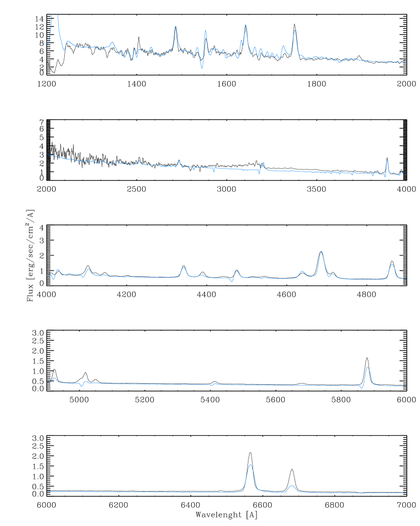
Figure 13: Comparison between the spectrum obtained on December 30, 1994 (black) and the sum of the current best model for star A at this epoch and star C model (blue). The singlet He I lines are underestimated while the triplet lines are well reproduced.

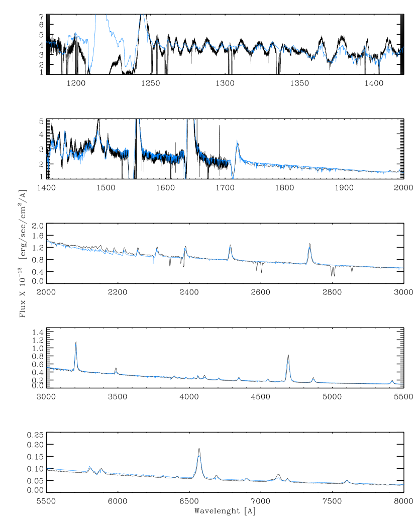
Figure 14: As if Fig. 13 but for the April 2000 epoch.

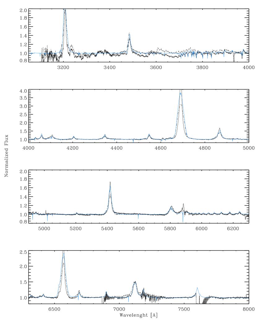
Figure 15: As in Fig. 11 but for the optical region. The spectrum is affected by the presence of strong telluric absorption lines in 6850Å, 7200Å and 7550Å. The observed profile of He II 4686Å and H_α is much narrower than the model spectrum. Breysacher et al. (1982) showed that He II 4686 Å  changes its profile with the orbital period being narrower at the eclipses. The model show that the line width outside the eclipse correspond to the UV P Cyg lines and there is missing emission during the eclipse. The interpretation of this effect requires a reliable model for star B which will be treated in a forthcoming paper.

Figure 16: Temperature distribution in the 1994 (solid line) and 2009 (dashed line) models. The positions of the sonic point and the continuum forming regions ($\tau_{Ross}$ = 2/3) are indicated. The lower mass loss rate in the 2009 model moves the continuum-forming region inward.

Figure 17: The relation between V_∞ and V_esc at different epochs.

References

- Arrieta et al. (2011) Arrieta,A., Hillier, D.J., Morisset, C., Georgiev, L., Stasinska, G., 2011, in preparation
- Barba and Niemela (1994) Barbá, R.H. & Niemela, V.S 1994,
- Barba and Niemela (1995) Barba, R. H., Niemela, V. S., Baume, G., & Vazquez, R. A. 1995, ApJ, 446, L23
- Barba et al. (1996) Barba, R. H., Morrell, N. I.; Niemela, V. S. et al.,1996, Revista Mexicana de Astronomia y Astrofisica Conference Series, 5, 85
- Barba et al. (1997) Barbá, R.H., Niemela, V.S., Morrell, N.I. 1997, “Luminous Blue Variables: Massive stars in Trnsition”, ed. A. Nota & H. Larmers, ASP Conf. Ser. 120, 238.
- Breysacher (1997) Breysacher, J. 1997, Luminous Blue Variables: Massive Stars in Transition, ASP Conf. Ser. 120, ed. A. Nota & H. Lamers, 227
- Breysacher (1982) Breysacher, J., Moffat, A.F.J. & Niemela, V. 1982, ApJ, 257, 116
- Breysacher (1980) Breysacher, J., & Perrier, C. 1980, A&A, 90, 207
- Cardelli (1989) Cardelli, J. A., Clayton, G. C., & Mathis, J. S. 1989, ApJ, 345, 245
- Colina (1996) Colina, L., Bohlin, F. & Castelli, F. 1996, Instrument Science Report CAL/SCS-008
- Crowther (2002) Crowther, P. A., Hillier, D. J., Evans, C. J., Fullerton, A. W., De Marco, O., & Willis, A. J. 2002, ApJ, 579, 774
- Drissen (2001) Drissen, L., Crowther, P.A., Smith, L.J., Robert, C., Roy, J.-R.,& Hillier, D.J. 2001, ApJ 545, 484.
- Dufau (2002) Dufau, S., Ruiz, M.,T., 2002, private communication.
- Dufour (1984) Dufour, R. J. 1984, Structure and Evolution of the Magellanic Clouds, 108, 353
- Dwarkadas (2011) Dwarkadas, V. V. 2011, MNRAS, 412, 1639
- Eenens (1994) Eenens, P.R.J. & Williams, P.M. 1994, MNRAS, 269, 1082.
- Foellmi (2008) Foellmi, C., et al. 2008, Rev. Mexicana Astron. Astrofis., 44, 3
- Georgiev (2004) Georgiev, L. N., & Koenigsberger, G. 2004, A&A, 423, 267
- Grafener (2008) Gräfener, G., & Hamann, W.-R. 2008, A&A, 482, 945
- Grevesse (2007) Grevesse, N., Asplund, M., & Sauval, A. J. 2007, Space Sci. Rev., 130, 105
- Groh (2009) Groh, J. H., Hillier, D. J., Damineli, A., et al. 2009, ApJ, 698, 1698
- Guzik (2005) Guzik, J. A., Cox, A. N., & Despain, K. M. 2005, The Fate of the Most Massive Stars, 332, 263
- Heydari-Malayeri (1997) Heydari-Malayeri, M., Rauw, G., Esslinger, O., & Beuzit, J.-L. 1997, A&A, 322, 554
- Herald (2011) Herald, J., Bianchi, L., 2011, MNRAS, submitted.
- Hilditch (2005) Hilditch, R. W., Howarth, I. D., & Harries, T. J. 2005, MNRAS, 357, 304
- Hillier (1998) Hillier, D.J., Miller,D, 1998, ApJ, 496,407
- Hillier (2003) Hillier, D. J., Lanz, T., Heap, S. R., Hubeny, I., Smith, L. J., Evans, C. J., Lennon, D. J., & Bouret, J. C. 2003, ApJ, 588, 1039
- Hunter (2007) Hunter, I.; Dufton, P. L.; Smartt, S. J.; Ryans, R. S. I.; Evans, C. J.; Lennon, D. J.; Trundle, C.; Hubeny, I.; Lanz, T. 2007, A&A, 466, 277
- Jones (1997) Jones, A., & Sterken, C. 1997, Journal of Astronomical Data, 3, 3
- Kashi (2010) Kashi, A. & Soker, N., 2010, ApJ, 723, 602.
- Koenigsberger (2004) Koenigsberger, G. 2004, Rev. Mexicana Astron. Astrofis., 40, 107
- Koenigsberger (1987) Koenigsberger, G., Moffat, A.F.J., & Auer, L. H. 1987, ApJL, 322, L41.
- Koenigsberger (1994) Koenigsberger, G., Moffat et al. 1994, ApJ, 436, 301.
- Koenigsberger (1995) Koenigsberger, G., Guinan, E., Auer, L., & Georgiev, L. 1995, ApJ, 452, L107
- Koenigsberger (1996) Koenigsberger, Shore, Guinan, Auer, 1996, RMAACS, 5, 92.
- Koenigsberger (1998) Koenigsberger,G., Auer,L.H., Georgiev,L. and Guinan, E. 1998, ApJ, 496,934.
- Koenigsberger (1999) Koenigsberger, G., Pena, M., Schmutz, W., & Ayala, S. 1998b, ApJ, 499, 889
- Koenigsberger (2000) Koenigsberger, G., Georgiev, L., Barbá, R., Tzvetanov, Z., Walborn, N. R., Niemela, V. S., Morrell, N., & Schulte-Ladbeck, R. 2000, ApJ, 542, 428
- Koenigsberger (2001) Koenigsberger, G., Georgiev, Leonid; Peimbert, Manuel; Walborn, Nolan R.; Barb , Rodolfo; Niemela, Virpi S.; Morrell, Nidia; Tsvetanov, Zlatan; Schulte-Ladbeck, Regina 2001, AJ, 121, 267
- Koenigsberger (2002) Koenigsberger, G., Kurucz, R., Georgiev, L. 2002, ApJ, 581, 598.
- Koenigsberger (2006) Koenigsberger, G., Fullerton, A., Massa, D. & Auer, L.H. 2006, AJ, 132, 1527.
- Koenigsberger (2010) Koenigsberger, G., Georgiev, L., Hillier, D.J., Morrell, N., Barbá, R., Gamen, R. 2010, AJ, 139, 2600
- Kudritzki (1995) Kudritzki, R.-P., Lennon, D. J., & Puls, J. 1995, Science with the VLT, 246
- Lamers (1995) Lamers, H. J. G. L. M. 1995, IAU Colloq. 155: Astrophysical Applications of Stellar Pulsation, 83, 176
- Lamers (1999) Lamers, H. J. G. L. M., & Cassinelli, J. P. 1999, Introduction to Stellar Winds, Cambridge, UK: Cambridge University Press, June 1999.,
- Lamers (1996) Lamers, H. J. G. L. M., Snow, T. P., & Lindholm, D. M. 1995, ApJ, 455, 269
- Lamers (2002) Lamers, H. J. G. L. M., & Nugis, T. 2002, A&A, 395, L1
- Maiz-Apellaniz (2005) Maíz-Apellaniz, J. & Bohlin, R.C. 2005, Space Telescope Science Institute,Instrument Science Report STIS 2005-01
- Moffat (1998) Moffat, A. F. J., Marchenko, S. V.; Bartzakos, P.; Niemela, V. S.; Cerruti, M. A.; Magalhaes, A. M.; Balona, L.; St-Louis, N.; Seggewiss, W.; Lamontagne, R. 1998, ApJ, 497, 896
- Morisset (2009) Morisset, C., & Georgiev, L. 2009, A&A, 507, 1517
- Nichols (1996) Nichols, J. S. & Linsky, J. L. 1996, AJ, 111, 517.
- Niemela (1988) Niemela, V.S., 1988, ASPCS 1, 381.
- North (2010) North, P., Gauderon, R., Barblan, F., & Royer, F. 2010, A&A, 520, A74
- Nugis (2002) Nugis, T., & Lamers, H. J. G. L. M. 2002, A&A, 389, 162
- Owocki (2008) Owocki, S., & van Marle, A. J. 2008, IAU Symposium, 250, 71
- Peimbert (2000) Peimbert, M., Peimbert, A., & Ruiz, M. T. 2000, ApJ, 541, 688
- Perez (1992) Perez, M. 1992, NASA IUE Newsletter 48, 76.
- Perrier (2009) Perrier, C., Breysacher, J., & Rauw, G. 2009, A&A, 503,963.
- Pojmanski (2002) Pojmanski, G. 2002, Acta Astronomica, 52,397
- Prinja (1990) Prinja, R.K., Barlow, M.J., & Howarth, I.D. 1990, Apj, 361, 607
- Schmutz (1989) Schmutz, W., Hamann, W.-R., & Wessolowski, U. 1989, A&A, 210, 236
- Schweickhardt (2000) Schweickhardt, J. 2000, PhD Thesis, Ruprecht-Karls-Universität, Heidelberg.
- Smith (2004) Smith, N., Vink, J. S., & de Koter, A. 2004, ApJ, 615, 475
- Smith (2008) Smith, N. 2008, IAU Symposium, 250, 193
- Sterken (1997) Sterken, C. & Breysacher, J. 1997, A&A, 328, 269.
- van Marle (2007) van Marle, A. J., Langer, N., & García-Segura, G. 2007, A&A, 469, 941
- Vink (1999) Vink, J. S., de Koter, A., & Lamers, H. J. G. L. M. 1999, A&A, 350, 181
- Vink (2011) Vink, J. S., Muijres, L. E., Anthonisse, B., de Koter, A., Graefener, G., & Langer, N. 2011, arXiv:1105.0556