Non-Gaussian Error Bars in Galaxy Surveys (Part 1)
Abstract
We propose a method to estimate non-Gaussian error bars on the matter power spectrum from galaxy surveys in the presence of non-trivial survey selection functions. The estimators are often obtained from formalisms like FKP and PKL, which rely on the assumption that the underlying field is Gaussian. The Monte Carlo method is more accurate but involves the tedious process of running and cross-correlating a large number of N-body simulations, in which the survey volume is embedded. From 200 N-body simulations, we extract a non-linear covariance matrix as a function of two scales and of the angle between two Fourier modes. All the non-Gaussian features of that matrix are then simply parametrized in terms of a few fitting functions and Eigenvectors. We furthermore develop a fast and accurate strategy that combines our parameterization with a general galaxy survey selection function, and incorporate non-Gaussian Poisson uncertainty. We describe how to incorporate these two distinct non-Gaussian contributions into a typical analysis pipeline, and apply our method with the selection function from the 2dFGRS. We find that the observed Fourier modes correlate at much larger scales than that predicted by both FKP formalism or by pure N-body simulation in a “top hat” selection function. In particular, the observed Fourier modes are already per cent correlated at , and the non-Gaussian fractional variance on the power spectrum () is about a factor of larger than the FKP prescription. At , the deviations are an order of magnitude.
keywords:
Large scale structure of Universe – Surveys – Dark matter – Distance Scale – Cosmology : Observations – Methods: data analysis1 Introduction
With new galaxy surveys probing a larger dynamical range of our Universe, our ability to constrain cosmological parameters is improving considerably. In particular, one of the most important goal of modern cosmology is to understand the nature of dark energy (Albrecht et al., 2006), a challenging task since there are currently no avenues to observe it directly. It is however possible to probe its dynamics via its equation of state , which enters in the Friedmann equation that governs the expansion of the Universe. Among different ways can be measured, the detection of the baryonic acoustic oscillations (BAO) dilation scale (Eisenstein et al., 2005; Tegmark et al., 2006; Hütsi, 2006; Percival et al., 2007; Blake et al., 2011) is one of the favorite, both because of the low systematic uncertainty and the potentially high statistics on can achieve with current (Huchra et al., 1990; York et al., 2000; Colless et al., 2003; Drinkwater et al., 2010) and future galaxy surveys (Peterson et al., 2006; Acquaviva et al., 2008; Schlegel et al., 2009; LSST Science Collaborations et al., 2009; Benítez et al., 2009; Beaulieu et al., 2010).
The strength of the BAO technique relies on an accurate and precise measurement of the matter power spectrum, whose uncertainty is propagated on to the dark energy parameters via a Fisher matrix (Tegmark, 1997). It is thus of the utmost importance to have optimal estimators of both the mean and the uncertainty of the power spectrum to start with. The prescription to construct an estimator for the power spectrum of a Gaussian random field, in a given galaxy survey, was pioneered by Feldmann, Kaiser and Peacock (Feldman et al., 1994) (FKP for short). It states that the survey selection function effectively couples Fourier bands that are otherwise independent, and that the underlying power should then be deconvolved (Sato et al., 2011). This technique has been used in power spectrum measurement such as (Feldman et al., 1994; Percival et al., 2001; Cole et al., 2005; Hütsi, 2006; Blake et al., 2010). Although it is fast, the error bars between the bands are correlated, plus it has the undesired tendency to smear out the underlying power spectrum, which can effectively reduce the signal-to-noise ratio in a BAO measurement. In that sense, the FKP power spectrum is said to be suboptimal.
The band correlation induced by the FKP prescription can be removed by an Eigenvector decomposition of the selection function, following the Pseudo Karhunen-Loève formalism (Vogeley & Szalay, 1996)(PKL). This was used in the analysis of the SDSS data (Tegmark et al., 2006) and is the most optimal (i.e. loss-less) estimator of a convolved Gaussian random field, as understood from the information theory point of view. It is nevertheless a well known fact that this Gaussian assumption about the field is only valid in the linear regime, since the non-linear gravitational collapse of the density effectively couples different Fourier modes together (Meiksin & White, 1999; Rimes & Hamilton, 2005), and the phases of the modes are no longer random (Coles & Chiang, 2000). Both the FKP and PKL prescriptions, by their Gaussian treatment, do not take into account the intrinsic non-linear coupling of the Fourier modes. It follows from this that for both methods, the measured power spectrum is suboptimal and the error bars are systematically biased. Although the bias is usually small, it causes a problem when estimating derived quantities that need to be measured with a percent level accuracy.
For instance, the observed BAO signal sits right at the transition between the linear and the non-linear regime, therefore the optimal estimator of the power spectrum must incorporate the non-linear modes. In particular, constraints on dark energy from BAO measurements require an accurate measurement of the matter power spectrum covariance matrix. Under the FKP and PKL formalisms, the covariance matrix is biased as it tends to underestimate the uncertainty and the amount of correlation between the power bands. Alternative ways of estimating the error, i.e. methods that involve mock catalogs, do model these non-linear dynamics, but it is not clear that the results are precise enough to measure four-points statistics, and we rather rely on accurate N-body simulations.
Even more relevant is the recent realization that an optimal, i.e. non-Gaussian, estimate of the BAO dilation scale requires a precise measurement of the inverse of the matrix, which is challenging due the noisy nature of the forward matrix. It was nevertheless shown that, first, a suboptimal measurement of the power spectrum should be accompanied with error bars that treat the mean as suboptimal by consistency. These error bars differ from the naive Gaussian approximation by a significant amount (Ngan et al., 2011). Second, it was shown in the same paper that an optimal measurement of the mean power spectrum could lead to an optimal measurement of the error, which differs from suboptimal measurements by a few percent. To achieve this, however, one needs to include the non-linear dynamics at a high precision, and needs in addition a strategy to cope with the noise present in the covariance matrix.
There are thus two aspects of the analysis that need to be extended from the above conclusions. On one hand, one would like to get rid of the aforementioned bias on the estimated uncertainty in actual data analyses, in which non-trivial survey selection function play a complex role. On the other hand, one would like to measure optimal error bars on the matter power spectrum of (non-Gaussian) galaxy fields. In this paper, we address the first issue, and provide a strategy to measure suboptimal but unbiased error bars on the power spectrum of galaxy surveys. It should be mentioned that our method could be put in conjunction with the PKL formalism to address the second issue, hence optimal measurement of both the power spectrum and of its error are now within reach.
When constructing an estimator of the covariance matrix that corresponds to the sensitivity of a particular survey, the convolution with the survey selection function is one of the most challenging part. Whereas the convolution of the underlying power spectrum can be operated with angle averaged quantities, the convolution of the covariance matrix must be done in 6 dimensions, since the underlying covariance is not isotropic: Fourier modes with smaller angular separations are more correlated than those with larger angles (Chiang et al., 2002; Bernardeau et al., 2002). The first challenge is to measure accurately this angular correlation, which is also scale dependent. Neither second order perturbation theory nor log-normal densities have been shown to calculate this quantity accurately, hence we must therefore rely on N-body simulations. This requires a special approach, since a naive pair counting of all Fourier modes in the four-point function, at a given angle, would take forever to compute. The second challenge comes from the 6-dimensional convolution of the covariance matrix with the survey function. This is a task that current computer clusters cannot solve by brute force, so we must find a way to use symmetries of the system and reduce the dimension of the integral. The fact is that the underlying covariance really depends only on three variables: two scales and the relative angles between the two Fourier modes. Moreover, it turns out, as we describe in section 6, that it is possible to express this matrix into a set of multipoles, each of which can further be decomposed into a product of Eigenvectors. This effectively factorizes the three dimensions of the covariance, hence the convolution can be broken down into smaller pieces. By doing so, the non-Gaussian calculation is within reach, and we present in this paper the first attempt at measuring deviations from Gaussian calculations, including both Poisson noise and a survey selection function. In short, the main ideas of this paper can be condensed as follow:
-
1.
The underlying non-linear covariance matrix of the matter power spectrum exhibits many non-Gaussian features in the trans- and non-linear regimes. First, the diagonal elements of the angle-averaged covariance grow stronger, and correlation across different scales becomes important. Second, Fourier modes with similar (or identical) magnitudes correlate more if the angle between them is small.
-
2.
It is possible to model all of these non-Gaussian aspects (including the dependence on the angle between the two Fourier modes) with a small number of simple functions.
-
3.
With such a parameterization, it is possible, for the first time, to solve the six-dimensional integral that enters the convolution of the covariance of the power spectrum with the galaxy survey selection function.
Concerning the second point, the parameters that best fit our measurements are provided in section 7, but these are separately testable, and could be verified by other groups and with other ways. These are anyway expected to change when one uses haloes instead of particles. The third point is, however, a straight forward recipe that is robust under possible changes of best-fitting parameters, and provides, assuming that the input parameters are correct, an unbiased measurement of the non-Gaussian uncertainty of the matter power spectrum.
As indicated by the title, this paper is the first part of a general strategy that aims at constructing an unbiased, non-Gaussian estimator of the uncertainty on the matter power spectrum measured in galaxy survey. The second part, which we thereafter refer to as HDP2 (in preparation), exploits the fact that the measurement of the matrix provides a novel handle at measuring : the two quantities are related by a straight forward integration over . As shown in a later section of the current paper, it turns out that the main contribution to comes from small separation angles, while larger angles are noise dominated. It is thus possible to perform a noise weighted integral, which results in a more optimal measurement of and of its error bars, compared to direct or bootstrap sampling. It is therefore possible to extract an accurate non-Gaussian error bar on the power spectrum with a much smaller number of realizations. This opens the door for a measurement of a non-Gaussian covariance matrix directly from the data (i.e. an internal estimate), a significant step forward in the error analysis of galaxy surveys. In that second part, we will first test the improvement of the noise-weigthed technique on the same 200 simulations. We will then attempt to extract the mean and the error on all the elements of the matrix from a mock survey, that will consist of a handful of simulations.
Back to the current paper, our first objective is thus to measure the covariance of the power spectrum between various scales and angles, and organize this information into a compact matrix, . We describe how we solve this problem in a fast way, which is based on a series of fast Fourier transforms and that can be run in parallel on a large number of computers. We found that the angular dependence, at fixed scales (), is rather smooth, it agrees with analytical predictions in the linear regime, but deviates importantly from Gaussianity for smaller scales. The dependence is somehow similar when the two scales are identical, up to an delta function for vanishing angles. We also found that, once projected on to a series of Legendre polynomials, it take very few multipoles to describe the complete original function. We perform this transform for all scale combinations and group the results in terms of the multipole moments. We also provide a recipe to reconstruct the original covariance matrix, with the angular dependence, from a handful of fitting functions. This is another advantage of the method we propose here: it can be separately tested and improved.
Our second objective is to provide a general method to combine this with a survey selection function and non-Gaussian Poisson noise, and hence allow the extraction of non-Gaussian error bars on the measured power spectrum. We test our technique on the publicly available 2dFGRS selection functions (Norberg et al., 2002) and find that there is a significant departure between the Gaussian and non-Gaussian treatment. In particular, the fractional error of the power spectrum () at is about a factor of 3.0 higher in the non-Gaussian analysis, and the departure reaches an order of magnitude by . The method proposed here can be also applied to other kinds of BAO experiments, including intensity mapping from the emission of the 21 cm line by neutral Hydrogen (Peterson et al., 2006; Lazio, 2008; Schlegel et al., 2009), or Lyman- forests surveys (McDonald & Eisenstein, 2007; McQuinn & White, 2011). We did not, however, include the effect of redshift distortions, and focused our efforts on dark matter density fields obtained from simulated particles. An improved version of this work would include both of these effects, however.
This paper is organized as follow: In section 2, we briefly review the FKP method, and describe how to estimate non-Gaussian error bars in realistic surveys, given a previous knowledge of . We then lay down the mathematical formalism that describes how we extract this quantity from simulated density fields in section 3. Section 4 contains the results from sanity checks and null tests that were performed to validate our method, and briefly describes our N-body simulations. We present our measurement of in section 5, and describe the multipole decomposition in section 6. In section 7, we further simplify the results by extracting the principal Eigenvectors and provide fitting formulas to reconstruct easily the full covariance matrix. Section 8 contains results of applying our method for a set of simple selection functions. We finally discuss some implications and extensions of our methods in 9, and conclude in section 10.
2 Matter Power Spectrum from Galaxy Surveys
In this section, we quickly review the general FKP method, which is commonly used in data analysis (Feldman et al., 1994; Percival et al., 2001; Blake et al., 2010). We then point out some of the major the flaws of such techniques when measuring the uncertainty, and describe how non-Gaussian error bars could be estimated in principle. Before moving on, though, we first lay down the conventions used throughout the paper. The reader familiar with the FKP method may skip to section 2.2.
A continuous density field is related to its Fourier transform by
| (1) |
where is the wave number corresponding to a given Fourier mode. The power spectrum of the field is defined as:
| (2) |
and is related to the mass auto-correlation function by :
| (3) |
In the above expressions, the angle brackets refer to a volume average in Fourier space, and stands for the Dirac delta function.
2.1 The optimal estimator of the power spectrum
The power spectrum of the matter field contains a wealth of information about the cosmic history and the principal constituents of the Universe. Unfortunately, it is not directly detectable, since our observations are subject to cosmic variance, detection noise, light to mass bias, redshift distortions and incomplete sky surveys. The FKP method provides an optimal estimator of the matter power spectrum under the assumption that the density field is Gaussian. It is formulated in terms of the survey selection function , the galaxy number density , the dimensions of the grid where the Fourier transforms are performed, and the actual number count per pixel . All the following calculations can be found in (Feldman et al., 1994), and are included here for the sake of completeness.
The first step is to construct series of weights as
| (4) |
where , is the mean galaxy density and is a characteristic amplitude of the power spectrum at the scale we want to measure. Since the latter is not known a priori, it is usually obtained from a theoretical model, and sometimes updated iteratively. The selection function is also normalized such that .
The optimal estimator of the power spectrum, , is obtained first by re-weighting each pixel by the weights in [Eq. 4], then by subtracting from the result a random catalog with the same selection function, weights and number of objects . After taking the expectation value of the results, the 2-points statistics of the pixel counts becomes
| (5) |
where is the mean density in the patch over which the average is performed. The Fourier transform is then given by
| (6) |
where denominator is a convenient normalization. This measured power is aliased by the grid mass assignment scheme, and should be divided by the appropriate function (Jing, 2005).
What this estimator measures is not the underlying power spectrum , but a convolution with the survey selection function:
| (7) |
It ideally needs to be deconvolved, an operation that is not always possible.
For many survey geometries, the convolution effectively transfer power across different bins which are uncoupled to start with (Tegmark et al., 2006). As mentioned previously, the PKL prescription also assumes that the density field is Gaussian, but rotates into a basis in which the bins are decoupled. In that sense, the PKL technique is more optimal than the FKP, unless the selection function is close to a “top hat”, in which case the induced mode coupling vanishes. Both case, however, rely on the fundamental assumption that the underlying density field is Gaussian, which is known to be inaccurate in the trans- and non-linear regime, where one still wants an accurate measure of the power spectrum for a BAO analysis. Obtaining accurate error bars is a requirement for optimal analyses, and we shall examine how these are usually obtained.
2.2 The FKP covariance matrix
The covariance matrix of the angle averaged power spectrum is a four point function that contains the information about the band error bars, and possible correlation between them. As mentioned earlier, it is required for many cosmological parameter studies. It is generally obtained from the power spectrum as
| (8) |
where refers to the fluctuations of the measured values about the mean, which is ideally obtained from averaging over many realizations. In a typical galaxy survey, such independent realizations are obtained by sampling well separated patches of the sky. Because of the cost of such an operation, the number of patches is usually very small. The covariance matrix is thus not resolved from the data, and the error bars are obtained with external techniques, i.e. from mock catalogs111We post-pone the discussion of mock catalogs until the next section, or directly from Gaussian statistics (see HDP2 for a prescription that overcomes this challenge). For a uniform (top-hat) selection function, the Gaussian covariance matrix is estimated as:
| (9) |
where and is the number of Fourier modes that enters in the measurement of . In the ideal scenario of perfect spherical symmetry and resolution, , with being the width of the -band. The Kronecker delta function ensures that there is no correlation between different modes, an inherent property of Gaussian random fields. This equation can be easily be modified to deal with measurements without angle averaging.
The FKP prescription provides a generalization of [Eq. 9] for the case where the selection function varies across the volume. It is obtained from [Eq. 6] and given by
| (10) |
where
| (11) |
| (12) |
In [Eq. 10], is taken to be the mean of the power spectrum at separation . Because the selection functions are usually quite compact about , that approximation is reasonable for Gaussian fields. Also, [Eq.9] can be recovered by setting .
2.3 Non-Gaussian error bars
As mentioned in the last section, it is necessary to have access to many realization of the matter field in order to measure a non-Gaussian covariance matrix of power spectrum. This could in principle be done from data across many different patches in the sky, but even then, we have only one sky to resolve the largest modes, which would therefore be dominated by cosmic variance. Not to mention the cost and time involved in measuring many large but disconnected volumes. Fortunately, N-body simulations are now accurate and fast enough to generate large numbers of measurements of the matter power spectrum. Since they model the non-linear dynamics of structure growth, the density fields they generate are non-Gaussian. The covariance matrix constructed from a high number of simulations indeed shows a correlation across different scales in the non-linear regime (Meiksin & White, 1999; Rimes & Hamilton, 2005; Takahashi et al., 2009; Ngan et al., 2011).
Although much more representative of the underlying covariance, such matrices are hard to incorporate in a data analysis, first because they are based on a fixed set of cosmological parameters, but also because the simulated volume is cubic and periodic. Each survey group typically needs to run at least one N-Body simulation, and measure the power spectrum with and without the measured selection function, in order to quantify the bias of their measurement. The complete approach would then be to run hundred of these to measure the covariance matrix, and to repeat for a range cosmological parameters values. This whole procedure is expensive, which explains why it is never done in practice. The alternative is to use mock galaxy catalogs, obtained, for example, from log normalization of Gaussian densities, second order perturbation theory (PT), haloPT, and so on. Unfortunately, the accuracy of such techniques at modeling the four-point functions and angle dependencies has not been fully quantified.
Another artefact of the simulations is that the number of particles can be arbitrary adjusted such as to suppress the Poisson noise down to a level where it is negligible. This is certainly not true for many galaxy survey, in which the number density is often much lower. We measure a non-Gaussian Poisson error by sampling random fields with a selection threshold chosen as to mimic the number density of a realistic survey, and incorporate the effect manually in the analysis, as explained in section 8.
To measure non-Gaussian error bars on a realistic survey, the most accurate procedure would be to convolve the best available estimator of the covariance matrix with the selection function. Because the later is generally not spherically symmetric, it is the full 6-dimensional covariance matrix, , that needs to be integrated over. Let us suppose, for a moment, that we successfully measured that complete non-Gaussian covariance matrix. It would first contain an element for each Fourier modes (i.e. with no angular averaging), and from [Eqs. 7 and 8], we can write:
| (13) | |||||
where the angled bracket is nothing else but that full covariance matrix . We can then simplify the result since the covariance between two Fourier modes depends only the angle between them, but not on the absolute orientation of the pair in space. In other words, we make use of this symmetry argument to write without lost of generality. This angle can further be expressed in terms of the two angles made by and as
| (14) |
We show in a later section of this paper that the true covariance matrix can be decomposed into a sum of factorized terms, each of the form . So the double convolution of [Eq. 13] can actually be broken into a sum of smaller pieces, with at most 3-dimensional integrals to perform.
This sets the path of this paper. We propose in the next section a novel technique to measure , we next present the results, and we finally perform the convolution on a realistic survey selection functions.
3 Measuring the Angular Dependence: the Method
As mentioned above, our first objective is to extract the covariance matrix of the power spectra from N-Body simulations, as a function of two scales and one angle: . In this section, we develop a novel way to obtain covariances and cross-correlations and which allows us to perform this measurement.
3.1 Cross-correlations from Fourier transforms
We start by assuming we have measured the power spectrum from a large number of simulations. We first compute the mean of the angle averages: and the deviation from the mean of each mode:
| (15) |
We then select two scales, and , that we want to cross-correlate. We make two identical copy of three-dimensional power spectra and multiply each one by a radial top hat function corresponding to the particular scales:
| (16) |
where is the product of two Heaviside functions. Also, is the shell thickness, taken to be very small. We then cross-correlate the subsets and define:
| (17) |
We then express both ’s in [Eq. 17] in terms of their mass auto-correlation functions . We first integrate over and obtain a delta function, which allows us to get rid of one of the real space integral. After slightly rearranging the terms, we obtain:
| (18) |
In the above equation, can be expressed as:
| (19) | |||||
Since the shells we select are very thin, we can safely approximate that the power spectrum is constant over the infinitesimal range, and thus perform the integral:
| (20) |
We next repeat the same procedure for a scale , multiply both auto-correlation functions together, and Fourier transform the product, following [Eq. 18]. The result is the cross-correlation , which becomes, after performing the integral over the plane wave:
| (22) | |||||
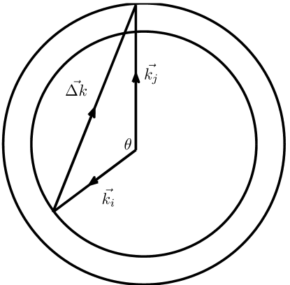
The delta function enforces to point from to , which span the shells and respectively in the integrals over the solid angles. This geometry allows us to use the cosine law and relate to the angle it subtends, as seen in Fig. 1, such that:
| (23) |
Since many subtend the same angle , we can perform an average over them and compute
| (24) |
3.2 Normalization
The quantity is not exactly equal to , because there is a subtle aliasing effect which is purely geometrical, and which needs to be canceled. To see how this arises, we work out a very simple scenario, in which the density field is perfectly isotropic. In that case, we can write , hence the angular integration in [Eq.20] is straight forward and we get:
| (25) |
with the zeroth order spherical Bessel function. We have also assigned to the shell thickness, which corresponds to the resolution of a simulation of side . Then, [Eq.18] becomes
| (26) |
where
| (27) |
The function is independent of the actual power spectrum; it is purely a geometrical artifact, and we discuss in Appendix A its meaning. However, a power spectrum that is exactly isotropic should have no angular dependence.We thus define a normalization , as the output of [Eq. 24] with everywhere on the shells. The final results is obtained by dividing off this normalization, which cancels off the geometrical effect:
| (28) |
We stress again that this result is an average over all configurations satisfying . To summarize, here is a condensed list of the steps taken to measure :
-
1.
Measure the mean angle averaged from an ensemble of simulations,
-
2.
Select a combination of shells to cross-correlate,
-
3.
For each simulation, compute , duplicate and multiply each replica by a top hat , which effectively sets to zero every off-shell grid cells,
-
4.
Subtract from each cells in the shell,
-
5.
Fourier transform both grids, complex multiply them, and Fourier transform back to -space,
-
6.
Loop over the available, bin into , and express the result as a function of ,
-
7.
Repeat steps 5-6, but this time assigning the value of each cell in the shell to unity. Divide by this normalization. This is a measure of from one simulation,
-
8.
Repeat for all simulations, then compute the mean,
-
9.
Iterate over steps 2-8 for other shell combinations.
To achieve better results, we make use of the fact that , hence, following [Eq.17], we can write . This translates into a theoretical symmetry about in the angular dependence of the covariance. That property turns out to be very useful at reducing the numerical noise, since we can measure the covariance over the full angular range, but fold the results on to . Also, to avoid interpolating error, we chose to bin in before transforming to .
3.3 Zero-lag point
It is important to note that for a given realization, the point at , which we refer to as the zero-lag point, must be treated with care. We recall from [Eq. 19] that for a given simulation, we subtract the mean from every points which are on the specified -shell (and the other points are set to zero); we repeat the same procedure on a second -shell, and we then cross-correlate the two fields.
When the two shells are identical, i.e. , the zero-lag point of each simulation first computes the square of the deviation the mean , then averages the result over the whole shell. It is equivalent to calculating the variance over the shell, but using a mean which is is somewhat off from the actual mean on that shell. That effectively boosts the variance. When we average over all simulations, the zero-lag points can be written as:
| (29) |
where, in the first term, the angle average and mean over all realizations are computed after squaring each grid cell. By comparison, the variance on angle averaged power spectra would be obtained by performing, in the first term, the angle averaging first, then taking the square, then taking the mean.
On the other hand, when the two shells are different, the zero-lag point is now the average over on both shells. Since we are no longer squaring each terms, it now includes negative terms, hence is generally of much smaller amplitude.
4 Validation of the Method
We describe in this section a series of tests that compare our numerical results to semi-analytical solutions. We apply our numerical methods on a few simple situations in which we control either the density field or the three dimensional power spectrum. We first test our recipe on a power spectrum that is set to the second Legendre polynomial. The outcome can be compared to semi-analytical calculations and gives a good grip on the precision we can achieve. We next measure the angular dependence of the covariance matrix of white noise densities by Poisson sampling many random distributions, and present an estimate for a non-Gaussian Poisson error See (Cohn, 2006) for discussions of these two types of noise in a cosmological context. We finally measure the angular cross-correlation from Gaussian random fields in order to later measure departures from Gaussianity.
4.1 Testing with a Legendre polynomial
As a first test, we enforce the -dependence of the power spectrum to be equal to the second Legendre polynomial, and then compare our results to semi-analytic predictions. We manually set , which is thus constant across the plane. The mean and the deviation from the mean on a shell are given by , respectively, where is the -th Legendre polynomial and is the cosine of the inclination angle. The mass auto-correlation function associated with this power is
| (30) |
The angular dependence of the covariance can be calculated semi-analytically from Eq.18 and the above mass auto-correlation function. The angular integration is straight forward, and we obtain
| (31) |
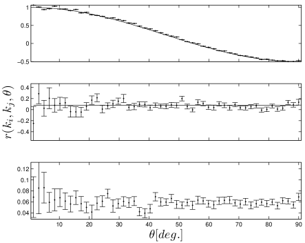
We perform the integral with , repeat the procedure for , and obtain a semi-analytical prediction: , up to numerical noise. This agrees well with the numerical results produced by our technique, as shown in the top part of Fig. 2. We are plotting the angle-dependence of the covariance matrix, normalized by the angle average of the covariance, such that the curve represents the actual cross-correlation coefficient between the Fourier modes. We mention here that in the case where , which we encounter in the following sections, we normalize to the square root of the product of the corresponding matrix elements:
| (32) |
In the particular case under study in this section, the Fourier modes separated by small angles are strongly correlated by construction.
4.2 Testing with Poisson-sampled random fields
To measure the response of our code to white noise, we produce a set of density field representing Poisson sampling of random distributions. The sensitivity threshold is chosen such that peaks were counted on average. The standard deviation in the measured decreases roughly as , expected from the fact that the number of cells on a -shell grows as .
Because of the random nature of Poisson density, the variance on a given shell should be roughly constant across all directions. Moreover, after averaging over many realization, Poisson densities are in principle statistically isotropic. We thus expect the measured angular dependence of the covariance to be very close to flat, and, from [Eq.28], we estimate it should plateau at a value somewhat similar to the covariance of angle averaged power spectrum, :
| (33) |
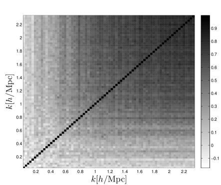
where and the two delta functions ensure that modes with different directions or scales do not couple together. Also, is obtained directly from the covariance matrix of the angle average power spectra. The constant is much larger than , for reasons explained in section 3.3, but the precise value is irrelevant to the current analysis. Fig. 3 shows the cross-correlation coefficient matrix for non-Gaussian Poisson noise. We observed that the angle-averaged modes are correlated by more than per cent between scales smaller than . The reason for this feature is actually independent of cosmology, even though the matrix has a look very similar to that measured from simulations222It is in fact arguable that such a matrix, constructed from a set of Poisson densities, could have better performances at modeling the ‘true’ non-Gaussian covariance matrix, compared to the naive Gaussian approximation. . The explanation lies in the fact that our Poisson densities do not have exactly the same number of objects, hence the asymptotic value of is not a perfect match for all field. This slight scatter in power translates into a correlation between the high modes of a given density field, and we use this matrix to estimate the non-Gaussian Poisson noise. This is in good agreement with the predictions of (Cohn, 2006), which calculated that the Poisson sampling of Gaussian fields induce non-Gaussian statistics, and that well separated scales can correlate significantly.
We then measure the angular dependence of the covariance for these Poisson distributions, also at . We obtain a distribution which is indeed close to flat, and consistent with a uniform per cent correlation, as shown in the middle plot of Fig. 2. As before, we have normalized the plot by the angle averaged covariance matrix element, such as to exhibit the angular cross-correlation. Because the zero-lag point is typically a few orders of magnitude above the other points, we quote its value in the text or in the figures’ caption where relevant, and resolve the structure of the other angles. The mean of the un-normalized distribution is , a per cent agreement with our rough estimate. We have re-binned the distributions on to a set of points that are optimal for the upcoming angular integration, as described in section 6.
4.3 Testing with Gaussian random fields
The next test consists in measuring the angular dependence of the covariance from of 200 Gaussian random fields. We use power spectra measured at , obtained from N-Body simulations (section 5.1), to generate 200 fields. Similarly to the Poisson fields, we expect the distribution to be be overall flat, except for the zero-lag point. Because we choose not to Poisson sample these Gaussian densities, the randomness should be such that near to perfect cancellation occurs between the different angles, and the plateau should be at zero. In the continuous case, the Gaussian covariance can be expressed as [Eq. 41], with
| (34) |
where is the number of Fourier modes in the -shell. For , the zero-lag point contains perfectly correlated power, so we expect it to have a very large value. As explained in section 3.3, we cannot directly compare its value to , since the former is bin dependent, while the latter is not. In the case where however, the zero-lag point should drop down to numerical noise.
The measured angular dependence is presented in the bottom part of Fig. 2, where we see that the distribution is flat and consistent with per cent correlation. This indicates that our method suffers from a small systematic bias and detects a small amount of correlation, in a angle independent manner. We have repeated this measurement for different scales and obtained the same bias. We therefore conclude that any signal which is smaller than this amount is bias dominated and not well resolved.
5 Measuring the Angular Dependence
In this section, we present the results obtained from the measurement of the angular covariance in our simulations.We explore different scale combinations and attempt to compare the outcome to expected results whenever possible. In particular, the linear regime should somewhat reproduce the behavior we observe in Gaussian random fields (see section 4.3). In all figures, the error bars were obtained from bootstrap re-sampling of our simulations, unless otherwise specified.
5.1 N-body simulations
Since our Universe is not Gaussian at all scales relevant for BAO or weak lensing analyses, a robust error analysis should be based on non-Gaussian statistics, and, as mentioned earlier, N-body simulations are well suited to measure covariance matrices. Our numerical method is fast enough that, for fixed and , we can compute the angular dependence of the covariance matrix in about one minute. The average over 200 realizations can be done in parallel, hence producing all available combinations takes very little time.
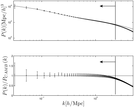
The simulations are produced by cubep3m(Merz et al., 2005), a public N-body code that is both openmp and mpi parallel, which makes it among the fastest on the market333http://www.cita.utoronto.ca/mediawiki/index.php/CubePM. We generate 200 Gaussian distributions of 200 Mpc per side, with particles, starting at , and evolved them until . The simulations are run on the CITA Sunnyvale cluster, a Beowulf cluster of 200 Dell PE1950 compute nodes, each equipped with 2 quad cores Intel(R) Xeon(R) E5310 @ 1.60GHz processors. Each node has access to 4GB of RAM and 2 gigE network interfaces. The power spectrum of these simulations is shown in Fig. 4, and shows a good agreement with the non-linear predictions from CAMB (Seljak & Zaldarriaga, 1996), up to . Beyond that scales the structures are under estimated due to the resolution limit of the simulations. For the rest of this paper, we only consider well resolved scales, in occurrence those in the range , which we organize into linearly spaced bins.
5.2 Results
We present in Figs. 5 and 6 the angular dependence of the covariance between the power spectrum of various scales. As explained in the previous section, the distributions are normalized such as to represent the cross-correlation coefficient between modes separated by an angle . In the first figure, both scales are selected to be identical, and vary progressively from to . Modes separated by an angle larger than are less correlated at all scales, and the correlation is even smaller for modes smaller than . These latter modes are grouped in larger bins due to the higher discretization of the shells, and ideally one would like to run another set of simulation at larger scales to have a better resolution on those scales. However, the modeling of these rather larger scales have very little impact on the non-Gaussian analysis we are carrying, we therefore do not attempt to improve the situation. For highly non-linear scales, the correlation between modes less than increases up to per cent.
In the second figure, one of the two scale is held constant, at , while the other varies over the same range. Modes separated by angles larger than are less than per cent correlated, for all combinations of scales. When the two scales are of comparable size, the the correlation climbs up to values between and per cent for angles smaller than .
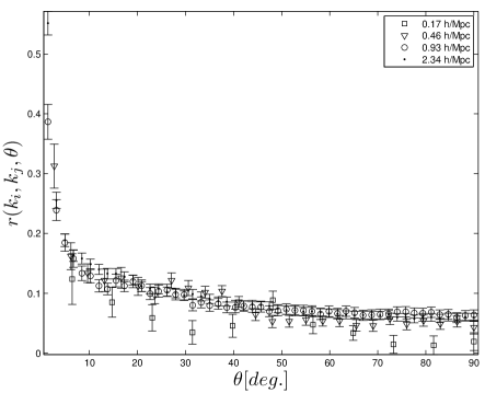
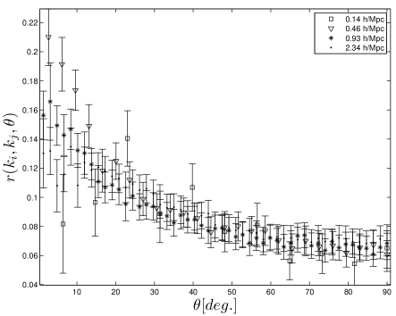
This angular behavior is enlightening, as it shows how the error between Fourier modes separated only by a small angle tend to correlate first. Qualitatively, this validate the fact that in non-Gaussian densities, quasi-parallel Fourier modes are probing essentially the same collapsed structures. When the angle is closer to , however, one mode could go along a filament and the other across it, producing only weak correlations. It could thus be possible to construct a highly clustered density in which we could observe an anti-correlation at , provided we are not noise dominated.
This coherent behavior is a clear sign that the non-linear structure underwent gravitational collapse, and the departure from Gaussianity and white noise is obvious. Another signature of non-Gaussianity is that even in the presence of a small offset between the scales, the small angle correlation has a value higher than those at larger angles, because of the coupling between those scales. Fig. 6 shows this effect.
5.3 From to
It is possible to recover the covariance matrix one obtains from the angle averaged by performing a weighted sum over the angular covariance444The weight here is simply the number of contribution that enter each angular bin, divided by the square of the total number of cells on the -shell. In other words, because the angular covariance we measure is an average over many pairs of cells, that average must first be undone, then the different angles are summed up, and we finally divide by the total number of contributions.. Another test of the accuracy of our method is thus to compare the two ways that measure . This is by far the least convenient way of measuring this matrix, and we perform this check solely for verification purposes.
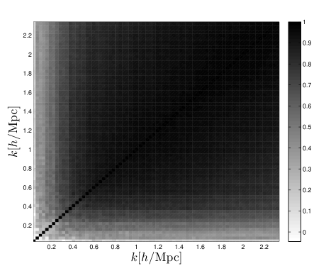
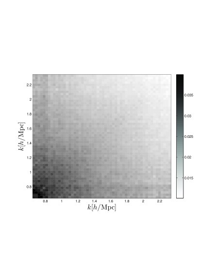
We perform this weighted sum and construct , then compute a similar matrix from our angle averaged power spectra. We present in Fig. 7 the cross-correlation coefficient matrix (see [Eq. 32]) obtained in the first way, and show the fractional error between both methods in Fig. 8. We observe that they agree at the few percent level, so long as we are in the non-linear regime. At very low -modes, however, many matrix elements are noisy due to the discretization of the shell; the mapping in this very coarse grid environment becomes unreliable, and the re-weighting hard to do correctly. This results in high fractional errors, but at the same time, this region is still in the regime where the analytic Gaussian prediction is valid. In addition, this paper attempts to solve the bias caused by the non-Gaussianities that lie in the trans-linear and non-linear regime, in which discretization effects are much smaller. Finally, we recall that these matrix elements have very little impact on most parameter studies since such scales contain almost no Fisher information (Rimes & Hamilton, 2005; Ngan et al., 2011).
6 Multipole Decomposition
As shown in last section, we have extracted the covariance matrix of matter power spectrum, cross-correlating the different scales selected. Since the final objective is to incorporate this massive object into generic data analysis pipelines, it must be somehow simplified or made more compact. A quick glance at the figures of section 5 reveals that the angular dependence of the covariance can be decomposed into a series of Legendre polynomials, in which only a few multipoles will bear a significant contribution. This allows us to rank the multipoles by importance and to keep only the dominant ones. These results are further simplified in section 7, where we provide fitting formulas to reconstruct .
In this section, we describe how we perform this spherical harmonic decomposition, then we test our method on the control samples described in section 4, and we finally measure the from the simulations.
6.1 From to
Here we lay down the mathematical relation between and . Let us first recall that the spherical harmonics can serve to project any function on to a set of as:
| (35) |
We substitute , which causes the coefficients to be scale dependent, i.e. . The angular power spectrum at a given angular size is defined as
| (36) |
Combining both equations, and writing to clarify the notation, we get
| (37) | |||||
We use the completion rule on spherical harmonics to perform the sum:
| (38) |
where is the angle between the and directions, and where are the Legendre polynomials of degree . We then write
| (39) |
Since we know that , we make a change of variable and rotate the prime coordinate system such that always points towards the -axis. In this new frame, we have , where is the angle subtended by . thus corresponds to the angle between the two Fourier modes and . It is also equal to in [Eq. 38].We perform the ‘unprime’ integral first, which gives
| (40) |
The inner integral is , we rename and obtain
| (41) |
In practice we are dealing with a discretized grid, hence we must convert the integral of [Eq.41] into a sum. To minimize the error, we use a Legendre-Gauss weighted sum, the details of which can be found in the Appendix. In order to validate our method, we designed a few tests which are explained in the following sections.
6.2 Testing with a Legendre polynomial, with Poisson and Gaussian distributions
We start our tests by measuring the from the angular dependence of the covariance of power spectra, which is explicitely set to the second Legendre polynomial on the selected -shells, as described in section 4.1. We expect the projection to produce a delta function at , up to numerical precision, since the Legendre polynomials are mutually orthogonal. We observe from this simple test a sharp peak at , which is about two orders of magnitude higher than any other points.

We next measure the from the covariance matrix of Poisson densities, whose angular dependence, we recall, is close to flat (see section 4.2), up to a delta function on the zero-lag point when the two shells are identical. From the orthogonality of the Legendre polynomials, a flat distribution is projected exlusively on the first multipole, we thus expect to peak at , and to vanish for other . Moreover, we expect the to exhibit, in addition, a vertical shift caused by the integration over the zero-lag point. The analytical expression can be obtained from [Eqs. 33,41]. The azimutal integration gives a factor of , the delta function gets rid of the last integral, and we get:
| (42) |
The only scale dependence thus comes from the surface of the -shell, and thus drops as , as explained in section 4.2.
In the case, we find that in the non-linear regime, the point is at least two orders of magnitude above the other even , and 18 orders above the odd . The results are presented in the middle part of Fig. 9 for . The error bars were obtained from a bootstrap resampling of the angular dependence of the covariance matrix, measured from 200 Poisson densities. When , we find that the zero-lag point effectively shifts the whole distribution upwards by an amount equivalent to .
Finally, we compare the distribution measured from Gaussian fields to an analytical prediction, obtained from [Eqs. 41,34].
| (43) |
which is null for odd-.
We measured the Gaussian from the covariance matrix of 200 Gaussian random fields, as outlined in section 4.3. We show the results in the bottom part of Fig. 9 for the case where there is a slight offset between the two scales, in which case the analytical prediction is zero. Our results are consistent with zero for all multipoles except , which receives an undesired contribution from the constant per cent bias described in section 4.3 and observed in Fig. 2. It turns out that this contribution is very small compared (i.e. less than one per cent) to the values obtained from simulated density fields, hence we do not attempt to correct for it. In the case where the two shells are identical, we observe similar results, up to an upward shift caused by the zero-lag point, which propagates to all multipoles.
When performing this decomposition on the covariance matrix obtained from actual density fields, the departure from Gaussianity can be quantified as the number of distinct needed to describe the angular power distribution.
6.3 Measuring from simulations
We now present in this section the multipole decomposition of the matrix measured from our simulations.
We show in Fig. 10 the first few non-vanishing multipole moments (i.e. ), in the case where both scales are exactly equal. We observe that higher multipoles become closer to the Gaussian prediction given by [Eq. 43], and in fact only the first three differ enough to have a non-negligible impact. All the error bars in this section were obtained from bootstrap re-sampling. As we progress deeper in the non-linear regime, we expect to encounter a mixture of the following two effects: an increase in the number of required to specify the distribution, or in the departure from the Gaussian predictions of the at fixed . As seen from Fig. 10, the departure between the multipoles and the Gaussian power increases for higher -modes, an effect prominent in the first multipole. The departure becomes more modest for higher multipoles, and eventually we cannot distinguish between Gaussian and non-Gaussian. This suggests that the non-Gaussianities are encapsulated in the second of the effect above mentioned.
We then show in Fig. 11 the same multipole moments, this time for the case where one scale is fixed at , while the other is allowed to vary. Once again, higher multipoles have smaller amplitudes, and approach the Gaussian prediction off zero.
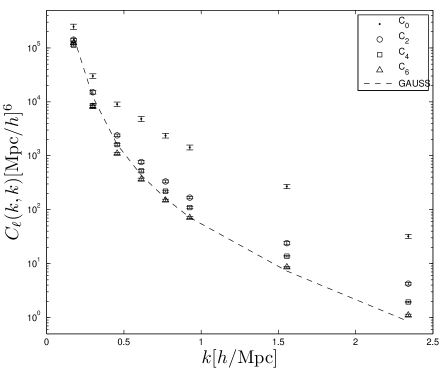
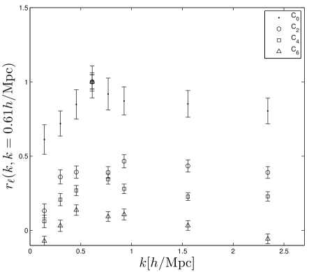
On the diagonal, the relative difference between the multipoles in the linear regime becomes smaller and converge to the predicted value, as expected. In addition, in the linear regime, the angular power of the off-diagonal elements (i.e. ) is one to two orders of magnitude smaller than the diagonal counter part. As we progress to the non-linear regime however, the off-diagonal elements decrease less rapidly, and a convenient way to express this is to look at the cross-correlation coefficient matrices.
6.4 matrices
As mentioned above, we need to look at an individual , for all scales combinations , and find the multipole beyond which the off-diagonal elements become negligible. The whole purpose behind this is to model the full covariance matrix as:
| (44) |
where the lower terms are measured from our simulations, and the others obtained from the Gaussian analytical prediction ([Eq.43]).
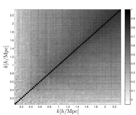
In the figures of this section, we present these ‘’ matrices, normalized to unity on the diagonal. These are thus in some sense equivalent to cross-correlation coefficient matrices. Fig. 12 presents the normalized matrix, which shows a structure similar to that of the cross-correlation coefficient matrices obtained previously (Fig. 7). The resemblance is not surprising, since , (we can see this by setting in [Eq. 40]) The matrix thus contains the information about the error bars of angle averaged power spectra, as well as their correlation.
By looking at the fractional error between the matrix and the actual covariance matrix of angle averaged power spectra (Fig. 13), we find that our method provides a very good agreement in the trans- and non-linear regimes, down to the few percent level. We do not show the largest scales, in which our method is more noisy, for reasons already explained. We recall that an extra contribution to , not included here, comes from the non-Gaussian Poisson uncertainty, as discussed in section 4.2, and needs to be included in the final analysis.
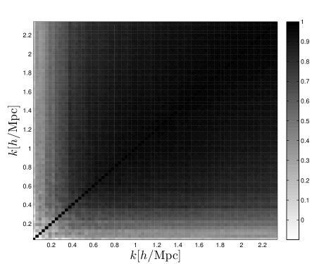
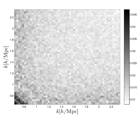
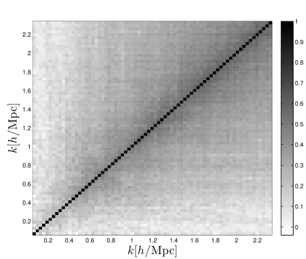
We now present the next few multipole matrices, and we found that beyond , very little information contained in the off-diagonal elements. Fig. 14 shows the matrix, again normalized to the diagonal for visual purposes. We observe that the smallest scales are correlated up to per cent. As discussed in sections 8.4 and 9, this matrix is a requirement for an accurate treatment of BAO and weak lensing data analyses, first because the uncertainties on the underlying galaxy surveys are not isothropic, and second because the optimal window function is often also angle-dependent Lu et al. (2010).
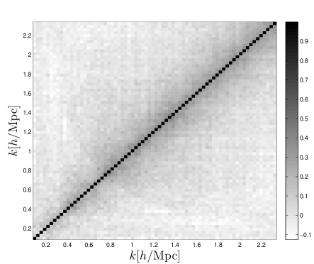
Fig. 15 shows that the correlation in the matrix is still of the order per cent for a good portion of the non-linear regime. The new feature here is that the strenght of the correlation of strongly non-linear modes among themselves starts to decrease as we move away from the diagonal. Fig. 16 shows that in , the matrix is mostly diagonal. As we progress through higher multipole moments, the off-diagonals become even dimmer, hence do not contain significant amount of new information. From this perspective, a multipole expansion up to is probably as far as one needs to push in order to medel correctly the off-diagonal elements.
Following [Eq.44], we thus propose to reconstruct the full from a combination of a) fully non-linear matrices (for ), presented above, b) analytical terms given by [Eq. 43] (which we scale up by per cent as mentioned in section 6.3), and c) non-Gaussian Poisson error, which depends solely on the number density od the sampled fields. In the next section, we decompose and simplify these matrices into a handfull of fitting functions, and show how one can easilly reconstruct the full at the percent level precision.
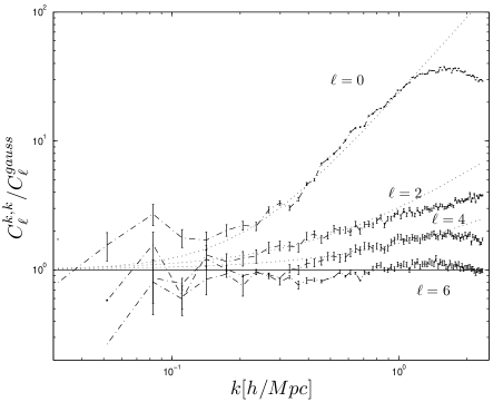
We next present in Fig. 17 the ratio of the diagonal of these matrices to the Gaussian prediction. We observe that all of them are consistent with the Gaussian prediction in the linear regime. As we progress towards the non-linear regime, the largest departure comes from the matrix, by a factor of about near . We observe a turn over at smaller scales, which is caused by our resolution limit. We opted not to model it in our fitting formula. and mildly break away from Gaussianity by factors of and at the same scale. All the higher ’s are consistent with Gaussian statistics. Over-plotted on the figure are fitting formulas, which are summarized in Table 1.
| 0 | 0.2095 | 1.9980 |
|---|---|---|
| 2 | 0.5481 | 0.7224 |
| 4 | 1.6025 | 1.0674 |
7 Factorization of the Matrices
In this section, we simplify even further our results with an Eigenvalue decomposition of the matrices, normalized to unity on their diagonal, as shown in the figures of section 6.4. We perform an iterative process to factorize each matrix into a purely diagonal component and a symmetric, relatively smooth off-diagonal part. The later can be further decomposed into a small set of Eigenvectors , corresponding to the largest Eigenvalues . These are then fitted with simple formulas. Combined with Gaussian predictions and fitting formulas from the deviation on the diagonal, one can fully reconstruct each of the matrix, and thus recover as well.
We start off the iteration by assigning the identity matrix to the diagonal component, which we subtract from the original matrix. We then extract from the remainder the principal Eigenvectors and recompose an new matrix as
| (45) |
For the next iteration, we model the diagonal as , and decompose the remainder once again. We iterate until the results converge, which takes about 4 steps. We vary the number of Eigenvalues we keep in our iteration, and keep the minimal number for which the reconstruction converges. In the end, the matrix is modeled as:
| (46) |
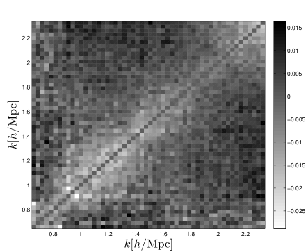
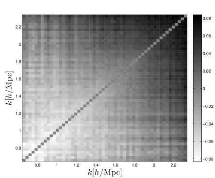
We show in Fig. 18 the fractional error between the original matrix and the factorized one. The factorization of the matrix with one Eigenvector reproduces the original matrix at the few percent level. The same procedure is also applied for the higher multipoles, in which we have included the first four Eigenmodes, and we find that the fractional error between the reconstructed and the original matrix are also of the order of a few percent.
We next fit these Eigenvectors with simple functions: for all ’s, the first Eigenvector is parametrized as , and all the other vectors as . The values of for the lowest three ’s are presented in Table 2. We required that all of these formulas vanish as , since the matrices become diagonal in the linear regime. The Eigenvectors of the matrix are presented in Fig. 20; over-plotted are the fitting formulas. The pixel-by-pixel agreement between the original matrices and those obtained from the fitted formulas is with less than 10 percent for all and .
Larger scales fluctuate much more as they are less accurately measured, hence the pixel-by-pixel agreement is not expected there. In addition, the matrices with are much harder to express with a small set of Eigenvectors, since the Eigenvalues are not decreasing fast enough. In any case, the first three harmonics we provide here contain most likely all the information one will ever use in realistic surveys and forecasts.
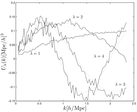
| 0 | 61.9058 | 0.0501 | 0.0207 | 0.6614 | 2.3045 |
|---|---|---|---|---|---|
| 2 | 35.7400 | 0.273 | 0.8266 | 1.962 | 0.816 |
| 4.4144 | 0.15772 | 2.4207 | 0.79153 | 0.032207 | |
| 1.7198 | 0.14426 | 4.0613 | 0.76611 | -0.26272 | |
| 0.9997 | 0.14414 | 5.422 | 0.84826 | 0.31324 | |
| 4 | 22.0881 | 0.060399 | 0.10344 | 0.64008 | 2.2584 |
| 4.5984 | 0.1553 | 2.3370 | 0.9307 | -0.1154 | |
| 2.2025 | 0.1569 | 3.6937 | 0.92304 | 0.04006 | |
| 1.4062 | 0.15233 | 5.1617 | 0.8899 | -0.14503 |
7.1 Non-Gaussian Poisson noise
The non-Gaussian Poisson uncertainty, whose construction was presented in section 4.2, can conveniently be incorporated in an analysis by finding the corresponding Eigenvalue and Eigenvectors of . Higher multipoles are not relevant as the angular distribution is flat, as shown in the middle plot of Fig. 2. We tested three number densities, corresponding to and . In all cases, we computed the covariance matrix, decomposed into a diagonal component and a cross-correlation coefficient matrix, found the matrix’s leading eigenvalue and Eigenvector, then fitted the latter with the same fitting function: . The diagonal was also fitted with a simple power law of the form
| (47) |
where . The best-fitting parameters are summarized in Table 3, and the performance of the Eigenvector fit can be found in the Appendix.
| 52.02 | 1.0193 | 0.0947 | 2.1021 | 2.5861 | 2.6936 | 2.1347 |
| 45.09 | 0.9987 | 0.2034 | 2.1553 | 2.3407 | 1.6533 | 2.1965 |
| 24.41 | 0.2966 | 3.3736 | 0.6099 | 0.6255 | -0.4321 | 2.0347 |
7.2 Recipe
Here we summarize our method to generate accurate non-Gaussian matrices. The full matrix is then given by [Eq. 44], where the terms are obtained from the fitting functions, and the higher multipole moments are obtained directly from [Eq. 43]. The sum over these Gaussian terms can be evaluated analytically as
| (48) | |||||
For the non-Gaussian terms, we proceed as follow: Each of the matrices, normalized on the diagonal, can be constructed from the first set of fit functions provided in Table 2, by following [Eq. 46]. The ‘un-normalized’ terms are then constructed by inverting [Eq. 32], where the diagonal elements are obtained from the product of the , also summarized in Table 2, with the Gaussian prediction [Eq. 43]. In other words:
| (49) | |||||
The complete covariance matrix is given by:
| (50) | |||||
with . This can be written in a more compact form as
| (51) | |||||
with
| (52) |
| (53) |
and
| (54) |
We conclude this section with a word of caution when using the fitting formulas provided here, in the sense that the range of validity of the fit has not been tested on other cosmological volumes. Consequently, we advice that one should limits itself to .
8 Measuring the Impact with Selection Functions
This section serves as a toy model for a realistic non-Gaussian error analysis, as it incorporates the non-Gaussian covariance matrix measured from N-body simulations with the 2dFGRS selection function (Norberg et al., 2002). We compare the estimated error bars on between the naive, purely diagonal, Gaussian covariance matrix, the effect of the one dimensional window function as prescribed by the FKP formalism, the unconvolved non-Gaussian covariance as measured from our N-body simulations, and the convolved non-Gaussian matrix.
We recall that in a periodic volume, a selection function that is exactly uniform throughout the volumes makes the observed and true covariance matrices exactly equal. That is only true in simulated volumes, and in that case, the optimal estimator for the power spectrum covariance matrix is obtained from the non-Gaussian covariance matrix directly measured from the simulations.
Non-periodicity is best dealt with by zero-padding the observed survey, which results in some coupling between different measure power spectrum bands. The coupling becomes more important as the selection function departs from a top hat, and in that case, the best estimator of the observed covariance matrix is a convolution of the 6-dimensional covariance over both vectors , given by:
| (55) |
The denominator is straight forward to calculate, while the numerator is a 6-dimensional integral, which must be calculated at all of the 6-dimensional coordinates, a task is computationally impossible to perform. For example, assuming that the size of the grid is cells, then for each pair, we have to sum over terms. We also have such pairs, and each term takes about flop. For , this process would take flop, and current supercomputers are in the regime of resolving flop per seconds. The above calculation would therefore take about 3000 years to complete. With the factorization proposed in this work however, it is now possible to break down the computation into smaller pieces and reduce the loops to 7 dimensions at most.
8.1 Factorization of the 6-dimensional covariance matrix
We propose here a break down of the true covariance matrix into a product of simple functions of the form , and where the angular components come exclusively from the Legendre polynomials. As explained in section 2.3, the argument of the Legendre polynomials, , is the (cosine of ) angle between and , which must first be expressed in terms of , following [Eq. 14]555In this section, we use instead of to denoted the (cosine of the) angle between the two Fourier modes, to avoid confusion with and , which corresponds to the angle of with respect to the -axis.. The only multipoles that appear in our equations are , so is to be expanded at most up to the fourth power. For a full factorization, the terms including must further be re-casted in their exponential form with Euler’s formula.
When computing the convolution, the first term on the right hand side of [Eq.51] is spherically symmetric, hence it must be convolved with the selection function as:
| (56) |
which is pretty much the FKP prescription, namely that the selection function is the only cause of mode coupling.
When computing the other terms of [Eq.51], which are the non-Gaussian contributions, we use the fact that the only coupling between the and vectors comes from the delta function, which couples their radial components. This means that all the angular integrations can be precomputed and stored in memory. For example, the only angular dependence in the multipole comes from the selection function itself, hence we can precompute
| (57) |
and the convolution is now four dimension smaller. The weight function is equal to unity for the term, and the comes in from the Jacobian in angular integration. For the higher multipoles, more of such terms must be precomputed as well, whose weight functions are summarized in Table 4.
8.2 The 2dFGRS selection function
The 2dFGRS(Colless et al., 2003) is comprised of two major regions, the NGP and the SGP, each of which take the overall form of a fan of degrees, extending from to . The selection function is constructed by first integrating the luminosity function over all the observed luminosity range, which is both redshift and angle dependent, and multiplying the result by the redshift completion function . Namely, we define the galaxy number density as:
| (58) |
where , being the characteristic galaxy luminosity, and given by
| (59) |
The three parameters , and are obtained from the 2dFGRS as , and respectively. The integral over gives an incomplete gamma function:
| (60) |
in which the term can be expressed as
| (61) | |||||
where is the angular dependence of the magnitude sensitivity, is the luminosity distance that is used to convert between absolute relative magnitudes, and the last term in the right hand side is the and corrections. Finally, the selection function is simply :
| (62) |
Both and are publicly available from the 2dFGRS website666www.mso.anu.edu.au/2dFGRS/. It is possible to obtain an even more accurate selection function by taking into account the redshift dependence of the magnitude sensitivity, however we do not need such an accuracy for the current work. We finally normalize the selection function such that
| (63) |
To understand the impact of the non-Gaussian Poisson uncertainty on the measured uncertainty, we test various templates, keeping the 2dFGRS selection function fixed. We follow the procedure of section 4.2, with an average number density of , which corresponds to an early data release of the 2dFGRS data. The final release contains more objects, and has a density of about . By comparison, the Poisson uncertainty corresponding to the number count of the Wiggle-Z survey could be modeled with for partial data and about for the final data release. We thus opt for two more number densities: and .
8.3 Results
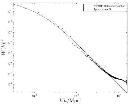
We assign the selection function on to a 256x256x128 grid, where the lower resolution is along the direction perpendicular from the NGP. We precompute the Fourier transform, and square each terms. Fig. 21 shows a comparison between the angle average of and a fitting function provided by the 2dFGRS group.
We then define a second set of bins in spherical coordinates, over which we perform the convolution. For that purpose, we divide the original volume of the survey into 64 radial bins, 48 polar bins and 32 azimuthal bins. The selection function is assigned in the grid by averaging over the 27 closest cells in the original grid. We have included a terms in each integrals over the polar angle, and a in each radial integral to properly account for the Jacobian matrix in spherical coordinates.
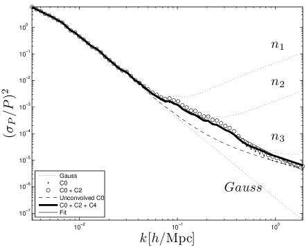
Fig. 22 shows the diagonal of the convolved covariance matrix, divided by , for the FKP prescription and for the progressive inclusion of and multipoles. Also overploted is the non-Gaussian results without the convolution. We see that already at , the non-Gaussian fractional error, after the convolution, deviates from the FKP prescription by a factor of about 3.0, while the unconvolved still traces quite well the FKP curve. This means that the mode mixing caused by the convolution with the survey selection function increases significantly the variance of the observed power spectrum. The departure gets amplified as one progresses towards higher modes, and by , the unconvolved departs from the FKP prescription by almost two orders of magnitudes. Interestingly, the convolved merges with the unconvolved counterpart at , where the BAO scale is usually cut off. inclusion of higher multipole increases the variance by a factor of about 2.0.
We have overplotted a simple smooth fitting function of the form :
| (64) |
which approximates the contribution from the three lower multipoles.
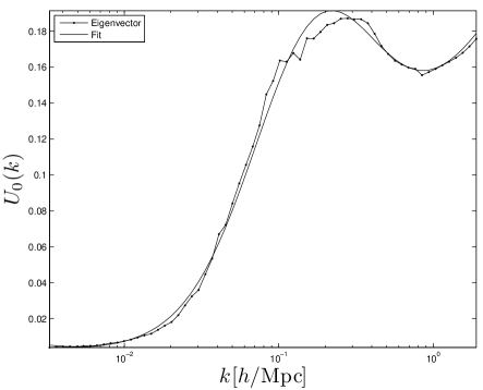
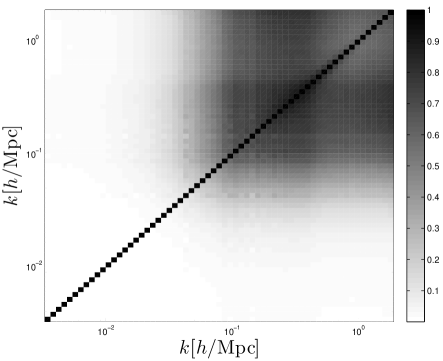
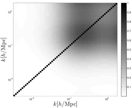
Fig. 24 shows the convolved cross-correlation coefficient matrix, where the angle average has been taken after the convolution. It is also possible to factorize this matrix, hence we proceed to an Eigenvalue decomposition, following the same iterative procedure as in section 7, solving for the first Eigenvector only. The Eigenvalue was found to be , and we used the sum of a quadratic and a Gaussian function to model the Eigenvector:
with and respectively. A comparison of the fit and the actual vector is presented in Fig. 23. The noise reduced cross-correlation coefficient matrix is presented in Fig. 25. We observe that the Fourier modes are already more than per cent correlated at , an significant enhancement compared to the unconvolved matrix, in which the equivalent coupling occurs roughly towards . This would most likely have an impact on a non-Gaussian BAO analysis.
8.4 Applications to weak lensing
The results presented in section 6.4 and the recipe presented in the previous section can find useful applications in the field of weak lensing. Convergence maps, for instance, are constructed from a redshift integral over a past line cone filled with dark matter, weighted by a geometric kernel. Because of the projection nature of this process, the survey maps are sensitive to both large and small scales, where non-Gaussianities have been observed in the convergence power spectrum (Doré et al., 2009).
It has recently been demonstrated that weak lensing of high redshift sources by large scale structures can serve as a probe of the dark energy equation of state (Huterer, 2002). To make a complex story short, the weak lensing power spectrum is closely related to that of the three dimensional dark matter via Limber’s approximation (Limber, 1954), hence it is similarly sensitive to cosmological parameters. It was then realized that the same structures were also distorting the signal of high redshift source of 21 cm emission (Metcalf & White, 2009), hence the detection of weak lensing from diffuse temperature fields could also constrain the dark energy. The lensing fields are quadratic functions of smoothed temperature fields, and the optimal smoothing window function depends not only on the the parameter under study, but also on the statistical nature of the source and lenses (Lu & Pen, 2008).
Optimal quadratic estimators of lensing fields were first obtained under the Gaussian assumption (Hu & Okamoto, 2002; Zahn & Zaldarriaga, 2006), but it was soon realized that when the observed field is non-Gaussian, the proposed estimators are no longer optimal: the noise estimation can be underestimated by several orders of magnitude (Lu & Pen, 2008). Optimal non-Gaussian lensing estimators were then obtained from N-body simulations (Lu et al., 2010), and it was found that the optimal smoothing window function for dark energy involves the first two multipoles of the dark matter power spectrum covariance matrix, and (see [Eqs. ] in (Lu et al., 2010)). The tools developed in the present paper thus allow one to construct, for the first time and from simple fitting functions, optimal non-Gaussian estimators of dark energy parameters from 21 cm temperature maps.
The survey selection function was factored out of the above discussion, which was interested solely in the non-Gaussianities inherent in the sources and lenses. However, cosmology from weak lensing observations of galaxy and quasar surveys is affected by selection functions, in a similar way to BAO analyses discussed in this paper: the underlying 2- and 4-point functions in Fourier space are inevitably convolved with the survey selection function. With the factorization proposed in the paper, this convolution should also be relatively simple to perform, and allows one to measure non-Gaussian error bars on the lensing power spectrum, which includes the effect of the non-linear dynamics, of the selection function, and possibly of Poisson noise.
In particular, the weak lensing convergence field is obtained from the dark matter field from
| (66) |
with
| (67) |
is the Hubble parameter, the speed of light, and the comoving distances to the lenses and to the source respectively. When one has knowledge of the three dimensional selection function, it can be incorporated in the above equation as
| (68) |
we can be further compactified if one absorbs in the definition of the selection function. The result takes the form of an integral over one dimension of an observed density fields: . This means that all the non-Gaussian calculations performed on the three dimensional density fields (i.e. see section 2.3) can be extended to weak lensing maps by the simple modification of the selection function mentioned above, plus an integration over the third dimension (in the small angle approximation at least). In particular, the best estimate of the non-Gaussian lensing covariance matrix is obtained from solving [Eq. 13] with the modified selection function, then by integrating the two -components with, at each integration step, the inclusion of an extra weight for the conversion of -modes to -modes.
9 Discussion
We have found that even for modes of , the non-Gaussian error bars are higher than those prescribed by the FKP method by a factor of a few, due to mode coupling caused by the convolution of the selection function. This has to be put in contrast with results from pure N-body simulations, which show that the departure from Gaussianity reaches this sort of amplitudes at higher -modes, as seen from Fig. 22. We also observe that with the 2dFGRS, the non-Gaussian Poisson noise plays an important role if the number density is smaller than , but is not enough to characterize all of the non-Gaussian features of the density field. The term is the leading contribution of the enhancement observed in the range , but for larger -modes, and both play an important role.
Without the convolution, keeping only the term, and assuming that the BAO measurement was performed with a non-Gaussian estimator, the propagation of the non-Gaussianities on to the BAO dilation scale produces very similar constraints (Takahashi et al., 2011). The estimators that are used in the data analyses however are Gaussian, while the power spectrum covariance matrices that enter the calculations are either Gaussian or obtained with mock catalogs. As pointed out previously (Ngan et al., 2011), the estimators constructed in such a way are inconsistent and should be noise weighted. When correcting for that effect, it was found that the consistent – but suboptimal – error bars are about per cent higher than those obtained assuming an optimal estimator. In the light of the current results, the observed (i.e. convolved) covariance matrix is even less Gaussian, and it is not obvious that the error on the BAO dilation scale will be unaffected by this new estimates, since our measurement show significant deviations at scales as large as .
It is worth mentioning again that the measurement of the from provides an alternative way to extract the covariance matrix of the angle average power spectra. Although the mean value of both methods is identical, i.e. unbiased, the second gives us a better handle on the error on each matrix element, hence provide an optimal measurement of their uncertainty. We have shown in this paper that each matrix element receives its dominant contribution from small angles, while larger angles are more noisy. It is thus in possible to re-weight the sum by taking this new information into account, and obtain more accurate error bars on each matrix element, compared to the current bootstrap method (HDP2). As mentioned in the introduction, our next objective is to achieve a similar accuracy with a much lower number of simulations. This would revolutionize the field of observational cosmology as the covariance matrix would be measured internally, i.e. directly from the data.
The techniques presented in this paper call for extensions, as we did not include redshift distortions nor shot noise in our analysis. The latter will become important when repeating this procedure on haloes, and it was shown (Neyrinck et al., 2006) that the Fisher information in haloes is also departing from Gaussianity. It is straight forward to perform a similar analyses with a quadratic halo model, where the halo density is parametrized by . This involves an extra cross correlation between the linear and quadratic term, and leaves some room for the choice of and , and ultimately, one should work straight from a halo catalog. The optimal estimator should also be based on a cosmology independent model of the covariance matrix, hence one should compute how the fitting functions scale with and .
As mentioned earlier, the effect of the selection functions is enhanced for survey geometries that are different from top-hats, and it would be interesting to repeat some of the BAO data analyses that were performed on such surveys, like the 2dFGRS, Wiggle-Z. The current method also applies to surveys with irregular geometries like those obtained from the Lyman- forest (McDonald & Eisenstein, 2007; McQuinn & White, 2011), and we are hoping that it will considered in the elaboration of these future analysis pipelines.
We leave it for future work to match our results with predictions from higher order perturbation theory. We would like to verify that the angular dependence we observe in the covariance matrix is predicted by a complete 4-points function analysis, at least in the trans-linear regime. In addition, the extraction of non-Gaussian error bars from two dimensional angular clustering could also be performed with techniques similar to those employed here.
10 Conclusion
Estimating accurately the non-linear covariance matrix of the matter power spectrum is essential when constraining cosmological parameters including, but not restricted to, the dark energy equation of state . So far, many BAO analyses from galaxy surveys were performed under the assumption that the underlying density field is Gaussian, which yields a suboptimal measurement of the mean power spectrum (and thus of the BAO dilation scale), and, at least as important, the error bars are biased.
To estimate unbiased error bars on the dilation scale is a challenging task but can now be done. In the simple case of periodic volume, it was shown recently (Ngan et al., 2011) that, first, an unbiased error bar on a suboptimal measurement of the mean could be obtained from the knowledge of the underlying covariance matrix. Second, if one did measure optimally the mean BAO dilation scale, then the optimal measurement of the error requires an estimate of the inverse of the power spectrum covariance matrix. This is much more challenging due to the presence of noise, even when dealing with simulations embedded in periodic volumes, but improves the constraining performance by a significant amount.
When estimating the power spectrum and its uncertainty from data, the survey selection function complicates the calculations since the observed quantities are actually convolved with the selection function. Since the covariance matrix is not isotropic, as it depends on the relative angle between two Fourier modes, the convolution cannot be simply factored into two radial components. Hence we are left with a challenging six-dimensional integral to perform, which so far has been an unresolved problem.
In this paper, we present a method to perform this convolution for an arbitrary galaxy survey selection function, that thus allows one to measure unbiased error bars on the matter power spectrum. The estimate is still suboptimal, unless one combines our tools with the PKL formalism, but we have nevertheless removed the bias on the error bar.
From an ensemble of 200 N-body simulations, we have measured the angular dependence of the covariance of the matter density power spectrum. We have found that on large scales, there is only a weak dependence, consistent with the Gaussian aspect of the fields in that regime. On smaller scales, however, we have detected a strong signal coming from Fourier modes separated by small angles. This comes from the fact that the complex phases of these modes are similar, hence they tend to couple first. We next expanded the covariance into a multipole series, and found that only the first three even poles were significantly different from Gaussian fields.
We further decomposed these matrices into diagonal terms and cross-correlation coefficient matrices, from which we extracted the principal Eigenvectors. This allowed us to break down the underlying six-dimensional covariance into a set of Eigenvectors, Eigenvalues and three diagonals terms. We provided simple fitting formulas for each of these quantities, and thus enable one to construct a full six-dimensional covariance matrix with an accuracy at the few per cent level.
Intrinsically, non-Gaussianities introduce matrix elements to be measured in N-body simulations, as opposed to for Gaussian fields. With the proposed method, the number of parameters to measure is reduced to a handful, even if the survey selection function is non-trivial. This opens up the possibility to measure non-Gaussianities directly from the data, which we will investigate in part II of our work.
This factorization is necessary in order to estimate unbiased non-Gaussian error bars on a realistic galaxy survey, that must include the effect of the survey selection function. We found that in the case of the 2dFGRS selection function, the non-Gaussian fractional variance at is larger by a factor of three compared to the estimate from the FKP prescription, and more than an order of magnitude at . With similar techniques, we were able to propagate a few templates of non-Gaussian Poisson error matrices into the convolution and estimate the impact on the measured power spectrum. We showed that with the 2dFGRS selection function, the non-Gaussian Poisson noise corresponding to a number density significantly lower than has a large effect on the fractional variance at scales relevant for BAO analyses and should be incorporated in an unbiased analysis. The cross-correlation coefficient matrix of the convolved power spectrum shows that the correlation propagates to larger scales in the convolution process, and should have a larger impact on BAO analyses for instance. We conclude by emphasizing on the fact that constraints on cosmological parameters obtained from BAO analyses of galaxy surveys are currently significantly biased and suboptimal, but that both of these effects can now be dealt with in further analyses.
Acknowledgments
The authors would like to thank Olivier Doré, Ilana MacDonald and Patrick McDonald for useful discussions, Daniel Eisenstein, Martin White and Chris Blake for their comments on early versions of the manuscript, and to acknowledge the financial support provided by NSERC and FQRNT. The simulations and computations were performed on the Sunnyvale cluster at CITA. We also acknowledge the 2dFGRS mask software written by Peder Norberg and Shaun Cole.
Appendix A Normalization
We present in this appendix the interpretation of the normalization of the angular covariance (see [Eq. 26 and 27]). The shape of this function is plotted in Fig. 26, for a scale that corresponds to , which lies close to the transition between trans-linear and non-linear regime at .
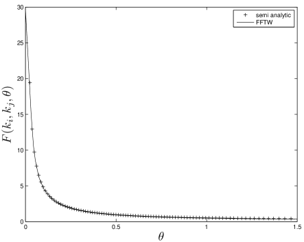
In fact, the normalization is simply a counting of the different combinations of that produce a given . We see from the figure that at small angles (i.e. small ), there is a lot of possible combinations, and that the function rapidly decreases with the angle. To capture this, imagine counting the number of times we can embed both ends of a given vector on a given spherical shell. In the thin shell approximation and for a vector with non-zero length, the vector can be moved around an axis parallel to the vector, that also passes through the centre of the shell. In terms of solid geometry, the vector spans the flat side of a cylinder that intersects the shell. The normalization is proportional to the circumference of the cylinder’s basis, and as the length of the vector decreases, so does the height of the cylinder, hence its circumference increases. In the discrete case, the shells have a finite thickness, and are constructed out of a grid. The normalization thus produces integer counts, which discretizes the subtended angles.
Appendix B Legendre-Gauss Weighted Summation
The conversion of the integral into a sum is performed using a Legendre-Gauss weighted sum(Abbott, 2005), in which ‘colocation’ knots, which we label with , are placed at the zeros of the Legendre polynomial . We choose , and we exclude the end points at in order to isolate the zero-lag contribution. The weights are given by:
| (69) |
This Gaussian quadrature gives an exact representation of the integral for polynomials of degree or less, and provides a pretty good fit to most of our . In the linear regime, the discretization effect becomes important, and the number of angles one can make between the grid cells drops down as . In the case were fewer points are available, we choose = , , or depending on the number of available angular bins. Once we have specified the knots, then, for each scale combination, we interpolate the angular covariance on to these knots, and then perform the weighted sum. As mentioned above, we always treat the zero-lag point separately in order to avoid interpolating its value to the nearest neighbors. We thus break the summation in two pieces:
| (70) | |||||
The factor of comes from the integral over the angle, and is half the distance to the first knot.
Appendix C Eigenvector of the Poisson noise
This Appendix presents the Eigenvector that best describes the non-Gaussian Poisson noise, as discussed in section 7.1. We restrict ourselves with the case where the number density is the highest, even though similar analyses can be carried for the other values of we studied in this paper. We present in Fig. 27 the Eigenvector itself, compared to the best-fitting formula provided. We next compare the covariance matrix constructed from the fitting functions with the original, and present the fractional error in Fig. 28, which shows a few per cent agreement. When compared with the predictions from (Cohn, 2006), we observe that the overall trends are consistent: first, the Gaussian contribution to the error decreases as one probes smaller scales. Second, densities with lower see their Gaussian contribution being reduced in the trans-linear regime, where the non-Gaussian Poisson counting becomes more important. Third, densities with lower produce larger cross-correlation coefficients of tran-linear scales, also in accordance with the predictions.
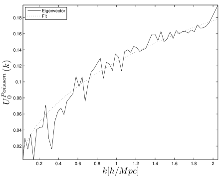
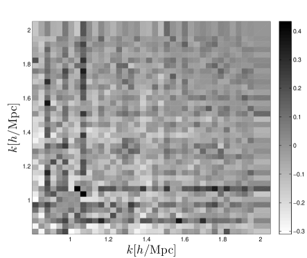
References
- Abbott (2005) Abbott P., 2005, Mathematica J, 9, 689
- Acquaviva et al. (2008) Acquaviva V., Hajian A., Spergel D. N., Das S., 2008, Phys. Rev. D, 78, 043514
- Albrecht et al. (2006) Albrecht A., et al., 2006, ArXiv e-prints (astro-ph/060959)
- Beaulieu et al. (2010) Beaulieu J. P., et al., 2010, in V. Coudé Du Foresto, D. M. Gelino, & I. Ribas ed., Pathways Towards Habitable Planets Vol. 430 of Astronomical Society of the Pacific Conference Series, EUCLID: Dark Universe Probe and Microlensing Planet Hunter. pp 266–+
- Benítez et al. (2009) Benítez N., et al., 2009, ApJ, 691, 241
- Bernardeau et al. (2002) Bernardeau F., Colombi S., Gaztañaga E., Scoccimarro R., 2002, Phys. Rep., 367, 1
- Blake et al. (2010) Blake C., et al., 2010, MNRAS, 406, 803
- Blake et al. (2011) Blake C., et al., 2011, ArXiv e-prints (astro-ph/1105.2862)
- Chiang et al. (2002) Chiang L.-Y., Coles P., Naselsky P., 2002, MNRAS, 337, 488
- Cohn (2006) Cohn J. D., 2006, New Astronomy, 11, 226
- Cole et al. (2005) Cole S., et al., 2005, MNRAS, 362, 505
- Coles & Chiang (2000) Coles P., Chiang L., 2000, Nature, 406, 376
- Colless et al. (2003) Colless M., et al., 2003, ArXiv e-prints (astro-ph/0306581)
- Doré et al. (2009) Doré O., Lu T., Pen U.-L., 2009, ArXiv e-prints
- Drinkwater et al. (2010) Drinkwater M. J., et al., 2010, MNRAS, 401, 1429
- Eisenstein et al. (2005) Eisenstein D. J., et al., 2005, ApJ, 633, 560
- Feldman et al. (1994) Feldman H. A., Kaiser N., Peacock J. A., 1994, ApJ, 426, 23
- Hu & Okamoto (2002) Hu W., Okamoto T., 2002, ApJ, 574, 566
- Huchra et al. (1990) Huchra J. P., Geller M. J., de Lapparent V., Corwin Jr. H. G., 1990, ApJS, 72, 433
- Huterer (2002) Huterer D., 2002, Phys. Rev. D, 65, 063001
- Hütsi (2006) Hütsi G., 2006, A&A, 449, 891
- Jing (2005) Jing Y. P., 2005, ApJ, 620, 559
- Lazio (2008) Lazio J., 2008, in R. Minchin & E. Momjian ed., The Evolution of Galaxies Through the Neutral Hydrogen Window Vol. 1035 of American Institute of Physics Conference Series, The Square Kilometer Array. pp 303–309
- Limber (1954) Limber D. N., 1954, ApJ, 119, 655
- LSST Science Collaborations et al. (2009) LSST Science Collaborations et al., 2009, ArXiv e-prints (astro-ph/0912.0201)
- Lu & Pen (2008) Lu T., Pen U.-L., 2008, MNRAS, 388, 1819
- Lu et al. (2010) Lu T., Pen U.-L., Doré O., 2010, Phys. Rev. D, 81, 123015
- McDonald & Eisenstein (2007) McDonald P., Eisenstein D. J., 2007, Phys. Rev. D, 76, 063009
- McQuinn & White (2011) McQuinn M., White M., 2011, MNRAS, 415, 2257
- Meiksin & White (1999) Meiksin A., White M., 1999, MNRAS, 308, 1179
- Merz et al. (2005) Merz H., Pen U.-L., Trac H., 2005, New Astronomy, 10, 393
- Metcalf & White (2009) Metcalf R. B., White S. D. M., 2009, MNRAS, 394, 704
- Neyrinck et al. (2006) Neyrinck M. C., Szapudi I., Rimes C. D., 2006, MNRAS, 370, L66
- Ngan et al. (2011) Ngan W.-H. W., Harnois-Déraps J., Pen U.-L., McDonald P., MacDonald I., 2011, ArXiv e-prints (astro-ph/1106.5548)
- Norberg et al. (2002) Norberg P., et al., 2002, MNRAS, 336, 907
- Percival et al. (2007) Percival W. J., Cole S., Eisenstein D. J., Nichol R. C., Peacock J. A., Pope A. C., Szalay A. S., 2007, MNRAS, 381, 1053
- Percival et al. (2001) Percival W. J., et al., 2001, MNRAS, 327, 1297
- Peterson et al. (2006) Peterson J. B., Bandura K., Pen U. L., 2006, ArXiv e-prints (astro-ph/0606104)
- Rimes & Hamilton (2005) Rimes C. D., Hamilton A. J. S., 2005, MNRAS, 360, L82
- Sato et al. (2011) Sato T., Hütsi G., Yamamoto K., 2011, Progress of Theoretical Physics, 125, 187
- Schlegel et al. (2009) Schlegel D., White M., Eisenstein D., 2009, ArXiv e-prints (astro-ph/0902.4680)
- Seljak & Zaldarriaga (1996) Seljak U., Zaldarriaga M., 1996, ApJ, 469, 437
- Takahashi et al. (2009) Takahashi R., et al., 2009, ApJ, 700, 479
- Takahashi et al. (2011) Takahashi R., et al., 2011, ApJ, 726, 7
- Tegmark (1997) Tegmark M., 1997, Phys. Rev. Lett., 79, 3806
- Tegmark et al. (2006) Tegmark M., et al., 2006, Phys. Rev. D, 74, 123507
- Vogeley & Szalay (1996) Vogeley M. S., Szalay A. S., 1996, ApJ, 465, 34
- York et al. (2000) York D. G., et al., 2000, AJ, 120, 1579
- Zahn & Zaldarriaga (2006) Zahn O., Zaldarriaga M., 2006, ApJ, 653, 922