Ideal chains with fixed self-intersection rate

Simone Franchini Dipartimento di Fisica, Sapienza UniversitΓ  di Roma, Piazzale A. Moro 2, I-00185 Roma, Italy simone.franchini@yahoo.it
Abstract

We consider ideal chains in a hypercubic lattice β„€dsuperscript℀𝑑\mathbb{Z}^{d}, dβ‰₯3𝑑3d\geq 3, with a fixed ratio mπ‘šm of self-intersection per monomer. Despite the simplicity of the geometrical constraint, this model shows some interesting properties, such as a collapse transition for a critical value mcsubscriptπ‘šπ‘m_{c}. Numerical simulations show a Self-Avoiding-Walk-like behavior for m<mcπ‘šsubscriptπ‘šπ‘m<m_{c}, and a compact cluster configuration for m>mcπ‘šsubscriptπ‘šπ‘m>m_{c}. The collapse seems to show the same characteristics as the canonical thermodynamical models for the coil-globule transition.

Random Walks, Ideal Polymers, Ideal Chains, Coil-Globule Transition
pacs:
05.40.Fb, 05.70.Fh

I Introduction

Polymer models have been the subject of extensive theoretical and numerical studies. Most of these models are based on ideal flexible chains, with the addition of various kinds of interactions between monomers, to include some non-trivial properties of real systems des Cloizeaux ; De Gennes-Scal. .

Very important is the excluded volume effect, which significantly modifies the fractal properties (the chains behave like Self-Avoiding Walks, SAW); and the coil-globule (CG) transition, in which a flexible chain collapses from an extended coil to a liquid-like globule De Gennes-Scal. ; Grosberg-Kuznestov .

Most of the thermodynamic models that show the CG transition usually consider a competition between interactions of different geometrical nature. For instance, one can consider a lattice random chain with repulsive on-site interactions and attractive nearest-neighbors links. The transition arises from the competition of these interactions.

Let Ο‰={S0,S1,…,Sn}πœ”subscript𝑆0subscript𝑆1…subscript𝑆𝑛\omega=\left\{S_{0},S_{1},\,...\,,S_{n}\right\} be an nβˆ’limit-from𝑛n-step Simple Random Walk (SRW) on the β„€dsuperscript℀𝑑\mathbb{Z}^{d} lattice (Sisubscript𝑆𝑖S_{i} are lattice vectors), and define the number of visits to each site xπ‘₯x as ψx=βˆ‘iδ​(xβˆ’Si)subscriptπœ“π‘₯subscript𝑖𝛿π‘₯subscript𝑆𝑖\psi_{x}=\sum_{i}\delta\left(x-S_{i}\right). A canonical model, incorporating excluded volume and a CG transition, is described by the Hamiltonian

ℋ​[ψ]=Ο΅0β€‹βˆ‘xψx2βˆ’Ο΅1β€‹βˆ‘βŸ¨x,y⟩ψxβ€‹Οˆy,β„‹delimited-[]πœ“subscriptitalic-Ο΅0subscriptπ‘₯superscriptsubscriptπœ“π‘₯2subscriptitalic-Ο΅1subscriptπ‘₯𝑦subscriptπœ“π‘₯subscriptπœ“π‘¦\mathcal{H}\left[\psi\right]=\epsilon_{0}\sum_{x}\psi_{x}^{2}-\epsilon_{1}\sum_{\langle x,y\rangle}\psi_{x}\psi_{y}, (1)

where ⟨x,y⟩π‘₯𝑦\langle x,y\rangle indicates nearest-neighbors (taking Ο΅1=0subscriptitalic-Ο΅10\epsilon_{1}=0 will lead to the Domb-Joyce model, see Huges ).

A few years ago an interesting thermodynamic model that shows a transition with only on-site interactions was proposed Krawckzyk . However, a competition between two geometrically different constraints is still present since a self-avoidance is incorporated through restricting the maximal number of visits per site.

To our knowledge all the thermodynamic models proposed so far, having only one kind of short-range interaction, do not allow for the CG transition in the Boltzmann parameter.

In this work we will show how excluded volume effects, the CG transition and liquid-like clusters can be obtained by imposing a single global geometric constraint. We consider ideal chains in a hypercubic lattice β„€dsuperscript℀𝑑\mathbb{Z}^{d}, dβ‰₯3𝑑3d\geq 3, with a fixed ratio mπ‘šm of self-intersections per monomer.

This model shows a CG transition for a critical ratio mcsubscriptπ‘šπ‘m_{c}: numerical simulations (obtained by a standard implementation of the Pruned-Enriched Rosenbluth Method, PERM, see PERM ; Grassberger ; Prellberg ; Hsu-Grassberger ) indicate a SAW-like behavior for m<mcπ‘šsubscriptπ‘šπ‘m<m_{c} (for a review about SAW see Madras-Slade ; Clisby ; Owczarek ) and a cluster configuration for m>mcπ‘šsubscriptπ‘šπ‘m>m_{c}. In addition the model is amongst the simplest with a crossover from SAW to cluster behaviour. Our focus will be on dβ‰₯3𝑑3d\geq 3 lattices because in these lattices, as we shall see, the transition occurs at non-trivial values of mcsubscriptπ‘šπ‘m_{c}.

II Model definition

Consider an ideal chain Ο‰πœ”\omega of n𝑛n steps on β„€dsuperscript℀𝑑\mathbb{Z}^{d} (without loss of generality we take S0=0subscript𝑆00S_{0}=0). We call R​[Ο‰]𝑅delimited-[]πœ”R\left[\omega\right] the range of Ο‰πœ”\omega (number of distinct lattice sites visited by the path), and M​[Ο‰]=(n+1)βˆ’R​[Ο‰]𝑀delimited-[]πœ”π‘›1𝑅delimited-[]πœ”M\left[\omega\right]=\left(n+1\right)-R\left[\omega\right] the number of self-intersections.

Let Pn​(M)subscript𝑃𝑛𝑀P_{n}\left(M\right) be the fraction of SRW, of length n𝑛n, with exactly M∈[0,nβˆ’1]𝑀0𝑛1M\in\left[0,n-1\right] self-intersections. We introduce mean value ⟨Mn⟩delimited-⟨⟩subscript𝑀𝑛\langle M_{n}\rangle and variance βŸ¨Ξ”β€‹Mn2⟩=⟨Mn2βŸ©βˆ’βŸ¨Mn⟩2delimited-βŸ¨βŸ©Ξ”superscriptsubscript𝑀𝑛2delimited-⟨⟩superscriptsubscript𝑀𝑛2superscriptdelimited-⟨⟩subscript𝑀𝑛2\langle\Delta M_{n}^{2}\rangle=\langle M_{n}^{2}\rangle-\langle M_{n}\rangle^{2} of the distribution Pn​(M)subscript𝑃𝑛𝑀P_{n}\left(M\right). It is well known (see Huges ) that for SRW in dβ‰₯3𝑑3d\geq 3, dβ‰ 4𝑑4d\neq 4,

⟨Mn⟩=Cd​nβˆ’Ξ”d​n2βˆ’d2+π’ͺ​(1),delimited-⟨⟩subscript𝑀𝑛subscript𝐢𝑑𝑛subscriptΔ𝑑superscript𝑛2𝑑2π’ͺ1\langle M_{n}\rangle=C_{d}n-\Delta_{d}n^{2-\frac{d}{2}}+\mathcal{O}\left(1\right), (2)

where Cdsubscript𝐢𝑑C_{d} is the probability that an infinite length walk contains its starting site at least twice (for numerical values of Cdsubscript𝐢𝑑C_{d}, see Douglas ), and Ξ”dsubscriptΔ𝑑\Delta_{d} is exactly known (for d=4𝑑4d=4 the main fluctuation is actually Ξ”4​log⁑(n)subscriptΞ”4𝑛\Delta_{4}\log\left(n\right)) Huges ; Douglas . Concerning the variance, Jain and Pruitt have shown that βŸ¨Ξ”β€‹Mn2⟩∝n​log⁑(n)proportional-todelimited-βŸ¨βŸ©Ξ”superscriptsubscript𝑀𝑛2𝑛𝑛\langle\Delta M_{n}^{2}\rangle\propto n\log\left(n\right) for d=3𝑑3d=3, and βŸ¨Ξ”β€‹Mn2⟩∝nproportional-todelimited-βŸ¨βŸ©Ξ”superscriptsubscript𝑀𝑛2𝑛\langle\Delta M_{n}^{2}\rangle\propto n for dβ‰₯4𝑑4d\geq 4 Huges ; Jain-Pruitt . They have also shown that for dβ‰₯2𝑑2d\geq 2

ΞΎ=limnβ†’βˆž(Mβˆ’βŸ¨Mn⟩)/βŸ¨Ξ”β€‹Mn2βŸ©πœ‰subscript→𝑛𝑀delimited-⟨⟩subscript𝑀𝑛delimited-βŸ¨βŸ©Ξ”superscriptsubscript𝑀𝑛2\xi=\lim_{n\rightarrow\infty}\left(M-\langle M_{n}\rangle\right)/\langle\Delta M_{n}^{2}\rangle (3)

is normally distributed, from which it follows that Pn​(M)subscript𝑃𝑛𝑀P_{n}\left(M\right) is peaked around its mean value for long walks.

We are interested in chains in which the rate of intersections per monomer is fixed at a certain value m∈[0,1]π‘š01m\in\left[0,1\right] in the thermodynamic limit. We define the ensemble Ξ©msubscriptΞ©π‘š\Omega_{m} of nβˆ’limit-from𝑛n-step walks with exactly M=⌊m​(nβˆ’1)βŒ‹π‘€π‘šπ‘›1M=\left\lfloor m\left(n-1\right)\right\rfloor intersections, and ΩΩ\Omega, the ensemble of all nβˆ’limit-from𝑛n-step SRW: we call βŸ¨β‹…βŸ©msubscriptdelimited-βŸ¨βŸ©β‹…π‘š\langle\cdot\rangle_{m} the average on Ξ©msubscriptΞ©π‘š\Omega_{m}, and βŸ¨β‹…βŸ©delimited-βŸ¨βŸ©β‹…\langle\cdot\rangle that of ΩΩ\Omega.

For large n𝑛n we can approximate ⌊m​(nβˆ’1)βŒ‹β‰ƒm​nsimilar-to-or-equalsπ‘šπ‘›1π‘šπ‘›\left\lfloor m\left(n-1\right)\right\rfloor\simeq mn. Henceforth we will work under this approximation. We introduce the fraction of mβˆ’limit-fromπ‘šm-intersection rate walks as Pn​(m)subscriptπ‘ƒπ‘›π‘šP_{n}\left(m\right). From the properties of Pn​(M)subscript𝑃𝑛𝑀P_{n}\left(M\right) it follows that Pn​(m)subscriptπ‘ƒπ‘›π‘šP_{n}\left(m\right) is peaked around ⟨m⟩=Cddelimited-βŸ¨βŸ©π‘šsubscript𝐢𝑑\langle m\rangle=C_{d} when nβ†’βˆžβ†’π‘›n\rightarrow\infty.

Let ⟨Sn2⟩msubscriptdelimited-⟨⟩superscriptsubscript𝑆𝑛2π‘š\langle S_{n}^{2}\rangle_{m} be the mean square end-to-end distance on Ξ©msubscriptΞ©π‘š\Omega_{m}: from our simulations we find that the relation ⟨Sn2⟩m∝n2​νd​(m)proportional-tosubscriptdelimited-⟨⟩superscriptsubscript𝑆𝑛2π‘šsuperscript𝑛2subscriptπœˆπ‘‘π‘š\langle S_{n}^{2}\rangle_{m}\propto n^{2\nu_{d}\left(m\right)} holds for any dimension considered, with the exponent Ξ½d​(m)subscriptπœˆπ‘‘π‘š\nu_{d}\left(m\right) dependent on mπ‘šm and d𝑑d. Again, for dβ‰₯3𝑑3d\geq 3, the simulations show the existence of a critical value mc∈(0, 1)subscriptπ‘šπ‘01m_{c}\in\left(0,\,1\right) beyond which the chains collapse into a compact liquid-like globule, with Ξ½d​(m)=1/dsubscriptπœˆπ‘‘π‘š1𝑑\nu_{d}\left(m\right)=1/d. If instead m<mcπ‘šsubscriptπ‘šπ‘m<m_{c} we have the SAW-like behavior (Fig. (1) and (2)). As preliminary observation we can state that, since for m=0π‘š0m=0 we have the Self-Avoiding Walk, then ⟨Sn2⟩0≃Dd​n2​νdsimilar-to-or-equalssubscriptdelimited-⟨⟩superscriptsubscript𝑆𝑛20subscript𝐷𝑑superscript𝑛2subscriptπœˆπ‘‘\langle S_{n}^{2}\rangle_{0}\simeq D_{d}n^{2\nu_{d}} (Ξ½dsubscriptπœˆπ‘‘\nu_{d} is the correlation length exponent for the SAW, see Madras-Slade ). On the other hand, from Eq. (3) it follows that the relation

βˆ«βˆ’bnbnπ‘‘Ο΅β€‹βŸ¨Sn2⟩Cd+ϡ​Pn​(Cd+Ο΅)≃n,similar-to-or-equalssuperscriptsubscriptsubscript𝑏𝑛subscript𝑏𝑛differential-ditalic-Ο΅subscriptdelimited-⟨⟩superscriptsubscript𝑆𝑛2subscript𝐢𝑑italic-Ο΅subscript𝑃𝑛subscript𝐢𝑑italic-ϡ𝑛\int_{-b_{n}}^{b_{n}}d\epsilon\,\langle S_{n}^{2}\rangle_{C_{d}+\epsilon}P_{n}\left(C_{d}+\epsilon\right)\simeq n, (4)

should hold in the large n𝑛n limit and bn=o​(1)subscriptπ‘π‘›π‘œ1b_{n}=o\left(1\right). This is clearly confirmed by our simulations.
Refer to caption
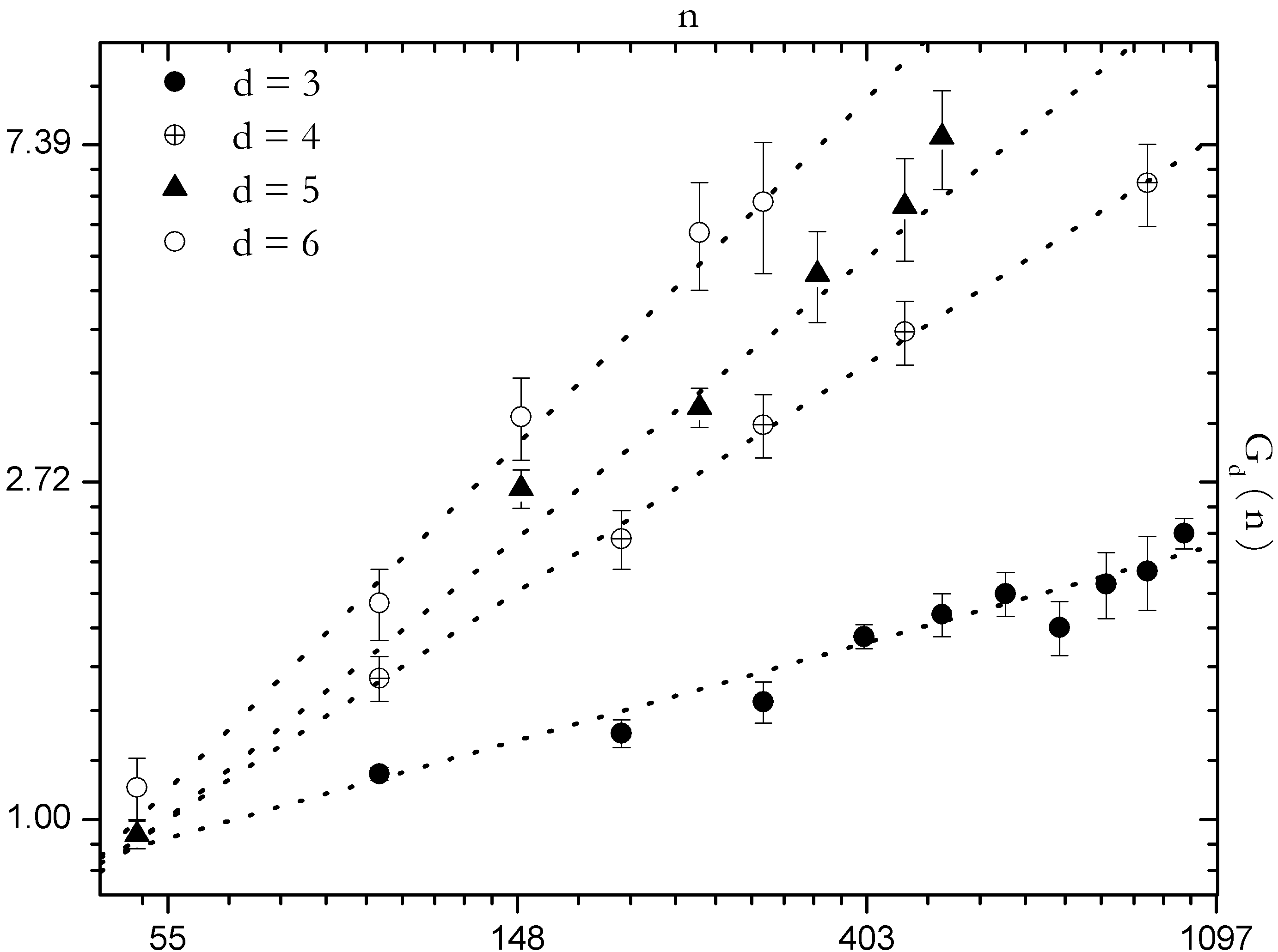
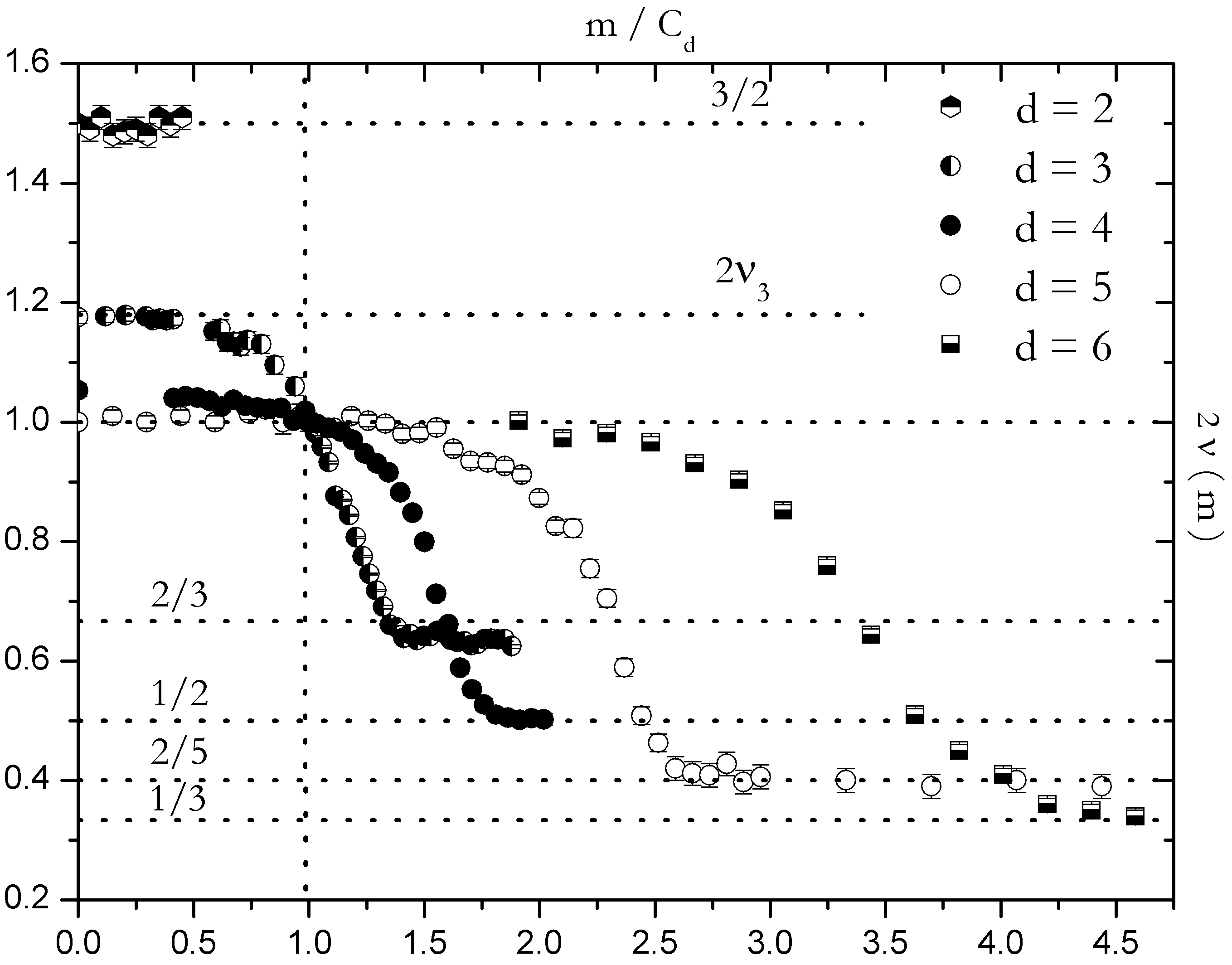
Figure 1: Exponents Ξ½d​(m)subscriptπœˆπ‘‘π‘š\nu_{d}\left(m\right) vs m/Cdπ‘šsubscript𝐢𝑑m/C_{d} from simulations at various lattice dimensions. The graph shows the behavior of Ξ½d​(m)subscriptπœˆπ‘‘π‘š\nu_{d}\left(m\right), obtained from fits of log⁑(⟨Sn2⟩m)subscriptdelimited-⟨⟩superscriptsubscript𝑆𝑛2π‘š\log\left(\langle S_{n}^{2}\rangle_{m}\right) vs log⁑(n)𝑛\log\left(n\right). The range for all fits is n∈[0.8β‹…nM,nM]𝑛⋅0.8subscript𝑛𝑀subscript𝑛𝑀n\in\left[0.8\cdot n_{M},n_{M}\right]. Maximal length for simulated walks was: nM=2β‹…103subscript𝑛𝑀⋅2superscript103n_{M}=2\cdot 10^{3} for d=2𝑑2d=2, nM=103subscript𝑛𝑀superscript103n_{M}=10^{3} for d=3𝑑3d=3, nM=103subscript𝑛𝑀superscript103n_{M}=10^{3} for d=4𝑑4d=4, nM=0.5β‹…103subscript𝑛𝑀⋅0.5superscript103n_{M}=0.5\cdot 10^{3} for d=5𝑑5d=5, and nM=0.3β‹…103subscript𝑛𝑀⋅0.3superscript103n_{M}=0.3\cdot 10^{3} for d=6𝑑6d=6. Moreover, for d=3𝑑3d=3, the log⁑(⟨Sn2⟩m)subscriptdelimited-⟨⟩superscriptsubscript𝑆𝑛2π‘š\log\left(\langle S_{n}^{2}\rangle_{m}\right) has been achieved by using m=C3​M/⟨MnβŸ©π‘šsubscript𝐢3𝑀delimited-⟨⟩subscript𝑀𝑛m=C_{3}M/\langle M_{n}\rangle, with an n𝑛n dependence, to take into account the finite size of the chains (see Fig. (2)). For d>3𝑑3d>3, the finite size effects are much weaker and this correction is not necessary. The picture for d=4𝑑4d=4, m<mcπ‘šsubscriptπ‘šπ‘m<m_{c} shows an exponent slightly larger than 111 (a correction of order π’ͺ​(10βˆ’2)π’ͺsuperscript102\mathcal{O}\left(10^{-2}\right)), consistent with the expected logarithmic correction (for chains of length 103superscript10310^{3} an exponent of 2​ν≃1.070similar-to-or-equals2𝜈1.0702\nu\simeq 1.070 would be predicted). In the nβ†’βˆžβ†’π‘›n\rightarrow\infty limit, Ξ½d​(m)subscriptπœˆπ‘‘π‘š\nu_{d}\left(m\right) is expected to be a step function (see Fig. (3)). The present graph shows the step at mcsubscriptπ‘šπ‘m_{c}: for d=3,4𝑑34d=3,4 we expect mc=Cdsubscriptπ‘šπ‘subscript𝐢𝑑m_{c}=C_{d}, for dβ‰₯5𝑑5d\geq 5 simulations suggest mc>Cdsubscriptπ‘šπ‘subscript𝐢𝑑m_{c}>C_{d}.

Refer to caption
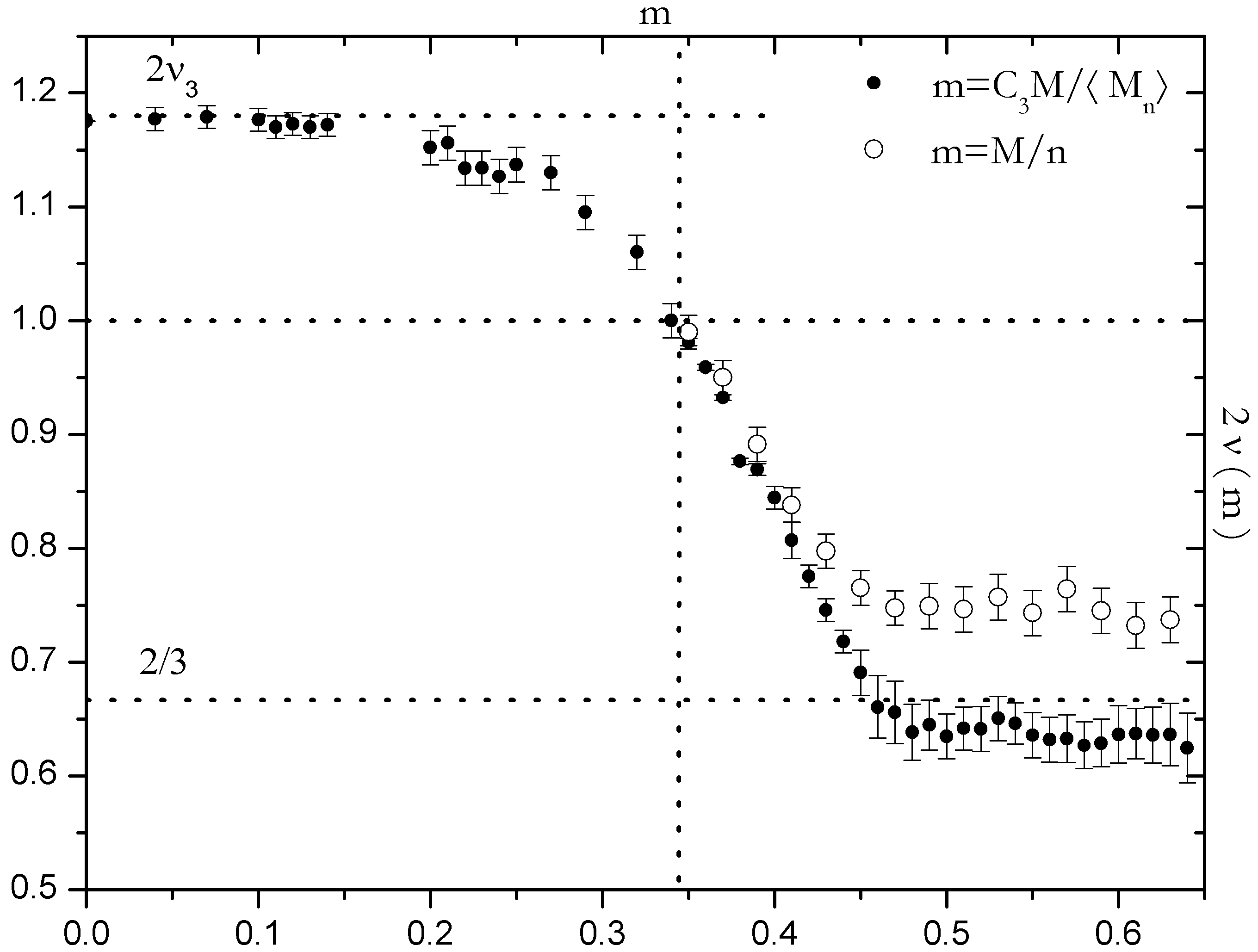
Figure 2: Exponent Ξ½3​(m)subscript𝜈3π‘š\nu_{3}\left(m\right) vs mπ‘šm, a comparison of simulations with and without finite size corrections. The chart, from fits in the form log⁑(⟨Sn2⟩m)subscriptdelimited-⟨⟩superscriptsubscript𝑆𝑛2π‘š\log\left(\langle S_{n}^{2}\rangle_{m}\right) vs log⁑(n)𝑛\log\left(n\right), compares m=M/nπ‘šπ‘€π‘›m=M/n (empty circles) with m=C3​M/⟨MnβŸ©π‘šsubscript𝐢3𝑀delimited-⟨⟩subscript𝑀𝑛m=C_{3}M/\langle M_{n}\rangle (full circles), ⟨Mn⟩delimited-⟨⟩subscript𝑀𝑛\langle M_{n}\rangle is obtained from Eq. (2). Essentially, M𝑀M is rescaled with the average value of the support (range) ⟨Rn⟩=nβˆ’βŸ¨Mn⟩delimited-⟨⟩subscript𝑅𝑛𝑛delimited-⟨⟩subscript𝑀𝑛\langle R_{n}\rangle=n-\langle M_{n}\rangle: this procedure leads to a significant improvement of the accuracy, at least for m>C3π‘šsubscript𝐢3m>C_{3} (vertical dotted line). Given that the two curves in the limit nβ†’βˆžβ†’π‘›n\rightarrow\infty must converge, it is clear that for nM=103subscript𝑛𝑀superscript103n_{M}=10^{3} we are still far from the asymptotic regime. This fact is emphasized in Fig. (3) in which we can see how the drop band for d=3𝑑3d=3 vanishes very slowly compared to d>3𝑑3d>3.
Refer to caption
Figure 3: Slope of Ξ½d​(m)subscriptπœˆπ‘‘π‘š\nu_{d}\left(m\right) in the drop band. The graph shows (in log-log scale) the maximum slope Gd​(n)=βˆ’[βˆ‚mΞ½d​(m)]m​i​nsubscript𝐺𝑑𝑛subscriptdelimited-[]subscriptπ‘šsubscriptπœˆπ‘‘π‘šπ‘šπ‘–π‘›G_{d}\left(n\right)=-\left[\partial_{m}\nu_{d}\left(m\right)\right]_{min} of Ξ½d​(m)subscriptπœˆπ‘‘π‘š\nu_{d}\left(m\right) for different lengths n𝑛n, which is an estimator of the drop band width (proportional to Gdβˆ’1​(n)superscriptsubscript𝐺𝑑1𝑛G_{d}^{-1}\left(n\right)) in which Ξ½d​(m)subscriptπœˆπ‘‘π‘š\nu_{d}(m) falls from Ξ½dsubscriptπœˆπ‘‘\nu_{d} to 1/d1𝑑1/d. Gd​(n)subscript𝐺𝑑𝑛G_{d}\left(n\right) seems to increase with a power law, supporting the idea that Ξ½d​(m)subscriptπœˆπ‘‘π‘š\nu_{d}\left(m\right) is a step function in the limit nβ†’βˆžβ†’π‘›n\rightarrow\infty. Dotted lines are power law Bβ‹…nα⋅𝐡superscript𝑛𝛼B\cdot n^{\alpha} fits to the data: Ξ±=0.29Β±0.01𝛼plus-or-minus0.290.01\alpha=0.29\pm 0.01 for d=3𝑑3d=3 (without the finite size correction C3/⟨Mn⟩subscript𝐢3delimited-⟨⟩subscript𝑀𝑛C_{3}/\langle M_{n}\rangle), Ξ±=0.67Β±0.03𝛼plus-or-minus0.670.03\alpha=0.67\pm 0.03 for d=4𝑑4d=4, Ξ±=0.83Β±0.05𝛼plus-or-minus0.830.05\alpha=0.83\pm 0.05 for d=5𝑑5d=5, and Ξ±=1.02Β±0.07𝛼plus-or-minus1.020.07\alpha=1.02\pm 0.07 for d=6𝑑6d=6. From this data we can notice that the width of the drop band decreases faster in n𝑛n as lattice dimension d𝑑d increases.

III General results

We will briefly discuss the recurrent cases d=1,2𝑑12d=1,2. For d=1𝑑1d=1 we have a rather simple situation: in a linear lattice chain the end-to-end distance is proportional to the range, hence proportional to n𝑛n, βˆ€m<1for-allπ‘š1\forall m<1. A unidimensional SRW is recurrent (C1=1subscript𝐢11C_{1}=1, see Huges ), therefore no drop of Ξ½1​(m)subscript𝜈1π‘š\nu_{1}\left(m\right) is expected for m<1π‘š1m<1. At d=2𝑑2d=2 the picture is conceptually similar. We find Ξ½2​(m)=Ξ½2subscript𝜈2π‘šsubscript𝜈2\nu_{2}\left(m\right)=\nu_{2} (data in Fig. (1)), and since the square lattice SRW is still recurrent (C2=1subscript𝐢21C_{2}=1, from Huges ) from Eq. (4) we expect that this relation holds for any m<1π‘š1m<1 (see later discussion about the case d=3𝑑3d=3).

The most important case is clearly d=3𝑑3d=3: from simulations we find that Ξ½3​(m<mc)=Ξ½3subscript𝜈3π‘šsubscriptπ‘šπ‘subscript𝜈3\nu_{3}\left(m<m_{c}\right)=\nu_{3}, and Ξ½3​(m>mc)=1/3subscript𝜈3π‘šsubscriptπ‘šπ‘13\nu_{3}\left(m>m_{c}\right)=1/3. The last statement needs some attention, we point out that Ξ½3​(m>mc)=1/3subscript𝜈3π‘šsubscriptπ‘šπ‘13\nu_{3}\left(m>m_{c}\right)=1/3 is reached only after a long crossover. Fig. (2) shows ν𝜈\nu vs nβˆ’1​Msuperscript𝑛1𝑀n^{-1}M and C3​M/⟨Mn⟩subscript𝐢3𝑀delimited-⟨⟩subscript𝑀𝑛C_{3}M/\langle M_{n}\rangle: the former does not consider the finite size of the system, while the latter takes into account fluctuations of the walk mean support (range) ⟨Rn⟩delimited-⟨⟩subscript𝑅𝑛\langle R_{n}\rangle at finite n𝑛n (see Franchini-0 ). This enhancement allows a significant improvement of the accuracy for d=3𝑑3d=3 (while is useless in higher dimensions, since, by Eq. (2), the range converges rapidly to its asymptotic behavior).

From Eq. (4) we can locate mcsubscriptπ‘šπ‘m_{c} for d=3𝑑3d=3. If ⟨Sn2⟩msubscriptdelimited-⟨⟩superscriptsubscript𝑆𝑛2π‘š\langle S_{n}^{2}\rangle_{m} has the SAW-like behavior (with Ξ½3>1/2subscript𝜈312\nu_{3}>1/2, see Clisby ) for m<mcπ‘šsubscriptπ‘šπ‘m<m_{c}, and cluster-like for m>mcπ‘šsubscriptπ‘šπ‘m>m_{c}, then the drop of Ξ½3​(m)subscript𝜈3π‘š\nu_{3}\left(m\right) must lie within the range of integration of Eq. (4). It follows that mc=C3subscriptπ‘šπ‘subscript𝐢3m_{c}=C_{3} for nβ†’βˆžβ†’π‘›n\rightarrow\infty. As for the exponent at the critical point, Eq. (4) tells us that Ξ½d​(mβ†’Cd)=1/2subscriptπœˆπ‘‘β†’π‘šsubscript𝐢𝑑12\nu_{d}\left(m\rightarrow C_{d}\right)=1/2, from which it follows that Ξ½3​(mc)=1/2subscript𝜈3subscriptπ‘šπ‘12\nu_{3}\left(m_{c}\right)=1/2: this observation is supported by Fig. (1) and (2), where we see that 2​ν3​(m)2subscript𝜈3π‘š2\nu_{3}\left(m\right) passes through 111 at the expected critical point mc=C3subscriptπ‘šπ‘subscript𝐢3m_{c}=C_{3}.

This latter fact is of some importance, since the transition for d=3𝑑3d=3 would show the same behavior as that described by the Hamiltonian in Eq. (1). If the two models belong to the same universality class this would be very interesting, since in our model the transition arises from the necessity of maximizing the configurational entropy, without the need for any further interactions. Indeed, at the critical point mcsubscriptπ‘šπ‘m_{c} there is a radical change in the optimal strategy to achieve the global constraint mπ‘šm (which is actually a long-range correlation): for m<mcπ‘šsubscriptπ‘šπ‘m<m_{c}, the best way to change the ratio mπ‘šm is to compress (or expand) the chain locally, keeping the SAW-like fractal structure. In this situation the monomers intersect (on average) only within a certain distance along the chain. For m>mcπ‘šsubscriptπ‘šπ‘m>m_{c} instead, it becomes entropically convenient to assume a compact configuration, also allowing intersections between monomers very far apart in terms of position along the chain.

We also studied higher dimensions, the results are consistent with a CG transition of the same kind. For d=4𝑑4d=4 we have Ξ½4​(m>mc)=1/4subscript𝜈4π‘šsubscriptπ‘šπ‘14\nu_{4}\left(m>m_{c}\right)=1/4 and Ξ½4​(m<mc)=1/2subscript𝜈4π‘šsubscriptπ‘šπ‘12\nu_{4}\left(m<m_{c}\right)=1/2, but the random-coil behavior shows logarithmic corrections. Simulations fit the conjecture that ⟨Sn2⟩m∝nlog(n)1/4\langle S_{n}^{2}\rangle_{m}\propto n\log\left(n\right)^{1/4}, as in the SAW case Madras-Slade . If this is true, from Eq. (4), we should again find mc=C4subscriptπ‘šπ‘subscript𝐢4m_{c}=C_{4}.

As expected, for dβ‰₯5𝑑5d\geq 5, m<mcπ‘šsubscriptπ‘šπ‘m<m_{c}, we find the mean field behavior Ξ½d​(m)=1/2subscriptπœˆπ‘‘π‘š12\nu_{d}\left(m\right)=1/2 (as for the SRW), and Ξ½d​(m)=1/dsubscriptπœˆπ‘‘π‘š1𝑑\nu_{d}\left(m\right)=1/d for m>mcπ‘šsubscriptπ‘šπ‘m>m_{c}. Since for dβ‰₯5𝑑5d\geq 5 Ξ½d​(m<mc)subscriptπœˆπ‘‘π‘šsubscriptπ‘šπ‘\nu_{d}\left(m<m_{c}\right) is the same as for the SRW, we neither use Eq. (4) to locate mcsubscriptπ‘šπ‘m_{c} nor find Ξ½d​(mc)subscriptπœˆπ‘‘subscriptπ‘šπ‘\nu_{d}\left(m_{c}\right), but our simulations (extremes of the drop zone of Ξ½d​(m)subscriptπœˆπ‘‘π‘š\nu_{d}\left(m\right), d=5,6𝑑56d=5,6 in Fig. (1)) strongly suggest that mc>Cdsubscriptπ‘šπ‘subscript𝐢𝑑m_{c}>C_{d}. All results and conjectures about the behavior of ⟨Sn2⟩msubscriptdelimited-⟨⟩superscriptsubscript𝑆𝑛2π‘š\langle S_{n}^{2}\rangle_{m} have been summarised in Table I.

d𝑑d ν​(m<mc)πœˆπ‘šsubscriptπ‘šπ‘\nu\left(m<m_{c}\right) ν​(m=mc)πœˆπ‘šsubscriptπ‘šπ‘\nu\left(m=m_{c}\right) ν​(m>mc)πœˆπ‘šsubscriptπ‘šπ‘\nu\left(m>m_{c}\right) mc/Cdsubscriptπ‘šπ‘subscript𝐢𝑑m_{c}/C_{d}
333 ν3subscript𝜈3\nu_{3} 1/2121/2 1/3131/3 111
444         1/2l.c.1subscript2formulae-sequence𝑙𝑐\,\,\,\,\,\,\,\,1/2\,_{l.c.} 1/2121/2 1/4141/4 111
555 1/2121/2 βˆ’- 1/5151/5 1.5∽2.7∽1.52.71.5\backsim 2.7
666 1/2121/2 βˆ’- 1/6161/6 2.1∽4.4∽2.14.42.1\backsim 4.4
Tabella 1: Summary of predictions for Ξ½d​(m)subscriptπœˆπ‘‘π‘š\nu_{d}\left(m\right): for d=5,6𝑑56d=5,6 we where unable to look at the critical behavior, while the critical point mcsubscriptπ‘šπ‘m_{c} is evaluated by the drop zone of Ξ½d​(m)subscriptπœˆπ‘‘π‘š\nu_{d}\left(m\right). The l.c. indicates SAW logarithmic correction in d=4𝑑4d=4.

We would like to point out that all results for dβ‰₯3𝑑3d\geq 3, mβ‰₯mcπ‘šsubscriptπ‘šπ‘m\geq m_{c}, are consistent with a remarkable exact work by M. van den Berg, E. Bolthausen and F. den Hollander (den Hollander ) on the moderate deviations for the volume of a Wiener Sausage (WS), which is a neighborhood of the trace of a standard Brownian motion up to a time t𝑑t, given by taking all points within a fixed distance aπ‘Ža of Brownian motion (essentially a continuous version of our model, see Franchini-1 ). Let η​(t)πœ‚π‘‘\eta\left(t\right), tβ‰₯0𝑑0t\geq 0 be the standard Brownian motion in ℝdsuperscriptℝ𝑑\mathbb{R}^{d} starting at the origin. The WS Wa​(t)superscriptπ‘Šπ‘Žπ‘‘W^{a}\left(t\right) with radius aπ‘Ža is the process defined by

Wa​(t)=⋃0≀s≀tBa​(η​(s)),superscriptπ‘Šπ‘Žπ‘‘subscript0𝑠𝑑subscriptπ΅π‘Žπœ‚π‘ W^{a}\left(t\right)=\bigcup_{0\leq s\leq t}B_{a}(\eta\left(s\right)), (5)

where Ba​(x)subscriptπ΅π‘Žπ‘₯B_{a}\left(x\right) is the open ball with radius aπ‘Ža around xβˆˆβ„dπ‘₯superscriptℝ𝑑x\in\mathbb{R}^{d}. This paper considers the probability of having a Wiener Sausage Wa​(t)superscriptπ‘Šπ‘Žπ‘‘W^{a}\left(t\right) of volume |Wa​(t)|≀b​tsuperscriptπ‘Šπ‘Žπ‘‘π‘π‘‘\left|W^{a}\left(t\right)\right|\leq bt, b∈[0,ΞΊa]𝑏0subscriptπœ…π‘Žb\in\left[0,\kappa_{a}\right] (ΞΊa​tsubscriptπœ…π‘Žπ‘‘\kappa_{a}t is the long time behavior of ⟨|Wa​(t)|⟩delimited-⟨⟩superscriptπ‘Šπ‘Žπ‘‘\langle\left|W^{a}\left(t\right)\right|\rangle), showing that there exists a critical value bcsubscript𝑏𝑐b_{c} below which the sausage is supposed to collapse in a swiss-cheese like compact configuration (a non-percolating cluster with random holes of size π’ͺ​(1)π’ͺ1\mathcal{O}\left(1\right)). They rigorously showed that bc∈(0,ΞΊd)subscript𝑏𝑐0subscriptπœ…π‘‘b_{c}\in\left(0,\kappa_{d}\right) for dβ‰₯5𝑑5d\geq 5 only, while for d=3,4𝑑34d=3,4 the transition is at bc=ΞΊasubscript𝑏𝑐subscriptπœ…π‘Žb_{c}=\kappa_{a} exactly.

IV Order parameter

Typically the order parameter considered for a CG transition is nβˆ’1β€‹βŸ¨Sn2⟩βsuperscript𝑛1subscriptdelimited-⟨⟩superscriptsubscript𝑆𝑛2𝛽n^{-1}\langle S_{n}^{2}\rangle_{\beta} (with βŸ¨β‹…βŸ©Ξ²subscriptdelimited-βŸ¨βŸ©β‹…π›½\langle\cdot\rangle_{\beta} being the thermodynamic average); we propose here a slightly different parameter:

Ο±d​(m)=limnβ†’βˆžβŸ¨Sn2⟩m/⟨Sn2⟩0.subscriptitalic-Ο±π‘‘π‘šsubscript→𝑛subscriptdelimited-⟨⟩superscriptsubscript𝑆𝑛2π‘šsubscriptdelimited-⟨⟩superscriptsubscript𝑆𝑛20\varrho_{d}\left(m\right)=\lim_{n\rightarrow\infty}\sqrt{\langle S_{n}^{2}\rangle_{m}/\langle S_{n}^{2}\rangle_{0}}. (6)

This function vanishes beyond the critical point, similarly to the magnetization for spin systems. If the analogy with the CG transition from Eq. (1) holds, we should expect a second order transition, at least for d=3𝑑3d=3.

Refer to caption
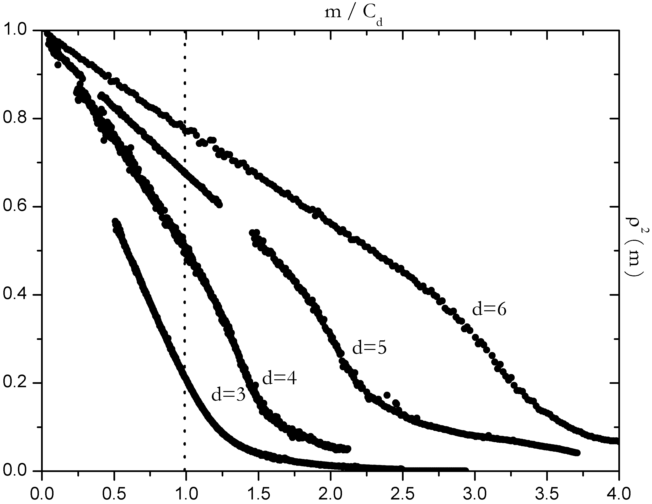
Figure 4: Order parameter Ο±d​(m)subscriptitalic-Ο±π‘‘π‘š\varrho_{d}\left(m\right) vs m/Cdπ‘šsubscript𝐢𝑑m/C_{d} from simulations at various lattice dimensions. The graph shows ⟨Sn2⟩m/⟨Sn2⟩0subscriptdelimited-⟨⟩superscriptsubscript𝑆𝑛2π‘šsubscriptdelimited-⟨⟩superscriptsubscript𝑆𝑛20\langle S_{n}^{2}\rangle_{m}/\langle S_{n}^{2}\rangle_{0}: n=103𝑛superscript103n=10^{3} for d=3𝑑3d=3, n=2β‹…103𝑛⋅2superscript103n=2\cdot 10^{3} for d=4𝑑4d=4, n=103𝑛superscript103n=10^{3} for d=5𝑑5d=5 and n=0.5β‹…103𝑛⋅0.5superscript103n=0.5\cdot 10^{3} for d=6𝑑6d=6. The vertical dotted line is the expected transition point for d=3,4𝑑34d=3,4 as nβ†’βˆžβ†’π‘›n\rightarrow\infty. The asymptotic behavior near mcsubscriptπ‘šπ‘m_{c} is only hinted, since our PERM implementation, which requires us to store the microcanonical density of states at many n𝑛n, has not allowed us to simulate longer chains. Better pictures could surely be achieved, by more focused techniques, for every dimensions except d=4𝑑4d=4. For d=4𝑑4d=4 and m<C4π‘šsubscript𝐢4m<C_{4} we expect nβˆ’1β€‹βŸ¨Sn2⟩msuperscript𝑛1subscriptdelimited-⟨⟩superscriptsubscript𝑆𝑛2π‘šn^{-1}\langle S_{n}^{2}\rangle_{m} to be only π’ͺ(log(n)1/4)\mathcal{O}(\log\left(n\right)^{1/4}), implying the asymptotic behavior would be difficult to demonstrate clearly even by simulation for very large chains.

Our simulations (Fig. (4)) do not allow us to clarify if the transition is continuous at mcsubscriptπ‘šπ‘m_{c}. However, for d=3𝑑3d=3 we can get some insights by a mean field analysis of the Stanley Model (SM, see Franchini-2 ), a model of correlated random walks defined by the following partition function:

𝒡n​(Ξ²)βˆβˆ‘M=0nPn​(M)​eβˆ’Ξ²β€‹M.proportional-tosubscript𝒡𝑛𝛽superscriptsubscript𝑀0𝑛subscript𝑃𝑛𝑀superscript𝑒𝛽𝑀\mathcal{Z}_{n}\left(\beta\right)\propto\sum_{M=0}^{n}P_{n}\left(M\right)e^{-\beta M}. (7)

Given that variable ΞΎπœ‰\xi in Eq. (3) is normally-distributed, it’s easy to show that for small β𝛽\beta

limnβ†’βˆžnβˆ’1β€‹βŸ¨MnβŸ©Ξ²β‰ƒC3βˆ’Ξ΄β€‹m​(Ξ²),similar-to-or-equalssubscript→𝑛superscript𝑛1subscriptdelimited-⟨⟩subscript𝑀𝑛𝛽subscript𝐢3π›Ώπ‘šπ›½\lim_{n\rightarrow\infty}n^{-1}\langle M_{n}\rangle_{\beta}\simeq C_{3}-\delta m\left(\beta\right), (8)

where ⟨Mn⟩βsubscriptdelimited-⟨⟩subscript𝑀𝑛𝛽\langle M_{n}\rangle_{\beta} is the mean number of intersections in the SM at temperature β𝛽\beta, and δ​m​(Ξ²)π›Ώπ‘šπ›½\delta m\left(\beta\right) vanishes for Ξ²β†’0→𝛽0\beta\rightarrow 0. From Eq. (3) we have a Gaussian shape Pn​(M)subscript𝑃𝑛𝑀P_{n}\left(M\right) near M=C3​n𝑀subscript𝐢3𝑛M=C_{3}n, with βŸ¨Ξ”β€‹Mn2⟩∝n​log⁑(n)proportional-todelimited-βŸ¨βŸ©Ξ”superscriptsubscript𝑀𝑛2𝑛𝑛\langle\Delta M_{n}^{2}\rangle\propto n\log\left(n\right). By replacing Mβ†’m​nβ†’π‘€π‘šπ‘›M\rightarrow mn in Eq. (7) we find

𝒡n​(Ξ²)∝∫01𝑑m​eβˆ’n2​[2​β​m+nβ€‹βŸ¨Ξ”β€‹Mn2βŸ©βˆ’1​δ​m2]proportional-tosubscript𝒡𝑛𝛽superscriptsubscript01differential-dπ‘šsuperscript𝑒𝑛2delimited-[]2π›½π‘šπ‘›superscriptdelimited-βŸ¨βŸ©Ξ”superscriptsubscript𝑀𝑛21𝛿superscriptπ‘š2\mathcal{Z}_{n}\left(\beta\right)\propto\int_{0}^{1}dm\,e^{-\frac{n}{2}\left[2\beta m+n\langle\Delta M_{n}^{2}\rangle^{-1}\delta m^{2}\right]} (9)

for small β𝛽\beta, with δ​m=(C3βˆ’m)≃0π›Ώπ‘šsubscript𝐢3π‘šsimilar-to-or-equals0\delta m=\left(C_{3}-m\right)\simeq 0. Whereas there is a positive constant a0subscriptπ‘Ž0a_{0} such that βŸ¨Ξ”β€‹Mn2⟩>a0​ndelimited-βŸ¨βŸ©Ξ”superscriptsubscript𝑀𝑛2subscriptπ‘Ž0𝑛\langle\Delta M_{n}^{2}\rangle>a_{0}n for large n𝑛n, performing a saddle point integration on Eq. (9) with nβ†’βˆžβ†’π‘›n\rightarrow\infty we obtain δ​m​(Ξ²)>c0β€‹Ξ²π›Ώπ‘šπ›½subscript𝑐0𝛽\delta m\left(\beta\right)>c_{0}\beta (for small β𝛽\beta and c0>0subscript𝑐00c_{0}>0).

From simple mean field arguments (see Franchini-3 ) it is reasonable to assume that the SM can be approximately described by the Flory theory. Consider the following Flory energy

ℱβ​(r)βˆΌΞ²β€‹n2​rβˆ’d+r22​nβˆ’(dβˆ’1)​log⁑(r)+Λ​(n),similar-tosubscriptβ„±π›½π‘Ÿπ›½superscript𝑛2superscriptπ‘Ÿπ‘‘superscriptπ‘Ÿ22𝑛𝑑1π‘ŸΞ›π‘›\mathcal{F}_{\beta}\left(r\right)\sim\beta n^{2}r^{-d}+\frac{r^{2}}{2n}-\left(d-1\right)\log\left(r\right)+\Lambda\left(n\right), (10)

where r=|Sn|π‘Ÿsubscript𝑆𝑛r=\left|S_{n}\right| is the end-to-end distance, and Λ​(n)Λ𝑛\Lambda\left(n\right) is a function independent of rπ‘Ÿr Madras-Slade . We minimize the functional under the assumption rβˆΌΞ²ΞΈβ€‹nΞ½βˆΌπ‘Ÿsuperscriptπ›½πœƒsuperscriptπ‘›πœˆr\thicksim\beta^{\theta}n^{\nu}, thus

d​β1βˆ’ΞΈβ€‹(1+d)​n2βˆ’Ξ½β€‹(1+d)+(dβˆ’1)β€‹Ξ²βˆ’ΞΈβ€‹nβˆ’Ξ½=βθ​nΞ½βˆ’1.𝑑superscript𝛽1πœƒ1𝑑superscript𝑛2𝜈1𝑑𝑑1superscriptπ›½πœƒsuperscriptπ‘›πœˆsuperscriptπ›½πœƒsuperscriptπ‘›πœˆ1d\beta^{1-\theta\left(1+d\right)}n^{2-\nu\left(1+d\right)}+\left(d-1\right)\beta^{-\theta}n^{-\nu}=\beta^{\theta}n^{\nu-1}. (11)

When ν​d<2πœˆπ‘‘2\nu d<2 we find Ξ½=3/(d+2)𝜈3𝑑2\nu=3/\left(d+2\right) and ΞΈ=1/(d+2)πœƒ1𝑑2\theta=1/\left(d+2\right), otherwise Ξ½=1/2𝜈12\nu=1/2 and ΞΈ=0πœƒ0\theta=0. When d=3𝑑3d=3 this theory predicts ΞΈ=1/5πœƒ15\theta=1/5. A different estimation method uses path integrals, results are in agreement Kleinhert .

Flory theory for SM where d=3𝑑3d=3 predicts ⟨Sn2⟩β∝β2/5​n6/5proportional-tosubscriptdelimited-⟨⟩superscriptsubscript𝑆𝑛2𝛽superscript𝛽25superscript𝑛65\langle S_{n}^{2}\rangle_{\beta}\propto\beta^{2/5}n^{6/5} for small β𝛽\beta: inverting δ​m​(Ξ²)π›Ώπ‘šπ›½\delta m\left(\beta\right), and substituting in the expression for ⟨Sn2⟩βsubscriptdelimited-⟨⟩superscriptsubscript𝑆𝑛2𝛽\langle S_{n}^{2}\rangle_{\beta}, we find Ο±3​(m)<b0​δ​m1/5subscriptitalic-Ο±3π‘šsubscript𝑏0𝛿superscriptπ‘š15\varrho_{3}\left(m\right)<b_{0}\delta m^{1/5}, with δ​m=(C3βˆ’m)≃0π›Ώπ‘šsubscript𝐢3π‘šsimilar-to-or-equals0\delta m=\left(C_{3}-m\right)\simeq 0, b0>0subscript𝑏00b_{0}>0.

In the case d=4𝑑4d=4 Flory theory cannot be used, since the logarithmic correction to the mean field behavior are not captured. Note that the dβ‰₯5𝑑5d\geq 5 theory predicts ΞΈ=0πœƒ0\theta=0, in agreement with the prediction mc>Cdsubscriptπ‘šπ‘subscript𝐢𝑑m_{c}>C_{d} for dβ‰₯5𝑑5d\geq 5.

The exponents found are certainly incorrect, since Ξ½3β‰ 3/5subscript𝜈335\nu_{3}\neq 3/5, but a power law behavior Ο±3​(m)βˆΞ΄β€‹mΞΈproportional-tosubscriptitalic-Ο±3π‘šπ›Ώsuperscriptπ‘šπœƒ\varrho_{3}\left(m\right)\propto\delta m^{\theta} (with a likely logarithmic correction) is reasonable, suggesting that in d=3𝑑3d=3 the transition is of the second order, with mc=C3subscriptπ‘šπ‘subscript𝐢3m_{c}=C_{3}.

V Conclusion and outlook

In this paper we introduced a new athermal model of interacting random walks, which shows a CG transition for a critical ratio between the range and the number of monomers. The transition seems to show the same characteristics as that seen in canonical models. However, the relationship between our microcanonical model and those canonical for the CG transition is non-trivial (for a general discussion on the differences between microcanonical and canonical ensembles see Touchette ).

The Hamiltonian in Eq. (1), as well as the interaction described in reference Krawckzyk , operate a selection on the ensemble ΩΩ\Omega whose mechanisms are not easily connected to the ensemble Ξ©msubscriptΞ©π‘š\Omega_{m}. Although this is a key issue, we do not discuss it here: a work dedicated to this subject is currently under preparation, where we will present a detailed study of the Pn​(m)subscriptπ‘ƒπ‘›π‘šP_{n}\left(m\right) distribution and its relation to some thermodynamic models.

Apart from more focused implementation of the simulations here presented, other issues of interest could affect the connectivity properties of collapsed clusters (an example is found in den Hollander , collapsed WS clusters should be non-percolating, with π’ͺ​(n)π’ͺ𝑛\mathcal{O}\left(n\right) holes sized π’ͺ​(1)π’ͺ1\mathcal{O}\left(1\right) distributed inside the range: is reasonable to expect the same behavior for our model when m>mcπ‘šsubscriptπ‘šπ‘m>m_{c}).

In general, this model certainly deserves attention since, in our opinion, it could lead to substantial improvements in understanding the geometry of CG transitions, as well as the crossover between the SAW and the SRW.

VI Acknowledgments

We thank Frank den Hollander (University of Leiden) for suggesting the finite-size correction to improve simulations in d=3𝑑3d=3, and Jack F. Douglas (NIST) for fundamental clarifications about the current theory of the CG transition. We also thank Riccardo Balzan (EPFL) and Giorgio Parisi (Sapienza UniversitΓ  di Roma) for interesting discussions.

References

  • (1) J. des Cloizeaux and G. Jannink, Polymers in solutions: Their Modelling and Structure, Clarendon Press, Oxford (1990)
  • (2) P. G. de Gennes, Scaling Concepts in Polymer Physics, Cornell University Press (1979)
  • (3) A. Y. Grosberg and D. V. Kuznetsov, Macromolecules 25, 1970 (1992)
  • (4) B. D. Hughes, Random Walks and Random Enviroments, Vol.1 Clarendon Press, Oxford (1995)
  • (5) J. Krawczyk, T. Prellberg, A. L. Owczarek and A. Rechnitzer, Phys. Rev. Lett. 96, 240603 (2006)
  • (6) Our simulations have been performed by using the Pruned-Enriched Rosenbluth Method (PERM), a stochastic growth algorithm that combines the Rosenbluth-Rosenbluth method (which simulate a biased sample, and correct the bias by means of a weight associated to each configuration) with recursive enrichment, starting off building instances according to a biased distribution, but correcting for this by cloning desired (enriching) and killing undesired configurations (pruning) in order to contain the weights fluctuations of the simulated samples: see Grassberger ; Prellberg ; Hsu-Grassberger for reviews and Grassberger for a pseudocode.
  • (7) P. Grassberger, Phys. Rev. E 56, 3682 (1997)
  • (8) T. Prellberg and J. Krawczyk, Phys. Rev. Lett. 92, 120602 (2004)
  • (9) H.-P. Hsu and P. Grassberger, J. Stat. Phys. 144, 597 (2011)
  • (10) N. Madras and G. Slade, The Self-Avoiding Walk, Birkhauser, Boston (1996)
  • (11) N. Clisby, Phys. Rev. Lett. 104, 055702 (2010)
  • (12) A. L. Owczarek and T. Prellberg, J. Phys. A: Math. Gen. 34, 5773 (2001)
  • (13) J. F. Douglas and T. Ishinabe, Phys. Rev. E 51, 1791 (1995)
  • (14) N. C. Jain and W. E. Pruitt, J. Analyse Math. 24, 369 (1971)
  • (15) The optimal correction would actually be m=1βˆ’CΒ―3​R/⟨RnβŸ©π‘š1subscript¯𝐢3𝑅delimited-⟨⟩subscript𝑅𝑛m=1-\bar{C}_{3}R/\langle R_{n}\rangle instead of m=C3​M/⟨MnβŸ©π‘šsubscript𝐢3𝑀delimited-⟨⟩subscript𝑀𝑛m=C_{3}M/\langle M_{n}\rangle but, since they differ only by π’ͺ​(nβˆ’1)π’ͺsuperscript𝑛1\mathcal{O}(n^{-1}) compared to a leading order of π’ͺ​(nβˆ’1/2)π’ͺsuperscript𝑛12\mathcal{O}(n^{-1/2}), we preferred to use the second option to simplify the data analysis.
  • (16) M. van den Berg, E. Bolthausen and F. den Hollander, Ann. Math. 153, 355 (2001)
  • (17) The volume of a Wiener Sausage is the continuous analogue of the range in SRW: the condition |Wa​(t)|≀b​tsuperscriptπ‘Šπ‘Žπ‘‘π‘π‘‘\left|W^{a}\left(t\right)\right|\leq bt, b∈[0,ΞΊa]𝑏0subscriptπœ…π‘Žb\in\left[0,\kappa_{a}\right] is equivalent to R​[Ο‰]≀(1βˆ’m)​n𝑅delimited-[]πœ”1π‘šπ‘›R\left[\omega\right]\leq\left(1-m\right)n, m∈[0,Cd]π‘š0subscript𝐢𝑑m\in\left[0,C_{d}\right] (then M​[Ο‰]β‰₯m​n𝑀delimited-[]πœ”π‘šπ‘›M\left[\omega\right]\geq mn) in our model. For a brief review on the Wiener Sausage see den Hollander .
  • (18) The Stanley Model (SM, see Stanley for the original formulation, or Huges for a review) is a model of correlated random walks which describes polymer chains with either repulsion or attractions. The attractive case is mathematically equivalent to the Rosenstock Trapping Model (random walk on lattice with randomly distributed irreversible traps: a walker encountering a trap is killed there, see Huges ) and has been exactly solved by M. D. Donsker and S. R. S. Varadhan Donsker-Varadhan .
  • (19) H. E. Stanley, K. Kang, S. Redner and R. L. Blumberg, Phys. Rev. Lett. 51, 1223 (1983); Erratum: ibid. 54, 1209 (1985)
  • (20) M. D. Donsker and S. R. S. Varadhan, Comm. Pure. Appl. Math. 28, 525 (1975); Erratum: ibid. 28, 667 (1975)
  • (21) We show that for small β𝛽\beta the SM is described by the same mean field theory of the Domb-Joyce Model (see Huges for a review of this important model), therefore by the Flory Theory. We start from the Domb-Joyce Hamiltonian β„‹D​J=Ο΅β€‹βˆ‘xψx2=Ο΅β€‹βˆ‘xRxβ€‹Οˆx2subscriptℋ𝐷𝐽italic-Ο΅subscriptπ‘₯superscriptsubscriptπœ“π‘₯2italic-Ο΅subscriptπ‘₯subscript𝑅π‘₯superscriptsubscriptπœ“π‘₯2\mathcal{H}_{DJ}=\epsilon\sum_{x}\psi_{x}^{2}=\epsilon\sum_{x}R_{x}\psi_{x}^{2}, with Rx=limΞ³β†’0ψxΞ³subscript𝑅π‘₯subscript→𝛾0superscriptsubscriptπœ“π‘₯𝛾R_{x}=\lim_{\gamma\rightarrow 0}\psi_{x}^{\gamma} and ψxsubscriptπœ“π‘₯\psi_{x} the same of Eq. (1): approximating ψxβ†’ΟˆΒ―=n​Rβˆ’1β†’subscriptπœ“π‘₯Β―πœ“π‘›superscript𝑅1\psi_{x}\rightarrow\bar{\psi}=nR^{-1} we have β„‹D​JβˆΌΟ΅β€‹Rβ€‹ΟˆΒ―2similar-tosubscriptℋ𝐷𝐽italic-ϡ𝑅superscriptΒ―πœ“2\mathcal{H}_{DJ}\sim\epsilon R\bar{\psi}^{2}, where ΟˆΒ―Β―πœ“\bar{\psi} is the average occupation of a visited site, and R=βˆ‘xRx𝑅subscriptπ‘₯subscript𝑅π‘₯R=\sum_{x}R_{x} is the range. It follows that β„‹D​JβˆΌΟ΅β€‹n​(1βˆ’m)βˆ’1similar-tosubscriptℋ𝐷𝐽italic-ϡ𝑛superscript1π‘š1\mathcal{H}_{DJ}\sim\epsilon n\left(1-m\right)^{-1}, while the Hamiltonian of the SM is β„‹S​M=βˆ’Ο΅β€‹n​msubscriptℋ𝑆𝑀italic-Ο΅π‘›π‘š\mathcal{H}_{SM}=-\epsilon nm. For small β𝛽\beta we have to consider m=Cdβˆ’Ξ΄β€‹mπ‘šsubscriptπΆπ‘‘π›Ώπ‘šm=C_{d}-\delta m, and substituting this expression in β„‹D​Jsubscriptℋ𝐷𝐽\mathcal{H}_{DJ}, β„‹S​Msubscriptℋ𝑆𝑀\mathcal{H}_{SM} we find δ​ℋD​JβˆΞ΄β€‹β„‹S​Mproportional-to𝛿subscriptℋ𝐷𝐽𝛿subscriptℋ𝑆𝑀\delta\mathcal{H}_{DJ}\propto\delta\mathcal{H}_{SM}, from which it follows that the two models are equivalent in mean field description, with different couplings Ο΅italic-Ο΅\epsilon.
  • (22) H. Kleinert, Path Integrals in Quantum Mechanics, Statistics, and Polymer Physics, World Scientific (1990)
  • (23) H. Touchette, Equivalence and Nonequivalence of the Microcanonical and Canonical Ensembles: A Large Deviations Study, Ph.D. Thesis, McGill University, MontrΓ©al (2003)