Making Gradient Descent Optimal
for Strongly Convex Stochastic Optimization
Abstract
Stochastic gradient descent (SGD) is a simple and popular method to solve stochastic optimization problems which arise in machine learning. For strongly convex problems, its convergence rate was known to be , by running SGD for iterations and returning the average point. However, recent results showed that using a different algorithm, one can get an optimal rate. This might lead one to believe that standard SGD is suboptimal, and maybe should even be replaced as a method of choice. In this paper, we investigate the optimality of SGD in a stochastic setting. We show that for smooth problems, the algorithm attains the optimal rate. However, for non-smooth problems, the convergence rate with averaging might really be , and this is not just an artifact of the analysis. On the flip side, we show that a simple modification of the averaging step suffices to recover the rate, and no other change of the algorithm is necessary. We also present experimental results which support our findings, and point out open problems.
1 Introduction
Stochastic gradient descent (SGD) is one of the simplest and most popular first-order methods to solve convex learning problems. Given a convex loss function and a training set of examples, SGD can be used to obtain a sequence of predictors, whose average has a generalization error which converges (with ) to the optimal one in the class of predictors we consider. The common framework to analyze such first-order algorithms is via stochastic optimization, where our goal is to optimize an unknown convex function , given only unbiased estimates of ’s subgradients (see Sec. 2 for a more precise definition).
An important special case is when is strongly convex (intuitively, can be lower bounded by a quadratic function). Such functions arise, for instance, in Support Vector Machines and other regularized learning algorithms. For such problems, there is a well-known convergence guarantee for SGD with averaging. This rate is obtained using the analysis of the algorithm in the harder setting of online learning Hazan et al. (2007), combined with an online-to-batch conversion (see Hazan & Kale (2011) for more details).
Surprisingly, a recent paper by Hazan and Kale Hazan & Kale (2011) showed that in fact, an is not the best that one can achieve for strongly convex stochastic problems. In particular, an optimal rate can be obtained using a different algorithm, which is somewhat similar to SGD but is more complex (although with comparable computational complexity)111Roughly speaking, the algorithm divides the iterations into exponentially increasing epochs, and runs stochastic gradient descent with averaging on each one. The resulting point of each epoch is used as the starting point of the next epoch. The algorithm returns the resulting point of the last epoch.. A very similar algorithm was also presented recently by Juditsky and Nesterov Juditsky & Nesterov (2010).
These results left an important gap: Namely, whether the true convergence rate of SGD, possibly with some sort of averaging, might also be , and the known result is just an artifact of the analysis. Indeed, the whole motivation of Hazan & Kale (2011) was that the standard online analysis is too loose to analyze the stochastic setting properly. Perhaps a similar looseness applies to the analysis of SGD as well? This question has immediate practical relevance: if the new algorithms enjoy a better rate than SGD, it might indicate they will work better in practice, and that practitioners should abandon SGD in favor of them.
In this paper, we study the convergence rate of SGD for stochastic strongly convex problems, with the following contributions:
-
•
First, we extend known results to show that if is not only strongly convex, but also smooth (with respect to the optimum), then SGD with and without averaging achieves the optimal convergence rate.
-
•
We then show that for non-smooth , there are cases where the convergence rate of SGD with averaging is . In other words, the bound for general strongly convex problems is real, and not just an artifact of the currently-known analysis.
-
•
However, we show that one can recover the optimal convergence rate by a simple modification of the averaging step: Instead of averaging of points, we only average the last points, where is arbitrary. Thus, to obtain an optimal rate, one does not need to use an algorithm significantly different than SGD, such as those discussed earlier.
-
•
We perform an empirical study on both artificial and real-world data, which supports our findings.
Following the paradigm of Hazan & Kale (2011), we analyze the algorithm directly in the stochastic setting, and avoid an online analysis with an online-to-batch conversion. Our rate upper bounds are shown to hold in expectation, but we also sketch how we can obtain high-probability bounds (up to a factor). While the focus here is on getting the optimal rate in terms of , we note that our upper bounds are also optimal in terms of other standard problem parameters, such as the strong convexity parameter and the variance of the stochastic gradients.
In terms of related work, we note that the performance of SGD in a stochastic setting has been extensively researched in stochastic approximation theory (see for instance Kushner & Yin (2003)). However, these results are usually obtained under smoothness assumptions, and are often asymptotic, so we do not get an explicit bound in terms of which applies to our setting. We also note that a finite-sample analysis of SGD in the stochastic setting was recently presented in Bach & Moulines (2011). However, the focus there was different than ours, and also obtained bounds which hold only in expectation rather than in high probability. More importantly, the analysis was carried out under stronger smoothness assumptions than our analysis, and to the best of our understanding, does not apply to general, possibly non-smooth, strongly convex stochastic optimization problems. For example, smoothness assumptions may not cover the application of SGD to support vector machines (as in Shalev-Shwartz et al. (2011)), since it uses a non-smooth loss function, and thus the underlying function we are trying to stochastically optimize may not be smooth.
2 Preliminaries
We use bold-face letters to denote vectors. Given some vector , we use to denote its -th coordinate. Similarly, given some indexed vector , we let denote its -th coordinate. We let denote the indicator function for some event .
We consider the standard setting of convex stochastic optimization, using first-order methods. Our goal is to minimize a convex function over some convex domain (which is assumed to be a subset of some Hilbert space). However, we do not know , and the only information available is through a stochastic gradient oracle, which given some , produces a vector , whose expectation is a subgradient of at . Using a bounded number of calls to this oracle, we wish to find a point such that is as small as possible. In particular, we will assume that attains a minimum at some , and our analysis provides bounds on either in expectation or in high probability. The application of this framework to learning is straightforward (see for instance Shalev-Shwartz et al. (2009)): given a hypothesis class and a set of i.i.d. examples, we wish to find a predictor whose expected loss is close to optimal over . Since the examples are chosen i.i.d., the subgradient of the loss function with respect to any individual example can be shown to be an unbiased estimate of a subgradient of .
We will focus on an important special case of the problem, characterized by being a strongly convex function. Formally, we say that a function is -strongly convex, if for all and any subgradient of at ,
| (1) |
Another possible property of we will consider is smoothness, at least with respect to the optimum . Formally, a function is -smooth with respect to if for all ,
| (2) |
Such functions arise, for instance, in logistic and least-squares regression, and in general for learning linear predictors where the loss function has a Lipschitz-continuous gradient.
The algorithm we focus on is stochastic gradient descent (SGD). The SGD algorithm is parameterized by step sizes , and is defined as follows (below, we assume for simplicity that the algorithm is initialized at , following common practice).
-
1.
Initialize
-
2.
For :
-
•
Query the stochastic gradient oracle at to get a random such that is a subgradient of at .
-
•
Let , where is the projection operator on .
-
•
This algorithm returns a sequence of points . To obtain a single point, one can use several strategies. Perhaps the simplest one is to return the last point, . Another procedure, for which the standard online analysis of SGD applies Hazan et al. (2007), is to return the average point
In terms of the step size, we note that the appropriate regime to consider is (see Appendix A for a fuller discussion of this). In particular, we will assume for the sake of our upper bounds that . This assumption simplifies the analysis substantially, while not losing much in terms of generality. To see why, suppose the step sizes are actually for some222If the step size is too small and is much smaller than , the SGD analysis is known to fail (Nemirovski et al. (2009)). , and let . Then this step size is equivalent to . Since any -strongly convex function is also -strongly convex (as ), then we can just analyze the algorithm’s behavior as if we run it on a -strongly convex function, using the default step size . If so desired, one can then substitute instead of in the final bound, to see the upper bound in terms of and .
In general, we will assume that regardless of how the iterates evolve, it holds that for some fixed constant . Note that this is a somewhat weaker assumption than Hazan & Kale (2011), which required that with probability , since we focus here mostly on bounds which hold in expectation. These types of assumptions are common in the literature, and are generally implied by taking to be a bounded domain, or alternatively, assuming that is initialized not too far from and satisfies certain technical conditions (see for instance the proof of Theorem 1 in Shalev-Shwartz et al. (2011)).
Full proofs of our results are provided in Appendix B.
3 Smooth Functions
We begin by considering the case where the expected function is both strongly convex and smooth with respect to . Our starting point is to show a for the last point obtained by SGD. This result is well known in the literature (see for instance Nemirovski et al. (2009)) and we include a proof for completeness. Later on, we will show how to extend it to a high-probability bound.
Theorem 1.
Suppose is -strongly convex and -smooth with respect to over a convex set , and that . Then if we pick , it holds for any that
The theorem is an immediate corollary of the following key lemma, and the definition of -smoothness with respect to .
Lemma 1.
Suppose is -strongly convex over a convex set , and that . Then if we pick , it holds for any that
We now turn to discuss the behavior of the average point , and show that for smooth , it also enjoys an optimal convergence rate.
Theorem 2.
Suppose is -strongly convex and -smooth with respect to over a convex set , and that . Then if we pick ,
A rough proof intuition is the following: Lemma 1 implies that the Euclidean distance of from is on the order of , so the squared distance of from is on the order of , and the rest follows from smoothness.
4 Non-Smooth Functions
We now turn to the discuss the more general case where the function may not be smooth (i.e. there is no constant which satisfies Eq. (2) uniformly for all ). In the context of learning, this may happen when we try to learn a predictor with respect to a non-smooth loss function, such as the hinge loss.
As discussed earlier, SGD with averaging is known to have a rate of at most . In the previous section, we saw that for smooth , the rate is actually . Moreover, Hazan & Kale (2011) showed that for using a different algorithm than SGD, one can obtain a rate of even in the non-smooth case. This might lead us to believe that an rate for SGD is possible in the non-smooth case, and that the analysis is simply not tight.
However, this intuition turns out to be wrong. Below, we show that there are strongly convex stochastic optimization problems in Euclidean space, in which the convergence rate of SGD with averaging is lower bounded by . Thus, the logarithm in the bound is not merely a shortcoming in the standard online analysis of SGD, but is really a property of the algorithm.
We begin with the following relatively simple example, which shows the essence of the idea. Let be the -strongly convex function
over the domain , which has a global minimum at . Suppose the stochastic gradient oracle, given a point , returns the gradient estimate where is uniformly distributed over . It is easily verified that is a subgradient of , and that which is a bounded quantity for fixed .
The following theorem implies in this case, the convergence rate of SGD with averaging has a lower bound. The intuition for this is that the global optimum lies at a corner of , so SGD “approaches” it only from one direction. As a result, averaging the points returned by SGD actually hurts us.
Theorem 3.
Consider the strongly convex stochastic optimization problem presented above. If SGD is initialized at any point in , and ran with , then for any , where , we have
When is considered a constant, this lower bound is .
While the lower bound scales with , we remind the reader that one must pick with constant for an optimal convergence rate in general (see discussion in Sec. 2).
This example is relatively straightforward but not fully satisfying, since it crucially relies on the fact that is on the border of . In strongly convex problems, usually lies in the interior of , so perhaps the lower bound does not hold in such cases. Our main result, presented below, shows that this is not the case, and that even if is well inside the interior of , an rate for SGD with averaging can be unavoidable. The intuition is that we construct a non-smooth , which forces to approach the optimum from just one direction, creating the same effect as in the previous example.
In particular, let be the -strongly convex function
over the domain , which has a global minimum at . Suppose the stochastic gradient oracle, given a point , returns the gradient estimate
where is a random variable uniformly distributed over . It is easily verified that is a subgradient of , and that which is a bounded quantity for fixed .
Theorem 4.
Consider the strongly convex stochastic optimization problem presented above. If SGD is initialized at any point with , and ran with , then for any , where , we have
When is considered a constant, this lower bound is .
We note that the requirement of is just for convenience, and the analysis also carries through, with some second-order factors, if we let .
5 Recovering an Rate for SGD with -Suffix Averaging
In the previous section, we showed that SGD with averaging may have a rate of for non-smooth . To get the optimal rate for any , we might turn to the algorithms of Hazan & Kale (2011) and Juditsky & Nesterov (2010). However, these algorithms constitute a significant departure from standard SGD. In this section, we show that it is actually possible to get an rate using a much simpler modification of the algorithm: given the sequence of points provided by SGD, instead of returning the average , we average and return just a suffix, namely
for some constant (assuming and are integers). We call this procedure -suffix averaging.
Theorem 5.
Consider SGD with -suffix averaging as described above, and with step sizes . Suppose is -strongly convex, and that for all . Then for any , it holds that
Note that for any constant , the bound above is . This matches the optimal guarantees in Hazan & Kale (2011) up to constant factors. However, this is shown for standard SGD, as opposed to the more specialized algorithm of Hazan & Kale (2011). Also, it is interesting to note that this bound is comparable to the bound of Thm. 1 for the last iterate, when is also smooth, as long as . However, Thm. 1 degrades as the function becomes less smooth. In contrast, Thm. 5 implies that with an averaging scheme, we get an optimal rate even if the function is not smooth. Finally, we note that it might be tempting to use Thm. 5 as a guide to choose the averaging window, by optimizing the bound for (which turns out to be ). However, we note that the optimal value of is dependent on the constants in the bound, which may not be the tightest or most “correct” ones.
Proof Sketch.
The proof combines the analysis of online gradient descent Hazan et al. (2007) and Lemma 1. In particular, starting as in the proof of Lemma 1, and extracting the inner products, we get
| (3) |
Rearranging the r.h.s., and using the convexity of to relate the l.h.s. to , we get a convergence upper bound of
Lemma 1 tells us that with any strongly convex , even non-smooth, we have . Plugging this in and performing a few more manipulations, the result follows. ∎
One potential disadvantage of suffix averaging is that if we cannot store all the iterates in memory, then we need to know from which iterate to start computing the suffix average (in contrast, standard averaging can be computed “on-the-fly” without knowing the stopping time in advance). However, even if is not known, this can be addressed in several ways. For example, since our results are robust to the value of , it is really enough to guess when we passed some “constant” portion of all iterates. Alternatively, one can divide the rounds into exponentially increasing epochs, and maintain the average just of the current epoch. Such an average would always correspond to a constant-portion suffix of all iterates.
6 High-Probability Bounds
All our previous bounds were on the expected suboptimality of an appropriate predictor . We now outline how these results can be strengthened to bounds on which hold with arbitrarily high probability , with the bound depending logarithmically on . Compared to our in-expectation bounds, they have an additional mild factor (interestingly, a similar factor also appears in the analysis of Hazan & Kale (2011), and we do not know if it is necessary). The key result is the following strengthening of Lemma 1, under slightly stronger technical conditions.
Proposition 1.
Let and assume . Suppose is -strongly convex over a convex set , and that with probability . Then if we pick , it holds with probability at least that for any ,
7 Experiments
We now turn to empirically study how the algorithms behave, and compare it to our theoretical findings.
We studied the following four algorithms:
-
1.
Sgd-A: Performing SGD and then returning the average point over all rounds.
-
2.
Sgd-: Performing SGD with -suffix averaging. We chose - namely, we return the average point over the last rounds.
-
3.
Sgd-L: Performing SGD and returning the point obtained in the last round.
-
4.
Epoch-Gd: The optimal algorithm of Hazan & Kale (2011) for strongly convex stochastic optimization.
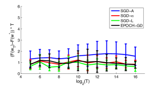
First, as a simple sanity check, we measured the performance of these algorithms on a simple, strongly convex stochastic optimization problem, which is also smooth. We define , and . The stochastic gradient oracle, given a point , returns the stochastic gradient where is uniformly distributed in . Clearly, this is an unbiased estimate of the gradient of at . The initial point of all 4 algorithms was chosen uniformly at random from . The results are presented in Fig. 1, and it is clear that all 4 algorithms indeed achieve a rate, matching our theoretical analysis (Thm. 1, Thm. 2 and Thm. 5). The results also seem to indicate that Sgd-A has a somewhat worse performance in terms of leading constants.
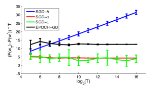
Second, as another simple experiment, we measured the performance of the algorithms on the non-smooth, strongly convex problem described in the proof of Thm. 4. In particular, we simulated this problem with , and picked uniformly at random from . The results are presented in Fig. 2. As our theory indicates, Sgd-A seems to have an convergence rate, whereas the other 3 algorithms all seem to have the optimal convergence rate. Among these algorithms, the SGD variants Sgd-L and Sgd- seem to perform somewhat better than Epoch-Gd. Also, while the average performance of Sgd-L and Sgd- are similar, Sgd- has less variance. This is reasonable, considering the fact that Sgd- returns an average of many points, whereas Sgd-L return only the very last point.
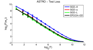
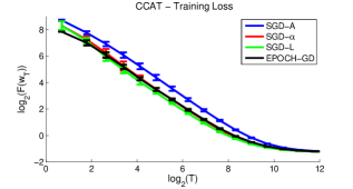
Finally, we performed a set of experiments on real-world data. We used the same 3 binary classification datasets (ccat,cov1 and astro-ph) used by Shalev-Shwartz et al. (2011) and Joachims (2006), to test the performance of optimization algorithms for Support Vector Machines using linear kernels. Each of these datasets is composed of a training set and a test set. Given a training set of instance-label pairs, , we defined to be the standard (non-smooth) objective function of Support Vector Machines, namely
| (4) |
Following Shalev-Shwartz et al. (2011) and Joachims (2006), we took for ccat, for cov1, and for astro-ph. The stochastic gradient given was computed by taking a single randomly drawn training example , and computing the gradient with respect to that example, namely
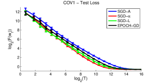
Each dataset comes with a separate test set, and we also report the objective function value with respect to that set (as in Eq. (4), this time with representing the test set examples). All algorithms were initialized at , with (i.e. no projections were performed - see the discussion in Sec. 2).
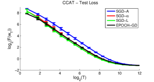
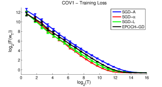
The results of the experiments are presented in Fig. 3,Fig. 4 and Fig. 5. In all experiments, Sgd-A performed the worst. The other 3 algorithms performed rather similarly, with Sgd- being slightly better on the Cov1 dataset, and Sgd-L being slightly better on the other 2 datasets.

In summary, our experiments indicate the following:
-
•
Sgd-A, which averages over all predictors, is worse than the other approaches. This accords with our theory, as well as the results reported in Shalev-Shwartz et al. (2011).
-
•
The Epoch-Gd algorithm does have better performance than Sgd-A, but a similar or better performance was obtained using the simpler approaches of -suffix averaging (Sgd-) or even just returning the last predictor (Sgd-L). The good performance of Sgd- is supported by our theoretical results, and so does the performance of Sgd-L in the strongly convex and smooth case.
-
•
Sgd-L also performed rather well (with what seems like a rate) on the non-smooth problem reported in Fig. 2, although with a larger variance than Sgd-. Our current theory does not cover the convergence of the last predictor in non-smooth problems - see the discussion below.
8 Discussion
In this paper, we analyzed the behavior of SGD for strongly convex stochastic optimization problems. We demonstrated that this simple and well-known algorithm performs optimally whenever the underlying function is smooth, but the standard averaging step can make it suboptimal for non-smooth problems. However, a simple modification of the averaging step suffices to recover the optimal rate, and a more sophisticated algorithm is not necessary. Our experiments seem to support this conclusion.
There are several open issues remaining. In particular, the rate in the non-smooth case still requires some sort of averaging. However, in our experiments and other studies (e.g. Shalev-Shwartz et al. (2011)), returning the last iterate also seems to perform quite well. Our current theory does not cover this - at best, one can use Lemma 1 and Jensen’s inequality to argue that the last iterate has a rate, but the behavior in practice is clearly much better. Does SGD, without averaging, obtain an rate for general strongly convex problems? Also, a fuller empirical study is warranted of whether and which averaging scheme is best in practice.
Acknowledgements: We thank Elad Hazan and Satyen Kale for helpful comments, and to Simon Lacoste-Julien for pointing out a bug in Lemma 1 in a previous version of this paper.
References
- Bach & Moulines (2011) Bach, F. and Moulines, E. Non-asymptotic analysis of stochastic approximation algorithms for machine learning. In NIPS, 2011.
- Bartlett et al. (2008) Bartlett, P.L., Dani, V., Hayes, T., Kakade, S., Rakhlin, A., and Tewari, A. High-probability regret bounds for bandit online linear optimization. In COLT, 2008.
- De La Peña (1999) De La Peña, V.H. A general class of exponential inequalities for martingales and ratios. The Annals of Probability, 27(1):537–564, 1999.
- Hazan & Kale (2011) Hazan, E. and Kale, S. Beyond the regret minimization barrier: An optimal algorithm for stochastic strongly-convex optimization. In COLT, 2011.
- Hazan et al. (2007) Hazan, E., Agarwal, A., and Kale, S. Logarithmic regret algorithms for online convex optimization. Machine Learning, 69(2-3):169–192, 2007.
- Joachims (2006) Joachims, T. Training linear SVMs in linear time. In KDD, 2006.
-
Juditsky & Nesterov (2010)
Juditsky, A. and Nesterov, Y.
Primal-dual subgradient methods for minimizing uniformly convex
functions.
Technical Report (August 2010), available at
http://hal.archives-ouvertes.fr/docs/00/50
/89/33/PDF/Strong-hal.pdf, 2010. - Kushner & Yin (2003) Kushner, H. and Yin, G. Stochastic Approximation and Recursive Algorithms and Applications. Springer, 2nd edition, 2003.
- Nemirovski et al. (2009) Nemirovski, A., Juditsky, A., Lan, G., and Shapiro, A. Robust stochastic approximation approach to stochastic programming. SIAM J. Optim., 19(4):1574–1609, 2009.
- Shalev-Shwartz et al. (2009) Shalev-Shwartz, S., Shamir, O., Srebro, N., and Sridharan, K. Stochastic convex optimization. In COLT, 2009.
- Shalev-Shwartz et al. (2011) Shalev-Shwartz, S., Singer, Y., Srebro, N., and Cotter, A. Pegasos: primal estimated sub-gradient solver for svm. Mathematical Programming, 127(1):3–30, 2011.
Appendix A Justifying Step-Sizes
In this appendix, we justify our focus on the step-size regime , by showing that for other step sizes, one cannot hope for an optimal convergence rate in general.
Let us begin by considering the scalar, strongly convex function , in the deterministic case where with probability , and show that cannot be smaller than . Intuitively, such small step sizes do not allow the iterates to move towards the optimum sufficiently fast. More formally, starting from (say) and using the recursive equality , we immediately get . Thus, if we want to obtain a convergence rate using the iterates returned by the algorithm, we must at least require that
This is equivalent to requiring that
For large enough and small enough , , and we get that must scale at least logarithmically with . This requires .
To show that cannot be larger than , one can consider the function over the domain - this is a one-dimensional special case of the example considered in Thm. 3. Intuitively, with an appropriate stochastic gradient model, the random fluctuations in (conditioned on ) are of order , so we need to get optimal rates. In particular, in the proof of Thm. 3, we show that for an appropriate stochastic gradient model, (see Eq. (B.4)). A similar lower bound can also be shown for the unconstrained setting considered in Thm. 4.
Appendix B Proofs
B.1 Some Technical Results
In this subsection we collect some technical Results we will need for the other proofs.
Lemma 2.
If , then
Proof.
Intuitively, the lemma holds because the strong convexity of implies that the expected value of must strictly increase as we get farther from . More precisely, strong convexity implies that for any ,
so by the Cauchy-Schwartz inequality,
| (5) |
Also, we have that
Combining this and Eq. (5), we get that for all ,
∎
The following version of Freedman’s inequality appears in De La Peña (1999) (Theorem 1.2A):
Theorem 6.
Let be a martingale difference sequence with a uniform upper bound on the steps . Let denote the sum of conditional variances,
Then, for every ,
The proof of the following lemma is taken almost verbatim from Bartlett et al. (2008), with the only modification being the use of Theorem 6 to avoid an unnecessary union bound.
Lemma 3.
Let be a martingale difference sequence with a uniform bound for all . Let be the sum of conditional variances of ’s. Further, let . Then we have, for any and ,
| (6) |
Proof.
Note that a crude upper bound on is . Thus, . We choose a discretization such that for and . We will specify the choice of shortly. We then have,
where the last inequality follows from Theorem 6. If we now choose , then for all . Hence every term in the above summation is bounded by . Choosing ensures that . Thus we have
∎
B.2 Proof of Lemma 1
By the strong convexity of and the fact that minimizes in , we have
as well as
Also, by convexity of , for any point and any we have . Using these inequalities, we have the following:
Plugging in , we get
By Lemma 2, we know that for , and the inequality above implies that for . The result now follows from a simple induction argument, using as the base case.
B.3 Proof of Thm. 2
For any , define . Then we have
Using the inequality for any random variables (which follows from Cauchy-Schwartz), and the bound of Lemma 1, we get that
By an induction argument (using Lemma 2 for the base case), it is easy to verify that
By the assumed smoothness of with respect to , we have . Combining it with the inequality above, the result follows.
B.4 Proof of Thm. 3
The SGD iterate can be written separately for the first coordinate as
| (7) |
Fix some , and suppose first that . Conditioned on this event, we have
since implies . On the other hand, if , we are still guaranteed that by the domain constraints. Using these results, we get
| (8) |
Therefore,
Thus, by definition of ,
Substituting gives the required result.
B.5 Proof of Thm. 4
The SGD iterate for the first coordinate is
| (9) |
The intuition of the proof is that whenever becomes negative, then the large gradient of causes to always be significantly larger than . This means that in some sense, is “constrained” to be larger than , mimicking the actual constraint in the example of Thm. 3 and forcing the same kind of behavior, with a resulting rate.
To make this intuition rigorous, we begin with the following lemma, which shows that can never be significantly smaller than , or “stay” below for more than one iteration.
Lemma 4.
For any , it holds that
and if , then
Proof.
Suppose first that . Then by Eq. (9) and the fact that , we get . Moreover, in that case, if , then by Eq. (9) and the previous observation,
Since , we have , which implies that the above is lower bounded by
Moreover, since , we have , so the projection operator is unnecessary, and we get overall that
This result was shown to hold assuming that . If , then repeating the argument above for instead of , we must have , so the statement in the lemma holds also when . ∎
We turn to the proof of Thm. 4 itself. By Lemma 4, if , then implies , and moreover, . Therefore, we have the following, where the sums below are only over ’s which are between and :
| (10) |
Now, we claim that the probabilities above can be lower bounded by a constant. To see this, consider each such probability for , conditioned on the event . Using the fact that , we have
This probability is at most , since it asks for being constrained in an interval of size , whereas is uniformly distributed over , which is an interval of length . As a result, we get
From this, we can lower bound Eq. (10) as follows:
Now, by Lemma 4, for any realization of , the indicators cannot equal consecutively. Therefore, must always be at least . Plugging it in the equation above, we get the lower bound . Summing up, we have shown that
By the boundedness assumption on , we have333To analyze the case where is unbounded, one can replace this by a coarse bound on how much can change in the first iterations, since the step sizes are bounded and is essentially a constant anyway. , so
Overall, we get
Therefore,
as required.
B.6 Proof of Thm. 5
Proof.
Using the derivation as in the proof of Lemma 1, we can upper bound by
Extracting the inner product and summing over , we get
By convexity of , is lower bounded by
Substituting this lower bound into Eq. (B.6) and slightly rearranging the right hand side, we get that can be upper bounded by
Now, we invoke Lemma 1, which tells us that with any strongly convex , even non-smooth, we have . More specifically, we can upper bound the expression above by
In particular, since we take , we get
It can be shown that . Plugging it in and slightly simplifying, we get the desired bound. ∎
B.7 Proof of Proposition 1
To prove this proposition, we will first prove the two auxiliary results, which rewrite in a more explicit form and provide a loose uniform upper bound. We will use the notation to denote .
Lemma 5.
For all , it holds with probability that
Proof.
The proof is analogous to that of Lemma 2, using the stronger condition that (which follows from the assumption with probability ). Using strong convexity, we have
The lemma trivially holds for . Otherwise, divide both sides by , and the result follows. ∎
Lemma 6.
Under the conditions of Proposition 1, it holds for any that
Proof.
By the strong convexity of and the fact that minimizes in , we have
as well as
Also, by convexity of , for any point and any we have . Using these inequalities, we have the following:
| (11) | |||||
Unwinding this recursive inequality till , we get that for any ,
We now note that
and therefore
as well as
Plugging this back, we get the desired bound. ∎
With this result at hand, we are now in a position to prove our high probability bound. Denote . We have that the conditional expectation of , given previous rounds, is , and the conditional variance, by Cauchy-Schwartz and the easily verified fact that , is . By Lemma 6, for all ,
| (12) |
Considering the sum , we have that the sum of conditional variances satisfies
We also have the uniform bound
| (13) |
where the last upper bound is by Lemma 5.
We now apply Lemma 3 to the sum of martingale differences , and get that as long as and , then with probability at least , for all ,
Plugging this back into Eq. (12), we get that with probability at least , for all ,
What is left to do now is an induction argument, to show that for a suitably chosen value of . By Lemma 5, this certainly holds for if . To show the induction step, let us rewrite the displayed inequality above as
where and . By the induction hypothesis, for all . Therefore, to show that , it suffices to find a sufficiently large value of so that
Clearly, it is enough to require
Multiplying both sides by , switching sides, and using the fact that as well as is at most for any , it follows that should satisfy
Solving the quadratic inequality, we get that should satisfy
Taking the square of both sides and using the fact that , it is again sufficient that
Substituting in the values of , we get
Thus, if we take
the induction hypothesis holds. Also, recall that for the base case to hold, we also need to assume , but this automatically holds for the value of above (since we assume ). This gives us the required result.