Removing Gaussian Noise by Optimization of Weights in Non-Local Means

Abstract

A new image denoising algorithm to deal with the additive Gaussian white noise model is given. Like the non-local means method, the filter is based on the weighted average of the observations in a neighborhood, with weights depending on the similarity of local patches. But in contrast to the non-local means filter, instead of using a fixed Gaussian kernel, we propose to choose the weights by minimizing a tight upper bound of mean square error. This approach makes it possible to define the weights adapted to the function at hand, mimicking the weights of the oracle filter. Under some regularity conditions on the target image, we show that the obtained estimator converges at the usual optimal rate. The proposed algorithm is parameter free in the sense that it automatically calculates the bandwidth of the smoothing kernel; it is fast and its implementation is straightforward. The performance of the new filter is illustrated by numerical simulations.

Keywords:   Non-local means, image denoising, optimization weights, oracle, statistical estimation.

1 Introduction

We deal with the additive Gaussian noise model

$$Y(x)=f(x)+\varepsilon(x),\;x\in\mathbf{I,}$$ (1)

where $\mathbf{I}$ is a uniform $N\times N$ grid of pixels on the unit square, $Y=\left(Y\left(x\right)\right)_{x\in\mathbf{I}}$ is the observed image brightness, $f:[0,1]^{2}\rightarrow\mathbf{R}_{+}$ is an unknown target regression function and $\varepsilon=\left(\varepsilon\left(x\right)\right)_{x\in\mathbf{I}}$ are independent and identically distributed (i.i.d.) Gaussian random variables with mean $0$ and standard deviation $\sigma>0.$ Important denoising techniques for the model (1) have been developed in recent years, see for example Buades, Coll and Morel (2005 [1]), Kervrann (2006 [10]), Lou, Zhang, Osher and Bertozzi (2010 [14]), Polzehl and Spokoiny (2006 [17]), Garnett, Huegerich and Chui (2005 [8]), Cai, Chan, Nikolova (2008 [3]), Katkovnik, Foi, Egiazarian, and Astola ( 2010 [9]), Dabov, Foi, Katkovnik and Egiazarian (2006 [2]). A significant step in these developments was the introduction of the Non-Local Means filter by Buades, Coll and Morel [1] and its variants (see e.g. [10], [11], [14]). In these filters, the basic idea is to estimate the unknown image $f(x_{0})$ by a weighted average of the form

$$\widetilde{f}_{w}(x_{0})=\sum_{x\in\mathbf{I}}w(x)Y(x),$$ (2)

where $w=\left(w\left(x\right)\right)_{x\in\mathbf{I}}$ are some non-negative weights satisfying $\sum_{x\in\mathbf{I}}w(x)=1.$ The choice of the weights $w$ are based essentially on two criteria: a local criterion so that the weights are as a decreasing function of the distance to the estimated pixel, and a non-local criterion which gives more important weights to the pixels whose brightness is close to the brightness of the estimated pixel (see e.g. Yaroslavsky (1985 [25]) and Tomasi and Manduchi (1998 [23])). The non-local approach has been further completed by a fruitful idea which consists in attaching small regions, called data patches, to each pixel and comparing these data patches instead of the pixels themselves.

The methods based on the non-local criterion consist of a comparatively novel direction which is less studied in the literature. In this paper we shall address two problems related to this criterion.

The first problem is how to choose data depending on weights $w$ in (2) in some optimal way. Generally, the weights $w$ are defined through some priory fixed kernels, often the Gaussian one, and the important problem of the choice of the kernel has not been addressed so far for the non-local approach. Although the choice of the Gaussian kernel seems to show reasonable numerical performance, there is no particular reason to restrict ourselves only to this type of kernel. Our theoretical results and the accompanying simulations show that another kernel should be preferred. In addition to this, for the obtained optimal kernel we shall also be interested in deriving a locally adaptive rule for the bandwidth choice. The second problem that we shall address is the convergence of the obtained filter to the true image. Insights can be found in [1], [10], [11] and [13], however the problem of convergence of the Non-Local Means Filter has not been completely settled so far. In this paper, we shall give some new elements of the proof of the convergence of the constructed filter, thereby giving a theoretical justification of the proposed approach from the asymptotic point of view.

Our main idea is to produce a very tight upper bound of the mean square error

$$R\left(\widetilde{f}_{w}(x_{0})\right)=\mathbb{E}\left(\widetilde{f}_{w}(x_{0})-f(x_{0})\right)^{2}$$

in terms of the bias and variance and to minimize this upper bound in $w$ under the constraints $w\geq 0$ and $\sum_{x\in\mathbf{I}}w(x)=1.$ In contrast to the usual approach where a specific class of target functions is considered, here we give a bound of the bias depending only on the target function $f$ at hand, instead of using just a bound expressed in terms of the parameters of the class. We first obtain an explicit formula for the optimal weights $w^{\ast}$ in terms of the unknown function $f.$ In order to get a computable filter, we estimate $w^{\ast}$ by some adaptive weights $\widehat{w}$ based on data patches from the observed image $Y.$ We thus obtain a new filter, which we call Optimal Weights Filter. To justify theoretically our filter, we prove that it achieves the optimal rate of convergence under some regularity conditions on $f.$ Numerical results show that Optimal Weights Filter outperforms the typical Non-Local Means Filter, thus giving a practical justification that the optimal choice of the kernel improves the quality of the denoising, while all other conditions are the same.

We would like to point out that related optimization problems for non parametric signal and density recovering have been proposed earlier in Sacks and Ylvysaker (1978 [22]), Roll (2003 [19]), Roll and Ljung (2004 [20]), Roll, Nazin and Ljung (2005 [21]), Nazin, Roll, Ljung and Grama (2008 [15]). In these papers the weights are optimized over a given class of regular functions and thus depend only on some parameters of the class. This approach corresponds to the minimax setting, where the resulting minimax estimator has the best rate of convergence corresponding to the worst image in the given class of images. If the image happens to have better regularity than the worst one, the minimax estimator will exhibit a slower rate of convergence than expected. The novelty of our work is to find the optimal weights depending on the image $f$ at hand, which implicates that our Optimal Weights Filter automatically attains the optimal rate of convergence for each particular image $f.$ Results of this type are related to the ”oracle” concept developed in Donoho and Johnstone (1994 [6]).

Filters with data-dependent weights have been previously studied in many papers, among which we mention Polzehl and Spokoiny (2000 [18], 2003 [16], 2006 [17]), Kervrann (2006 [10] and 2007 [12]). Compared with these filters our algorithm is straightforward to implement and gives a quality of denoising which is close to that of the best recent methods (see Table 2). The weight optimization approach can also be applied with these algorithms to improve them. In particular, we can use it with recent versions of the Non-Local Means Filter, like the BM3D (see 2006 [2], 2007 [4, 5]); however this is beyond the scope of the present paper and will be done elsewhere.

The paper is organized as follows. Our new filter based on the optimization of weights in the introduction in Section 2 where we present the main idea and the algorithm. Our main theoretical results are presented in Section 3 where we give the rate of convergence of the constructed estimators. In Section 4, we present our simulation results with a brief analysis. Proofs of the main results are deferred to Section 5.

To conclude this section, let us set some important notations to be used throughout the paper. The Euclidean norm of a vector $x=\left(x_{1},...,x_{d}\right)\in\mathbf{R}^{d}$ is denoted by $\left\|x\right\|_{2}=\left(\sum_{i=1}^{d}x_{i}^{2}\right).$ The supremum norm of $x$ is denoted by $\|x\|_{\infty}=\sup_{1\leq i\leq d}\left|x_{i}\right|.$ The cardinality of a set $\mathbf{A}$ is denoted $\text{card}\,\mathbf{A}$. For a positive integer $N$ the uniform $N\times N$-grid of pixels on the unit square is defined by

$$\mathbf{I}=\left\{\frac{1}{N},\frac{2}{N},\cdots,\frac{N-1}{N},1\right\}^{2}.$$ (3)

Each element $x$ of the grid $\mathbf{I}$ will be called pixel. The number of pixels is $n=N^{2}.$ For any pixel $x_{0}\in\mathbf{I}$ and a given $h>0,$ the square window of pixels

$$\mathbf{U}_{x_{0},h}=\left\{x\in\mathbf{I:\;}\|x-x_{0}\|_{\infty}\leq h\right\}$$ (4)

will be called search window at $x_{0}.$ We naturally take $h$ as a multiple of $\frac{1}{N}$ ($h=\frac{k}{N}$ for some $k\in\{1,2,\cdots,N\}$). The size of the square search window $\mathbf{U}_{x_{0},h}$ is the positive integer number

$$M=nh^{2}=\mathrm{card\ }\mathbf{U}_{x_{0},h}.$$

For any pixel $x\in\mathbf{U}_{x_{0},h}$ and a given $\eta>0$ a second square window of pixels

$$\mathbf{V}_{x,\eta}=\left\{y\in\mathbf{I:\;}\|y-x\|_{\infty}\leq\eta\right\}$$ (5)

will be called for short a patch window at $x$ in order to be distinguished from the search window $\mathbf{U}_{x_{0},h}.$ Like $h$, the parameter $\eta$ is also taken as a multiple of $\frac{1}{N}$. The size of the patch window $\mathbf{V}_{x,\eta}$ is the positive integer

$$m=n\eta^{2}=\mathrm{card\ }\mathbf{V}_{x_{0},\eta}.$$

The vector $\mathbf{Y}_{x,\eta}=\left(Y\left(y\right)\right)_{y\in\mathbf{V}_{x,\eta}}$ formed by the the values of the observed noisy image $Y$ at pixels in the patch $\mathbf{V}_{x,\eta}$ will be called simply data patch at $x\in\mathbf{U}_{x_{0},h}.$ Finally, the positive part of a real number $a$ is denoted by $a^{+},$ that is

$$a^{+}=\left\{\begin{array}[]{cc}a&\text{if }a\geq 0,\\ 0&\text{if }a<0.\end{array}\right.$$

2 Construction of the estimator

Let $h>0$ be fixed. For any pixel $x_{0}\in\mathbf{I}$ consider a family of weighted estimates $\widetilde{f}_{h,w}(x_{0})$ of the form

$$\widetilde{f}_{h,w}(x_{0})=\sum_{x\in\mathbf{U}_{x_{0},h}}w(x)Y(x),$$ (6)

where the unknown weights satisfy

$$w(x)\geq 0\;\;\;\text{and\ \ \ }\sum_{x\in\mathbf{U}_{x_{0},h}}w(x)=1.$$ (7)

The usual bias plus variance decomposition of the mean square error gives

$$\mathbb{E}\left(\widetilde{f}_{h,w}(x_{0})-f(x_{0})\right)^{2}=Bias^{2}+Var,$$ (8)

with

$$Bias^{2}=\left(\sum_{x\in\mathbf{U}_{x_{0},h}}w(x)\left(f(x)-f(x_{0})\right)\right)^{2}\;\;\text{and\ \ }Var=\sigma^{2}\sum_{x\in\mathbf{U}_{x_{0},h}}w(x)^{2}.$$

The decomposition (8) is commonly used to construct asymptotically minimax estimators over some given classes of functions in the nonparametric function estimation. In order to highlight the difference between the approach proposed in the present paper and the previous work, suppose that $f$ belongs to the class of functions satisfying the Hölder condition $|f(x)-f(y)|\leq L\|x-y\|_{\infty}^{\beta},\,\,\,\forall x,\,y\in\mathbf{I}.$ In this case, it is easy to see that

$$\mathbb{E}\left(\widetilde{f}_{h,w}(x_{0})-f(x_{0})\right)^{2}\leq\left(\sum_{x\in\mathbf{U}_{x_{0},h}}w(x)L\left|x-x_{0}\right|^{\beta}\right)^{2}+\sigma^{2}\sum_{x\in\mathbf{U}_{x_{0},h}}w(x)^{2}.$$ (9)

Optimizing further the weights $w$ in the obtained upper bound gives an asymptotically minimax estimate with weights depending on the unknown parameters $L$ and $\beta$ (for details see [22]). With our approach the bias term $Bias^{2}$ will be bounded in terms of the unknown function $f$ itself. As a result we obtain some ”oracle” weights $w$ adapted to the unknown function $f$ at hand, which will be estimated further using data patches from the image $Y.$

First, we shall address the problem of determining the ”oracle” weights. With this aim denote

$$\rho_{f,x_{0}}\left(x\right)\equiv\left|f(x)-f(x_{0})\right|.$$ (10)

Note that the value $\rho_{f,x_{0}}\left(x\right)$ characterizes the variation of the image brightness of the pixel $x$ with respect to the pixel $x_{0}.$ From the decomposition (8), we easily obtain a tight upper bound in terms of the vector $\rho_{f,x_{0}}:$

$$\mathbb{E}\left(\widetilde{f}_{h}(x_{0})-f(x_{0})\right)^{2}\leq g_{\rho_{f,x_{0}}}(w),$$ (11)

where

$$g_{\rho_{f,x_{0}}}(w)=\left(\sum_{x\in\mathbf{U}_{x_{0},h}}w(x)\rho_{f,x_{0}}(x)\right)^{2}+\sigma^{2}\sum_{x\in\mathbf{U}_{x_{0},h}}w(x)^{2}.$$ (12)

From the following theorem we can obtain the form of the weights $w$ which minimize the function $g_{\rho_{f,x_{0}}}(w)$ under the constraints (7) in terms of the values $\rho_{f,x_{0}}\left(x\right).$ For the sake of generality, we shall formulate the result for an arbitrary non-negative function $\rho\left(x\right),$ $x\in\mathbf{U}_{x_{0},h}.$ Define the objective function

$$g_{\rho}(w)=\left(\sum_{x\in\mathbf{U}_{x_{0},h}}w(x)\rho(x)\right)^{2}+\sigma^{2}\sum_{x\in\mathbf{U}_{x_{0},h}}w(x)^{2}.$$ (13)

Introduce into consideration the strictly increasing function

$$M_{\rho}\left(t\right)=\sum_{x\in\mathbf{U}_{x_{0},h}}\rho(x)(t-\rho(x))^{+},\ \ \ t\geq 0.$$ (14)

Let $K_{\text{tr}}$ be the usual triangular kernel:

$$K_{\text{tr}}\left(t\right)=\left(1-\left|t\right|\right)^{+},\quad t\in\mathbb{R}^{1}.$$ (15)

Theorem 1

Assume that $\rho\left(x\right),$ $x\in\mathbf{U}_{x_{0},h}$, is a non-negative function. Then the unique weights which minimize $g_{\rho}(w)$ subject to (7) are given by

$$w_{\rho}(x)=\frac{K_{\text{tr}}(\frac{\rho(x)}{a})}{\sum\limits_{y\in\mathbf{U}_{x_{0},h}}K_{\text{tr}}(\frac{\rho(x)}{a})},\quad x\in\mathbf{U}_{x_{0},h},$$ (16)

where the bandwidth $a>0$ is the unique solution on $(0,\infty)$ of the equation

$$M_{\rho}\left(a\right)=\sigma^{2}.$$ (17)

Theorem 1 can be obtained from a result of Sacks and Ylvysaker [22]. The proof is deferred to Section 5.1.

Remark 2

The value of $a>0$ can be calculated as follows. We sort the set $\{\rho(x)\,|\,x\in\mathbf{U}_{x_{0},h}\}$ in the ascending order $0=\rho_{1}\leq\rho_{2}\leq\cdots\leq\rho_{M}<\rho_{M+1}=+\infty$, where $M=Card\,\mathbf{U}_{x_{0},h}$. Let

$$a_{k}=\frac{\sigma^{2}+\sum\limits_{i=1}^{k}\rho_{i}^{2}}{\sum\limits_{i=1}^{k}\rho_{i}},\quad 1\leq k\leq M,$$ (18)

and

$$k^{*}=\max\{1\leq k\leq M\,|\,a_{k}\geq\rho_{k}\}=\min\{1\leq k\leq M\,|\,a_{k}<\rho_{k}\}-1,$$ (19)

with the convention that $a_{k}=\infty$ if $\rho_{k}=0$ and that $\min\varnothing=M+1$. Then the solution $a>0$ of (17) can be expressed as $a=a_{k^{*}}$; moreover, $k^{*}$ is the unique integer $k\in\{1,\cdots,M\}$ such that $a_{k}\geq\rho_{k}$ and $a_{k+1}<\rho_{k+1}$ if $k<M$.

The proof of the remark is deferred to Section 5.2.

Let $x_{0}\in\mathbf{I.}$ Using the optimal weights given by Theorem 1, we first introduce the following non computable approximation of the true image, called ”oracle”:

$$f_{h}^{\ast}(x_{0})=\frac{\sum_{x\in\mathbf{U}_{x_{0},h}}K_{\text{tr}}(\frac{\rho_{f,x_{0}}\left(x\right)}{a})Y(x)}{\sum\limits_{y\in\mathbf{U}_{x_{0},h}}K_{\text{tr}}(\frac{\rho_{f,x_{0}}\left(x\right)}{a})},$$ (20)

where the bandwidth $a$ is the solution of the equation $M_{\rho_{f,x_{0}}}\left(a\right)=\sigma^{2}.$ A computable filter can be obtained by estimating the unknown function $\rho_{f,x_{0}}\left(x\right)$ and the bandwidth $a$ from the data as follows.

Let $h>0$ and $\eta>0$ be fixed numbers. For any $x_{0}\in\mathbf{I}$ and any $x\in\mathbf{U}_{x_{0},h}$ consider a distance between the data patches $\mathbf{Y}_{x,\eta}=\left(Y\left(y\right)\right)_{y\in\mathbf{V}_{x,\eta}}$ and $\mathbf{Y}_{x_{0},\eta}=\left(Y\left(y\right)\right)_{y\in\mathbf{V}_{x_{0},\eta}}$ defined by

$$d^{2}\left(\mathbf{Y}_{x,\eta},\mathbf{Y}_{x_{0},\eta}\right)=\frac{1}{m}\left\|\mathbf{Y}_{x,\eta}-\mathbf{Y}_{x_{0},\eta}\right\|_{2}^{2},$$

where $m=\mathrm{card\ }\mathbf{V}_{x,\eta}$, and $\left\|\mathbf{Y}_{x,\eta}-\mathbf{Y}_{x_{0},\eta}\right\|_{2}^{2}=\sum\limits_{x_{0}+z\in\mathbf{V}_{x_{0},\eta}}\left(Y(x+z)-Y(x_{0}+z)\right)^{2}$. Since Buades, Coll and Morel [1] the distance $d^{2}\left(\mathbf{Y}_{x,\eta},\mathbf{Y}_{x_{0},\eta}\right)$ is known to be a flexible tool to measure the variations of the brightness of the image $Y.$ As

$$Y(x+z)-Y(x_{0}+z)=f(x+z)-f(x_{0}+z)+\epsilon(x+z)-\epsilon(x_{0}+z)$$

we have

$$\mathbb{E}(Y(x+z)-Y(x_{0}+z))^{2}=(f(x+z)-f(x_{0}+z))^{2}+2\sigma^{2}.$$

If we use the approximation

$$(f(x+z)-f(x_{0}+z))^{2}\approx(f(x)-f(x_{0}))^{2}=\rho^{2}_{f,x_{0}}(x)$$

and the law of large numbers, it seems reasonable that

$$\rho^{2}_{f,x_{0}}(x)\approx d^{2}(\mathbf{Y}_{x,\eta},\mathbf{Y}_{x_{0},\eta})-2\sigma^{2}.$$

But our simulations show that a much better approximation is

$$\rho_{f,x_{0}}(x)\approx\widehat{\rho}_{x_{0}}(x)=\left(d(\mathbf{Y}_{x,\eta},\mathbf{Y}_{x_{0},\eta})-\sqrt{2}\sigma\right)^{+}.$$ (21)

The fact that $\widehat{\rho}_{x_{0}}(x)$ is a good estimator of $\rho_{f,x_{0}}$ will be justified by convergence theorems: cf. Theorems 4 and 5 of Section 3. Thus our Optimal Weights Filter is defined by

$$\widehat{f}(x_{0})=\widehat{f}_{h,\eta}(x_{0})=\frac{\sum_{x\in\mathbf{U}_{x_{0},h}}K_{\text{tr}}(\frac{\widehat{\rho}_{x_{0}}\left(x\right)}{\widehat{a}})Y(x)}{\sum\limits_{y\in\mathbf{U}_{x_{0},h}}K_{\text{tr}}(\frac{\widehat{\rho}_{x_{0}}\left(x\right)}{\widehat{a}})},$$ (22)

where the bandwidth $\widehat{a}>0$ is the solution of the equation $M_{\widehat{\rho}_{x_{0}}}\left(\widehat{a}\right)=\sigma^{2}$, which can be calculated as in Remark 2 (with $\rho(x)$ and $a$ replaced by $\widehat{\rho}_{x_{0}}(x)$ and $\widehat{a}$ respectively). We end this section by giving an algorithm for computing the filter (22). The input values of the algorithm are the image $Y\left(x\right),$ $x\in\mathbf{I}$ , the variance of the noise $\sigma$ and two numbers $m$ and $M$ representing the sizes of the patch window and the search window respectively.

Algorithm : Optimal Weights Filter

Repeat for each $x_{0}\in\mathbf{I}$

give an initial value of $\widehat{a}$: $\widehat{a}=1$ (it can be an arbitrary positive number).

compute $\{\widehat{\rho}_{x_{0}}(x)\,|\,x\in\mathbf{U}_{x_{0},h}\}$ by (21)

/compute the bandwidth $\widehat{a}$ at $x_{0}$

reorder $\{\widehat{\rho}_{x_{0}}(x)\,|\,x\in\mathbf{U}_{x_{0},h}\}$ as increasing sequence, say

$\widehat{\rho}_{x_{0}}(x_{1})\leq\widehat{\rho}_{x_{0}}(x_{2})\leq\cdots\leq\widehat{\rho}_{x_{0}}(x_{M})$

loop from $k=1$ to $M$

if $\sum_{i=1}^{k}\widehat{\rho}_{x_{0}}(x_{i})>0$

if $\frac{\sigma^{2}+\sum_{i=1}^{k}\widehat{\rho}_{x_{0}}^{2}(x_{i})}{\sum_{i=1}^{k}\widehat{\rho}_{x_{0}}(x_{i})}\geq\widehat{\rho}(x_{k})$ then $\widehat{a}=\frac{\sigma^{2}+\sum_{i=1}^{k}\widehat{\rho}_{x_{0}}^{2}(x_{i})}{\sum_{i=1}^{k}\widehat{\rho}_{x_{0}}(x_{i})}$

else quit loop

else continue loop

end loop

/compute the estimated weights $\widehat{w}$ at $x_{0}$

compute $\widehat{w}(x_{i})=\frac{K_{\text{tr}}(1-\widehat{\rho}_{x_{0}}(x_{i})/\widehat{a})^{+}}{\sum_{x_{i}\in\mathbf{U}_{x_{0},h}}K_{\text{tr}}(1-\widehat{\rho}_{x_{0}}(x_{i})/\widehat{a})^{+}}$

/compute the filter $\widehat{f}$ at $x_{0}$

compute $\widehat{f}(x_{0})=\sum_{x_{i}\in\mathbf{U}_{x_{0},h}}\widehat{w}(x_{i})Y(x_{i})$.

The proposed algorithm is computationally fast and its implementation is straightforward compared to more sophisticated algorithms developed in recent years. Notice that an important issue in the non-local means filter is the choice of the bandwidth parameter in the Gaussian kernel; our algorithm is parameter free in the sense that it automatically chooses the bandwidth.

The numerical simulations show that our filter outperforms the classical non-local means filter under the same conditions. The overall performance of the proposed filter compared to its simplicity is very good which can be a big advantage in some practical applications. We hope that optimal weights that we deduced can be useful with more complicated algorithms and can give similar improvements of the denoising quality. However, these investigations are beyond the scope of the present paper. A detailed analysis of the performance of our filter is given in Section 4.

3 Main results

In this section, we present two theoretical results.

The first result is a mathematical justification of the ”oracle” filter introduced in the previous section. It shows that despite the fact that we minimized an upper bound of the mean square error instead of the mean square error itself, the obtained ”oracle” still has the optimal rate of convergence. Moreover, we show that the weights optimization approach possesses the following important adaptivity property: our procedure automatically chooses the correct bandwidth $a>0$ even if the radius $h>0$ of the search window $U_{x_{0},h}$ is larger than necessary.

The second result shows the convergence of the Optimal Weights Filter $\widehat{f}_{h,\eta}$ under some more restricted conditions than those formulated in Section 2. To prove the convergence, we split the image into two independent parts. From the first one, we construct the ”oracle” filter; from the second one, we estimate the weights. Under some regularity assumptions on the target image we are able to show that the resulting filter has nearly the optimal rate of convergence.

Let $\rho\left(x\right),$ $x\in\mathbf{U}_{x_{0},h},$ be an arbitrary non-negative function and let $w_{\rho}$ be the optimal weights given by (16). Using these weights $w_{\rho}$ we define the family of estimates

$$f_{h}^{\ast}(x_{0})=\sum_{x\in\mathbf{U}_{x_{0},h}}w_{\rho}(x)Y(x)$$ (23)

depending on the unknown function $\rho.$ The next theorem shows that one can pick up a useful estimate from the family $f_{h}^{\ast}$ if the the function $\rho$ is close to the ”true” function $\rho_{f,x_{0}}(x)=\left|f\left(x\right)-f\left(x_{0}\right)\right|,$ i.e. if

$$\rho\left(x\right)=\left|f\left(x\right)-f\left(x_{0}\right)\right|+\delta_{n},$$ (24)

where $\delta_{n}\geq 0$ is a small deterministic error. We shall prove the convergence of the estimate $f_{h}^{\ast}$ under the local Hölder condition

$$|f(x)-f(y)|\leq L\|x-y\|_{\infty}^{\beta},\,\,\,\forall x,\,y\in\mathbf{U}_{x_{0},h},$$ (25)

where $\beta>0$ is a constant, $h>0,$ and $x_{0}\in\mathbf{I}.$

In the following, $c_{i}>0$ $(i\geq 1)$ denotes a positive constant, and $O(a_{n})$ $(n\geq 1)$ denotes a number bounded by $c\cdot a_{n}$ for some constant $c>0$. All the constants $c_{i}>0$ and $c>0$ depend only on $L$, $\beta$ and $\sigma$; their values can be different from line to line.

Theorem 3

Assume that $h=c_{1}n^{-\frac{1}{2\beta+2}}$ with $c_{1}>c_{0}=\left(\frac{\sigma^{2}\left(\beta+2\right)\left(2\beta+2\right)}{8L^{2}\beta}\right)^{\frac{1}{2\beta+2}}$, or $h\geq c_{1}n^{-\alpha}$ with $0\leq\alpha<\frac{1}{2\beta+2}$ and $c_{1}>0$. Suppose that $f$ satisfies the local Hölder’s condition (25) and that $\delta_{n}=O\left(n^{-\frac{\beta}{2+2\beta}}\right).$ Then

$$\mathbb{E}\left(f_{h}^{\ast}(x_{0})-f(x_{0})\right)^{2}=O\left(n^{-\frac{2\beta}{2+2\beta}}\right).$$ (26)

The proof will be given in Section 5.3.

Recall that the bandwidth $h$ of order $n^{-\frac{1}{2+2\beta}}$ is required to have the optimal minimax rate of convergence $O\left(n^{-\frac{2\beta}{2+2\beta}}\right)$ of the mean squared error for estimating the function $f$ of global Hölder smoothness $\beta$ (cf. e.g. [7]). To better understand the adaptivity property of the oracle $f_{h}^{\ast}(x_{0}),$ assume that the image $f$ at $x_{0}$ has Hölder smoothness $\beta$ (see [24]) and that $h\geq c_{0}n^{-\alpha}$ with $0\leq\alpha<\frac{1}{2\beta+2},$ which means that the radius $h>0$ of the search window $U_{x_{0},h}$ has been chosen larger than the ”standard” $n^{-\frac{1}{2\beta+2}}.$ Then, by Theorem 3, the rate of convergence of the oracle is still of order $n^{-\frac{\beta}{2+2\beta}},$ contrary to the global case mentioned above. If we choose a sufficiently large search window $U_{x_{0},h},$ then the oracle $f_{h}^{\ast}(x_{0})$ will have a rate of convergence which depends only on the unknown maximal local smoothness $\beta$ of the image $f.$ In particular, if $\beta$ is very large, then the rate will be close to $n^{-1/2},$ which ensures good estimation of the flat regions in cases where the regions are indeed flat. More generally, since Theorem 3 is valid for arbitrary $\beta,$ it applies for the maximal local Hölder smoothness $\beta_{x_{0}}$ at $x_{0},$ therefore the oracle $f_{h}^{\ast}(x_{0})$ will exhibit the best rate of convergence of order $n^{-\frac{2\beta_{x_{0}}}{2+2\beta_{x_{0}}}}$ at $x_{0}.$ In other words, the procedure adapts to the best rate of convergence at each point $x_{0}$ of the image.

We justify by simulation results that the difference between the oracle $f_{h}^{\ast}$ computed with $\rho=\rho_{f,x_{0}}=\left|f\left(x\right)-f\left(x_{0}\right)\right|,$ and the true image $f$, is extremely small (see Table 1). This shows that, at least from the practical point of view, it is justified to optimize the upper bound $g_{\rho_{f,x_{0}}}(w)$ instead of optimizing the mean square error $\mathbb{E}\left(f^{\ast}_{h}(x_{0})-f(x_{0})\right)^{2}$ itself.

The estimate $f_{h}^{*}$ with the choice $\rho\left(x\right)=\rho_{f,x_{0}}\left(x\right)$ will be called oracle filter. In particular for the oracle filter $f_{h}^{\ast},$ under the conditions of Theorem 3, we have

$$\mathbb{E}\left(f_{h}^{\ast}(x_{0})-f(x_{0})\right)^{2}\leq g_{\rho}\left(w_{\rho}\right)\leq cn^{-\frac{2\beta}{2+2\beta}}.$$

Now, we turn to the study of the convergence of the Optimal Weights Filter. Due to the difficulty in dealing with the dependence of the weights we shall consider a slightly modified version of the proposed algorithm: we divide the set of pixels into two independent parts, so that the weights are constructed from the one part, and the estimation of the target function is a weighted mean along the other part. More precisely, assume that $x_{0}\in\mathbf{I},$ $h>0$ and $\eta>0.$ To prove the convergence we split the set of pixels into two parts $\mathbf{I}=\mathbf{I}_{x_{0}}^{\prime}\cup\mathbf{I}_{x_{0}}^{\prime\prime},$ where

$$\mathbf{I}_{x_{0}}^{\prime}=\left\{x_{0}+\left(\frac{i}{N},\frac{j}{N}\right)\in\mathbf{I}:i+j\text{ is even }\right\}$$ (27)

is the set of pixels with an even sum of coordinates $i+j$ and $\mathbf{I}_{x_{0}}^{\prime\prime}=\mathbf{I}\diagdown\mathbf{I}_{x_{0}}^{\prime}.$ Denote $\mathbf{U}_{x_{0},h}^{\prime}=\mathbf{U}_{x_{0},h}\cap\mathbf{I}_{x_{0}}^{\prime}$ and $\mathbf{V}_{x,\eta}^{\prime\prime}=\mathbf{V}_{x,\eta}\cap\mathbf{I}_{x_{0}}^{\prime\prime}.$ Consider the distance between the data patches $\mathbf{Y}_{x,\eta}^{\prime\prime}=\left(Y\left(y\right)\right)_{y\in\mathbf{V}_{x,\eta}^{\prime\prime}}$ and $\mathbf{Y}_{x_{0},\eta}^{\prime\prime}=\left(Y\left(y\right)\right)_{y\in\mathbf{V}_{x_{0},\eta}^{\prime\prime}}$ defined by

$$d\left(\mathbf{Y}_{x,\eta}^{\prime\prime},\mathbf{Y}_{x_{0},\eta}^{\prime\prime}\right)=\frac{1}{\sqrt{m^{\prime\prime}}}\left\|\mathbf{Y}_{x,\eta}^{\prime\prime}-\mathbf{Y}_{x_{0},\eta}^{\prime\prime}\right\|_{2},$$

where $m^{\prime\prime}=\mathrm{card\ }\mathbf{V}_{x,\eta}^{\prime\prime}.$ An estimate of the function $\rho_{f,x_{0}}$ is given by

$$\rho_{f,x_{0}}\left(x\right)\approx\widehat{\rho}_{x_{0}}^{\prime\prime}\left(x\right)=\left(d\left(\mathbf{Y}_{x,\eta}^{\prime\prime},\mathbf{Y}_{x_{0},\eta}^{\prime\prime}\right)-\sqrt{2}\sigma\right)^{+},$$ (28)

see (21). Define the filter $\widehat{f}_{h,\eta}^{\prime}$ by

$$\widehat{f}_{h,\eta}^{\prime}(x_{0})=\sum_{x\in\mathbf{U}_{x_{0},h}^{\prime}}\widehat{w}^{\prime\prime}(x)Y(x),$$ (29)

where

$$\widehat{w}^{\prime\prime}=\arg\min_{w}\left(\sum_{x\in\mathbf{U}_{x_{0},h}^{\prime}}w(x)\widehat{\rho}^{\prime\prime}_{x_{0}}(x)\right)^{2}+\sigma^{2}\sum_{x\in\mathbf{U}_{x_{0},h}^{\prime}}w^{2}(x).$$ (30)

The next theorem gives a rate of convergence of the Optimal Weights Filter if the parameters $h>0$ and $\eta>0$ are chosen properly according to the local smoothness $\beta.$

Theorem 4

Assume that $h=c_{1}n^{-\frac{1}{2\beta+2}}$ with $c_{1}>c_{0}=\left(\frac{\sigma^{2}\left(\beta+2\right)\left(2\beta+2\right)}{8L^{2}\beta}\right)^{\frac{1}{2\beta+2}}$, and that $\eta=c_{2}n^{-\frac{1}{2\beta+2}}.$ Suppose that function $f$ satisfies the local Hölder condition (25). Then

$$\mathbb{E}\left(\widehat{f}_{h,\eta}^{\prime}(x_{0})-f(x_{0})\right)^{2}=O\left(n^{-\frac{2\beta}{2\beta+2}}\ln n\right).$$ (31)

For the proof of this theorem see Section 5.4.

Theorem 4 states that with the proper choices of the parameters $h$ and $\eta$, the mean square error of the estimator $\widehat{f}^{\prime}_{h,\eta}(x_{0})$ converges nearly at the rate $O(n^{-\frac{2\beta}{2\beta+2}})$ which is the usual optimal rate of convergence for a given Hölder smoothness $\beta>0$ (cf. e.g. [7]).

Simulation results show that the adaptive bandwidth $\widehat{a}$ provided by our algorithm depends essentially on the local properties of the image and does not depend much on the radius $h$ of the search window. These simulations, together with Theorem 3, suggest that the Optimal Weights Filter (22) can also be applied with larger $h,$ as is the case of the ”oracle” filter $f_{h}^{\ast}.$ The following theorem deals with the case where $h$ is large.

Theorem 5

Assume that $h=c_{1}n^{-\alpha}$ with $c_{1}>0,$ and $0<\alpha\leq\frac{1}{2\beta+2}$ and that $\eta=c_{2}n^{-\frac{1}{2\beta+2}}.$ Suppose that the function $f$ satisfies the local Hölder condition (25). Then

$$\mathbb{E}\left(\widehat{f}_{h,\eta}^{\prime}(x_{0})-f(x_{0})\right)^{2}=O\left(n^{-\frac{\beta}{2\beta+2}}\ln n\right).$$

For the proof of this theorem see Section 5.5. Note that in this case the obtained rate of convergence is not the usual optimal one, in contrast to Theorems 3 and 4, but we believe that this is the best rate that can be obtained for the proposed filter.

4 Numerical performance of the Optimal Weights Filter

The performance of the Optimal Weights Filter $\widehat{f}_{h,\eta}(x_{0})$ is measured by the usual Peak Signal-to-Noise Ratio (PSNR) in decibels (db) defined as

$$PSNR=10\log_{10}\frac{255^{2}}{MSE},\,\,\,MSE=\frac{1}{card\,\mathbf{I}}\sum\limits_{x\in\mathbf{I}}(f(x)-\widehat{f}_{h,\eta}(x))^{2},$$

where $f$ is the original image, and $\widehat{f}$ the estimated one.

In the simulations, we sometimes shall use the smoothed version of the estimate of brightness variation $d_{K}\left(\mathbf{Y}_{x,\eta},\mathbf{Y}_{x_{0},\eta}\right)$ instead of the non smoothed one $d\left(\mathbf{Y}_{x,\eta},\mathbf{Y}_{x_{0},\eta}\right).$ It should be noted that for the smoothed versions of the estimated brightness variation we can establish similar convergence results. The smoothed estimate $d_{K}\left(\mathbf{Y}_{x,\eta},\mathbf{Y}_{x_{0},\eta}\right)$ is defined by

$$d_{K}\left(\mathbf{Y}_{x,\eta},\mathbf{Y}_{x_{0},\eta}\right)=\frac{\left\|K\left(y\right)\cdot\left(\mathbf{Y}_{x,\eta}-\mathbf{Y}_{x_{0},\eta}\right)\right\|_{2}}{\sqrt{\sum_{y^{\prime}\in\mathbf{V}_{x_{0},\eta}}K(y^{\prime})}},$$

where $K$ are some weights defined on $\mathbf{V}_{x_{0},\eta}.$ The corresponding estimate of brightness variation $\rho_{f,x_{0}}\left(x\right)$ is given by

$$\widehat{\rho}_{K,x_{0}}(x)=\left({d_{K}\left(\mathbf{Y}_{x,\eta},\mathbf{Y}_{x_{0},\eta}\right)}-\sqrt{2}\sigma\right)^{+}.$$ (32)

With the rectangular kernel

$$K_{r}\left(y\right)=\left\{\begin{array}[]{ll}1,&y\in\mathbf{V}_{x_{0},\eta},\\ 0,&\text{otherwise,}\end{array}\right.$$ (33)

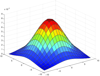
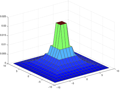
we obtain exactly the distance $d\left(\mathbf{Y}_{x,\eta},\mathbf{Y}_{x_{0},\eta}\right)$ and the filter described in Section 2. Other smoothing kernels $K$ used in the simulations are the Gaussian kernel

$$K_{g}(y)=\exp\left(-\frac{N^{2}\|y-x_{0}\|_{2}^{2}}{2h_{g}}\right),$$ (34)

where $h_{g}$ is the bandwidth parameter and the following kernel

$$K_{0}\left(y\right)=\left\{\begin{array}[]{ll}\sum_{k=N\left\|y-x_{0}\right\|_{\infty}}^{p}\frac{1}{(2k+1)^{2}}&\text{if }y\neq x_{0},\\ \sum_{k=1}^{p}\frac{1}{(2k+1)^{2}}&\text{if }y=x_{0},\end{array}\right.$$ (35)

with the width of the similarity window $m=(2p+1)^{2}.$ The shape of these two kernels are displayed in Figure 1.

To avoid the undesirable border effects in our simulations, we mirror the image outside the image limits, that is we extend the image outside the image limits symmetrically with respect to the border. At the corners, the image is extended symmetrically with respect to the corner pixels.

Images	Lena	Barbara	Boat	House	Peppers
Sizes	$512\times 512$	$512\times 512$	$512\times 512$	$256\times 256$	$256\times 256$
$\sigma/PSNR$	10/28.12db	10/28.12db	10/28.12db	10/28.11db	10/28.11db
$11\times 11$	41.20db	40.06db	40.23db	41.50db	40.36db
$13\times 13$	41.92db	40.82db	40.99db	42.24db	41.01db
$15\times 15$	42.54db	41.48db	41.62db	42.85db	41.53db
$17\times 17$	43.07db	42.05db	42.79db	43.38db	41.99db
$\sigma/PSNR$	20/22.11db	20/22.11db	20/22.11db	20/28.12db	20/28.12db
$11\times 11$	37.17db	35.92db	36.23db	37.18db	36.25db
$13\times 13$	37.91db	36.70db	37.01db	37.97db	36.85db
$15\times 15$	38.57db	37.37db	37.65db	38.59db	37.38db
$17\times 17$	39.15db	37.95db	38.22db	39.11db	37.80db
$\sigma/PSNR$	30/18.60db	30/18.60db	30/18.60db	30/18.61db	30/18.61db
$11\times 11$	34.81db	33.65db	33.79db	34.93db	33.57db
$13\times 13$	35.57db	34.47db	34.58db	35.78db	34.23db
$15\times 15$	36.24db	35.15db	35.25db	36.48db	34.78db
$17\times 17$	36.79db	35.75db	35.84db	37.07db	35.26db

Table 1: PSNR values when oracle estimator $f_{h}^{\ast}$ is applied with different values of $M$.

Figure 1: The shape of the kernels $K_{g}$ (left) and $K_{0}$ (right) with $M=$ $21\times 21$.

We have done simulations on a commonly-used set of images available at http://decsai.
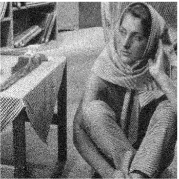
ugr.es/javier/denoise/test images/ which includes Lena, Barbara, Boat, House, Peppers. The potential of the estimation method is illustrated with the $512\times 512$ image ”Lena” (Figure 2(a)) and ”Barbara” (Figure  3(a) ) corrupted by an additive white Gaussian noise (Figures 2(b), PSNR$=22.10db$, $\sigma=20$ and  3 (b), PSNR$=18.60$, $\sigma=30$ ). We first used the rectangular kernel $K_{0}$ for computing the estimated brightness variation function $\widehat{\rho}_{K,x_{0}},$ which corresponds to the Optimal Weights Filter as defined in Section 2. 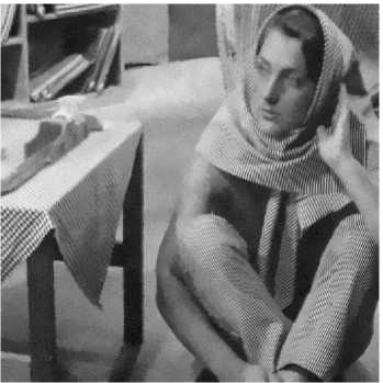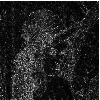Empirically we found that the parameters $m$ and $M$ can be fixed to $m=21\times 21$ and $M=13\times 13.$ In Figures 2(c) and  3(c), we can see that the noise is reduced in a natural manner and significant geometric features, fine textures, and original contrasts are visually well recovered with no undesirable artifacts (PSNR$=32.52db$ for ”Lena” and PSNR $=28.89$ for ”Barbara”). To better appreciate the accuracy of the restoration process, the square of the difference between the original image and the recovered image is shown in Figures 2(d) and  3(d), where the dark values correspond to a high-confidence estimate. 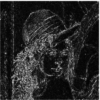As expected, pixels with a low level of confidence are located in the neighborhood of image discontinuities. For comparison, we show the image denoised by Non-Local Means Filter in Figures  2(e),(f) and  3 (e), (f). The overall visual impression and the numerical results are improved using our algorithm.

(a) Original image ”Lena”	(b) Noisy image with $\sigma=20$, $PSNR=22.11db$
(c) Restored with OWF, PSNR$=32.52db$	(d) Square error with OWF
(e) Restored with NLMF, PSNR$=31.73db$	(f) Square error with NLMF

Figure 2: Results of denoising ”Lena” $512\times 512$ image. Comparing (d) and (f) we see that the Optimal Weights Filter (OWF) captures more details than the Non-Local Means Filter (NLMF).

(a) Original image ”Barbara”	(b) Noisy image with $\sigma=30$, $PSNR=18.60db$
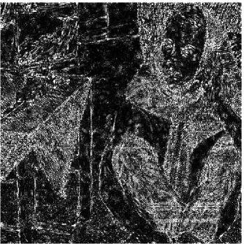(c) Restored with OWF, PSNR$=28.89db$	(d) Square error with OWF
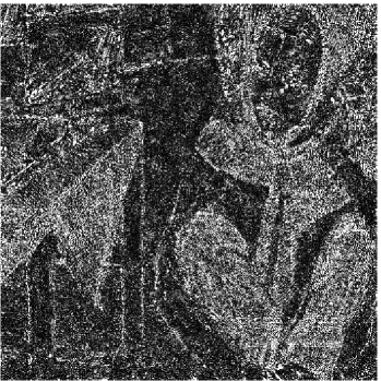(e) Restored with NLMF, PSNR$=27.88db$	(f) Square error with NLMF

Figure 3: Results of denoising ”Barbara” $512\times 512$ image. Comparing (d) and (f) we see that the Optimal Weights Filter (OWF) captures more details than the Non-Local Means Filter (NLMF).

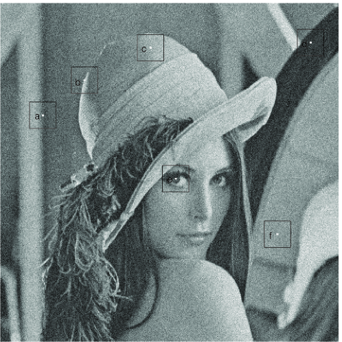
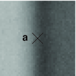
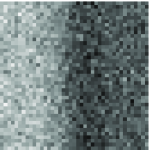
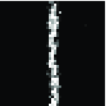
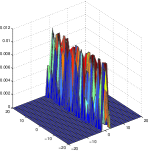
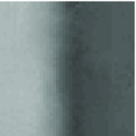
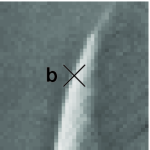
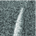
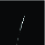
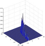
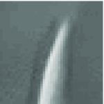
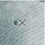
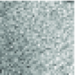
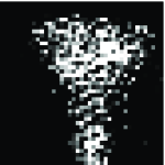
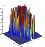
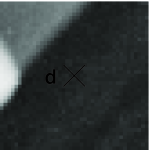
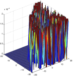
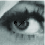
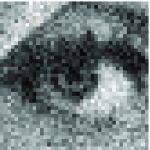
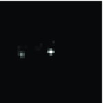
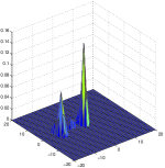
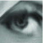
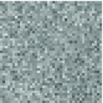
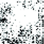
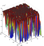
The Optimal Weights Filter seems to provide a feasible and rational method to detect automatically the details of images and take the proper weights for every possible geometric configuration of the image. For illustration purposes, we have chosen a series of search windows $\mathbf{U}_{x_{0},h}$ with centers at some testing pixels $x_{0}$ on the noisy image, see Figure 4 The distribution of the weights inside the search window $\mathbf{U}_{x_{0},h}$ depends on the estimated brightness variation function $\widehat{\rho}_{K,x_{0}}\left(x\right),$ $x\in\mathbf{U}_{x_{0},h}.$ If the estimated brightness variation $\widehat{\rho}_{K,x_{0}}\left(x\right)$ is less than $\widehat{a}$ (see Theorem 1), the similarity between pixels is measured by a linear decreasing function of $\widehat{\rho}_{K,x_{0}}\left(x\right);$ otherwise it is zero. Thus $\widehat{a}$ acts as an automatic threshold. In Figure 5, it is shown how the Optimal Weights Filter chooses in each case a proper weight configuration.

Figure 4: The noisy image with six selected search windows with centers at pixels a, b, c, d, e, f.

Original image	Noisy image	2D representation	3D representation	Restored image
		of the weights	of the weights

Figure 5: These pictures show how the Optimal Weights Filter detects the features of the image by choosing appropriate weights. The first column displays six selected search windows used to estimate the image at the corresponding central pixels a, b, c, d, e and f. The second column displays the corresponding search windows corrupted by a Gaussian noise with standard deviation $\sigma=20.$ The third column displays the two-dimensional representation of the weights used to estimate central pixels. The fourth column gives the three-dimensional representation of the weights. The fifth column gives the restored images.

The best numerical results are obtained using $K=K_{g}$ and $K=K_{0}$ in the definition of $\widehat{\rho}_{K,x_{0}}.$ In Table 2, we compare the Non-Local Mean Filter and the Optimal Weights filter with different choices of the kernel: $K=K_{g},K_{0},K_{r}.$ The best PSNR values we obtained by varying the size $m$ of the similarity windows and the size $M$ of the search windows are reported in Tables 3 ($\sigma=10$), 4 ($\sigma=20$) and 5 ($\sigma=30$) for $K=K_{0}.$ Note that the PSNR values are close for every $m$ and $M$ and the optimal $m$ and $M$ depend on the image content. The values $m=21\times 21$ and $M=13\times 13$ seem appropriate in most cases and a smaller patch size $m$ can be considered for processing piecewise smooth images.

Images	Lena	Barbara	Boat	House	Peppers
Sizes	$512\times 512$	$512\times 512$	$512\times 512$	$256\times 256$	$256\times 256$
$\sigma/PSNR$	10/28.12db	10/28.12db	10/28.12db	10/28.11db	10/28.11db
OWF with $K_{r}$	35.23db	33.89db	33.07db	35.57db	33.74db
OWF with $K_{g}$	35.49db	34.13db	33.40db	35.83db	33.97db
OWF with $K_{0}$	35.52db	34.10db	33.48db	35.80db	33.96db
NLMF	35.03db	33.77db	32.85db	35.43db	33.27db
$\sigma/PSNR$	20/22.11db	20/22.11db	20/22.11db	20/28.12db	20/28.12db
OWF with $K_{r}$	32.24db	30.71db	29.65db	32.59db	30.17db
OWF with $K_{g}$	32.61db	31.01db	30.05db	32.88db	30.44db
OWF with $K_{0}$	32.52db	31.00db	30.20db	32.90db	30.66db
NLMF	31.73db	30.36db	29.58db	32.51db	30.11db
$\sigma/PSNR$	30/18.60db	30/18.60db	30/18.60db	30/18.61db	30/18.61db
OWF with $K_{r}$	30.26db	28.59db	27.69db	30.49db	27.93db
OWF with $K_{g}$	30.66db	28.97db	28.05db	30.81db	28.16db
OWF with $K_{0}$	30.50db	28.89db	28.23db	30.80db	28.49db
NLMF	29.56db	27.88db	27.50db	30.02db	27.77db

Table 2: Comparison between the Non-Local Means Filter (NLMF) and the Optimal Weights Filter (OWF).

$\sigma=10$	Lena	Barbara	Boat	House	Peppers
$m/M$	$512\times 512$	$512\times 512$	$512\times 512$	$256\times 256$	$256\times 256$
$11\times 11/11\times 11$	35.35db	34.03db	33.43db	35.69db	34.16db
$13\times 13/11\times 11$	35.40db	34.06db	33.45db	35.72db	34.14db
$15\times 15/11\times 11$	35.44db	34.07db	33.47db	35.73db	34.10db
$17\times 17/11\times 11$	35.47db	34.08db	33.47db	35.74db	34.06db
$19\times 19/11\times 11$	35.50db	34.07db	33.48db	35.74db	34.02db
$21\times 21/11\times 11$	35.52db	34.06db	33.47db	35.73db	33.97db
$11\times 11/13\times 13$	35.35db	34.08db	33.43db	35.77db	34.15db
$13\times 13/13\times 13$	35.40db	34.11db	33.46db	35.79db	34.12db
$15\times 15/13\times 13$	35.44db	34.12db	33.47db	35.80db	34.09db
$17\times 17/13\times 13$	35.47db	34.12db	33.48db	35.81db	34.05db
$19\times 19/13\times 13$	35.50db	34.12db	33.48db	35.81db	34.01db
$21\times 21/13\times 13$	35.52db	34.10db	33.48db	35.80db	33.96db
$11\times 11/15\times 15$	35.33db	34.11db	33.43db	35.82db	34.14db
$13\times 13/15\times 15$	35.39db	34.13db	33.45db	35.84db	34.11db
$15\times 15/15\times 15$	35.43db	34.14db	33.47db	35.85db	34.08db
$17\times 17/15\times 15$	35.47db	34.14db	33.48db	35.86db	34.04db
$19\times 19/15\times 15$	35.49db	34.14db	33.48db	35.85db	34.00db
$21\times 21/15\times 15$	35.52db	34.12db	33.48db	35.84db	33.96db
$11\times 11/17\times 17$	35.32db	34.13db	33.42db	35.86db	34.12db
$13\times 13/17\times 17$	35.37db	34.15db	33.44db	35.88db	34.10db
$15\times 15/17\times 17$	35.42db	34.16db	33.46db	35.89db	34.07db
$17\times 17/17\times 17$	35.46db	34.16db	33.47db	35.89db	34.03db
$19\times 19/17\times 17$	35.48db	34.15db	33.47db	35.88db	34.00db
$21\times 21/17\times 17$	35.51db	34.14db	33.47db	35.87db	33.95db

Table 3: PSNR values when Optimal Weights Filter with $K=K_{0}$ is applied with different values of $m$ and $M$ ($\sigma=10$).

$\sigma=20$	Lena	Barbara	Boat	House	Peppers
$m/M$	$512\times 512$	$512\times 512$	$512\times 512$	$256\times 256$	$256\times 256$
$11\times 11/11\times 11$	32.08db	30.60db	30.00db	32.56db	30.65db
$13\times 13/11\times 11$	32.20db	30.70db	30.06db	32.64db	30.68db
$15\times 15/11\times 11$	32.30db	30.78db	30.11db	32.71db	30.70db
$17\times 17/11\times 11$	32.39db	30.84db	30.15db	32.76db	30.70db
$19\times 19/11\times 11$	32.47db	30.88db	30.18db	32.79db	30.70db
$21\times 21/11\times 11$	32.53db	30.91db	30.21db	32.81db	30.69db
$11\times 11/13\times 13$	32.06db	30.67db	29.99db	32.63db	30.61db
$13\times 13/13\times 13$	32.18db	30.78db	30.05db	32.71db	30.64db
$15\times 15/13\times 13$	32.29db	30.86db	30.10db	32.79db	30.66db
$17\times 17/13\times 13$	32.38db	30.92db	30.14db	32.84db	30.67db
$19\times 19/13\times 13$	32.46db	30.97db	30.18db	32.88db	30.67db
$21\times 21/13\times 13$	32.52db	31.00db	30.20db	32.90db	30.66db
$11\times 11/15\times 15$	32.02db	30.71db	29.97db	32.67db	30.56db
$13\times 13/15\times 15$	32.15db	30.82db	30.03db	32.76db	30.59db
$15\times 15/15\times 15$	32.26db	30.90db	30.08db	32.83db	30.62db
$17\times 17/15\times 15$	32.35db	30.96db	30.12db	32.89db	30.63db
$19\times 19/15\times 15$	32.43db	31.01db	30.16db	32.92db	30.63db
$21\times 21/15\times 15$	32.50db	31.04db	30.19db	32.94db	30.63db
$11\times 11/17\times 17$	31.97db	30.72db	29.94db	32.70db	30.52db
$13\times 13/17\times 17$	32.10db	30.83db	30.00db	32.79db	30.56db
$15\times 15/17\times 17$	32.22db	30.92db	30.05db	32.86db	30.58db
$17\times 17/17\times 17$	32.32db	30.98db	30.10db	32.92db	30.59db
$19\times 19/17\times 17$	32.40db	31.02db	30.13db	32.96db	30.60db
$21\times 21/17\times 17$	32.47db	31.06db	30.17db	32.98db	30.60db

Table 4: PSNR values when Optimal Weights Filter with $K=K_{0}$ is applied with different values of $m$ and $M$ ($\sigma=20$).

$\sigma=30$	Lena	Barbara	Boat	House	Peppers
$m/M$	$512\times 512$	$512\times 512$	$512\times 512$	$256\times 256$	$256\times 256$
$11\times 11/11\times 11$	29.96db	28.38db	27.96db	30.26db	28.36db
$13\times 13/11\times 11$	30.10db	28.53db	28.03db	30.39db	28.43db
$15\times 15/11\times 11$	30.23db	28.65db	28.10db	30.50db	28.47db
$17\times 17/11\times 11$	30.34db	28.75db	28.15db	30.58db	28.50db
$19\times 19/11\times 11$	30.43db	28.83db	28.20db	30.65db	28.51db
$21\times 21/11\times 11$	30.50db	28.81db	28.23db	30.70db	28.52db
$11\times 11/13\times 13$	29.94db	28.42db	27.95db	30.35db	28.30db
$13\times 13/13\times 13$	30.08db	28.58db	28.02db	30.49db	28.37db
$15\times 15/13\times 13$	30.21db	28.70db	28.09db	30.60db	28.42db
$17\times 17/13\times 13$	30.32db	28.80db	28.14db	30.68db	28.46db
$19\times 19/13\times 13$	30.42db	28.88db	28.19db	30.75db	28.48db
$21\times 21/13\times 13$	30.50db	28.89db	28.23db	30.80db	28.49db
$11\times 11/15\times 15$	29.89db	28.43db	27.92db	30.39db	28.23db
$13\times 13/15\times 15$	30.04db	28.58db	27.99db	30.53db	28.30db
$15\times 15/15\times 15$	30.17db	28.71db	28.06db	30.64db	28.36db
$17\times 17/15\times 15$	30.28db	28.81db	28.11db	30.73db	28.40db
$19\times 19/15\times 15$	30.38db	28.89db	28.16db	30.80db	28.43db
$11\times 11/17\times 17$	29.82db	28.40db	27.89db	30.39db	28.18db
$13\times 13/17\times 17$	29.98db	28.56db	27.96db	30.54db	28.26db
$15\times 15/17\times 17$	30.11db	28.69db	28.02db	30.66db	28.31db
$17\times 17/17\times 17$	30.22db	28.79db	28.08db	30.76db	28.36db
$19\times 19/17\times 17$	30.33db	28.87db	28.13db	30.84db	28.39db
$21\times 21/17\times 17$	30.42db	28.96db	28.17db	30.89db	28.41db

Table 5: PSNR values when Optimal Weights Filter with $K=K_{0}$ is applied with different values of $m$ and $M$ ($\sigma=30$).

5 Proofs of the main results

5.1 Proof of Theorem 1

We begin with some preliminary results. The following lemma can be obtained from Theorem 1 of Sacks and Ylvisaker [22]. For the convenience of readers, we prefer to give a direct proof adapted to our situation.

Lemma 6

Let $g_{\rho}(w)$ be defined by (13). Then there are unique weights $w_{\rho}$ which minimize $g_{\rho}(w)$ subject to (7), given by

$$w_{\rho}(x)=\frac{1}{\sigma^{2}}(b-\lambda\rho(x))^{+},$$ (36)

where $b$ and $\lambda$ are determined by

$$\sum_{x\in\mathbf{U}_{x_{0},h}}\frac{1}{\sigma^{2}}(b-\lambda\rho(x))^{+} = 1,$$ (37)

$$\sum_{x\in\mathbf{U}_{x_{0},h}}\frac{1}{\sigma^{2}}(b-\lambda\rho(x))^{+}\rho(x) = \lambda.$$ (38)

Proof. Let $w^{\prime}$ be a minimizer of $g_{\rho}\left(w\right)$ under the constraint (7). According to Theorem 3.9 of Whittle (1971 [24]), there are Lagrange multipliers $b\geq 0$ and $b_{0}(x)\geq 0,$ $x\in\mathbf{U}_{x_{0},h},$ such that the function

$$G(w)=g_{\rho}(w)-2b(\sum_{x\in\mathbf{U}_{x_{0},h}}w(x)-1)-2\sum_{x\in\mathbf{U}_{x_{0},h}}b_{0}(x)w(x)$$

is minimized at the same point $w^{\prime}.$ Since the function $G$ is strictly convex it admits a unique point of minimum. This implies that there is also a unique minimizer of $g_{\rho}\left(w\right)$ under the constraint (7) which coincides with the unique minimizer of $G.$

Let $w_{\rho}$ be the unique minimizer of $G$ satisfying the constraint (7). Again, using the fact that $G$ is strictly convex, for any $x\in\mathbf{U}_{x_{0},h},$

$$\frac{\partial}{\partial w\left(x\right)}G\left(w\right)\bigg{|}_{w=w_{\rho}}=2\left(\sum_{y\in\mathbf{U}_{x_{0},h}}w_{\rho}(y)\rho(y)\right)\rho(x)+2\sigma^{2}w_{\rho}(x)-2b-2b_{0}(x)\geq 0.$$ (39)

Note that in general we do not have an equality in (39). In addition, by the Karush-Kuhn-Tucker condition,

$$b_{0}(x)w_{\rho}(x)=0.$$ (40)

Let

$$\lambda=\sum_{y\in\mathbf{U}_{x_{0},h}}w_{\rho}(y)\rho(y).$$ (41)

Then (39) becomes

$$\frac{\partial}{\partial w\left(x\right)}G\left(w\right)\bigg{|}_{w=w_{\rho}}=\lambda\rho(x)+\sigma^{2}w_{\rho}(x)-b-b_{0}(x)\geq 0,\quad x\in\mathbf{U}_{x_{0},h}.$$ (42)

If $b_{0}(x)=0,$ then, with respect to the single variable $w(x)$ the function $G(w)$ attains its minimum at an interior point $w_{\rho}\left(x\right)\geq 0$, so that we have

$$\frac{\partial}{\partial w\left(x\right)}G\left(w\right)\bigg{|}_{w=w_{\rho}}=\lambda\rho(x)+\sigma^{2}w_{\rho}(x)-b=0.$$

From this we obtain $b-\lambda\rho(x)=\sigma w_{\rho}(x)\geq 0$, so

$$w_{\rho}(x)=\frac{(b-\lambda\rho(x))^{+}}{\sigma}.$$

If $b_{0}(x)>0$, by (40), we have $w_{\rho}(x)=0$. Consequently, from (42) we have

$$b-\lambda\rho(x)\leq-b_{0}(x)\leq 0,$$ (43)

so that we get again

$$w_{\rho}(x)=0=\frac{(b-\lambda\rho(x))^{+}}{\sigma}.$$

As to the conditions (37) and (38), they follow immediately from the constraint (7) and the equation (41).   

Proof of Theorem 1. Applying Lemma 6 with $b=\lambda a$, we see that the unique optimal weights $w$ minimizing $g_{\rho}(w)$ subject to (7), are given by

$$w_{\rho}=\frac{\lambda}{\sigma^{2}}(a-\rho(x))^{+},$$ (44)

where $a$ and $\lambda$ satisfy

$$\lambda\sum_{x\in\mathbf{U}_{x_{0},h}}(a-\rho(x))^{+}=\sigma^{2}$$ (45)

and

$$\sum_{x\in\mathbf{U}_{x_{0},h}}(a-\rho(x))^{+}\rho(x)=\sigma^{2}.$$ (46)

Since the function

$$M_{\rho}\left(t\right)=\sum_{x\in\mathbf{U}_{x_{0},h}}(t-\rho(x))^{+}\rho(x)$$

is strictly increasing and continuous with $M_{\rho}\left(0\right)=0$ and $\lim\limits_{t\rightarrow\infty}M_{\rho}\left(t\right)=+\infty,$ the equation

$$M_{\rho}\left(a\right)=\sigma^{2}$$

has a unique solution on $(0,\infty)$. By (45),

$$\frac{\sigma^{2}}{\lambda}=\sum_{x\in\mathbf{U}_{x_{0},h}}(a-\rho(x))^{+},$$

which together with (44) imply (16) and (17).

5.2 Proof of Remark 2

Expression (14) can be rewritten as

$$M_{\rho}(t)=\sum_{i=1}^{M}\rho_{i}(t-\rho_{i})^{+}.$$ (47)

Since function $M_{\rho}(t)$ is strictly increasing with $M_{\rho}(0)=0$ and $M_{\rho}(+\infty)=+\infty$, equation (17) admits a unique solution $a$ on $(0,+\infty)$, which must be located in some interval $[\rho_{k_{0}},\rho_{k_{0}+1})$, $1\leq k_{0}\leq M$, where $\rho_{M+1}=\infty$ (see Figure 6). Hence the equation (17) becomes

$$\sum_{i=1}^{k_{0}}\rho_{i}(a-\rho_{i})=\sigma^{2},$$ (48)

where $\quad\rho_{k_{0}}\leq a<\rho_{k_{0}+1}$. From (48), it follows that

$$a=\frac{\sigma^{2}+\sum\limits_{i=1}^{k_{0}}\rho_{i}^{2}}{\sum\limits_{i=1}^{k_{0}}\rho_{i}},\quad\rho_{k_{0}}\leq a<\rho_{k_{0}+1}.$$ (49)

We now show that $k_{0}=k^{*}$ (so that $a=k_{0}=k^{*}$), where $k^{*}:=\max\{1\leq k\leq M\,|\,a_{k}\geq\rho_{k}\}$. To this end, it suffices to verify that $a_{k_{0}}\geq\rho_{k_{0}}$ and $a_{k}<\rho_{k}$ if $k_{0}<k\leq M$. We have already seen that $a_{k_{0}}\geq\rho_{k_{0}}$; if $k_{0}<k\leq M$, then $a_{k_{0}}<\rho_{k_{0}+1}\leq\rho_{k}$, so that

$$a_{k}=\frac{(\sigma^{2}+\sum\limits_{i=1}^{k_{0}}\rho_{i}^{2})+\sum\limits_{i=k_{0}+1}^{k}\rho_{i}^{2}}{\sum\limits_{i=1}^{k}\rho_{i}}=\frac{a_{k_{0}}\sum\limits_{i=1}^{k_{0}}\rho_{i}+\sum\limits_{k_{0}+1}^{k}\rho_{i}^{2}}{\sum\limits_{i=1}^{k}\rho_{i}}<\frac{\rho_{k}\sum\limits_{i=1}^{k_{0}}\rho_{i}+\sum\limits_{k_{0}+1}^{k}\rho_{k}\rho_{i}}{\sum\limits_{i=1}^{k}\rho_{i}}=\rho_{k}.$$ (50)

We finally prove that if $1\leq k<M$ and $a_{k}<\rho_{k}$, then $a_{k+1}<\rho_{k+1}$, so that the last equality in (19) holds and that $k^{*}$ is the unique integer $k\in\{1,\cdots,M\}$ such that $a_{k}\geq\rho_{k}$ and $a_{k+1}<\rho_{k+1}$ if $1\leq k<M$. In fact, for $1\leq k<M$, the inequality $a_{k}<\rho_{k}$ implies that

$$\sigma^{2}+\sum_{i=1}^{k}\rho_{i}^{2}<\rho_{k}\sum_{i=1}^{k}\rho_{i}.$$

This, in turn, implies that

$$a_{k+1}=\frac{\sigma^{2}+\sum\limits_{i=1}^{k}\rho_{i}^{2}+\rho_{k+1}^{2}}{\sum\limits_{i=1}^{k+1}\rho_{i}}<\frac{\rho_{k}\sum\limits_{i=1}^{k}\rho_{i}+\rho_{k+1}^{2}}{\sum\limits_{i=1}^{k+1}\rho_{i}}\leq\rho_{k+1}.$$

Figure 6: The number axis of $\rho_{i}$, $i=1,2,\cdots,M$.

5.3 Proof of Theorem 3

First assume that $\rho\left(x\right)=\rho_{f,x_{0}}(x)=|f(x)-f(x_{0})|.$ Recall that $g_{\rho}$ and $w_{\rho}$ were defined by (13) and (16). Using Hölder’s condition (25) we have, for any $w$,

$$g_{\rho}(w_{\rho})\leq g_{\rho}(w)\leq\overline{g}(w),$$

where

$$\overline{g}(w)=\left(\sum_{x\in\mathbf{U}_{x_{0},h}}w(x)L\|x-x_{0}\|_{\infty}^{\beta}\right)^{2}+\sigma^{2}\sum_{x\in\mathbf{U}_{x_{0},h}}w^{2}(x).$$

In particular, denoting $\overline{w}=\arg\min_{w}\overline{g}(w),$ we get

$$g_{\rho}(w_{\rho})\leq\overline{g}(\overline{w}).$$

By Theorem 1,

$$\overline{w}(x)=\left(a-L\|x-x_{0}\|_{\infty}^{\beta}\right)^{+}\Big{/}\sum\limits_{y\in\mathbf{U}_{x_{0},h}}\left(a-L\|x-x_{0}\|_{\infty}^{\beta}\right)^{+},$$

where $a>0$ is the unique solution on $(0,\infty)$ of the equation $\overline{M}_{h}(a)=\sigma^{2}$, with

$$\overline{M}_{h}\left(t\right)=\sum_{x\in\mathbf{U}_{x_{0},h}}L\|x-x_{0}\|_{\infty}^{\beta}(t-L\|x-x_{0}\|_{\infty}^{\beta})^{+},\quad t\geq 0.$$

Theorem 3 will be a consequence of the following lemma.

Lemma 7

Assume that $\rho(x)=L\|x-x_{0}\|_{\infty}^{\beta}$ and that $h\geq c_{1}n^{-\alpha}$ with $0\leq\alpha<\frac{1}{2\beta+2}$, or $h=c_{1}n^{-\frac{1}{2\beta+2}}$ with $c_{1}>c_{0}=\left(\frac{\sigma^{2}(2\beta+2)(\beta+2)}{8L^{2}}\right)^{\frac{1}{2\beta+2}}.$ Then

$$a=c_{3}n^{-\beta/(2\beta+2)}(1+o(1))$$ (51)

and

$$\overline{g}(\overline{w})\leq c_{4}n^{-\frac{2\beta}{2+2\beta}},$$ (52)

where $c_{3}$ and $c_{4}$ are positive constants depending only on $\beta,$ $L$ and $\sigma.$

Proof. We first prove (51) in the case where $h=1$, i.e. $\mathbf{U}_{x_{0},h}=\mathbf{I}$. Then by the definition of $a,$ we have

$$\overline{M}_{1}\left(a\right)=\sum\limits_{x\in I}(a-L\|x-x_{0}\|_{\infty}^{\beta})^{+}L\|x-x_{0}\|_{\infty}^{\beta}=\sigma^{2}.$$ (53)

Let $\overline{h}=\left(a/L\right)^{1/\beta}$. Then $a-L\|x-x_{0}\|_{\infty}^{\beta}\geq 0$ if and only if $\|x-x_{0}\|_{\infty}\leq\overline{h}$. So from (53) we get

$$L^{2}\overline{h}^{\beta}\sum_{\|x-x_{0}\|_{\infty}\leq\overline{h}}\|x-x_{0}\|_{\infty}^{\beta}-L^{2}\sum_{\|x-x_{0}\|_{\infty}\leq\overline{h}}\|x-x_{0}\|_{\infty}^{2\beta}=\sigma^{2}.$$ (54)

By the definition of the neighborhood $U_{x_{0},\overline{h}}$ it is easily seen that

$$\sum_{\|x-x_{0}\|_{\infty}\leq\overline{h}}\|x-x_{0}\|_{\infty}^{\beta}=8N^{-\beta}\sum_{k=1}^{N\overline{h}}k^{\beta+1}=8N^{2}\frac{\overline{h}^{\beta+2}}{\beta+2}\left(1+o\left(1\right)\right)$$

and

$$\sum_{\|x-x_{0}\|_{\infty}\leq\overline{h}}\|x-x_{0}\|_{\infty}^{2\beta}=8N^{-2\beta}\sum_{k=1}^{N\overline{h}}k^{2\beta+1}=8N^{2}\frac{\overline{h}^{2\beta+2}}{2\beta+2}\left(1+o\left(1\right)\right).$$

Therefore, (54) implies

$$\frac{8L^{2}\beta}{\left(\beta+2\right)\left(2\beta+2\right)}N^{2}\overline{h}^{2\beta+2}(1+o{(1)})=\sigma^{2},$$

from which we infer that

$$\overline{h}=c_{0}n^{-\frac{1}{2\beta+2}}(1+o(1))$$ (55)

with $c_{0}=\left(\frac{\sigma^{2}\left(\beta+2\right)\left(2\beta+2\right)}{8L^{2}\beta}\right)^{\frac{1}{2\beta+2}}.$ From (55) and the definition of $\overline{h}$, we obtain

$$a=L\overline{h}^{\beta}=Lc_{0}^{\beta}n^{-\frac{\beta}{2\beta+2}}(1+o(1)),$$

which prove (51) in the case when $h=1$.

We next prove (51) under the conditions of the lemma. If $h\geq c_{0}n^{-\alpha},$ where $0\leq\alpha<\frac{1}{2\beta+2},$ then it is clear that $h\geq\overline{h}$ for $n$ sufficiently large. Therefore $\overline{M}_{h}\left(a\right)=\overline{M}_{1}\left(a\right)$, thus we arrive at equation (53) from which we deduce (55). If $h\geq c_{0}n^{-\frac{1}{2\beta+2}}$ and $c_{0}>c_{1},$ then again $h\geq\overline{h}$ for $n$ sufficiently large. Therefore $\overline{M}_{h}\left(a\right)=\overline{M}_{1}\left(a\right)$, and we arrive again at (55).

We finally prove (52). Denote for brevity

$$G_{h}=\sum_{\|x-x_{0}\|_{\infty}\leq h}(\overline{h}^{\beta}-\|x-x_{0}\|_{\infty}^{\beta})^{+}.$$

Since $h\geq\overline{h}$ for $n$ sufficiently large, we have $\overline{M}_{h}\left(a\right)=\overline{M}_{\overline{h}}\left(a\right)=\sigma^{2}$ and $G_{h}=G_{\overline{h}}.$ Then it is easy to see that

$$\overline{g}(\overline{w}) = \sigma^{2}\frac{\overline{M}_{\overline{h}}\left(a\right)+\sum_{\|x-x_{0}\|_{\infty}\leq\overline{h}}\left(\left(\overline{a}-L\|x-x_{0}\|_{\infty}^{\beta}\right)^{+}\right)^{2}}{L^{2}G_{\overline{h}}^{2}}$$

$$= \frac{\sigma^{2}}{L}\frac{a}{G_{\overline{h}}}.$$

Since

$$G_{h} =\sum_{\|x-x_{0}\|_{\infty}\leq\overline{h}}(\overline{h}^{\beta}-\|x-x_{0}\|_{\infty}^{\beta})$$

$$=\overline{h}^{\beta}\sum_{1\leq k\leq N\overline{h}}8k-\frac{8}{N^{\beta}}\sum_{1\leq k\leq N\overline{h}}k^{\beta+1}$$

$$=\frac{4\beta}{\beta+2}N^{2}\overline{h}^{\beta+2}\left(1+o\left(1\right)\right)$$

$$=\frac{4\beta}{\left(\beta+2\right)L^{1/\beta}}N^{2}a^{\left(\beta+2\right)/\beta}\left(1+o\left(1\right)\right),$$

we obtain

$$\overline{g}\left(\overline{w}\right)=\sigma^{2}\frac{\left(\beta+2\right)}{4\beta}L^{1/\beta-1}\frac{\overline{a}^{-\frac{2}{\beta}}}{N^{2}}\left(1+o\left(1\right)\right)=c_{5}n^{-\frac{2\beta}{2\beta+2}}\left(1+o\left(1\right)\right),$$

where $c_{4}$ is a constant depending on $\beta,$ $L$ and $\sigma.$   

Proof of Theorem 3. As $\rho\left(x\right)=\left|f\left(x\right)-f\left(x_{0}\right)\right|+\delta_{n},$ we have

$$\begin{split}\left(\sum_{x\in\mathbf{U}_{x_{0},h}}w(x)\rho(x)\right)^{2}&\leq\left(\sum_{x\in\mathbf{U}_{x_{0},h}}w(x)|f(x)-f(x_{0})|+\delta_{n}\right)^{2}\\ &\leq 2\left(\sum_{x\in\mathbf{U}_{x_{0},h}}w(x)|f(x)-f(x_{0})|\right)^{2}+2\delta_{n}^{2}.\end{split}$$

Hence

$$g_{\rho}(w)\leq 2\overline{g}(w)+2\delta_{n}^{2}.$$

So

$$g_{\rho}(w_{\rho})\leq g_{\rho}(\overline{w})\leq 2\overline{g}(\overline{w})+2\delta_{n}^{2}.$$

Therefore, by Lemma 7 and the condition that $\delta_{n}=O\left(n^{-\frac{\beta}{2\beta+2}}\right)$, we obtain

$$g_{\rho}(w_{\rho})=O\left(n^{-\frac{2\beta}{2\beta+2}}\right).$$

This gives (26).

5.4 Proof of Theorem 4

We begin with a decomposition of $\widehat{\rho}_{x_{0}}^{\prime\prime}(x)$. Note that

$$\widehat{\rho}_{x_{0}}^{\prime\prime}(x)=\left(d\left(\mathbf{Y}_{x,\eta}^{\prime\prime},\mathbf{Y}_{x_{0},\eta}^{\prime\prime}\right)-\sigma\sqrt{2}\right)^{+}\leq\left|d\left(\mathbf{Y}_{x,\eta}^{\prime\prime},\mathbf{Y}_{x_{0},\eta}^{\prime\prime}\right)-\sigma\sqrt{2}\right|.$$ (56)

Recall that $M^{\prime}=\mathrm{card\ }\mathbf{U}_{x_{0},h}^{\prime}=nh^{2}/2$, $m^{\prime\prime}=\mathrm{card\ }\mathbf{V}_{x_{0},\eta}^{\prime\prime}=n\eta^{2}/2.$ Let $T_{x_{0},x}$ be the translation mapping $T_{x_{0},x}y=x+(y-x_{0}).$ Denote $\Delta_{x_{0},x}\left(y\right)=f(y)-f(T_{x_{0},x}y)$ and $\zeta\left(y\right)=\varepsilon(y)-\varepsilon(T_{x_{0},x}y).$ Since

$$Y(y)-Y(T_{x_{0},x}y)=\Delta_{x_{0},x}\left(y\right)+\zeta\left(y\right),$$

it is easy to see that

$$d\left(\mathbf{Y}_{x,\eta}^{\prime\prime},\mathbf{Y}_{x_{0},\eta}^{\prime\prime}\right)^{2}=\frac{1}{m^{\prime\prime}}\sum_{y\in\mathbf{V}_{x_{0},\eta}^{\prime\prime}}\left(\Delta_{x_{0},x}\left(y\right)+\zeta\left(y\right)\right)^{2}=\Delta^{2}\left(x\right)+S\left(x\right)+2\sigma^{2},$$

where

$$\Delta^{2}\left(x\right) = \frac{1}{m^{\prime\prime}}\sum_{y\in\mathbf{V}_{x_{0},\eta}^{\prime\prime}}\Delta_{x_{0},x}^{2}\left(y\right),$$ (57)

$$S\left(x\right) = -2S_{1}\left(x\right)+S_{2}\left(x\right)$$ (58)

with

$$S_{1}(x) = \frac{1}{m^{\prime\prime}}\sum_{y\in\mathbf{V}_{x_{0},\eta}^{\prime\prime}}\Delta_{x_{0},x}\left(y\right)\zeta\left(y\right),$$

$$S_{2}(x) = \frac{1}{m^{\prime\prime}}\sum_{y\in\mathbf{V}_{x_{0},\eta}^{\prime\prime}}\left(\zeta\left(y\right)^{2}-2\sigma^{2}\right).$$

Notice that $\mathbb{E}S_{1}(x)=\mathbb{E}S_{2}\left(x\right)=\mathbb{E}S\left(x\right)=0.$ Then obviously

$$d\left(\mathbf{Y}_{x,\eta}^{\prime\prime},\mathbf{Y}_{x_{0},\eta}^{\prime\prime}\right)-\sigma\sqrt{2} = \sqrt{\Delta^{2}(x)+S\left(x\right)+2\sigma^{2}}-\sqrt{2\sigma^{2}}$$ (59)

$$= \frac{\Delta^{2}(x)+S(x)}{\sqrt{\Delta^{2}(x)+S\left(x\right)+2\sigma^{2}}+\sqrt{2\sigma^{2}}}.$$

First we prove the following lemma.

Lemma 8

Suppose that the function $f$ satisfies the local Hölder condition (25). Then, for any $x\in\mathbf{U}_{x_{0},h}^{\prime},$

$$\frac{1}{3}\rho_{f,x_{0}}^{2}\left(x\right)-2L^{2}\eta^{2\beta}\leq\Delta^{2}\left(x\right)\leq 3\rho_{f,x_{0}}^{2}\left(x\right)+6L^{2}\eta^{2\beta}.$$

Proof. By the decomposition

$$f\left(y\right)-f\left(T_{x_{0},x}\left(y\right)\right)=\left[f\left(x_{0}\right)-f\left(x\right)\right]+\left[f\left(y\right)-f\left(x_{0}\right)\right]+\left[f\left(x\right)-f\left(T_{x_{0},x}\left(y\right)\right)\right]$$

and the inequality $\left(a+b+c\right)^{2}\leq 3\left(a^{2}+b^{2}+c^{3}\right)$ we obtain

$$\Delta^{2}\left(x\right) = \frac{1}{m^{\prime\prime}}\sum_{y\in\mathbf{V}_{x_{0},\eta}^{\prime\prime}}\left(f\left(y\right)-f\left(T_{x_{0},x}\left(y\right)\right)\right)^{2}$$

$$\leq \frac{3}{m^{\prime\prime}}\sum_{y\in\mathbf{V}_{x_{0},\eta}^{\prime\prime}}\left(f\left(x_{0}\right)-f\left(x\right)\right)^{2}$$

$$\frac{3}{m^{\prime\prime}}\sum_{y\in\mathbf{V}_{x_{0},\eta}^{\prime\prime}}\left(f\left(y\right)-f\left(x_{0}\right)\right)^{2}$$

$$\frac{3}{m^{\prime\prime}}\sum_{y\in\mathbf{V}_{x_{0},\eta}^{\prime\prime}}\left(f\left(x\right)-f\left(T_{x_{0},x}\left(y\right)\right)\right)^{2}.$$

By the local Hölder condition (25) this implies

$$\Delta^{2}\left(x\right)\leq 3\left(f\left(x_{0}\right)-f\left(x\right)\right)^{2}+3L^{2}\eta^{2\beta}+3L^{2}\eta^{2\beta},$$

which gives the upper bound. The lower bound can be proved similarly using the inequality $\left(a+b+c\right)^{2}\geq\frac{1}{3}a^{2}-b^{2}-c^{2}.$   

We first prove a large deviation inequality for $S(x)$.

Lemma 9

Let $S(x)$ be defined by (58). Then there are two constants $c_{1}$ and $c_{2}$ such that for any $0\leq z\leq c_{1}\left(m^{\prime\prime}\right)^{1/2},$

$$\mathbb{P}\left(\left|S(x)\right|\geq\frac{z}{\sqrt{m^{\prime\prime}}}\right)\leq 2\exp\left(-c_{2}z^{2}\right).$$

Proof. Denote $\xi\left(y\right)=\zeta\left(y\right)^{2}-2\sigma^{2}-2\Delta_{x_{0},x}\left(y\right)\zeta\left(y\right).$ Since $\zeta\left(y\right)=\varepsilon(y)-\varepsilon(T_{x_{0},x}y)$ is a normal random variable with mean $0$ and variance $2\sigma^{2}$, the random variable $\xi\left(y\right)$ has an exponential moment, i.e. there exist two positive constants $t_{0}$ and $c_{3}$ depending only on $\beta,$ $L$ and $\sigma^{2}$ such that $\phi_{y}\left(t\right)=\mathbb{E}e^{t\xi(y)}\leq c_{3},$ for any $\left|t\right|\leq t_{0}.$ Let $\psi_{y}(t)=\ln\phi_{y}\left(t\right)$ be the cumulate generating function. By Chebyshev’s exponential inequality we get,

$$\mathbb{P}\{S(x)>z\sqrt{m^{\prime\prime}}\}\leq\exp\left\{-tz\sqrt{m^{\prime\prime}}+\sum_{y\in\mathbf{\mathbf{V}^{\prime\prime}}_{x_{0},\eta}}\psi_{y}(t)\right\},$$

for any $\left|t\right|\leq t_{0}$ and for any $z>0.$ By the-three terms Taylor expansion, for $\left|t\right|\leq t_{0},$

$$\psi_{y}(t)=\psi_{y}(0)+t\psi_{y}^{\prime}(0)+\frac{t^{2}}{2}\psi_{y}^{\prime\prime}{(\theta t)},$$

where $\left|\theta\right|\leq 1,$ $\psi_{y}(0)=0,$ $\psi_{y}^{\prime}(0)=\mathbb{E}\xi(y)=0$ and

$$0\leq\psi_{y}^{\prime\prime}(t)=\frac{\phi_{y}^{\prime\prime}\left(t\right)\phi_{y}\left(t\right)-\left(\phi_{y}^{\prime}\left(t\right)\right)^{2}}{\left(\phi_{y}\left(t\right)\right)^{2}}\leq\frac{\phi_{y}^{\prime\prime}\left(t\right)}{\phi_{y}\left(t\right)}.$$

Since, by Jensen’s inequality $\mathbb{E}e^{t\xi(y)}\geq e^{t\mathbb{E}\xi(y)}=1,$ we obtain the following upper bound:

$$\psi_{y}^{\prime\prime}(t)\leq\phi_{y}^{\prime\prime}\left(t\right)=\mathbb{E}\xi^{2}(y)e^{t\xi(y)}.$$

Using the elementary inequality $x^{2}e^{x}\leq e^{3x},$ $x\geq 0,$ we have, for $\left|t\right|\leq t_{0}/3,$

$$\psi_{y}^{\prime\prime}(t)\leq\frac{9}{t_{0}^{2}}\mathbb{E}\left(\frac{t_{0}}{3}\xi(y)\right)^{2}e^{\frac{t_{0}}{3}\xi(y)}\leq\frac{9}{t_{0}^{2}}\mathbb{E}e^{t_{0}\xi(y)}\leq\frac{9}{t_{0}^{2}}c_{3}.$$

This implies that for $\left|t\right|\leq t_{0},$

$$0\leq\psi_{y}(t)\leq\frac{9c_{3}}{2t_{0}^{2}}t^{2}$$

and

$$\mathbb{P}\left(S(x)>z\sqrt{m^{\prime\prime}}\right)\leq\exp\{-tz\sqrt{m^{\prime\prime}}+\frac{9c_{3}}{2t_{0}^{2}}m^{\prime\prime 2}\}.$$

If $t=c_{4}z/\sqrt{m^{\prime\prime}}\leq t_{0}/3$, where $c_{4}$ is a positive constant, we obtain

$$\mathbb{P}\left(S(x)>z\sqrt{m^{\prime\prime}}\right)\leq\exp\left\{-c_{4}z^{2}\left(1-\frac{9c_{3}}{2t_{0}^{2}}c_{4}\right)\right\}.$$

Choosing $c_{4}>0$ sufficiently small we get

$$\mathbb{P}\left(S(x)>z\sqrt{m^{\prime\prime}}\right)\leq\exp\left(-c_{5}z^{2}\right)$$

for some constant $c_{5}>0.$ In the same way we show that

$$\mathbb{P}\left(S(x)<-z\sqrt{m^{\prime\prime}}\right)\leq\exp\left(-c_{5}z^{2}\right).$$

This proves the lemma.   

We next prove that $\rho_{x_{0}}^{\prime\prime}(x)$ is uniformly of order $O\left(n^{-\frac{\beta}{2\beta+2}}\sqrt{\ln n}\right)$ with probability $1-O\left(n^{-2}\right),$ if $h$ has the order $n^{-\frac{1}{2\beta+2}}.$

Lemma 10

Suppose that the function $f$ satisfies the local Hölder condition (25). Assume that $h=c_{1}n^{-\frac{1}{2\beta+2}}$ with $c_{1}>c_{0}=\left(\frac{\sigma^{2}\left(\beta+2\right)\left(2\beta+2\right)}{8L^{2}\beta}\right)^{\frac{1}{2\beta+2}}$ and that $\eta=c_{2}n^{-\frac{1}{2\beta+2}}.$ Then there exists a constant $c_{3}>0$ depending only on $\beta,$ $L$ and $\sigma$, such that

$$\mathbb{P}\left\{\max_{x\in\mathbf{U}_{x_{0},h}}\widehat{\rho}_{x_{0}}^{\prime\prime}(x)\geq c_{3}n^{-\frac{\beta}{2\beta+2}}\sqrt{\ln n}\right\}=O\left(n^{-2}\right).$$ (60)

Proof. Using Lemma 9, there are two constants $c_{4},$ $c_{5}$ such that, for any $z$ satisfying $0\leq z\leq c_{4}\left(m^{\prime\prime}\right)^{1/2},$

$$\mathbb{P}\left(\max_{x\in\mathbf{U}_{x_{0},h}^{\prime}}\left|S(x)\right|\geq\frac{z}{\sqrt{m^{\prime\prime}}}\right) \leq \sum_{x\in\mathbf{U}_{x_{0},h}^{\prime}}\mathbb{P}\left(\left|S(x)\right|\geq\frac{z}{\sqrt{m^{\prime\prime}}}\right)$$

$$\leq 2m^{\prime\prime}\exp\left(-c_{5}z^{2}\right).$$

Recall that $m^{\prime\prime}=n\eta^{2}/2=c_{7}n^{\frac{2\beta}{2\beta+2}}.$ Leting $z=\sqrt{c_{6}\log m^{\prime\prime}}$ and choosing $c_{6}$ sufficiently large we obtain

$$\mathbb{P}\left(\max_{x\in\mathbf{U}_{x_{0},h}^{\prime}}\left|S(x)\right|\geq c_{8}n^{-\frac{\beta}{2\beta+2}}\sqrt{\ln n}\right)\leq\frac{c_{9}}{n^{2}}.$$ (61)

Using Lemma 8 and the local Hölder condition (25) we have $\Delta^{2}(x)\leq cL^{2}h^{2\beta},$ for $x\in\mathbf{U}_{x_{0},h}^{\prime}.$ From (56) and (59), with probability $1-O\left(n^{-2}\right),$ we have

$$\max_{x\in\mathbf{U}_{x_{0},h}^{\prime}}\widehat{\rho}_{x_{0}}^{\prime\prime}(x) \leq \max_{x\in\mathbf{U}_{x_{0},h}^{\prime}}\frac{\Delta^{2}(x)+\left|S(x)\right|}{\sqrt{\Delta^{2}(x)+S\left(x\right)+2\sigma^{2}}+\sqrt{2\sigma^{2}}}$$

$$\leq \frac{cL^{2}h^{2\beta}+c_{8}n^{-\frac{\beta}{2\beta+2}}\sqrt{\ln n}}{\sqrt{2\sigma^{2}}}.$$

Since $h=O\left(n^{-\frac{1}{2\beta+2}}\right),$ this gives the desired result.   

We then prove that given $\{Y(x),x\in\mathbf{I}_{x_{0}}^{\prime\prime}\},$ the conditional expectation of $|\widehat{f}_{h,\eta}^{\prime}(x_{0})-f(x_{0})|$ is of order $O\left(n^{-\frac{2\beta}{2\beta+2}}\sqrt{\ln n}\right)$ with probability $1-O\left(n^{-2}\right).$

Lemma 11

Suppose that the conditions of Theorem 4 are satisfied. Then

$$\mathbb{P}\left(\mathbb{E}\{|\widehat{f}_{h,\eta}^{\prime}(x_{0})-f(x_{0})|^{2}\,\,\big{|}\,\,Y(x),x\in\mathbf{I}_{x_{0}}^{\prime\prime}\}\geq cn^{-\frac{2\beta}{2\beta+2}}\ln n\right)=O(n^{-2}),$$

where $c>0$ is a constant depending only on $\beta,$ $L$ and $\sigma.$

Proof. By (29) and the independence of $\varepsilon(x)$, we have

$$\begin{split}&\mathbb{E}\{|\widehat{f}_{h,\eta}^{\prime}(x_{0})-f(x_{0})|^{2}\,\,\big{|}\,\,Y(x),x\in\mathbf{I}_{x_{0}}^{\prime\prime}\}\\ \leq\,\,&\left(\sum_{x\in\mathbf{U}_{x_{0},h}^{\prime}}\widehat{w}^{\prime\prime}(x)\rho_{f,x_{0}}(x)\right)^{2}+\sigma^{2}\sum_{x\in\mathbf{U}_{x_{0},h}^{\prime}}\widehat{w}^{\prime\prime 2}(x).\end{split}$$ (62)

Since $\rho_{f,x_{0}}(x)<Lh^{\beta}$, from (62) we get

$$\mathbb{E}\{|\widehat{f}_{h,\eta}^{\prime}(x_{0})-f(x_{0})|^{2}\,\,\big{|}\,\,Y(x),x\in\mathbf{I}_{x_{0}}^{\prime\prime}\}$$

$$\leq\,\, \left(\sum_{x\in\mathbf{U}_{x_{0},h}^{\prime}}\widehat{w}^{\prime\prime\beta}\right)^{2}+\sigma^{2}\sum_{x\in\mathbf{U}_{x_{0},h}^{\prime}}\widehat{w}^{\prime\prime 2}(x)$$

$$\leq\,\, L^{2}h^{2\beta}+\sigma^{2}\sum_{x\in\mathbf{U}_{x_{0},h}^{\prime}}\widehat{w}^{\prime\prime 2}(x)$$

$$\leq\,\, \left(\sum_{x\in\mathbf{U}_{x_{0},h}^{\prime}}\widehat{w}^{\prime\prime}(x)\widehat{\rho}_{x_{0}}^{\prime\prime}(x)\right)^{2}+\sigma^{2}\sum_{x\in\mathbf{U}_{x_{0},h}^{\prime}}\widehat{w}^{\prime\prime 2}(x)+L^{2}h^{2\beta}.$$ (63)

Let $w_{1}^{\ast}=\arg\min\limits_{w}g_{1}(w)$, where

$$g_{1}(w)=\left(\sum_{x\in\mathbf{U}_{x_{0},h}^{\prime}}{w}(x)\rho_{f,x_{0}}(x)\right)^{2}+\sigma^{2}\sum_{x\in\mathbf{U}_{x_{0},h}^{\prime}}{w}^{2}(x).$$ (64)

As $\widehat{w}^{\prime\prime}$ minimizes the function in (30), from (63) we obtain

$$\begin{split}&\mathbb{E}\{|\widehat{f}_{h,\eta}^{\prime}(x_{0})-f(x_{0})|^{2}\,\,\big{|}\,\,Y(x),x\in\mathbf{I}_{x_{0}}^{\prime\prime}\}\\ \leq\,\,&\left(\sum_{x\in\mathbf{U}_{x_{0},h}^{\prime}}{w}_{1}^{\ast}(x)\widehat{\rho}_{x_{0}}^{\prime\prime}(x)\right)^{2}+\sigma^{2}\sum_{x\in\mathbf{U}_{x_{0},h}^{\prime}}{w}_{1}^{\ast 2}(x)+L^{2}h^{2\beta}.\end{split}$$ (65)

By Lemma 10, with probability $1-O(n^{-2})$ we have

$$\sum_{x\in\mathbf{U}_{x_{0},h}^{\prime}}{w}_{1}^{\ast}(x)\widehat{\rho}_{x_{0}}^{\prime\prime}(x)\leq c_{1}n^{-\frac{\beta}{2\beta+2}}\sqrt{\ln n}.$$

Therefore by (65), with probability $1-O(n^{-2})$,

$$\begin{split}&\mathbb{E}\{|\widehat{f}_{h,\eta}^{\prime}(x_{0})-f(x_{0})|^{2}\,\,\big{|}\,\,Y(x),x\in\mathbf{I}_{x_{0}}^{\prime\prime}\}\\ \leq\,\,&\sigma^{2}\sum_{x\in\mathbf{U}_{x_{0},h}^{\prime}}{w}_{1}^{\ast 2}(x)+c_{1}^{2}n^{-\frac{2\beta}{2\beta+2}}\ln n+L^{2}h^{2\beta}\\ \leq\,\,&g_{1}(w_{1}^{\ast})+c_{1}^{2}n^{-\frac{2\beta}{2\beta+2}}\ln n+L^{2}h^{2\beta}.\end{split}$$

This gives the assertion of Lemma 13, as $h^{2\beta}=O\left(n^{-\frac{2\beta}{2\beta+2}}\right)$ and $g_{1}(w_{1}^{\ast})=O\left(n^{-\frac{2\beta}{2\beta+2}}\right),$ by Lemma 7 with $\mathbf{U}_{x_{0},h}^{\prime}$ instead of $\mathbf{U}_{x_{0},h}.$   

Now we are ready to prove Theorem 4.
Proof of Theorem 4. Since the function $f$ satisfies Hölder’s condition, by the definition of $g_{1}(w)$ (cf. (64)) we have

$$\begin{split}g_{1}(w)&\leq\left(\sum_{x\in\mathbf{U}_{x_{0},h}^{\prime}}w(x)Lh^{\beta}\right)^{2}+\sigma^{2}\sum_{x\in\mathbf{U}_{x_{0},h}^{\prime}}w^{2}(x)\\ &\leq L^{2}h^{2\beta}+\sigma^{2}\leq L^{2}+\sigma^{2},\end{split}$$

so that

$$\mathbb{E}\left(|\widehat{f}_{h,\eta}^{\prime}(x_{0})-f(x_{0})|^{2}\,\,\big{|}\,\,Y(x),x\in\mathbf{I}_{x_{0}}^{\prime\prime}\right)\leq g_{1}(\widehat{w}^{\prime\prime})\leq L^{2}+\sigma^{2}.$$

Denote by $X$ the conditional expectation in the above display and write $\mathbbm{1}\{\cdot\}$ for the indicator function of the set $\{\cdot\}$. Then

$$\begin{split}\mathbb{E}X&=\mathbb{E}X\cdot\mathbbm{1}{\{X\geq cn^{-\frac{2\beta}{2\beta+2}}\ln n\}}+\mathbb{E}X\cdot\mathbbm{1}{\{X<cn^{-\frac{2\beta}{2\beta+2}}\ln n\}}\\ &\leq\left(L^{2}+\sigma^{2}\right)\mathbb{P}\{X\geq cn^{-\frac{2\beta}{2\beta+2}}\ln n\}+cn^{-\frac{2\beta}{2\beta+2}}\ln n.\end{split}$$

So applying Lemma 11, we see that

$$\begin{split}\mathbb{E}\left(|\widehat{f}_{h,\eta}^{\prime}(x_{0})-f(x_{0})|^{2}\right)&=\mathbb{E}X\\ &\leq O(n^{-2})+cn^{-\frac{2\beta}{2\beta+2}}\ln n\\ &=O\left(n^{-\frac{2\beta}{2\beta+2}}\ln n\right).\end{split}$$

This proves Theorem 4.

5.5 Proof of Theorem 5

We keep the notations of the prevoius subsection. The following result gives a two sided bound for $\widehat{\rho}_{x_{0}}^{\prime\prime}(x).$

Lemma 12

Suppose that the function $f$ satisfies the local Hölder condition (25). Assume that $h=c_{1}n^{-\alpha}$ with $c_{1}>0$ and $\alpha<\frac{1}{2\beta+2}$ and that $\eta=c_{2}n^{-\frac{1}{2\beta+2}}.$ Then there exists positive constants $c_{3},$ $c_{4},$ $c_{5}$ and $c_{6}$ depending only on $\beta,$ $L$ and $\sigma$, such that

$$\mathbb{P}\left\{\max_{x\in\mathbf{U}_{x_{0},h}}\left(\widehat{\rho}_{x_{0}}^{\prime\prime}(x)-c_{3}\rho_{f,x_{0}}^{2}\left(x\right)\right)\leq c_{4}n^{-\frac{\beta}{2\beta+2}}\sqrt{\ln n}\right\}=1-O\left(n^{-2}\right)$$ (66)

and

$$\mathbb{P}\left\{\max_{x\in\mathbf{U}_{x_{0},h}}\left(\rho_{f,x_{0}}^{2}\left(x\right)-c_{5}\widehat{\rho}_{x_{0}}^{\prime\prime}(x)\right)\leq c_{6}n^{-\frac{\beta}{2\beta+2}}\sqrt{\ln n}\right\}=1-O\left(n^{-2}\right).$$ (67)

Proof. As in the proof of Lemma 10, we have

$$\mathbb{P}\left(\max_{x\in\mathbf{U}_{x_{0},h}^{\prime}}\left|S(x)\right|\geq c_{7}n^{-\frac{\beta}{2\beta+2}}\sqrt{\ln n}\right)\leq\frac{c_{8}}{n^{2}}.$$

Using Lemma 8, for any $x\in\mathbf{U}_{x_{0},h}^{\prime},$

$$\frac{1}{3}\rho_{f,x_{0}}^{2}\left(x\right)-2L^{2}\eta^{2\beta}\leq\Delta^{2}\left(x\right)\leq 3\rho_{f,x_{0}}^{2}\left(x\right)+6L^{2}\eta^{2\beta}.$$ (68)

From (56) we have

$$d\left(\mathbf{Y}_{x,\eta}^{\prime\prime},\mathbf{Y}_{x_{0},\eta}^{\prime\prime}\right)-\sigma\sqrt{2}=\frac{\Delta^{2}(x)+S(x)}{\sqrt{\Delta^{2}(x)+S\left(x\right)+2\sigma^{2}}+\sqrt{2\sigma^{2}}}.$$

For the upper bound we have, for any $x\in\mathbf{U}_{x_{0},h}^{\prime},$

$$\widehat{\rho}_{x_{0}}^{\prime\prime}(x)=\left(d\left(\mathbf{Y}_{x,\eta}^{\prime\prime},\mathbf{Y}_{x_{0},\eta}^{\prime\prime}\right)-\sigma\sqrt{2}\right)^{+}\leq\frac{3\rho_{f,x_{0}}^{2}\left(x\right)+6L^{2}\eta^{2\beta}+\left|S(x)\right|}{\sqrt{2\sigma^{2}}}$$

Therefore, with probability $1-O\left(n^{-2}\right),$

$$\max_{x\in\mathbf{U}_{x_{0},h}^{\prime}}\left(\widehat{\rho}_{x_{0}}^{\prime\prime}(x)-\frac{3\rho_{f,x_{0}}^{2}\left(x\right)}{\sqrt{2\sigma^{2}}}\right) \leq \frac{6L^{2}\eta^{2\beta}+c_{7}n^{-\frac{\beta}{2\beta+2}}\sqrt{\ln n}}{\sqrt{2\sigma^{2}}}$$

$$\leq c_{8}n^{-\frac{\beta}{2\beta+2}}\sqrt{\ln n}.$$

For the lower bound, we have, for any $x\in\mathbf{U}_{x_{0},h}^{\prime},$ we have

$$\widehat{\rho}_{x_{0}}^{\prime\prime}(x) = \left(d\left(\mathbf{Y}_{x,\eta}^{\prime\prime},\mathbf{Y}_{x_{0},\eta}^{\prime\prime}\right)-\sigma\sqrt{2}\right)^{+}$$

$$= \frac{\left(\Delta^{2}(x)+S(x)\right)^{+}}{\sqrt{\Delta^{2}(x)+S\left(x\right)+2\sigma^{2}}+\sqrt{2\sigma^{2}}}$$

$$\geq \frac{\left(\Delta^{2}(x)+S(x)\right)^{+}}{\sqrt{\Delta^{2}(x)+c_{7}n^{-\frac{\beta}{2\beta+2}}\sqrt{\ln n}+2\sigma^{2}}+\sqrt{2\sigma^{2}}}$$

$$\geq c_{9}\left(\Delta^{2}(x)+S(x)\right)^{+}$$

$$\geq c_{9}\left(\Delta^{2}(x)-\left|S(x)\right|\right).$$

Taking into account (68), on the set $\left\{\max_{x\in\mathbf{U}_{x_{0},h}^{\prime}}\left|S(x)\right|<c_{7}n^{-\frac{\beta}{2\beta+2}}\sqrt{\ln n}\right\},$

$$\widehat{\rho}_{x_{0}}^{\prime\prime}(x) \geq c_{9}\left(\frac{1}{3}\rho_{f,x_{0}}^{2}\left(x\right)-2L^{2}\eta^{2\beta}-\left|S(x)\right|\right)$$

$$\geq c_{10}\left(\rho_{f,x_{0}}^{2}\left(x\right)-\eta^{2\beta}-n^{-\frac{\beta}{2\beta+2}}\sqrt{\ln n}\right)$$

Therefore, with probability $1-O\left(n^{-2}\right),$

$$\max_{x\in\mathbf{U}_{x_{0},h}^{\prime}}\left(c_{10}\rho_{f,x_{0}}^{2}\left(x\right)-\widehat{\rho}_{x_{0}}^{\prime\prime}(x)\right) \leq c_{10}\left(\eta^{2\beta}+n^{-\frac{\beta}{2\beta+2}}\sqrt{\ln n}\right)$$

$$\leq c_{11}n^{-\frac{\beta}{2\beta+2}}\sqrt{\ln n}.$$

So the lemma is proved.   

We then prove that given $\{Y(x),x\in\mathbf{I}_{x_{0}}^{\prime\prime}\}$, the conditional expectation of $|\widehat{f}_{h,\eta}^{\prime}(x_{0})-f(x_{0})|$ is of order $O\left(n^{-\frac{\beta}{2\beta+2}}\sqrt{\ln n}\right)$ with probability $1-O\left(n^{-2}\right)$.

Lemma 13

Suppose that the conditions of Theorem 5 are satisfied. Then

$$\mathbb{P}\left(\mathbb{E}\{|\widehat{f}_{h,\eta}^{\prime}(x_{0})-f(x_{0})|^{2}\,\,\big{|}\,\,Y(x),x\in\mathbf{I}_{x_{0}}^{\prime\prime}\}\geq cn^{-\frac{\beta}{2\beta+2}}\ln n\right)=O(n^{-2}),$$

where $c>0$ is a constant depending only on $\beta$, $L$ and $\sigma$.

Proof. By (29) and the independence of $\varepsilon(x)$, we have

$$\mathbb{E}\{|\widehat{f}_{h,\eta}^{\prime}(x_{0})-f(x_{0})|^{2}\,\,\big{|}\,\,Y(x),x\in\mathbf{I}_{x_{0}}^{\prime\prime}\}\\ \leq\,\,\left(\sum_{x\in\mathbf{U}_{x_{0},h}^{\prime}}\widehat{w}^{\prime\prime}(x)\rho_{f,x_{0}}(x)\right)^{2}+\sigma^{2}\sum_{x\in\mathbf{U}_{x_{0},h}^{\prime}}\widehat{w}^{\prime\prime 2}(x).$$

Since, by Lemma 12, with probability $1-O\left(n^{-2}\right),$

$$\max_{x\in\mathbf{U}_{x_{0},h}}\left(\rho_{f,x_{0}}^{2}\left(x\right)-c_{1}\widehat{\rho}_{x_{0}}^{\prime\prime}(x)\right)\leq c_{2}n^{-\frac{\beta}{2\beta+2}}\sqrt{\ln n},$$

we get (with probability $1-O\left(n^{-2}\right)$),

$$\mathbb{E}\{|\widehat{f}_{h,\eta}^{\prime}(x_{0})-f(x_{0})|^{2}\,\,\big{|}\,\,Y(x),x\in\mathbf{I}_{x_{0}}^{\prime\prime}\}$$

$$\leq c_{3}\,\left(\sum_{x\in\mathbf{U}_{x_{0},h}^{\prime}}\widehat{w}^{\prime\prime}(x)\sqrt{\widehat{\rho}_{x_{0}}^{\prime\prime}(x)}\right)^{2}+c_{2}n^{-\frac{\beta}{2\beta+2}}\sqrt{\ln n}+\sigma^{2}\sum_{x\in\mathbf{U}_{x_{0},h}^{\prime}}\widehat{w}^{\prime\prime 2}(x).$$ (69)

A simple truncation argument, using the decomposition

$$\widehat{\rho}_{x_{0}}^{\prime\prime}(x) = \widehat{\rho}_{x_{0}}^{\prime\prime}(x)\mathbbm{1}\left\{\widehat{\rho}_{x_{0}}^{\prime\prime}(x)\leq n^{-\frac{\beta}{2\beta+2}}\right\}$$

$$+\widehat{\rho}_{x_{0}}^{\prime\prime}(x)\mathbbm{1}\left\{\widehat{\rho}_{x_{0}}^{\prime\prime}(x)>n^{-\frac{\beta}{2\beta+2}}\right\},$$

gives

$$\sum_{x\in\mathbf{U}_{x_{0},h}^{\prime}}\widehat{w}^{\prime\prime}(x)\sqrt{\widehat{\rho}_{x_{0}}^{\prime\prime}(x)} \leq n^{-\frac{1}{2}\frac{\beta}{2\beta+2}}\sum_{x\in\mathbf{U}_{x_{0},h}^{\prime}}\widehat{w}^{\prime\prime}(x)+n^{\frac{1}{2}\frac{\beta}{2\beta+2}}\sum_{x\in\mathbf{U}_{x_{0},h}^{\prime}}\widehat{w}^{\prime\prime}(x)\widehat{\rho}_{x_{0}}^{\prime\prime}(x)$$ (70)

$$\leq n^{-\frac{1}{2}\frac{\beta}{2\beta+2}}+n^{\frac{1}{2}\frac{\beta}{2\beta+2}}\sum_{x\in\mathbf{U}_{x_{0},h}^{\prime}}\widehat{w}^{\prime\prime}(x)\widehat{\rho}_{x_{0}}^{\prime\prime}(x).$$

From (69) and (70) one gets

$$\mathbb{E}\{|\widehat{f}_{h,\eta}^{\prime}(x_{0})-f(x_{0})|^{2}\,\,\big{|}\,\,Y(x),x\in\mathbf{I}_{x_{0}}^{\prime\prime}\}$$

$$\leq c_{4}n^{\frac{\beta}{2\beta+2}}\,\left(\left(\sum_{x\in\mathbf{U}_{x_{0},h}^{\prime}}\widehat{w}^{\prime\prime}(x)\widehat{\rho}_{x_{0}}^{\prime\prime}(x)\right)^{2}+\sigma^{2}\sum_{x\in\mathbf{U}_{x_{0},h}^{\prime}}\widehat{w}^{\prime\prime 2}(x)\right)+c_{5}n^{-\frac{\beta}{2\beta+2}}\sqrt{\ln n}.$$

Let $w_{1}^{\ast}=\arg\min\limits_{w}g_{1}(w)$, where $g_{1}$ was defined in (65). As $\widehat{w}^{\prime\prime}$ minimize the function in (30), from (63) we obtain

$$\begin{split}&\mathbb{E}\{|\widehat{f}_{h,\eta}^{\prime}(x_{0})-f(x_{0})|^{2}\,\,\big{|}\,\,Y(x),x\in\mathbf{I}_{x_{0}}^{\prime\prime}\}\\ &\leq\,\,c_{4}n^{\frac{\beta}{2\beta+2}}\,\left(\left(\sum_{x\in\mathbf{U}_{x_{0},h}^{\prime}}{w}_{1}^{\ast}(x)\widehat{\rho}_{x_{0}}^{\prime\prime}(x)\right)^{2}+\sigma^{2}\sum_{x\in\mathbf{U}_{x_{0},h}^{\prime}}{w}_{1}^{\ast 2}(x)\right)+c_{5}n^{-\frac{\beta}{2\beta+2}}\sqrt{\ln n}.\end{split}$$ (71)

By Lemma 12, with probability $1-O\left(n^{-2}\right),$

$$\max_{x\in\mathbf{U}_{x_{0},h}}\left(\widehat{\rho}_{x_{0}}^{\prime\prime}(x)-c_{6}\rho_{f,x_{0}}^{2}\left(x\right)\right)\leq c_{7}n^{-\frac{\beta}{2\beta+2}}\sqrt{\ln n}.$$

Therefore, with probability $1-O(n^{-2}),$

$$\begin{split}&\mathbb{E}\{|\widehat{f}_{h,\eta}^{\prime}(x_{0})-f(x_{0})|^{2}\,\,\big{|}\,\,Y(x),x\in\mathbf{I}_{x_{0}}^{\prime\prime}\}\\ &\leq c_{8}n^{\frac{\beta}{2\beta+2}}\left(\left(\sum_{x\in\mathbf{U}_{x_{0},h}^{\prime}}w_{1}^{\ast}(x)\rho_{f,x_{0}}(x)\right)^{2}+\sigma^{2}\sum_{x\in\mathbf{U}_{x_{0},h}^{\prime}}w_{1}^{\ast 2}(x)\right)+c_{9}n^{-\frac{\beta}{2\beta+2}}\sqrt{\ln n}\\ &=c_{8}n^{\frac{\beta}{2\beta+2}}g_{1}(w_{1}^{\ast})+c_{9}n^{-\frac{\beta}{2\beta+2}}\sqrt{\ln n}.\end{split}$$

This gives the assertion of Lemma 13, as $g_{1}(w_{1}^{\ast})=O\left(n^{-\frac{2\beta}{2\beta+2}}\right)$ by Lemma 7 with $\mathbf{U}_{x_{0},h}^{\prime}$ instead of $\mathbf{U}_{x_{0},h}$.   

Proof of Theorem 5. Since the function $f$ satisfies Hölder’s condition, by the definition of $g_{1}(w)$ (cf. (64)) we have (see the proof of Theorem 4)

$$g_{1}(w)\leq L^{2}+\sigma^{2}$$

so that

$$\mathbb{E}\left(|\widehat{f}_{h,\eta}^{\prime}(x_{0})-f(x_{0})|^{2}\,\,\big{|}\,\,Y(x),x\in\mathbf{I}_{x_{0}}^{\prime\prime}\right)\leq g_{1}(\widehat{w}^{\prime\prime})\leq L^{2}+\sigma^{2}.$$

Denote by $X$ the conditional expectation in the above display. Then

$$\begin{split}\mathbb{E}X&=\mathbb{E}X\cdot\mathbbm{1}{\{X\geq cn^{-\frac{\beta}{2\beta+2}}\ln n\}}+\mathbb{E}X\cdot\mathbbm{1}{\{X<cn^{-\frac{\beta}{2\beta+2}}\ln n\}}\\ &\leq\left(L^{2}+\sigma^{2}\right)\mathbb{P}\{X\geq cn^{-\frac{\beta}{2\beta+2}}\ln n\}+cn^{-\frac{\beta}{2\beta+2}}\ln n.\end{split}$$

So applying Lemma 13, we see that

$$\begin{split}\mathbb{E}\left(|\widehat{f}_{h,\eta}^{\prime}(x_{0})-f(x_{0})|^{2}\right)&=\mathbb{E}X\\ &\leq O(n^{-2})+cn^{-\frac{\beta}{2\beta+2}}\ln n\\ &=O\left(n^{-\frac{\beta}{2\beta+2}}\ln n\right).\end{split}$$

This proves Theorem 5

6 Conclusion

A new image denoising filter to deal with the additive Gaussian white noise model based on a weights optimization problem is proposed. The proposed algorithm is computationally fast and its implementation is straightforward. Our work leads to the following conclusions.

1. In the non-local means filter the choice of the Gaussian kernel is not justified. Our approach shows that it is preferable to choose the triangular kernel.

2. The obtained estimator is shown to converge at the usual optimal rate, under some regularity conditions on the target function. To the best of our knowledge such convergence results have not been established so far.

3. Our filter is parameter free in the sense that it chooses automatically the bandwidth parameter.

4. Our numerical results confirm that optimal choice of the kernel improves the performance of the non-local means filter, under the same conditions.

References

- [1] A. Buades, B. Coll, and J.M. Morel. A review of image denoising algorithms, with a new one. Multiscale Model. Simul., 4(2):490–530, 2006.
- [2] T. Buades, Y. Lou, JM Morel, and Z. Tang. A note on multi-image denoising. In Int. workshop on Local and Non-Local Approximation in Image Processing, pages 1–15, August 2009.
- [3] J.F. Cai, R.H. Chan, and M. Nikolova. Two-phase approach for deblurring images corrupted by impulse plus Gaussian noise. Inverse Problems and Imaging, 2(2):187–204, 2008.
- [4] K. Dabov, A. Foi, V. Katkovnik, and K. Egiazarian. Color image denoising via sparse 3D collaborative filtering with grouping constraint in luminance-chrominance space. In IEEE Int. Conf. Image Process., volume 1, pages 313–316, September 2007.
- [5] K. Dabov, A. Foi, V. Katkovnik, and K. Egiazarian. Image denoising by sparse 3-D transform-domain collaborative filtering. IEEE Trans. Image Process., 16(8):2080–2095, 2007.
- [6] D.L. Donoho and J.M. Johnstone. Ideal spatial adaptation by wavelet shrinkage. Biometrika, 81(3):425, 1994.
- [7] J.Q. Fan and I. Gijbels. Local polynomial modelling and its applications. In Chapman & Hall, London, 1996.
- [8] R. Garnett, T. Huegerich, C. Chui, and W. He. A universal noise removal algorithm with an impulse detector. IEEE Trans. Image Process., 14(11):1747–1754, 2005.
- [9] V. Katkovnik, A. Foi, K. Egiazarian, and J. Astola. From local kernel to nonlocal multiple-model image denoising. Int. J. Comput. Vis., 86(1):1–32, 2010.
- [10] C. Kervrann and J. Boulanger. Optimal spatial adaptation for patch-based image denoising. IEEE Trans. Image Process., 15(10):2866–2878, 2006.
- [11] C. Kervrann and J. Boulanger. Local adaptivity to variable smoothness for exemplar-based image regularization and representation. Int. J. Comput. Vis., 79(1):45–69, 2008.
- [12] C. Kervrann, J. Boulanger, and P. Coupé. Bayesian non-local means filter, image redundancy and adaptive dictionaries for noise removal. In Proc. Conf. Scale-Space and Variational Meth. (SSVM’ 07), pages 520–532. Springer, June 2007.
- [13] B. Li, Q.S. Liu, J.W. Xu, and X.J. Luo. A new method for removing mixed noises. Sci. China Ser. F (Information sciences), 54:1–9, 2010.
- [14] Y. Lou, X. Zhang, S. Osher, and A. Bertozzi. Image recovery via nonlocal operators. J. Sci. Comput., 42(2):185–197, 2010.
- [15] A.V. Nazin, J. Roll, L. Ljung, and I. Grama. Direct weight optimization in statistical estimation and system identification. System Identification and Control Problems (SICPRO 08), Moscow, January 28-31 2008.
- [16] J. Polzehl and V. Spokoiny. Image denoising: pointwise adaptive approach. Ann. Stat., 31(1):30–57, 2003.
- [17] J. Polzehl and V. Spokoiny. Propagation-separation approach for local likelihood estimation. Probab. Theory Rel., 135(3):335–362, 2006.
- [18] J. Polzehl and V.G. Spokoiny. Adaptive weights smoothing with applications to image restoration. J. Roy. Stat. Soc. B, 62(2):335–354, 2000.
- [19] J. Roll. Local and piecewise affine approaches to system identification. Ph.D. dissertation, Dept. Elect. Eng., Linköing University, Linköing, Sweden, 2003.
- [20] J. Roll and L. Ljung. Extending the direct weight optimization approach. In Technical Report LiTH-ISY-R-2601. Dept. of EE, Linköping Univ., Sweden, 2004.
- [21] J. Roll, A. Nazin, and L. Ljung. Nonlinear system identification via direct weight optimization. Automatica, 41(3):475–490, 2005.
- [22] J. Sacks and D. Ylvisaker. Linear estimation for approximately linear models. Ann. Stat., 6(5):1122–1137, 1978.
- [23] C. Tomasi and R. Manduchi. Bilateral filtering for gray and color images. In Proc. Int. Conf. Computer Vision, pages 839–846, January 04-07 1998.
- [24] P. Whittle. Optimization under constraints: theory and applications of nonlinear programming. In Wiley-Interscience, New York, 1971.
- [25] L. P. Yaroslavsky. Digital picture processing. An introduction. In Springer-Verlag, Berlin, 1985.