Exploring the Variable Sky with LINEAR. I. Photometric Recalibration with SDSS
Abstract
We describe photometric recalibration of data obtained by the asteroid survey LINEAR. Although LINEAR was designed for astrometric discovery of moving objects, the dataset described here contains over 5 billion photometric measurements for about 25 million objects, mostly stars. We use SDSS data from the overlapping 10,000 deg2 of sky to recalibrate LINEAR photometry, and achieve errors of 0.03 mag for sources not limited by photon statistics, with errors of 0.2 mag at . With its 200 observations per object on average, LINEAR data provide time domain information for the brightest 4 magnitudes of SDSS survey. At the same time, LINEAR extends the deepest similar wide-area variability survey, the Northern Sky Variability Survey, by 3 mag. We briefly discuss the properties of about 7,000 visually confirmed periodic variables, dominated by roughly equal fractions of RR Lyrae stars and eclipsing binary stars, and analyze their distribution in optical and infra-red color-color diagrams. The LINEAR dataset is publicly available from the SkyDOT website (http://skydot.lanl.gov).
1 Introduction
Variability is an important phenomenon in astrophysical studies of structure and evolution, both stellar, galactic, and extragalactic. Some variable stars, such as RR Lyrae stars, are an excellent tool for studying the Galaxy. Being nearly standard candles (thus making distance determination relatively straightforward) and being intrinsically bright, they are a particularly suitable tracer of Galactic structure (e.g., Sesar et al. 2007, and references therein). Similarly, eclipsing binaries can be used as distance indicators (Guinan et al., 1998), are excellent probes of stellar physics (Prša & Zwitter, 2005), and offer a unique method for measuring stellar masses and other parameters as well (e.g., Andersen 1991; Torres, Andersen & Giménez 2010).
Despite the importance of variability, the variable optical sky remains largely unexplored and poorly quantified, especially at the faint end (). To what degree different variable populations contribute to the overall variability, how they are distributed in magnitude and color, and what are the characteristic timescales and dominant mechanisms of variability, are just some of the questions that still remain to be answered. To address these questions, several contemporary projects aimed at regular monitoring of the optical sky were started. The four most prominent wide-area (more than a few thousand deg2) variability surveys in terms of depth and cadence are as follows:
-
•
ROTSE-I (Akerlof et al., 2000) monitored the entire observable sky twice a night from to a limit of . The Northern Sky Variability Survey (NSVS; Woźniak et al. 2004) is based on ROTSE-I data and contains light curves for about 14 million objects, with 100-500 measurements per object collected over one year. Typical photometric precision of this dataset is about 0.02 mag for sources not limited by photon statistics.
-
•
The All Sky Automated Survey (ASAS; Pojmański 2002) monitors the entire southern and part of the northern sky () to a limit of , including about 15 million stars. Typical photometric precision is about 0.05 mag. The third release of the ASAS Catalog of Variable Stars contains close to 50,000 variable stars. About 80% of these are new discoveries (not previously cataloged).
-
•
The Lowell Observatory Near Earth Objects Survey Phase I (LONEOS-I; Miceli et al. 2008) provides photometric data for 1430 deg2 of northern sky that has been imaged at least 28 times between 1998 and 2000. The LONEOS-I camera used no bandpass filter and reached a depth of . Typical photometric precision of this dataset is about 0.02 mag for sources not limited by photon statistics.
-
•
The Palomar Transient Factory (PTF;Law et al. 2009 and Rau et al. 2009) is an ongoing wide-area, two-band (SDSS- and Mould- filters), deep (, ) survey aimed at systematic exploration of the optical transient sky. As of Fall 2011, PTF has observed about 7300 deg2 of northern sky at least 30 times in the Mould- band ( deg2 of sky with more than 100 epochs). Typical photometric precision of this dataset is better than 0.01 for sources not limited by photon statistics.
A comprehensive review of past and ongoing variability surveys can be found in Becker et al. (2004).
With hundreds of observations per object, the NSVS and ASAS datasets represent unique resources. Although a number of massive synoptic surveys, such as Pan-STARRS (Kaiser et al., 2002) and Large Synoptic Survey Telescope (LSST; Ivezić et al. 2008), will significantly improve our knowledge of the variable faint sky, they will not obtain hundreds of observations per object any time soon.
A downside of NSVS, ASAS, LONEOS, and PTF datasets is the lack of precise multi-color photometry, which can provide valuable information about sources in addition to light curve characteristics (Covey et al., 2007). The Sloan Digital Sky Survey (SDSS; York et al. 2000) has obtained five-band photometry for hundreds of millions of stars, but its temporal coverage is very poor. The only region on the sky with more than ten observations per source is the 300 deg2 large equatorial region called Stripe 82 (Sesar et al. 2007, and references therein). At the same time, NSVS and ASAS are not deep enough to make efficient use of SDSS photometry. This goal to combine a large-area variability survey providing hundreds of observations with exquisite SDSS photometry was recently made reachable by the LINEAR survey.
MIT Lincoln Laboratory (MITLL) has operated the Lincoln Near-Earth Asteroid Research (LINEAR) program since 1998 to search for asteroids. The focus of the program is to discover and track near-Earth asteroids (NEAs) larger than 1 km diameter, but LINEAR has also discovered and tracked many main-belt asteroids and smaller NEAs. Since late 2002, the LINEAR program has maintained an archive of all of its imagery data. This archive now contains approximately 6 million images of the sky, most of which are 5 megapixel images covering 2 deg2. The LINEAR image archive contains a unique combination of depth (), coverage area, and cadence that is potentially useful in exploring a number of time-varying astronomical phenomena.
Since LINEAR project was focused on astrometric survey, standard stars required for precise photometric calibration were often unavailable. Furthermore, a significant fraction of data was taken in non-photometric conditions. The main purpose of this paper is to describe photometric recalibration of LINEAR data using stars observed by SDSS as photometric standards. Companion papers are discussed in § 6.
2 LINEAR Survey
2.1 Hardware Characteristics
The LINEAR program operates two telescopes at the Experimental Test Site located within the US Army White Sands Missile Range in central New Mexico, at an altitude of 1,506 m above sea level, and a latitude of . The program uses two, essentially identical, equatorial-mounted telescopes of the GEODSS (Ground-based Electro-Optical Deep Space Surveillance) type, usually denoted L1 and L2. Each telescope is a folded prime-focus design with a primary mirror diameter of 1.016 m diameter, and of 2.15 (Stokes et al., 2000).
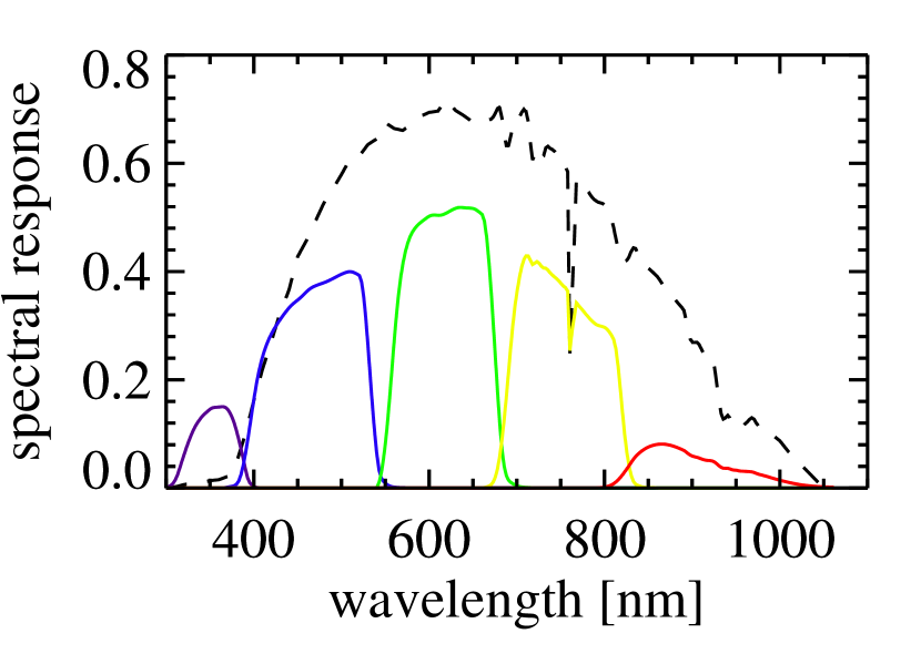
The two telescopes of the LINEAR project are each equipped with a CCD camera developed at MITLL using CCDs developed and manufactured by MITLL for the US Air Force GEODSS system (Burke et al., 1998). These CCID-16 sensors are 5 megapixel (2560x1960), back-illuminated, frame-transfer CCDs with fast readout, low dark current, and low read noise. The CCID-16 sensors have 8 readout regions (hereafter referred to as cells) and have high quantum efficiency over a broad part of the visible and near-infrared spectrum (with overall solar-weighted quantum efficiency of 65% and peak efficiency of 96% at 620 nm, see Figure 1). The cameras have no spectral filters. The combination of the CCID-16 camera and the 1-m GEODSS telescope produces an instantaneous field-of-view of by ( deg2), with pixels. In Section 3, the combination of CCID-16 sensors and L1 and L2 telescopes will be referred to as the L1 and L2 setups.
For a few months in 2003 (approximately August to November) the camera on the L2 telescope was replaced with a very similar camera containing a smaller format sensor called the CCID-10. This smaller sensor is identical to the CCID-16s in terms of manufacture and processing, readout electronics and settings, spectral quantum efficiency and pixel size. The only difference between the smaller format camera and the larger format camera is the number of pixels, 1024x1024 for the small camera, and the number of readout regions (4 cells). During the four months in 2003 that L2 was operating with the CCID-10 camera, the field-of-view was about by ( deg2). In Section 3, the combination of CCID-10 sensor and L2 telescope will be referred to as the small setup.
2.2 Observing Conditions and Cadence
The telescope site has reasonably dark skies, approaching mag arcsec-2 on the best nights. However, the LINEAR program operates on nights with suboptimal conditions including haze, bright moonlight (to within 3 days of the full moon), scattered clouds, and airglow. LINEAR images are frequently taken under skies as bright as mag arcsec-2. The point spread function includes unknown contributions from atmospheric seeing and various system contributions (e.g., defocus and dome airflow) and is typically around FWHM, resulting in slightly undersampled images.
The image integration time is allowed to vary over the seasons so that a roughly constant number of search fields fills the available dark time. During the earlier days of the LINEAR program (roughly 1998 to 2006), the integration time was 10-12 seconds on long winter nights and 3-5 seconds on short summer nights. In recent years (roughly 2007 to 2009), the integration time was increased to 15-18 seconds in the winter and 8-13 seconds in the summer. Under these observing conditions, the magnitude for which the magnitude error is mag (the detection limit) is about 18 mag on average.
2.3 Photometry and Astrometry using SExtractor
The LINEAR project has been archiving all of its image data since December 2002 through the present. The data used for this work encompass all imagery collected from December 2002 through March 2008. After selecting the LINEAR imagery data that overlaps the main SDSS survey region (i.e. galactic latitudes greater than ) and SDSS stripe 82 region (, , deg2)), the data comprises about 1.8 million images. The bias and flat-field corrections were applied to these images following standard methodology.
The extraction of sources from LINEAR images and the creation of source catalogs were done using the SExtractor software (Bertin & Arnouts 1996; see the SExtractor users manual111Available at https://www.astromatic.net/pubsvn/software/sextractor/trunk/doc/sextractor.pdf for more details on the source detection and measurement process). The preliminary astrometry for extracted sources was obtained by converting centroid pixel coordinates into equatorial J2000.0 right ascension (R.A.) and declination (Dec) by application of the gnomonic projection and a-priori telescope pointing information. This projection does not correct for telescope pointing errors on the order of several pixels, telescope optical distortion on the order of a few pixels near the corners of the image, or differential refraction on the order of a few pixels at typical airmasses. When compared to the USNO-B catalog (Monet et al., 2003) astrometry, the average uncertainty in the preliminary astrometry is about in R.A. and Dec coordinates. Therefore, the astrometry reported by SExtractor must be recalibrated before matching extracted LINEAR sources against other catalogs. The recalibration of preliminary astrometry is described in the next section.
The preliminary fixed-aperture photometry for each source is computed by summing the pixels within a 5 pixel () radius circular aperture and subtracting the background estimate for each pixel computed in the background estimate step. The uncertainty on the computed flux is computed assuming Poisson statistics in detected electrons with a gain conversion factor of . The pixels with counts above 17000 were not used as the CCDs begin to experience non-linear response above this level (corresponding to 42000 electrons), and they saturate at full-well capacity of 75,000 electrons.
3 Recalibration of LINEAR astrometry and photometry
In this Section, we describe the astrometric and photometric recalibration of LINEAR data and quantify the quality of recalibrated data. The recalibration and data quality assessment are done on a field-by-field basis, where a field is defined as part of a LINEAR image observed by a single CCD cell (there are 4 cells in the small setup and 8 cells in the L1 and L2 setups). The only exception to this is the astrometric recalibration, which is done on a image-by-image basis. However, the quality of astrometric recalibration is still assessed on a field-by-field basis.
3.1 Astrometric recalibration
We recalibrate the preliminary astrometry using the Astrometry.net software (Lang et al., 2010). The Astrometry.net uses the and (hereafter, pixel) positions of sources extracted by SExtractor and looks for “skymarks” (sets of four stars) that correspond to pre-computed “skymarks” found in the “clean” USNO-B catalog (Barron et al., 2008). Once a skymark is found the code obtains an initial astrometric solution (a transformation from the pixel coordinates into the J2000.0 Equatorial system) in the form of a third-degree polynomial in and coordinates. Using this initial astrometric solution the code looks for additional reference USNO-B stars in the image, and when it finds them it further refines the initial astrometric solution.
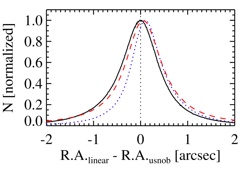
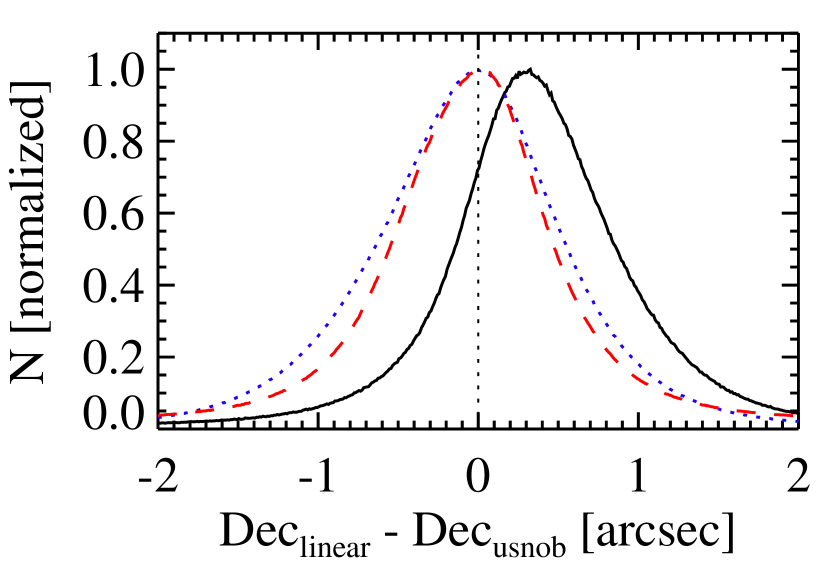
The quality of recalibrated LINEAR astrometry is estimated by comparing the LINEAR positions with reference USNO-B positions (Figure 3). We find that the recalibrated LINEAR single-epoch coordinates have an rms scatter of and are offset with respect to the USNO-B coordinates. These systematic offsets are independent of pixel positions or the position of the image on the sky, and are subtracted from recalibrated LINEAR coordinates. Using a subset of data, we have found that the offsets decrease if the Astrometry.net is allowed to search for even more reference USNO-B stars when refining the initial astrometric solution.
To find fields with bad astrometry, we calculate the median and rms scatter of astrometric residuals (difference between LINEAR and USNO-B positions) in R.A. and Dec for each field, and tag fields as bad if the median or rms scatter in either coordinate (R.A. or Dec) is greater than . We find that about 7% of all fields have bad astrometry, with the majority of bad fields () originating from the L2 setup, and remove them from further processing. Visual inspection of images containing bad fields revealed that bad fields lack several pixel columns, which were most probably dropped due to cell readout problems.
In order to recalibrate the LINEAR photometry, we positionally matched the LINEAR dataset to the Sloan Digital Sky Survey Data Release 7 (SDSS DR7; Abazajian et al. 2009) imaging catalog. The SDSS DR7 imaging catalog provides homogeneous and deep () 1-2% accurate photometry in five band-passes (, , , , and ) of more than 11,000 deg2 of the North Galactic Cap, and three stripes in the South Galactic Cap totaling 740 deg2. The SDSS positions are accurate to better than per coordinate (rms) for sources with (Pier et al., 2003), and the morphological information from the images allows reliable star-galaxy separation to (Lupton et al., 2002).
We match LINEAR sources to SDSS DR7 non-saturated, “primary” objects222See http://cas.sdss.org/dr6/en/help/docs/algorithm.asp?key=flags using a radius, and find billion matched pairs (there are 24 million unique SDSS sources included in these pairs). There are billion LINEAR sources without a SDSS match (“orphans”), and they include observations associated with stars saturated in SDSS (, of orphans), image artifacts (e.g., due to charge bleeding and diffraction spikes), moving objects such as asteroids, and other transients.
3.2 Photometric recalibration
We model the recalibrated LINEAR magnitudes as
| (1) |
where measures non-linearity of SExtractor-supplied instrumental magnitudes , is a color-dependent term that accounts for the per-exposure change in the effective central wavelength of the LINEAR bandpass, and is our model for the field-specific magnitude zero-point dependent on the position in the image, defined as
| (2) |
where , , and vary from field to field, and is the “super flat-field” (fixed for each observational setup). Note that the color-independent airmass term (gray extinction) is implicitly included in .
To recalibrate the LINEAR photometry we need a catalog of photometric standard stars in the LINEAR photometric (unfiltered) system. Since such a catalog does not exist, we use the SDSS imaging catalog and utilize SDSS photometry to derive magnitudes in the LINEAR photometric system.
3.2.1 LINEAR Magnitudes Synthesized from SDSS Photometry
We define LINEAR magnitudes synthesized from the SDSS photometry as
| (3) |
where is some function of , and SDSS magnitudes are not corrected for the ISM extinction.
We find iteratively by first adopting in Equation 1, in Equation 2, and in Equation 3. For each field, we determine , and by minimizing
| (4) |
where is the magnitude error supplied by the SExtractor (errors in are assumed to be much smaller than errors in ).
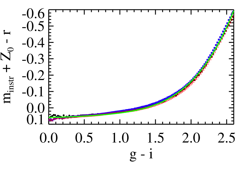
The LINEAR observations of calibration stars must be matched within to isolated333SDSS CHILD flag set to 0, unresolved, SDSS objects brighter than , with . Having for each field, we calculate residuals for all calibration stars, bin the values in bins, and plot the median residuals in Figure 4 for the small, L1, and L2 setup. We plot medians for each setup separately because each setup represents a separate optical, and therefore photometric, system.
Even though the three setups are different, their residuals depend similarly on (rms scatter around the mean is 0.01 mag), as indicated by medians plotted in Figure 4. We therefore fit a fourth-degree polynomial to all medians, and obtain
| (5) |
The transformation from SDSS to LINEAR magnitudes, as defined by Equation 3, is then
| (6) |
This equation effectively turns the SDSS imaging catalog into a catalog of LINEAR photometric standard stars.
3.2.2 Super Flat-fields and Non-linearity of Instrumental Magnitudes
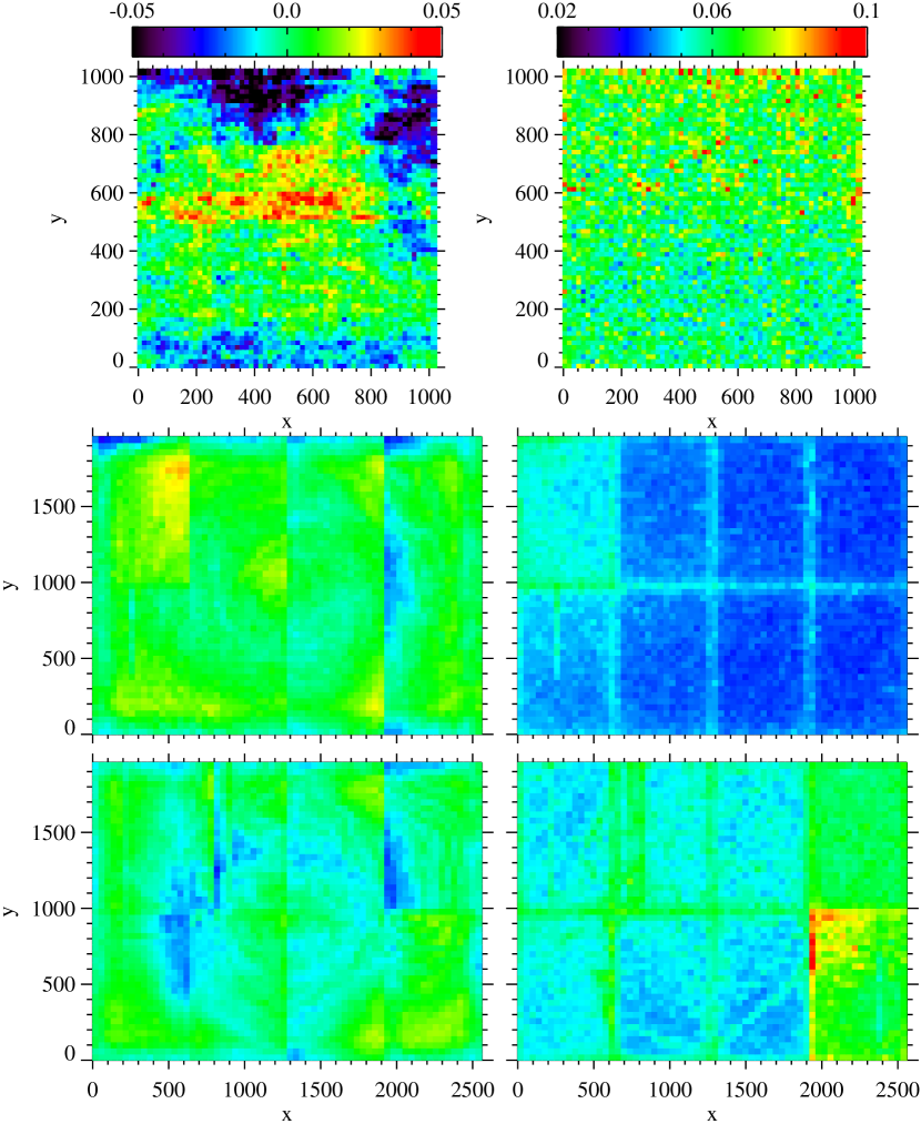
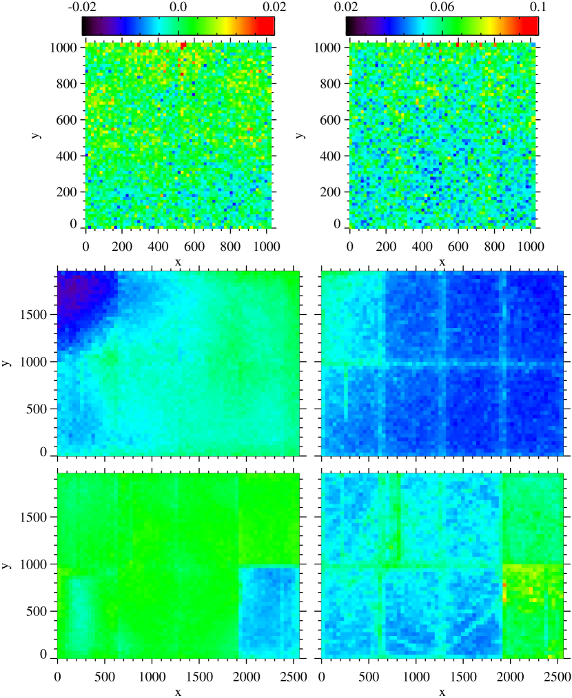
We find super flat-field, , iteratively by first adopting in Equation 1 and in Equation 2. For each field, we determine , , , and by minimizing Equation 4 using calibration stars brighter than . The super flat-field correction, , is then obtained by finding the median of residuals binned in pixels, and is shown as a color-coded map in Figure 5 (left) for each observational setup. Figure 6 (left) shows the residuals after the subtraction of Figure 5 (left) maps. On average, the median residuals are now smaller than 0.005 mag, compared to mag before the correction was made.
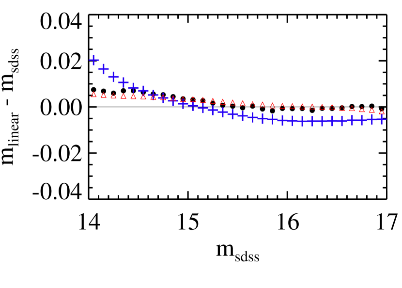
To verify our assumption of (the linearity of instrumental magnitudes), we adopt in Equation 1, and determine , , , and by minimizing Equation 4 using calibration stars brighter than . We bin residuals in bins, and plot the medians as a function of in Figure 7. A strong dependence of residuals on would indicate non-linear () behavior of instrumental magnitudes. With the exception of a small non-linearity ( mag) in the L1 setup for , the residuals do not depend on magnitude indicating that the assumption is valid.
To estimate the magnitude of correction introduced by including the color-dependent term (accounts for the change in LINEAR bandpass due to varying airmass) in Equation 1, we measure the rms scatter of values obtained from all calibration stars and fields. We find the rms scatter to be mag indicating that by correcting for this term the systematic uncertainty in LINEAR photometry is reduced by mag. On the other hand, the inclusion of the term is much more important as it reduces the systematic uncertainty in LINEAR photometry by mag (the rms scatter of values is mag).
Once the color-dependent term, , and the zero-point, , are obtained for a field, the LINEAR photometry for that field is recalibrated using Equation 1. For “orphan” sources (LINEAR sources not associated with SDSS objects) the color-dependent term is set to , as colors are not available for these sources. Therefore, the systematic uncertainty in recalibrated photometry is slightly higher for orphans (by mag).
3.2.3 Checks on Recalibrated Photometry
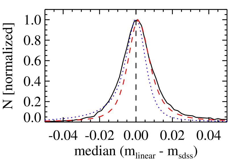
To quantify the quality of recalibration on a field-to-field basis, we calculate residuals for calibration stars, and find their median and rms scatter (determined from the interquartile range) for each field. The median of () residuals per field is then an estimate of the zero-point error. The distribution of these median offsets, shown in Figure 8, is about 0.01 mag wide and demonstrates the overall quality of recalibrated photometry. About 10% of fields are of low-quality (rms scatter in mag), usually due to highly variable cloud coverage. Sources detected in such fields are removed from further consideration.
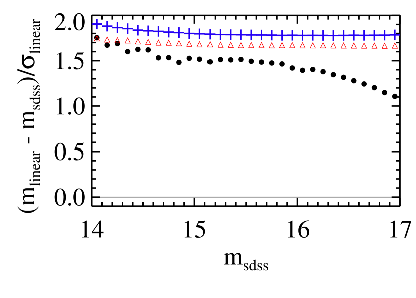
Another useful statistic is the rms scatter of values, , in bins. This rms scatter should be equal to 1 and should not depend on if the SExtractor-supplied magnitude errors () are correct Gaussian errors. As shown in Figure 9, the rms scatter is greater than 1 indicating underestimated errors by up to a factor of .
We correct underestimated magnitude errors by multiplying them by 1.4, 1.85, and 1.65 for the small, L1, and L2 setup, respectively. In case of the small setup, the factor of 1.4 is only the average value as SExtractor-supplied magnitude errors for that setup seem to depend on magnitude. Therefore, the magnitude errors for the small setup may be slightly overestimated or underestimated depending on the brightness of the source. This is not a major issue as only a small fraction of all LINEAR sources () originate from the small setup.
The reason for this underestimation of SExtractor-supplied magnitude errors is not clear. Non-inclusion of systematic errors (e.g., due to flat-fielding) in cannot explain this behavior for L1 and L2 setups. If additive systematic errors were the reason for this underestimation, then should decrease with magnitude because is expected to increase with magnitude (see Figure 13). Yet, no such decrease is seen in Figure 9 for L1 and L2 setups.
4 Characterization of the Recalibrated LINEAR Dataset
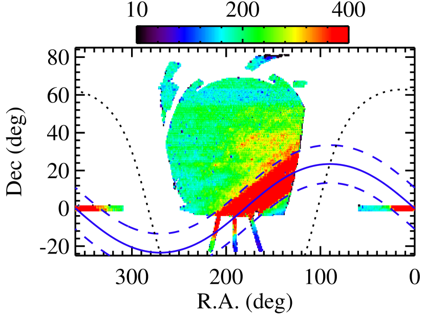
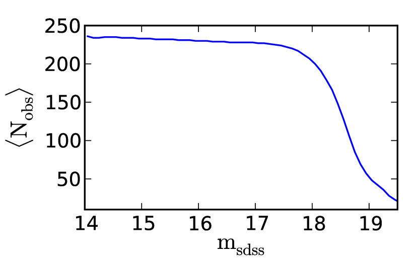
There are about 5 billion sources in the recalibrated LINEAR dataset. These sources were grouped into clusters using an implementation of the OPTICS algorithm (Ankerst et al., 1999) and a clustering radius of . There are about 25 million clusters with more than 15 observations. SDSS provides morphological classification for 24 million clusters (7 million are resolved and 17 million are unresolved by SDSS), and for 1 million of these clusters there is no SDSS classification (they are slightly outside the SDSS footprint). Clusters with 15 or more sources are hereafter labeled as LINEAR objects or time-series. The median number of epochs (observations) per object as a function position and magnitude is shown in Figures 10 and 11. The average number of epochs for objects brighter than 18 mag within of the ecliptic plane is , and elsewhere.
Clusters with less than 15 sources are not tagged as objects. We have statistically analyzed properties of 385 million sources ( of all LINEAR sources) assigned to such clusters and have found that most of them are very faint (), have very uncertain magnitudes ( mag), and have high ellipticity (suggestive of cosmic rays and image artifacts). Such clusters and their observations are not included in our database. This also means that the LINEAR database does not include observations of fast moving objects (i.e. objects moving faster than day-1).
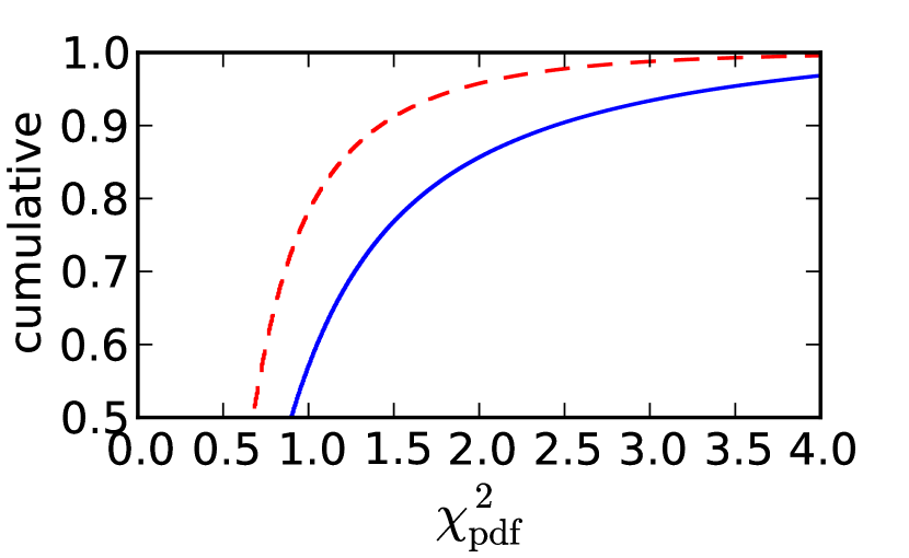
In order to enable discovery of variable objects and to further characterize the LINEAR dataset, we have computed various low-order statistics for time-series, such as the median recalibrated magnitude (), rms scatter (), per degree of freedom (), skewness (), and kurtosis (). The cumulative distributions of for LINEAR objects with more than 30 observations are shown in Figure 12.
The median of the distribution for bright LINEAR objects () is about 1, indicating that, on average, the uncertainties in LINEAR magnitudes are well determined. For fainter LINEAR objects (), the median of the distribution is slightly lower () indicating slightly overestimated photometric errors.
The high-end tail () of the cumulative distribution suggests that of bright LINEAR objects exhibit deviations from the mean that are inconsistent with the Gaussian distribution of errors. These objects could be variable or could have unreliable (non-Gaussian) errors. While it is not impossible that some fraction of LINEAR objects are variable ( of sources brighter than are variable, see Sesar et al. 2006 and references therein), a fraction of seems unlikely. A more likely explanation is spurious variability induced by non-Gaussian errors, caused by blending of sources and unaccounted instrumental defects (e.g., bad pixels).
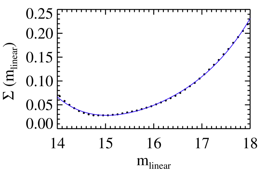
To estimate the dependence of the median photometric error () on magnitude, we follow Sesar et al. (2007) and calculate median values in bins. The dependence of median on , shown in Figure 13, can be modeled as a fourth-degree polynomial
| (7) |
where . The smallest photometric errors are at ( mag) and are limited by systematic errors in calibration. The increase in photometric error at brighter magnitudes is probably due to saturation issues in LINEAR. The photometric error starts to increase rapidly towards fainter magnitudes due to photon noise, and reaches mag at (the adopted faint limit).
In addition to statistics calculated on light curves, we also calculated time-averaged positions (median and mean right ascension and declination). To estimate the reliability of time-averaged LINEAR positions, we compared them to SDSS positions in deg2 pixels on the sky and calculated the median difference in positions for each pixel. We find that, on average, the time-averaged LINEAR positions are within of SDSS positions, with no systematic trends across the sky. The largest median difference (for a deg2 pixel) is . While this precision is sufficient for most applications, we still recommend that SDSS positions are used whenever possible to avoid patches where time-averaged LINEAR positions may be less reliable.
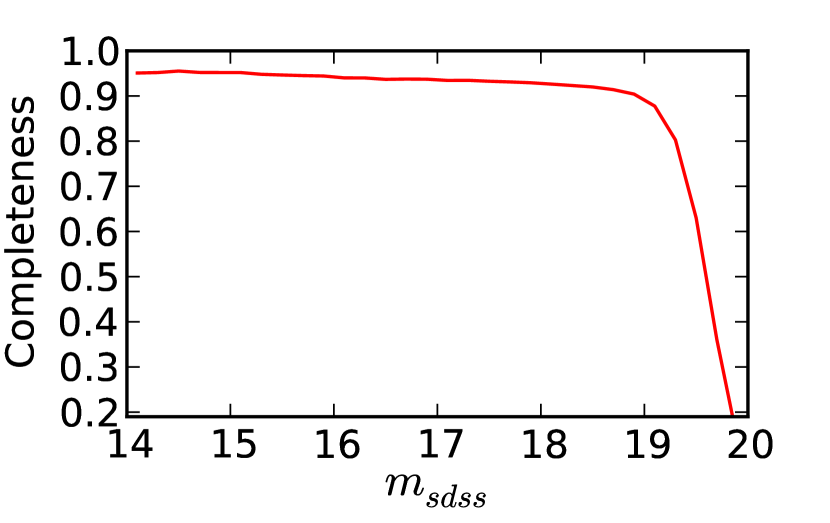
Since SDSS is about 4 mag deeper than LINEAR, it can be used to estimate the completeness of the LINEAR object catalog (i.e., LINEAR object catalog is a subset of the SDSS object catalog). To estimate the completeness of the LINEAR object catalog, in Figure 14 we plot the fraction of SDSS objects matched to LINEAR objects as a function of (LINEAR magnitude synthesized from SDSS photometry, see Equation 6). For this purpose we use SDSS and LINEAR objects with (color range where Equation 6 is valid), , and . As shown in Figure 14, the LINEAR object catalog is more than 90% complete for . This estimate may be a bit misleading as the criterion for object creation is having at least 15 detections. Even faint objects () are likely to be detected at least 15 times out of an average of 200 observations (see Figure 11), if the observing conditions are better than average (e.g, due to better seeing and darker skies).
5 Preliminary Analysis of Variable Objects Selected from the LINEAR Dataset
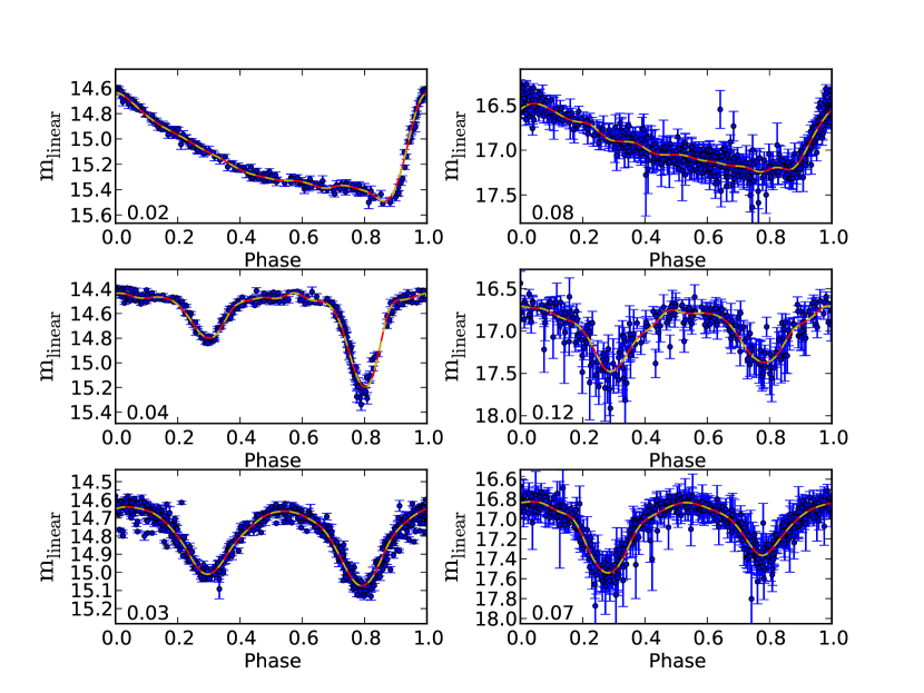
We have examined a small subset of objects with (5,000) and identified a subset of periodically variable stars. We confirmed expectation from the preceding Section that only a few percent of the subsample are convincing cases of periodic variability. As an illustration of the quality of LINEAR light curves at the bright () and faint end (), we show their period-folded light curves in Figure 15. The main strength of the LINEAR survey is easily discernible in these plots: even at the faint end, the light curve features are well defined thanks to dense LINEAR sampling.
To exploit the full potential of the LINEAR photometric database, an automated selection and classification of variable objects is desirable. This desideratum is not easy to accomplish because the fraction of spurious objects with is an order of magnitude larger than the fraction of truly variable objects. In order to enable the deployment of automated selection and classification methods, we have undertaken an extensive program of visual light curve classification. Details of this program are described in a companion paper (Palaversa, L. et al. 2011, in preparation, hereafter Paper II) and here we only provide a brief description of the variable candidate selection and their distribution in various color-color diagrams.
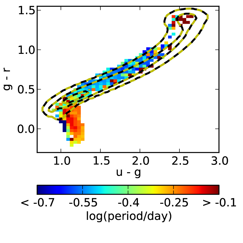
In the first step, we define a flux-limited sample of objects with and select about 200,000 light curves with and mag ( is the rms scatter in the light curve). We limit classification to objects exhibiting periodic variability and use phased light curves for visual inspection. The periods are determined using the Supersmoother algorithm (Reimann, 1994). In total, about 7,000 LINEAR objects (3.5% out of 200,000) were visually confirmed as periodic variables, with about two thirds classified as RR Lyrae type stars and eclipsing binary stars of all types. The remaining 1/3 include SX Phoenicis and Delta Scuti stars, long-period variables, as well as possible RR Lyrae type and eclipsing binary stars with less certain classification. The distributions of classified objects in the SDSS vs. color-color diagram is shown in Figure 16.
The differences between the distributions of all sources and those of the confirmed variable subsample demonstrate that the latter are robustly classified (i.e., the classification is not random). The most obvious difference is a much higher fraction of RR Lyrae stars in the classified sample (, ). The eclipsing binary systems of all types dominate the visually classified sample in the main stellar locus region. There seems to be a hint for the median period of eclipsing binaries becoming longer for bluer stars. The distribution of eclipsing stars is offset from the distribution of all stars in the direction perpendicular to the stellar locus (offset to upper left). There is also a lack of variable (eclipsing) systems of the late K and early M spectral type. These results are discussed in more detail in Paper II.
6 Summary
In this work we have described astrometric and photometric recalibration of data obtained by the asteroid survey LINEAR. The public access to the recalibrated LINEAR dataset will be provided through the SkyDOT Web site (http://skydot.lanl.gov). A description of various cataloged parameters that are available in this database is given in Appendix B.
The preliminary astrometry produced by the survey has been recalibrated using the Astrometry.net software and USNO-B catalog as the reference astrometric catalog. The precision (rms scatter) of single-epoch recalibrated LINEAR coordinates is with respect to the reference (USNO-B) astrometric catalog. The precision of time-averaged LINEAR coordinates is with respect to SDSS positions.
In order to recalibrate the LINEAR photometry, we positionally matched the LINEAR dataset to the SDSS DR7 imaging catalog and used SDSS as a catalog of photometric standard stars. LINEAR instrumental magnitudes were corrected for changes in the LINEAR bandpass (due to varying airmass) and for zero-point variations across the CCD (due to imperfect flat-fielding). These corrected LINEAR magnitudes were then offset on a per-LINEAR field basis to match the SDSS magnitude zero-point system. In general, the recalibrated LINEAR magnitudes () behave linearly, with the exception of a small non-linearity ( mag) in the L1 setup at magnitudes brighter than 15 mag.
We find the average uncertainty in recalibrated LINEAR magnitudes to be mag at the bright end (, the systematic uncertainty) and mag at the faint end (, the adopted faint limit for the survey). The SExtractor-supplied magnitude errors were found to be underestimated by , independent of magnitude, and were subsequently corrected for this behavior using multiplicative factors.
There are about 5 billion photometric measurements in the recalibrated LINEAR dataset. The sources detected in each observation were grouped into clusters (time-series or objects) using a clustering radius of . There are about 25 million clusters with at least 15 observations (7 million resolved and 17 million unresolved by SDSS, the rest without morphological classification). The median number of epochs (observations) per object brighter than 18 mag and within of the ecliptic plane is , and elsewhere. The completeness of the LINEAR object catalog (relative to the SDSS imaging catalog) was estimated to be better than 90% for sources brighter than 19 mag.
LINEAR dataset represents a major new resource for studying the variability of faint optical sources. With an average of 200 observations per object, LINEAR data provide time domain information for the brightest 4 magnitudes of the SDSS survey. At the same time, LINEAR significantly extends the deepest similar wide-area variability survey, the Northern Sky Variability Survey, by 3 mag.
In order to help automated discovery of variable objects, we have computed various low-order statistics for time-series (median recalibrated magnitude, rms scatter, per degree of freedom, skewness, and kurtosis). The distribution for bright LINEAR objects (brighter than 17 mag) is centered at (indicating that, on average, the uncertainties in LINEAR magnitudes are well determined), and has a long high-end () tail. About 5% of LINEAR objects have ; in a sample with Gaussian errors, less than 0.01% of objects are expected to have . This high-end tail is populated by truly variable objects, but is most likely dominated by spuriously variable objects with unreliable (non-Gaussian) errors (caused by, for example, unaccounted instrumental defects such as bad pixels or by blended sources).
Since the fraction of spurious variable objects is at least a few times greater than the fraction of truly variable objects, we have undertaken an extensive program of visual light curve classification in order to enable future deployment of automated methods. Details of this program are described in a companion paper (Palaversa, L. et al. 2010, in preparation).
Appendix A LINEAR Observing Strategy
To search for asteroids, the LINEAR program attempts to cover the entire portion of sky available from the site each lunar month (lunation), with repeat searches within 10 to 15 degrees of the ecliptic plane. The program schedules searches on both telescopes an average of 25 nights per lunation, taking off 4-5 nights around the full moon. After accounting for weather and equipment problems, about 20 observing nights are achieved per lunation with each telescope. To minimize stray light, the survey fields are kept about away from the moon during the week before and after the full moon.
To efficiently cover the available sky at minimal airmass, each telescope is assigned a strip of sky that is aligned with either the ecliptic or the equator and is typical 3-4 fields of view () wide in declination or ecliptic latitude, and 150 fields of view () long in right ascension or ecliptic longitude. The search box is divided into 5-7 regions each containing about 100 fields. The regions are searched starting with the westernmost region at the beginning of astronomical twilight in the evening, and ending with the easternmost region at the end of astronomical twilight in the morning. All of the fields in a single region are imaged in sequence, and then the sequence is repeated in that region 4 more times. The 5 images of a given field are combined into a “frameset” which forms the input to a moving target detection algorithm that distinguishes asteroids from stars and noise based on their motion. This process of cycling through the fields in a region 5 times produces a temporal separation of 15 to 20 minutes between successive images of the same patch of sky.
On subsequent nights, the entire search area for each telescope is generally stepped north or south by the height of the region in order to cover the entire sky, though gaps are occasionally unavoidable due to missed nights. Over the course of one lunation the entire available sky is generally searched once, and areas within about of the ecliptic are searched two or three times. Because the monthly search regions are quite wide in right ascension, there is significant overlap in coverage area on adjacent lunar months. Therefore, a given patch of sky can be observed up to 8 months in a row before it passes into the daytime portion of the sky for 4 months. After a full year the search covers the entire sky north of declination except for a small circle north of declination where the telescope has poor settling ability. LINEAR’s pattern of sky coverage produces repeat photometry data for stars on several timescales ranging from the 15-20 minute interval between images within a frameset, to a few days between repeat visits during one lunation, to the month-long timescale between lunar months, to the yearly.
Appendix B LINEAR Database Schema
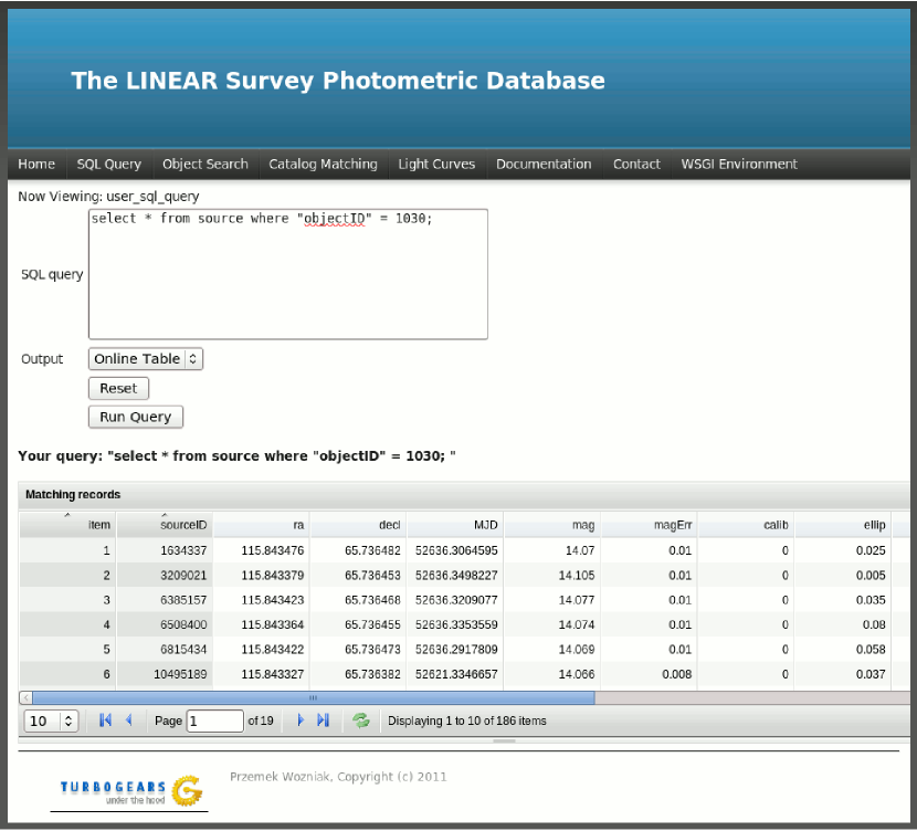
The LINEAR database hosted at SkyDOT contains two tables, “Object” and “Source”. The “Source” table contains photometry and astrometry of individual LINEAR detections (sources), while the “Object” table references time-series obtained by clustering sources within . In addition, the “Object” table contains various low-level statistics calculated on time-series and is cross-matched to external catalogs such as SDSS and 2MASS (Skrutskie et al., 2006). A detailed description of various parameters provided by these tables is given in Tables 1 and 2, and a screenshot showing the SkyDOT interface is shown in Figure 17.
References
- Abazajian et al. (2009) Abazajian, K. et al. 2009, ApJS, 182, 543
- Akerlof et al. (2000) Akerlof, C. et al. 2000, AJ, 119, 1901
- Andersen (1991) Andersen, J. 1991, A&A Rev., 3, 91
- Ankerst et al. (1999) Ankerst, M. et al. 1999, “Proceedings of the 1999 ACM SIGMOD International Conference on Management of Data”, 49
- Barron et al. (2008) Barron, J. T. et al. 2008, AJ, 136, 1490
- Becker et al. (2004) Becker, A. C. et al. 2004, ApJ, 611, 418
- Bertin & Arnouts (1996) Bertin, E. & Arnouts, S. 1996, A&A Supplement, 117, 393
- Burke et al. (1998) Burke, B. et al. 1998, Experimental Astronomy, 8, 31-40
- Covey et al. (2007) Covey, K. R. et al. 2007, AJ, 134, 2398
- Guinan et al. (1998) Guinan, E.F. et al. 1998, ApJ, 509, L21
- Ivezić et al. (2008) Ivezić, Ž. et al. 2008, arXiv:0805.2366
- Kaiser et al. (2002) Kaiser, N. et al. 2002, Proc. SPIE, 4836, 154
- Lang et al. (2010) Lang, D. et al. 2010, AJ, 139, 1782
- Law et al. (2009) Law, N. M. et al. 2009, PASP, 121, 1395
- Lupton et al. (2002) Lupton, R. H. et al. 2002, Proc. SPIE, 4836, 350
- Miceli et al. (2008) Miceli, A. et al. 2008, ApJ, 678, 865
- Monet et al. (2003) Monet, D. G. et al. 2003, AJ, 125, 984
- Munn et al. (2004) Munn, J. A. et al. 2004, AJ, 127, 3034
- Pier et al. (2003) Pier, J. R. et al. 2003, AJ, 125, 1559
- Pojmański (2002) Pojmański, G.2002, Acta Astron., 52, 397
- Prša & Zwitter (2005) Prša, A. & Zwitter, T. 2005, ApJ, 628, 426
- Rau et al. (2009) Rau, A. et al. 2009, PASP, 121, 1334
- Reimann (1994) Reimann, J. D. 1994, Ph.D. thesis, Univ. California, Berkeley
- Sesar et al. (2006) Sesar, B. et al. 2006, AJ, 131, 2801
- Sesar et al. (2007) Sesar, B. et al. 2007, AJ, 134, 2236
- Skrutskie et al. (2006) Skrutskie, M. F. et al. 2006, AJ, 131, 1163
- Stokes et al. (2000) Stokes, G. et al. 2000, Icarus, 148, 21
- Torres, Andersen & Giménez (2010) Torres, G., Andersen, J. & Giménez, A. 2010, A&A Rev., 18, 67
- Woźniak et al. (2004) Woźniak, P. R. et al. 2004, AJ127, 2436
- York et al. (2000) York, D. G. et al. 2000, AJ, 120, 1579
| Field | Description |
|---|---|
| sourceID | A unique number identifying this source |
| ra | Equatorial J2000.0 right ascension |
| decl | Equatorial J2000.0 declination |
| MJD | Modified Julian Date |
| mag | Recalibrated LINEAR magnitude |
| magErr | Uncertainty in the recalibrated LINEAR magnitude |
| calib | 1 if the source was used for calibration, 0 otherwise |
| ellip | “Ellipticity” parameter measured by SExtractor |
| ximg | Position of the source along CCD’s axis |
| yimg | Position of the source along CCD’s axis |
| FWHM | Full-Width-At-Half-Maximum measured by SExtractor |
| flagsa | SExtractor internal flags |
| objectID | A number associating this source with an object in the “Object” table |
| Field | Description |
|---|---|
| objectID | A unique number identifying this object |
| ra | Mean equatorial J2000.0 right ascension |
| decl | Mean equatorial J2000.0 declination |
| ra_std | Rms scatter in right ascension (in units of arcsec) |
| decl_std | Rms scatter in declination (in units of arcsec) |
| ra_median | Median equatorial J2000.0 right ascension |
| decl_median | Median equatorial J2000.0 declination |
| nptsTotal | Number of detections |
| nptsGood | Number of detections with flags0 |
| mag_mean | Mean recalibrated LINEAR magnitude |
| mag_wmean | Weighted recalibrated LINEAR magnitude (by magnitude errors) |
| mag_median | Median recalibrated LINEAR magnitude |
| mag_std | Rms scatter of recalibrated LINEAR magnitudes |
| mag_wstd | Weighted rms scatter of recalibrated LINEAR magnitudes (by magnitude errors) |
| mag_skew | Skewness of recalibrated LINEAR magnitudes |
| mag_kurtosis | Kurtosis of recalibrated LINEAR magnitudes |
| mag_chi2dof | per degree of freedom around the mean magnitude |
| mag_rchi2dofa | Robust per degree of freedom around the mean magnitude |
| theta_sdssb | Distance in arcsec from the SDSS source |
| sdssID | SDSS Data Release 7 objID parameter |
| sdss_ra | SDSS J2000.0 right ascension |
| sdss_dec | SDSS J2000.0 declination |
| objtype | 6 if unresolved in SDSS imaging (i.e., a point source), 3 if resolved |
| rExt | Extinction in the SDSS -band |
| uMod | SDSS -band model magnitude |
| gMod | SDSS -band model magnitude |
| rMod | SDSS -band model magnitude |
| iMod | SDSS -band model magnitude |
| zMod | SDSS -band model magnitude |
| uErr | SDSS -band model magnitude error |
| gErr | SDSS -band model magnitude error |
| rErr | SDSS -band model magnitude error |
| iErr | SDSS -band model magnitude error |
| zErr | SDSS -band model magnitude error |
| ug | SDSS color (corrected for ISM extinction, ) |
| gr | SDSS color (corrected for ISM extinction, ) |
| ri | SDSS color (corrected for ISM extinction, ) |
| iz | SDSS color (corrected for ISM extinction, ) |
| gi | SDSS color (corrected for ISM extinction, ) |
| pmLc | Proper motion in the Galactic latitude direction (in units of mas/yr) |
| pmBc | Proper motion in the Galactic longitude direction (in units of mas/yr) |
| pmErrc | Proper motion error (in units of mas/yr) |
| isolated | 1 if SDSS CHILD flag is set to 0 (isolated0 may indicate a close neighbor) |
| sdss_satur | 1 if SDSS SATURATED flag is set to 1 |
| sdss_flags | SDSS flags encoded as a 64-bit integer number |
| theta_2massd | Distance in arcsec from the 2MASS source |
| J | 2MASS -band magnitude |
| JErr | 2MASS -band magnitude error |
| H | 2MASS -band magnitude |
| HErr | 2MASS -band magnitude error |
| K | 2MASS -band magnitude |
| KErr | 2MASS -band magnitude error |
| jh | 2MASS color (corrected for extinction, ) |
| hk | 2MASS color (corrected for extinction, ) |
| jk | 2MASS color (corrected for extinction, ) |
