Phenomenology of ageing in the Kardar-Parisi-Zhang equation

Abstract

We study ageing during surface growth processes described by the one-dimensional Kardar-Parisi-Zhang equation. Starting from a flat initial state, the systems undergo simple ageing in both correlators and linear responses and its dynamical scaling is characterised by the ageing exponents $a=-1/3$, $b=-2/3$, $\lambda_{C}=\lambda_{R}=1$ and $z=3/2$. The form of the autoresponse scaling function is well described by the recently constructed logarithmic extension of local scale-invariance.

The study of the motion of interfaces continues as a widely fascinating topic of statistical physics. One particularly intensively studied case is non-equilibrium growth processes, which are governed by local rules. Of these, the model equation proposed by Kardar, Parisi and Zhang (KPZ) Kard86 continues to play a paradigmatic role in the investigation of the dynamical scaling of such interfaces, with an astounding range of applications, including Burgers turbulence, directed polymers in a random medium, glasses and vortex lines, domain walls and biophysics, see Bara95 ; McKa95 ; Halp95 ; Krug97 ; Krie10 ; Sasa10b ; Tong94 ; Batc00 for reviews. Remarkably, in $1D$ the height distribution can be shown to converge for large times towards the gaussian Tracy-Widom distribution Sasa10 ; Cala11 . A particularly clean experimental realization of this universality class has been found recently in the growing interfaces of turbulent liquid crystals Take11 .

New insight in the non-equilibrium properties of many-body systems comes from an analysis of the ageing properties, which is realised if the system is rapidly brought out of equilibrium by a change of one of its state variables Cugl02 ; Henk10 . By definition, an ageing system (i) undergoes a slow, non-exponential relaxation towards its stationary state(s), (ii) does not satisfy time-translation-invariance and (iii) shows dynamical scaling. Studies of ageing require the analysis of both correlators $C$ and responses $R$ to be complete and also go beyond the study of dynamics in analysing at least two-time observables. Let $s$ denote the waiting time and $t>s$ the observation time. For simple ageing, one expects in the ageing regime $s\gg\tau_{\rm micro}$ and $t-s\gg\tau_{\rm micro}$, where $\tau_{\rm micro}$ is a microscopic time scale, a single relevant length scale $L(t)\sim t^{1/z}$ such that

$$C(t,s) = \left\langle\phi(t)\phi(s)\right\rangle-\left\langle\phi(t)\right\rangle\left\langle\phi(s)\right\rangle=s^{-b}f_{C}\left(\frac{t}{s}\right)$$ (1)

$$R(t,s) = \left.\frac{\delta\left\langle\phi(t)\right\rangle}{\delta j(s)}\right|_{j=0}=\left\langle\phi(t)\widetilde{\phi}(s)\right\rangle=s^{-1-a}f_{R}\left(\frac{t}{s}\right)$$

where $j$ is the external field conjugate to $\phi$. This defines the ageing exponents $a,b$ and the scaling functions, from whose asymptotic behaviour $f_{C,R}(y)\sim y^{-\lambda_{C,R}/z}$ as $y\to\infty$ one has the autocorrelation and autoresponse exponents $\lambda_{C,R}$ where $z$ is the dynamical exponent. In the context of Janssen-de Dominicis theory, $\widetilde{\phi}(t)$ is the response field conjugate to the order-parameter $\phi(t)$.

For example, simple ageing is found in non-disordered, unfrustrated magnets, quenched from an initial disordered state to a temperature $T\leq T_{c}$ at or below its critical temperature $T_{c}$ (see Henk10 and refs. therein) or else in microscopically irreversible systems with a non-equilibrium stationary state Enss04 ; Rama04 ; Odor06 ; Dura11 . Generically, one finds $\lambda_{C}=\lambda_{R}$, but the values of $a,b$ depend more sensitively on the kind of ageing investigated (for reversible systems on the type of quench and for irreversible ones on the specific type of dynamics).

Here, we shall study what kind of ageing phenomena can arise in the growth of interfaces. A typical system is formulated in terms of a height variable $h=h_{i}(t)=h(t,{\bf{r}}_{i})$, defined over a substrate in $d$ dimensions. A local, microscopic rule indicates how single particles are added to the surface. One of the main quantities studied is the surface roughness

$$w^{2}(t;L)=\frac{1}{L^{d}}\sum_{i=1}^{L^{d}}\left\langle\left(h_{i}(t)-\overline{h}(t)\right)^{2}\right\rangle$$ (2)

on a lattice with $L^{d}$ sites and average height $\overline{h}(t)=L^{-d}\sum_{i}h_{i}(t)$. It obeys Family-Vicsek scaling Fami85

$$w^{2}(t;L)=L^{2\zeta}f\left(tL^{-z}\right),\;f(u)\sim\left\{\begin{array}[]{ll}u^{2\beta}&\mbox{\rm;\ if $u\ll 1$}\\ \mbox{\rm cste.}&\mbox{\rm;\ if $u\gg 1$}\end{array}\right.$$ (3)

where $\beta$ is the growth exponent and $\zeta=\beta z$ is the roughness exponent. For an infinite system, the width grows for large times as $w^{2}(t;\infty)\sim t^{2\beta}$.

The generic universality class for growth phenomena is given by the KPZ equation Kard86

$$\frac{\partial h}{\partial t}=\nu\frac{\partial^{2}h}{\partial{\bf{r}}^{2}}+\frac{\mu}{2}\left(\frac{\partial h}{\partial{\bf{r}}}\right)^{2}+\eta$$ (4)

where $\eta(t,{\bf{r}})$ is a white noise with zero mean and variance $\langle\eta(t,{\bf{r}})\eta(t^{\prime},{\bf{r}}^{\prime})\rangle=2\nu T\delta(t-t^{\prime})\delta({\bf{r}}-{\bf{r}}^{\prime})$ and $\mu,\nu,T$ are material-dependent constants. For comparison, we introduce two more universality classes of surface growth: elimination of the non-linear term in (4) by setting $\mu=0$ gives the Edwards-Wilkinson (EW) universality class Edwa82 . The Mullins-Herrings (MH) universality class is given by $\partial_{t}h=-\nu\partial_{r}^{4}h+\eta$ Wolf90 . For both EW and MH classes, the ageing scaling forms (1) for $C$ and $R$ have been explicitly confirmed Roet06 . Values of some growth and ageing exponents in $1D$ are listed in table 1. For the $1D$ KPZ class, the exponents $z,\beta$ are exactly known Kard86 , whereas the relation $b=-2\zeta/z=-2\beta$ follows from dynamical scaling Kall99 ; Daqu11 . Also, evidence for a growing length $L(t)\sim t^{1/z}$ Bust07 ; Chou10 and estimates of $\lambda_{C}$ Kall99 ; Daqu11 have been reported comment1 . However, no systematic test of the ageing scaling has been reported for the space-time correlation function, and no information exists at all for the response function $R$. These will be provided now.

model	$z$	$a$	$b$	$\lambda_{R}=\lambda_{C}$	$\beta$	$\zeta$
KPZ	$3/2$	$-1/3$	$-2/3$	$1$	$1/3$	$1/2$
EW	$2$	$-1/2$	$-1/2$	$1$	$1/4$	$1/2$
MH	$4$	$-3/4$	$-3/4$	$1$	$3/8$	$3/2$

Table 1: Some dynamical, ageing and growth exponents of several universality classes in $d=1$ dimension.

Our numerical simulations in the $1D$ KPZ class either use the discretised KPZ equation (4) in the strong coupling limit Newm97 (we checked that our results do not depend on the chosen discretisation scheme) or else the Kim-Kosterlitz (KK) model Kim89 . This model uses a height variable $h_{i}(t)\in\mathbb{Z}$ attached to the sites of a chain with $L$ sites and subject to the constraints $|h_{i}(t)-h_{i\pm 1}(t)|=0,1$, at all sites $i$. From a flat initial condition, that is $h_{i}(0)=0$, the dynamics of the model is as follows: at each time step, select randomly a site $i$ and deposit a particle with probability $p$ or else eliminate a particle with probability $1-p$. $L$ such deposition attempts make up a Monte Carlo step. It is well-known that this model is in the KPZ universality class. The choice of the value of $p$ is a practical matter. In order to avoid meta-stable states, we have chosen $p=0.98$. In simulations, we have taken $L=2^{17}$ and all the data have been averaged over $10^{4}$ samples. For the discretised KPZ equation we considered systems of size $L=10^{4}$ and averaged over typically $10^{5}$ samples.

In studying the ageing behaviour, we shall consider the two-time spatio-temporal correlator

$$C(t,s;{\bf{r}}) = \left\langle\left(h(t,{\bf{r}}+{\bf{r}}_{0})-{\left\langle\overline{h}(t)\right\rangle}\right)\left(h(s,{\bf{r}}_{0})-{\left\langle\overline{h}(s)\right\rangle}\right)\right\rangle$$ (5)

$$= \left\langle h(t,{\bf{r}}+{\bf{r}}_{0})h(s,{\bf{r}}_{0})\right\rangle-{\left\langle\overline{h}(t)\right\rangle\left\langle\overline{h}(s)\right\rangle}$$

$$= s^{-b}F_{C}\left(\frac{t}{s},\frac{|{\bf{r}}|^{z}}{s}\right)$$

along with the extended Family-Vicsek scaling in the $L\to\infty$ limit and where the definition of the exponents is analogous to the usual one for simple ageing. The autocorrelation exponent can be found from $f_{C}(y)=F_{C}(y,0)\sim y^{-\lambda_{C}/z}$ as $y\to\infty$. We also have $b=-2\beta$, since the width $w^{2}(t;\infty)=C(t,t;{\bf{0}})=t^{-b}F_{C}(1,0)$. This is justified since the initial conditions in the $1D$ KPZ do not generate new, independent renormalisations Krec97 .

 

Figure 1: Scaling of the two-time autocorrelator $C(t,s)$ from the KK model and several values of $s$, and the discretised KPZ equation, with $s=400$, rescaled by a factor $2.79$.

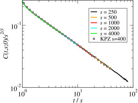
In figure 1, we show data for the autocorrelator $C(t,s)=C(t,s;{\bf{0}})$ obtained from the KK model. A clear data collapse is seen and for large values of the scaling variable $y=t/s$, an effective power-law behaviour with an exponent $\lambda_{C}/z\approx\frac{2}{3}$ is found. The data are fully compatible with a numerical solution of the KPZ equation and directly test simple ageing (1) in the $1D$ KPZ class. All this, completely analogous to the EW and MH classes, confirms and strengthens earlier conclusions Kall99 ; Bust07 ; Chou10 ; Daqu11 ; Krec97 .

In order to define a response, we appeal to the procedures used in irreversible systems Enss04 ; Odor06 ; Dura11 ; Igua09 where the external field is related to a local change of rates. In the KK model, we consider a space-dependent deposition rate $p_{i}=p_{0}+a_{i}\varepsilon/2$ with $a_{i}=\pm 1$ and $\varepsilon=0.005$ a small parameter. Then consider, with the same stochastic noise $\eta$, two realisations: system A evolves, up to the waiting time $s$, with the site-dependent deposition rate $p_{i}$ and afterwards, with the uniform deposition rate $p_{0}$. System B evolves always with the uniform deposition rate $p_{i}=p_{0}$. Of course, the evaporation rate $q_{i}=1-p_{i}$. Then, the time-integrated response function is

$$\chi(t,s;{\bf{r}})=\int_{0}^{s}\!\!{\rm d}u\>R(t,u;{\bf{r}})$$

$$= \frac{1}{L}\sum_{i=1}^{L}\left\langle\frac{h_{i+r}^{(A)}(t;s)-h_{i+r}^{(B)}(t)}{\varepsilon a_{i}}\right\rangle=s^{-a}F_{\chi}\left(\frac{t}{s},\frac{|{\bf{r}}|^{z}}{s}\right)$$

together with the expected scaling. The time-integrated autoresponse $\chi(t,s)=\chi(t,s;{\bf{0}})$ plays the same role as the thermoremanent integrated response of magnetic systems Henk10 . The autoresponse exponent is read off from $f_{\chi}(y)=F_{\chi}(y,0)\sim y^{-\lambda_{R}/z}$ for $y\to\infty$. For the discretised KPZ equation we realize the perturbation by adding a spatially random force, of strength $\pm f_{0}=\pm 0.3$, up to the waiting time $s$.

 

Figure 2: Scaling of the two-time integrated autoresponse $\chi(t,s)$ from the KK model for several values of $s$, and from the KPZ equation with $s=400$, rescaled by a factor $7.25$.

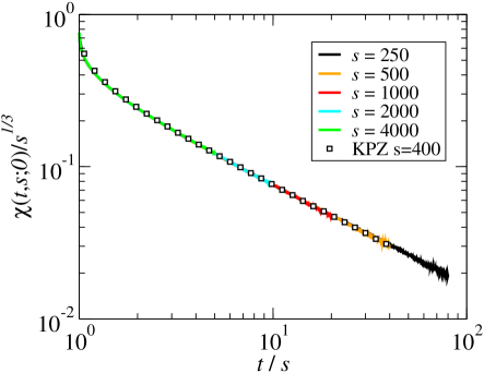
In figure 2, data for the integrated autoresponse $\chi(t,s)$ coming from the KK model are shown. An excellent collapse is found for $a=-\frac{1}{3}$. The effective power law, for $y=t/s$ large, reproduces well the expected $\lambda_{R}/z\approx\frac{2}{3}$. Indeed, from the exact fluctuation-dissipation theorem $TR(t,s;r)=-\partial_{r}^{2}C(t,s;r)$, valid in the $1D$ KPZ universality class (because of time-reversal-invariance) Deke75 ; Lvov93 ; Frey96 ; Cane10 , we obtain the predictions $1+a=b+2/z$ and $\lambda_{C}=\lambda_{R}$, in agreement with our data. The data are essentially identical to those obtained from the KPZ equation, in agreement with universality. For the first time, the ageing form (1) of the linear response is confirmed in a non-linear growth model. In contrast with the EW and MH classes, $a$ and $b$ are different, a feature commonly seen in irreversible systems Henk07 ; Henk10 .

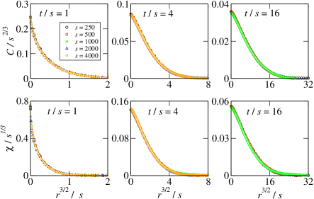
Next, in figure 3, we illustrate the space-dependent scaling of both the correlator and the integrated response. For several values of the scaling variable $y=t/s$, the dependence on the second argument in the scaling forms (5,Phenomenology of ageing in the Kardar-Parisi-Zhang equation) is illustrated. An excellent data collapse is found, which further confirms the conclusions already drawn from the autocorrelator and the autoresponse and also confirms the exactly known dynamical exponent $z=\frac{3}{2}$ in the $1D$ KPZ universality class. The shape of the scaling functions changes notably when $y$ is varied.

 

Figure 3: Space-dependent scaling of the two-time correlator $C(t,s)$ (upper row) and the integrated response $\chi(t,s)$ (lower row), for several values of $s$ and the scaling variable $y=t/s$.

We now turn to an analysis of the form of the autoresponse scaling function $f_{\chi}(y)$. For ageing simple magnets (i.e. non-disordered and unfrustrated), it has been proposed to generalise dynamical scaling to a larger set of local scale-transformations Henk94 , which includes the transformation $t\mapsto t/(1+\gamma t)$. This hypothesis of local scale-invariance (LSI) indeed reproduces precisely the universal shapes of responses and correlators in a large variety of models, as reviewed in detail in Henk10 . Analogous evidence exists in some irreversible models Enss04 ; Odor06 ; Henk07 ; Henk10 . Similarly, the responses and correlators in the EW and MH classes, with the the local height variable $h(t,{\bf{r}})-\overline{h}(t)$ acting as a quasi-primary scaling operator, are described by LSI Roet06 ; Henk07b . Is LSI also realised in the $1D$ KPZ class, with the local height as a quasi-primary operator ?

We concentrate on the autoresponse function and shall restrict attention to the transformations in time. The transformation $\delta\phi=\varepsilon X_{n}\phi$ of the quasi-primary operators under local scale-transformations is given by the infinitesimal generators $X_{n}$, which read Henk06

$$X_{n}=-t^{n+1}\partial_{t}-(n+1)\frac{x}{z}t^{n}-n\frac{2\xi}{z}t^{n}\;\;,\;\;n\geq 0$$ (7)

and satisfy the commutator $[X_{n},X_{m}]=(n-m)X_{n+m}$. We merely look at the finite-dimensional sub-algebra spanned by the dilatations $X_{0}$ and the special transformations $X_{1}$. Since time-translations (generated by $X_{-1}$) are absent, we have two distinct scaling dimensions $x$ and $\xi$, which together give the shape of the autoresponse function, see below. Now, consider a possible extension to so-called logarithmic form, where a primary operator $\phi$ is replaced by a doublet $\left(\begin{array}[]{c}\phi\\ \psi\end{array}\right)$. In analogy with logarithmic conformal invariance Gura93 ; comment2 , this extension is formally carried out by replacing the scaling dimensions $x,\xi$ by matrices (restricted to the $2\times 2$ case) Henk10b

$$x\mapsto\left(\mbox{${\begin{array}[]{cc}x&x^{\prime}\\ 0&x\end{array}}$}\right)\;\;,\;\;\xi\mapsto\left(\mbox{${\begin{array}[]{cc}\xi&\xi^{\prime}\\ \xi^{\prime\prime}&\xi\end{array}}$}\right)$$ (8)

where the first scaling dimension is immediately taken in a Jordan form. Consistency with the commutators then leads to $\xi^{\prime\prime}=0$ Henk10b . Recalling (1), consider the following quasi-primary two-point functions, with $y=t/s$

$$\left\langle\phi(t)\widetilde{\phi}(s)\right\rangle = s^{-(x+\widetilde{x})/z}\>{\cal F}(y)f_{0}$$

$$\left\langle\phi(t)\widetilde{\psi}(s)\right\rangle = s^{-(x+\widetilde{x})/z}\>{\cal F}(y)\Bigl{(}g_{12}(y)+\gamma_{12}\ln s\Bigr{)}$$

$$\left\langle\psi(t)\widetilde{\phi}(s)\right\rangle = s^{-(x+\widetilde{x})/z}\>{\cal F}(y)\Bigl{(}g_{21}(y)+\gamma_{21}\ln s\Bigr{)}$$

$$\left\langle\psi(t)\widetilde{\psi}(s)\right\rangle = s^{-(x+\widetilde{x})/z}\>{\cal F}(y)\sum_{j=0}^{2}h_{j}(y)\ln^{j}s$$ (9)

where ${\cal F}(y)=y^{(2\widetilde{\xi}+\widetilde{x}-x)/z}(y-1)^{-(x+\widetilde{x}+2\xi+2\widetilde{\xi})/z}$ and explicitly known scaling functions Henk10b . In contrast to logarithmic conformal invariance, logarithmic corrections to scaling are absent if $x^{\prime}=\widetilde{x}^{\prime}=0$ and there are no logarithmic factors for $y\to\infty$ if furthermore $\xi^{\prime}=0$. If we take $R(t,s)=\left\langle\psi(t)\widetilde{\psi}(s)\right\rangle=s^{-1-a}f_{R}(t/s)$, we find

$$f_{R}(y)=y^{-\lambda_{R}/z}\left(1-y^{-1}\right)^{-1-a^{\prime}}$$ (10)

$$\times \left[h_{0}-g_{0}\ln\left(1-y^{-1}\right)-\frac{1}{2}f_{0}\ln^{2}\left(1-y^{-1}\right)\right]$$

with the exponents $1+a=(x+\widetilde{x})/z$, $a^{\prime}-a=\frac{2}{z}\left(\xi+\widetilde{\xi}\,\right)$, $\lambda_{R}/z=x+\xi$ and the normalisation constants $h_{0},g_{0},f_{0}$.

The integrated autoresponse $\chi(t,s)=s^{-a}f_{\chi}(t/s)$ is found from (10) by using the specific value $\lambda_{R}/z-a=1$ which holds true for the $1D$ KPZ. We find

$$f_{\chi}(y)=y^{+1/3}\left\{A_{0}\left[1-\left(1-y^{-1}\right)^{-a^{\prime}}\right]\right.$$

$$+ \left.\left(1-y^{-1}\right)^{-a^{\prime}}\left[A_{1}\ln\left(1-y^{-1}\right)+A_{2}\ln^{2}\left(1-y^{-1}\right)\right]\right\}$$

where $A_{0,1,2}$ are normalisations related to $f_{0},g_{0},h_{0}$. The non-logarithmic case is recovered if $A_{1}=A_{2}=0$. Indeed, for $y\gg 1$, one has $f_{\chi}(y)\sim y^{-2/3}$, as it should be.

 

Figure 4: Comparison of the reduced scaling function $f_{\rm red}(y)=f_{\chi}(y)y^{-1/3}(1-(1-1/y)^{1/3})^{-1}$ of $\chi(t,s)=s^{1/3}f_{\chi}(t/s)$ with logarithmic local scale-invariance. Non-logarithmic LSI gives the dash-dotted curve labelled LSI and full logarithmic LSI (Phenomenology of ageing in the Kardar-Parisi-Zhang equation) gives the dashed curve labelled L²LSI. The inset shows the ratio $\chi(t,s)/\chi_{\mbox{\rm\footnotesize L${}^{2}$LSI}}(t,s)$ over against $t/s-1$.

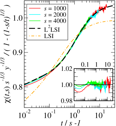
In figure 4, which gives a more fine appreciation of the shape of $f_{\chi}(y)$ than figure 2, we compare data for the reduced scaling function $f_{\rm red}(y)=f_{\chi}(y)y^{-1/3}\left[1-(1-y^{-1})^{1/3}\right]^{-1}$ with the predicted form (Phenomenology of ageing in the Kardar-Parisi-Zhang equation). Data with $s<10^{3}$ are not yet fully in the scaling regime. If one tries to fit the data with a non-logarithmic LSI (then $R=\langle\phi\widetilde{\phi}\rangle$ or $\langle\psi\widetilde{\phi}\rangle$) one obtains an agreement with the data, with a numerical precision of about 5%. An attempt to fit only with the first-order logarithmic terms (then $R=\langle\phi\widetilde{\psi}\rangle$) with $A_{2}=0$ assumed, gives back the same result, see table 2. Only if one uses the full structure of logarithmic LSI, an excellent representation of the data is found, to an accuracy better than $0.1\%$ over the range of data available. In the inset the ratio $\chi(t,s)/\chi_{\mbox{\rm\footnotesize L${}^{2}$LSI}}(t,s)$ is shown and we see that at least down to $t/s\approx 1.03$, the data collapse indicating dynamical scaling holds true, within the accuracy limits set by the stochastic noise, within $\approx 0.5\%$. For the largest waiting time $s=4000$, this observation entends over the entire range of values of $t/s$ considered. This indicates that the local height $h$ and its response field $\widetilde{h}$ of the $1D$ KPZ equation could be tentatively identified with the logarithmic quasi-primary operators $\psi$, $\widetilde{\psi}$, which slightly generalises the findings for the EW and MH classes, which obey non-logarithmic LSI. It is an open question whether the approach outlined here just generates the first two terms of an infinite logarithmic series in $R(t,s)$.

A systematic analysis of the invariance properties of the dynamical functionals studied for instance in Krec97 ; Lvov93 ; Frey96 , or the alternate form derived in Wio09 , would be of interest, following the lines of study for the analysis of dynamical symmetries in phase-ordering kinetics, see Henk10 and refs. therein.

	parameters
$R$	$a^{\prime}$	$A_{0}$	$A_{1}$	$A_{2}$
$\langle\phi\widetilde{\phi}\rangle$ – LSI	$-0.500$	$0.662$	0	0
$\langle\phi\widetilde{\psi}\rangle$ – L1LSI	$-0.500$	$0.663$	$-6\cdot 10^{-4}$	0
$\langle\psi\widetilde{\psi}\rangle$ – L2LSI	$-0.8206$	$0.7187$	$~{}~{}0.2424$	$-0.09087$

Table 2: Fitted parameters $A_{0,1,2}$ and $a^{\prime}$ used in figure 4.

Summarising, we tested the full scaling behaviour of simple ageing, both for correlators and responses, of systems in the $1D$ KPZ universality class. This is the first example of a growth process described by a non-linear equation which is shown to satisfy simple ageing scaling for space- and time-dependent quantities. It is non-trivial that the values of the growth and dynamical exponents, previously known from the study of the stationary state, are confirmed far from stationarity. It would be interesting to measure it also experimentally. Performing a numerical experiment, we find the form of the autoresponse scaling function to be very well described by the recently constructed logarithmic extension of local scale-invariance, with a natural identification of the leading quasi-primary operators. In view of important recent progress in the exact solution of the $1D$ KPZ equation, see Sasa10b ; Sasa10 ; Cala11 , one may expect that the question of a logarithmic dynamical scaling can be adressed and its further consequences explored.

This work was supported by the US National Science Foundation through DMR-0904999. This work was also supported by Mid-career Researcher Program through NRF grant No. 2011-0017982 funded by the Ministry of Education, Science, and Technology of Korea.

References

- (1) M. Kardar, G. Parisi and Y.-C. Zhang, Phys. Rev. Lett. 56, 889 (1986).
- (2) A.L. Barabási and H.E. Stanley, Fractal concepts in surface growth, Cambridge University Press (1995).
- (3) J. Krug, in A. McKane, M. Droz, J. Vannimenus and D. Wolf (Eds) Scale Invariance, Interfaces and Non-equilibrium Dynamics, NATO ASI, Vol. B344, Plenum (New York 1995); p. 1.
- (4) T. Halpin-Healy and Y.-C. Zhang, Phys. Rep. 254, 215 (1995).
- (5) T. Kriecherbauer and J. Krug, J. Phys. A43, 403001 (2010).
- (6) J. Krug, Adv. Phys. 46, 139 (1997).
- (7) T. Sasamoto and H. Spohn, J. Stat. Mech. P11013 (2010).
- (8) W.M. Tong and R.S. Williams, Ann. Rev. Phys. Chem. 45, 401 (1994).
- (9) M.T. Batchelor, R.V. Burne, B.I. Henry and S.D. Watt, Physica A282, 123 (2000).
- (10) T. Sasamoto and H. Spohn, Phys. Rev. Lett. 104, 230602 (2010).
- (11) P. Calabrese and P. Le Doussal, Phys. Rev. Lett. 106, 250603 (2011).
- (12) K.A. Takeuchi, M. Sano, T. Sasamoto and H. Spohn, Scientific Reports 1:34 (2011); K.A. Takeuchi and M. Sano, Phys. Rev. Lett. 104, 230601 (2010).
- (13) L.F. Cugliandolo, in JL Barrat et al. (eds) Slow relaxations and non-equilibrium dynamics in condensed matter, École de physique Les Houches LXXVII, Springer (Heidelbeg 2003).
- (14) M. Henkel and M. Pleimling, Non-equilibrium phase transitions, vol 2: Ageing and dynamical scaling far from equilibrium, Springer (Heidelberg 2010).
- (15) T. Enss, M. Henkel, A. Picone and U. Schollwöck, J. Phys. A37, 10479 (2004).
- (16) J.J. Ramasco, M. Henkel, M.A. Santos and C.A. da Silva Santos, J. Phys. A37, 10497 (2004).
- (17) G. Odor, J. Stat. Mech. L11002 (2006).
- (18) X. Durang, J.-Y. Fortin and M. Henkel, J. Stat. Mech. P02030 (2011).
- (19) F. Family and T. Vicsek, J. Phys. A18, L75 (1985).
- (20) S.F. Edwards and D.R. Wilkinson, Proc. Roy. Soc. A381, 17 (1982).
- (21) D.E. Wolf and J. Villain, Europhys. Lett. 13, 389 (1990).
- (22) A. Röthlein, F. Baumann and M. Pleimling, Phys. Rev. E74, 061604 (2006); E76, 019901(E) (2007).
- (23) H. Kallabis and J. Krug, Europhys. Lett. 45, 20 (1999).
- (24) G. L. Daquila and U. C. Täuber, Phys. Rev. E83, 051107 (2011).
- (25) S. Bustingorry, J. Stat. Mech. P10002 (2007); S. Bustingorry, L.F. Cugliandolo, and J.L. Iguain, J. Stat. Mech. P09008 (2007).
- (26) Y.-L. Chou and M. Pleimling, J. Stat. Mech. P08007 (2010).
- (27) In the EW and MH universality classes, one has . For the KPZ class is conjectured Kall99 .
- (28) T. J. Newman and M. R. Swift, Phys. Rev. Lett. 79, 2261 (1997).
- (29) J.M. Kim and J.M. Kosterlitz, Phys. Rev. Lett. 62, 2289 (1989).
- (30) M. Krech, Phys. Rev. E55, 668 (1997).
- (31) J.L. Iguain, S. Bustingorry, A.B. Kolton and L.F. Cugliandolo, Phys. Rev. B80, 094201 (2009).
- (32) U. Deker and F. Haake, Phys. Rev. A11, 2043 (1975); D. Forster, D.R. Nelson, and M.J. Stephen, Phys. Rev. A16, 732 (1977); E. Medina, T. Hwa, M. Kardar, and Y.-C. Zhang, Phys. Rev. A39, 3053 (1989).
- (33) V.S. L’vov, V.V. Lebedev, M. Paton, and I. Procaccia, Nonlinearity 6, 25 (1993).
- (34) E. Frey, U.C. Täuber, and T. Hwa, Phys. Rev. E53, 4424 (1996).
- (35) L. Canet, H. Chaté, B. Delamotte and N. Wschebor, Phys. Rev. Lett. 104, 150601 (2010).
- (36) M. Henkel, J. Phys. Cond. Matt. 19, 065101 (2007).
- (37) M. Henkel, J. Stat. Phys. 75, 1023 (1994).
- (38) M. Henkel and F. Baumann, J. Stat. Mech. P07015 (2007).
- (39) M. Henkel, T. Enss and M. Pleimling, J. Phys. A39, L589 (2006).
- (40) V. Gurarie, Nucl. Phys. B410, 535 (1993); M.R. Rahimi Tabar et al., Nucl. Phys. B497, 555 (1997); M.R. Gaberdiel and H.G. Kausch, Nucl. Phys. B538, 631 (1999); A. Hosseiny and S. Rouhani, J. Math. Phys. 51, 102303 (2010).
- (41) At equilibrium, percolation is a known case of logarithmic conformal invariance, P. Mathieu and D. Ridout, Nucl. Phys. B801, 268 (2008).
- (42) M. Henkel, arXiv:1009.4139v1 [hep-th].
- (43) H.S. Wio, Int. J. Bif. Chaos, 19, 2813 (2009).