Verification of Reynolds stress parameterizations from simulations

Abstract

We determine the timescales associated with turbulent diffusion and isotropization in closure models using anisotropically forced and freely decaying turbulence simulations and to study the applicability of these models. We compare the results from anisotropically forced three-dimensional numerical simulations with the predictions of the closure models and obtain the turbulent timescales mentioned above as functions of the Reynolds number. In a second set of simulations, turning the forcing off enables us to study the validity of the closures in freely decaying turbulence. Both types of experiments suggest that the timescale of turbulent diffusion converges to a constant value at higher Reynolds numbers. Furthermore, the relative importance of isotropization is found to be about 2.5 times larger at higher Reynolds numbers than in the more viscous regime.

1 Introduction

The dynamics of many astrophysical large-scale flows such as solar and stellar differential rotation are strongly controlled by velocity correlations at smaller scales. These correlations are referred to as components of the Reynolds stress tensor. It is well known that in rotating stratified convection the Reynolds stress tensor is anisotropic (Kippenhahn 1963), which then leads to the generation of differential rotation (Rüdiger et al. 1980, 1989). The Reynolds stress is defined as the average of products of components of velocity fluctuations, i.e., $R_{ij}=\overline{u_{i}u_{j}}$, where ${\bm{u}}={\bm{U}}-\overline{\vec{U}}$ is the fluctuation of the velocity ${\bm{U}}$ about its mean $\overline{\vec{U}}$. Here and in the following, overbars denote mean quantities, and for the purpose of this paper we shall restrict ourselves to volume averages.

Of particular interest are the equations governing the evolution of $R_{ij}$. In the astrophysical context, such model equations have been derived by Ogilvie (2003) and Garaud & Ogilvie (2005); see also Käpylä & Brandenburg (2008), Snellman et al. (2009), and Garaud et al. (2010). Such equations contain all the linear effects such as shear and rotation exactly. They usually also contain a driving term, $F_{ij}$, through which energy is injected into the system, as well as viscous and turbulent damping terms. Finally, there often is a term that describes, in a somewhat more ad-hoc fashion, the return to isotropy (Rotta 1951). The latter is important if the off-diagonal components happen to be different from zero due to some statistical perturbation. At least at the level of a thought experiment, one might ask how the system returns to isotropy after the effects that produced the anisotropy, e.g., rotation and stratification via the $\Lambda$-effect, have been turned off. Mathematically, the turbulent damping corresponds to terms involving triple correlations of the velocity while the term describing the return to isotropy comes from the interaction between components of velocity and those of gradients of the pressure with the velocity (Canuto 2009). Thus, in the absence of large-scale shear flows, rotation, gravity, or magnetic fields, we have

$$\dot{R}_{ij}=F_{ij}-\tau^{-1}R_{ij}-\tau_{\rm iso}^{-1}\left(R_{ij}-{\textstyle{1\over 3}}\delta_{ij}R\right),$$ (1)

where the dot denotes a time derivative, $R=R_{ii}$ is the trace of $R_{ij}$, while $\tau$ and $\tau_{\rm iso}$ are the relevant time scales describing turbulent diffusion and the return to isotropy.

Two very similar ways to characterizing these timescales have been proposed, both of which assume proportionality to the eddy turnover time, and $k_{\rm f}$ is the wavenumber of the energy-carrying eddies. $\tau_{\rm 0}=(u_{\rm rms}k_{\rm f})^{-1}$, where $u_{\rm rms}$ is the rms velocity. In the standard minimal $\tau$-approximation (hereafter MTA) (Blackman & Field, 2002, 2003) the return to isotropy is not accounted for, and $\tau$ is assumed constant in time. The value of $\tau$ can be expressed in terms of $\tau_{\rm 0}$ by defining a Strouhal number, ${\rm St}$, via

$$\tau={\rm St}\,\tau_{\rm 0}.$$ (2)

If the isotropization term is included in MTA, $\tau_{\rm iso}$ is, like $\tau$, also considered constant. In an approach used by Ogilvie (2003), the rms velocity is written as $u_{\rm rms}=R^{1/2}$, and dimensionless fit parameters are introduced to quantify $\tau$ and $\tau_{\rm iso}$:

$$\tau^{-1}=c_{1}k_{\rm f}R^{1/2},\quad\tau_{\rm iso}^{-1}=c_{2}k_{\rm f}R^{1/2}.$$ (3)

Besides the non-vanishing isotropization term, the main difference between these models is the nature of the eddy turnover time: in MTA it is usually constant, while in the Ogilvie approach it depends on the local and instantaneous value of $R$. The latter model can be thought of as an extension of the former to the case where $u_{\rm rms}$ varies.

There seems to be some diversity regarding the recommended choice of the coefficients $c_{1}$ and $c_{2}$. For the ratio $c_{1}/c_{2}$, Garaud & Ogilvie (2005) found the value 0.67, while in the additional presence of magnetic fields, Ogilvie (2003) found 0.87, and Liljeström et al. (2009) found 0.86. The work mentioned above has attempted to compute these coefficients as fit parameters in models where additional effects such as shear, rotation, and gravity are present. Such effects may however distort the results for $c_{1}$ and $c_{2}$, which characterize effects that are present even without the aforementioned processes.

A goal of this paper is to determine the two non-dimensional coefficients $c_{1}$ and $c_{2}$ using direct numerical simulations (DNS). We compute $c_{1}$ and $c_{2}$ here by imposing an anisotropic forcing term such that certain off-diagonal terms of its correlation matrix are non-vanishing. We use two independent methods to estimate the parameters: firstly, by comparing the steady state values for $R$ and $R_{ij}$ to the strength of the forcing, and secondly by observing the behavior of the system once the forcing is turned off, that is freely decaying turbulence. The predictions of the MTA and the Ogilvie approach regarding the behavior of the system in the latter case differ from one other, thus allowing us to assess the assumptions behind the two closures.

2 The model

We consider here a fully compressible gas with an isothermal equation of state for which the pressure $p$ is proportional to the density $\rho$ with $p=\rho c_{\rm s}^{2}$, where $c_{\rm s}={\rm const}{}$ is the isothermal sound speed. The computational domain is assumed Cartesian ${\bm{x}}=(x,y,z)$ with triply periodic boundary conditions. In some of our decay calculations, we start from a run where the Coriolis force is included, which is characterized by the angular velocity vector $\mbox{\boldmath$\Omega$}{}=(0,0,\Omega)$. The equation of motion and the continuity equation can then be written as

$${{\rm D}{}{\bm{U}}\over{\rm D}{}t}=-c_{\rm s}^{2}\mbox{\boldmath$\nabla$}{}\ln\rho-2\mbox{\boldmath$\Omega$}{}\times{\bm{U}}+{\bm{f}}+{1\over\rho}\mbox{\boldmath$\nabla$}{}\cdot(2\nu\rho\mbox{\boldmath${\sf S}$}{}),$$ (4)

$${{\rm D}{}\ln\rho\over{\rm D}{}t}=-\mbox{\boldmath$\nabla$}{}\cdot{\bm{U}},$$ (5)

where ${\rm D}{}/{\rm D}{}t=\partial/\partial t+{\bm{U}}\cdot\mbox{\boldmath$\nabla$}{}$ is the advective derivative, ${\sf S}_{ij}={\textstyle{1\over 2}}(U_{i,j}+U_{j,i})-{\textstyle{1\over 3}}\delta_{ij}\mbox{\boldmath$\nabla$}{}\cdot{\bm{U}}$ is the traceless rate of strain matrix, commas denote partial differentiation, $t$ is the time, and $\nu$ is the kinematic viscosity. The forcing term is an adaptation of a previously used (Brandenburg 2001) isotropic nonhelical forcing expression, ${\bm{f}}^{\rm iso}$, which is monochromatic with wavenumber ${\bm{k}}$, whose modulus lies in a narrow band around an average wavenumber $k_{\rm f}$, and the forcing is $\delta$-correlated in time such that ${\bm{k}}_{\rm f}(t)$ changes abruptly from one time step to the next. The isotropic forcing function is written as ${\bm{f}}=N{\bm{f}}_{{\bm{k}}}e^{{\rm i}{\bm{k}}(t)\cdot{\bm{x}}}$, where $N$ is a normalization factor, and ${\bm{f}}_{{\bm{k}}}=\hat{\bm{e}}\times{\bm{k}}$ (with random unit vector $\hat{\bm{e}}$) to ensure that the forcing is solenoidal. Both $\hat{\bm{e}}$ and ${\bm{k}}$ are random and non-parallel to each other. Next, we introduce a finite $xy$ correlation by writing the forcing term as

$${\bm{f}}={\bm{f}}^{\rm iso}+\sigma(\hat{\bm{x}}f^{\rm iso}_{y}+\hat{\bm{y}}f^{\rm iso}_{x}),$$ (6)

where $\hat{\bm{x}}$ and $\hat{\bm{y}}$ are unit vectors in the $x$ and $y$ directions, respectively, and $\sigma$ is a non-dimensional parameter measuring the degree of anisotropy. Note that

$$f_{x}f_{y}=(1+\sigma^{2})f^{\rm iso}_{x}f^{\rm iso}_{y}+\sigma[(f^{\rm iso}_{x})^{2}+(f^{\rm iso}_{y})^{2}],$$ (7)

and since $f^{\rm iso}_{x}f^{\rm iso}_{y}$ vanishes on the average, $f_{x}f_{y}$ has a positive definite mean. This then implies that in the Reynolds equations (1) the forcing tensor

$$F_{ij}=\rho(u_{i}f_{j}+u_{j}f_{i})$$ (8)

is also anisotropic with $F_{xy}\neq 0$ on the average.

To compute the effective timescales we consider steady state conditions in which case Eq. (1) implies

$$\tau^{-1}=\langle F\rangle/\langle R\rangle,$$ (9)

with $F=F_{ii}$ being the trace of $F_{ij}$, and

$$\tau^{-1}+\tau_{\rm iso}^{-1}=\langle F_{xy}\rangle/\langle R_{xy}\rangle,$$ (10)

where angle brackets now denote time averages.

A relevant control parameter is the Reynolds number, defined as

$$\mbox{\rm Re}=\frac{u_{\rm rms}}{\nu k_{\rm f}},$$ (11)

which is varied between 3 and 200. In some of the decay calculations that are initialized with rotation, we used a Coriolis number, $\mbox{\rm Co}=2\Omega/u_{\rm rms}k_{\rm f}$ of order unity. In all other cases we have $\mbox{\rm Co}=0$.

3 Results

We have produced three-dimensional DNS models with anisotropic forcing varying both the Reynolds number and also the effective wavenumber of the forcing, $k_{\rm f}$. Firstly, we determine $\tau^{-1}$ and $\tau^{-1}_{\rm iso}$ by comparing the steady state values for $R$ and $R_{ij}$ to the strength of the forcing in Sect. 3.1. In these experiments the numerical resolution is $256^{3}$ meshpoints. Secondly, we determine the inverse relaxation time scales from freely decaying turbulence in Sect. 3.2. Here, the numerical resolution is $128^{3}$ meshpoints.

3.1 Anisotropically forced turbulence

The inverse relaxation timescales $\tau^{-1}$ and $\tau^{-1}_{\rm iso}$ measured from anisotropically forced turbulence in a steady state with varying Reynolds number and effective forcing wavenumber are shown in Fig. 1. The results show a clear decline of $\tau^{-1}$ and $\tau^{-1}_{\rm iso}$ toward larger values Re. At the same time, $\tau^{-1}_{\rm iso}$ is about 2.5 times larger than $\tau^{-1}$, implying that $c_{1}/c_{2}\approx 0.4$, which is somewhat smaller than the values quoted in the literature; see Sect. 1.

Figure 1: Dependence of the inverse relaxation time scales (normalized by the dynamical value $\tau_{0}^{-1}$ on Re. Solid and dashed lines are for $\tau^{-1}$ and $\tau^{-1}_{\rm iso}$, respectively.

3.2 Decaying turbulence

In this section we deterime the value of the timescales $\tau$ and $\tau_{\rm iso}$ and obtain another estimate for these parameters by studying freely decaying turbulence. We also compare the validity of the assumptions behind MTA and the Ogilvie approach, since the closures predict decay behaviors that are different in the two cases. By letting the turbulence first achieve a saturated state and then turning off the forcing in our DNS we get a time series that can be compared with the predictions of the closure models. From Eq. (1) we can easily derive the time evolution equation for the trace of the Reynolds tensor by summing over the diagonal components:

$$\dot{R}=F-\tau^{-1}R,$$ (12)

where the summation causes the contribution from the isotropization term to vanish. Let the forcing be set to zero at $t=t_{0}$ and let $R(t_{0})=R^{(0)}$. If $\tau^{-1}$ is assumed constant in MTA, this approach predicts exponential decay. By integrating Eq. (12) in this case we have

$$R=R^{(0)}e^{-(t-t_{0})/\tau}.$$ (13)

The Ogilvie approach, however, predicts inverse square-type decay:

$$R=\left[\frac{1}{\sqrt{R^{(0)}}}+\frac{1}{2}c_{1}k_{f}(t-t_{0})\right]^{-2}.$$ (14)

Table 1: The model parameters $c_{1}$, $c_{2}$, $\tau^{-1}$ and $\tau_{\rm iso}^{-1}$ obtained from the DNS of freely decaying turbulence. The superscripts $b$ and $l$ refer to the beginning and the late parts of the time series.

$$\begin{array}[]{p{0.06\linewidth}ccccccccrrr}\hline\cr\vskip 3.0pt plus 1.0pt minus 1.0pt\cr Run&k_{\rm f}/k_{\rm 1}&\rm Re&\tau^{-1}/\tau_{0}^{-1}&c_{1}^{b}&c_{1}^{l}&\tau_{\rm iso}^{-1}/\tau_{0}^{-1}&c_{2}^{b}&c_{2}^{l}\\ \vskip 3.0pt plus 1.0pt minus 1.0pt\cr\hline\cr L1&3&53&0.11&0.12&0.16&0.08&0.14&-\\ L2&3&55&0.11&0.12&0.16&-&-&-\\ L3&3&61&0.12&0.14&0.16&-&-&-\\ L4&3&79&0.12&0.14&0.17&0.04&0.07&-\\ L5&1.5&147&0.08&0.09&0.15&-&-&-\\ L6&10&14&0.19&0.23&0.27&0.06&0.08&-\\ L7&10&32&0.13&0.15&0.18&-&-&-\\ L8&3&113&0.11&0.13&0.16&0.08&0.08&-\\ L9&3&191&0.10&0.11&0.15&0.06&0.10&-\\ \vskip 3.0pt plus 1.0pt minus 1.0pt\cr\hline\cr F1&3&24&0.19&0.21&0.25&0.13&0.15&-\\ F2&3&53&0.13&0.13&0.19&0.19&0.23&0.05\\ F3&3&92&0.13&0.14&0.18&0.27&0.27&0.07\\ F4&1.5&55&0.13&0.15&0.25&0.32&0.32&-\\ F5&1.5&115&0.12&0.13&0.22&0.31&0.31&0.12\\ F6&1.5&192&0.12&0.13&0.20&0.10&0.11&0.04\\ F7&10&5&0.44&0.48&0.65&0.09&0.23&-\\ F8&10&13&0.23&0.27&0.32&0.13&0.15&-\\ F9&10&24&0.16&0.18&0.24&0.17&0.17&-\\ \end{array}$$

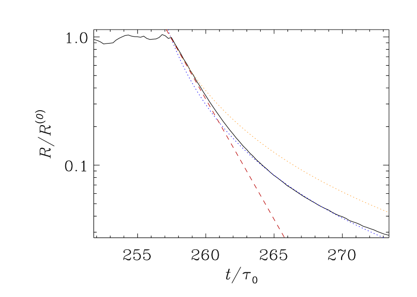
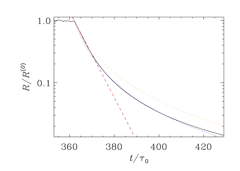
By plotting Eqs. (13) and (14) with the time series from DNS the behavior of the closures can be tested and the model parameters $c_{1}$ and $\tau$ estimated. We have performed two sets of runs, the results of which are summarized in Table 1. In Set F, we use the forcing scheme described in Sect. 2, while the runs in Set L were made using anisotropic, nonhelical forcing in combination with rotation ($\Omega\neq 0$ to) produce off-diagonal Reynolds stress components through the $\Lambda$-effect; see Käpylä & Brandenburg (2008) for a detailed description). The values listed in the table were obtained by fitting Eqs. (13) and (14) to the DNS results. Two examples of such a fit can be seen in Fig. 2. The solid lines represent the DNS data, the dashed red lines the decay behavior predicted by the MTA. The yellow and blue dotted lines are the corresponding prediction of the Ogilvie closure with two different values for $c_{1}$, denoted with $c^{b}_{1}$ and $c^{l}_{1}$ for the determination of which the beginning and later parts of the DNS time series was used, respectively. The two alternative fits for the latter model have been introduced because of the changing nature of the process. As we can see, the decay generally follows the exponential pattern at first, but in the later stages power-law behavior similar to the prediction of the Ogilvie model takes place. However, eventually the DNS results move away from both predictions.

Figure 2: The time evolution of $R$ in freely decaying turbulence. Dotted and dashed lines show the decay predictions of the Ogilvie model and MTA, respectively, with suitable values for $c_{1}$ and $\tau$ , and the solid line is the DNS time series. The upper panel shows the results from Run F7 and lower panel results from Run F9.

This kind of changing behavior is observed in all of the decay models, and the temporal span of the validity of various predictions vary between the runs. This can be seen in Fig. 2, in which the upper panel shows the fit to the DNS data from Run F7, and the lower panel shows a corresponding fit to the data from Run F9: while the exponential prediction of MTA seems to apply for approximately the same duration in both panels, the Ogilvie approach has clearly a different range of applicability. Table 1 lists the different fit parameters $c^{b}_{1}$, $c^{l}_{1}$ and $\tau^{-1}/\tau_{0}^{-1}$ obtained from the decay models. The values for $c^{b}_{1}$ are generally very close to the values of $\tau^{-1}/\tau_{0}^{-1}$, while $c^{l}_{1}$ tend to be somewhat larger. Actually, if one puts $c_{1}=\tau^{-1}/\tau_{0}^{-1}$, the resulting curve has MTA prediction as a tangent at $t_{0}$.

Parameters $\tau_{\rm iso}$ and $c_{2}$ can be estimated by studying the decay of the off-diagonal components of the Reynolds stress. The time evolution equation for $R_{ij}$ in the forced non-diagonal case reads

$$\dot{R}_{ij}=F_{ij}-(\tau^{-1}+\tau_{\rm iso}^{-1})R_{ij}.$$ (15)

Now, let $R_{ij}(t_{0})=R_{ij}^{(0)}$. Assuming $\tau_{\rm iso}$ constant in the case of MTA we have again exponential decay:

$$R_{ij}=R_{ij}^{(0)}e^{-(t-t_{0})(\tau^{-1}+\tau_{\rm iso}^{-1})}.$$ (16)

To get the corresponding result for the Ogilvie model one needs to use Eq. (14) to solve for $\sqrt{R}$ and integrate over time. The final result reads

$$R_{ij}=R_{ij}^{(0)}\left[1+\frac{\sqrt{R^{(0)}}}{2}c_{1}k_{\rm f}(t-t_{0})\right]^{-2\frac{c_{1}+c_{2}}{c_{1}}}.$$ (17)

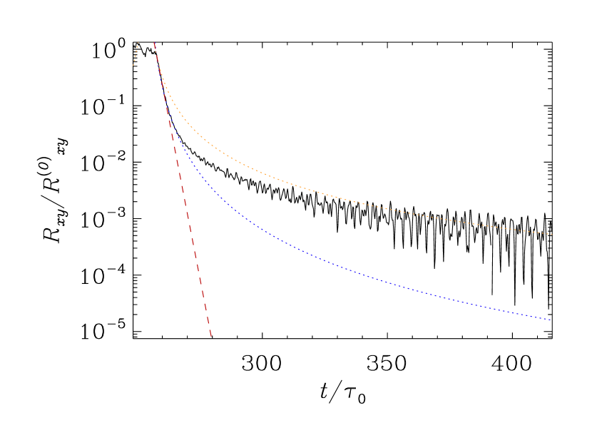
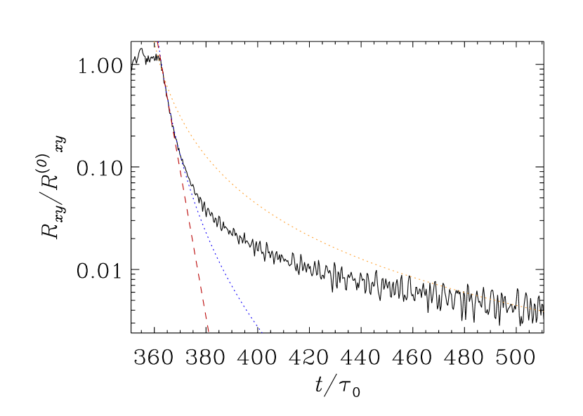
The DNS results are compared with the predictions from the closure models in Fig. 3. Again we show two alternative versions for the behavior of the Ogilvie model with different values for $c_{2}$, $c_{2}^{b}$ and $c_{2}^{l}$, with the same reasoning as with $c_{1}$. According to Eqs. (16) and (17), the decay of $R_{xy}$ depends on the relaxation parameters $\tau$ and $c_{1}$ as well as the dedicated isotropization parameters $\tau_{\rm iso}$ and $c_{2}$. Using the estimates for the relaxation terms obtained from the decay of $R$ we can determine the isotropization terms by treating them as the only free parameters of the models and finding a reasonable fit, like before. In the case of $c_{2}$ we have used the initial value $c_{1}^{b}$ for this purpose.

Figure 3: The time evolution of $R_{xy}$ in freely decaying turbulence. Dotted and dashed lines show the decay prediction of the Ogilvie model and MTA, respectively, with suitable values for $c_{2}$ and $\tau$ , and the solid line is the DNS time series. The runs displayed are the same as in Fig. 2.

The results for the isotropization terms are summarized in Table 1. A problem in many runs is that the fluctuations of the off-diagonal components of the Reynolds stresses can be larger than their average value, causing their sign to change frequently. In the decay phase the time series of these runs tend to contain strong oscillations right from the beginning. The oscillations are similar to what can be seen in Fig. 3, and they make finding an unambiguous fit very challenging. In some cases a suitable fit would have required negative values for the parameter $c_{2}$. For these cases, no value is given in Table 1. This problem manifests itself mostly in Set L. Thus, the most reliable results come from Set F, where $R_{xy}$ get non-zero mean values more consistently, and fluctuations are not too large. We see that $\tau_{\rm iso}^{-1}/\tau_{0}^{-1}$ and $c_{2}^{b}$ obtain very similar values, while $c_{2}^{l}$ is mostly very small or zero. Equation (17) implies that with $c_{2}=0$ the decay of the off-diagonal components of the Reynolds stresses should behave like the decay of $R$ described by Eq. (14), so the vanishing of $c_{2}^{l}$ may indicate the isotropization switching off. But then again, it is seen in Fig. 3 that even with vanishing $c_{2}$ the prediction becomes gradually worse as time progresses, and in the lower panel the period of validity is restricted to a brief intersection. Large fluctuations are another source of ambiguity near the end of the time series.

Figure 4 contains the same results as Fig. 1, but obtained for the decay models. Due to the ambiguity of the results from the Set L, only results from Set F are shown for $\tau_{\rm iso}^{-1}$. In both figures the overall trend is similar: $\tau^{-1}$ is large with small Reynolds numbers, and decreases as Re increases. Unlike in Fig. 1, in Fig. 4 $\tau_{\rm iso}^{-1}$ generally increases with increasing Re, and eventually becomes greater than $\tau^{-1}$. It would seem that the results for $\tau^{-1}$ approach some constant value at high Reynolds numbers, but more simulations with higher Reynolds numbers would be needed to verify this. Increasing $\tau^{-1}$ with decreasing Re may explain, why the nature of the decline of $R$ changes in the decay models. If we take $u_{\rm rms}=R^{1/2}$ in the decay phase, the effective Reynolds numbers falls accordingly. This would mean that $\tau^{-1}$ changes during the simulation, leading to a different behavior.

Figure 4: Inverse relaxation time scales (normalized by the dynamical value $\tau_{0}^{-1}$) as functions of Re obtained from the decay models. Dotted and dashed lines are for $\tau^{-1}$ and $\tau^{-1}_{\rm iso}$, respectively. The diamonds represent runs with $k_{\rm f}/k_{\rm 1}=1.5$, triangles $k_{\rm f}/k_{\rm 1}=3$ and asterisks $k_{\rm f}/k_{\rm 1}=10$.

4 Conclusions

In this study we have investigated anisotropically forced hydrodynamic turbulence, and determined the timescales related to the diffusion and isotropization processes from our DNS models. The obtained results were compared to two different closure model predictions, namely the minimal tau approximation and the Ogilvie approach.

Our results from the steady-state forced turbulence models show that the values of $\tau^{-1}$, describing the diffusion process, and $\tau^{-1}_{\rm iso}$, describing the isotropization process, depend on Re for small and intermediate values, but show clear signs of convergence for larger values. In particular, it turns out that $\tau^{-1}_{\rm iso}$ is clearly larger than $\tau^{-1}$, and that their inverse ratio is around 0.4, which is somewhat less than the results published earlier in the literature.

Our models of freely decaying turbulence show that, while the decay is exponential at first, as predicted by the MTA with a constant $\tau$, it deviates from this pattern in the later stages, following a power-law behavior much like the one predicted by the Ogilvie approach. Finally also the Ogilvie prediction breaks down far away from the switch-off point of the forcing.