Statistical-physics-based reconstruction in compressed sensing
Abstract
Compressed sensing is triggering a major evolution in signal acquisition. It consists in sampling a sparse signal at low rate and later using computational power for its exact reconstruction, so that only the necessary information is measured. Currently used reconstruction techniques are, however, limited to acquisition rates larger than the true density of the signal. We design a new procedure which is able to reconstruct exactly the signal with a number of measurements that approaches the theoretical limit in the limit of large systems. It is based on the joint use of three essential ingredients: a probabilistic approach to signal reconstruction, a message-passing algorithm adapted from belief propagation, and a careful design of the measurement matrix inspired from the theory of crystal nucleation. The performance of this new algorithm is analyzed by statistical physics methods. The obtained improvement is confirmed by numerical studies of several cases.
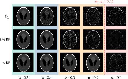
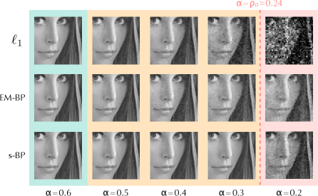
The ability to recover high dimensional signals using only a limited number of measurements is crucial in many fields, ranging from image processing to astronomy or systems biology. Example of direct applications include speeding up magnetic resonance imaging without the loss of resolution, sensing and compressing data simultaneously Candès & Wakin (2008) and the single-pixel camera Duarte et al. (2008). Compressed sensing is designed to directly acquire only the necessary information about the signal. This is possible when the signal is sparse in some known basis. In a second step one uses computational power to reconstruct the signal exactly Candès & Tao (2005); Donoho (2006); Candès & Wakin (2008). Currently, the best known generic method for exact reconstruction is based on converting the reconstruction problem into a convex optimization one, which can be solved efficiently using linear programming techniques Candès & Tao (2005); Donoho (2006). The reconstruction is able to reconstruct accurately, provided the system size is large and the ratio of the number of measurements to the number of non-zeros exceeds a specific limit which can be proven by careful analysis Donoho & Tanner (2005); Donoho (2006). However, the limiting ratio is significantly larger than . In this paper we improve on the performance of minimization, and in the best possible way: we introduce a new procedure that is able to reach the optimal limit . This procedure, which we call seeded Belief Propagation (s-BP) is based on a new, carefully designed, measurement matrix. It is very powerful, as illustrated in Fig. 1. Its performance will be studied here with a joint use of numerical and analytic studies using methods from statistical physics Mézard et al. (1987).
Reconstruction in Compressed Sensing
The mathematical problem posed in compressed-sensing reconstruction is easily stated. Given an unknown signal which is a -dimensional vector s, we make measurements, where each measurement amounts to a projection of s on some known vector. The measurements are grouped into a -component vector y, which is obtained from s by a linear transformation . Depending on the application, this linear transformation can be for instance associated with measurements of Fourier modes or wavelet coefficients. The observer knows the matrix F and the measurements y, with . His aim is to reconstruct s. This is impossible in general, but compressed sensing deals with the case where the signal s is sparse, in the sense that only of its components are non-zero. We shall study the case where the non-zero components are real numbers and the measurements are linearly independent. In this case, exact signal reconstruction is possible in principle whenever , using an exhaustive enumeration method which tries to solve for all possible choices of locations of non-zero components of x: only one such choice gives a consistent linear system, which can then be inverted. However, one is typically interested in large instances where , with and . The enumeration method solves the compressed sensing problem in the regime where measurement rates are at least as large as the signal density, , but in a time which grows exponentially with , making it totally impractical. Therefore is the fundamental reconstruction limit for perfect reconstruction in the noiseless case, when the non-zero components of the signal are real numbers drawn from a continuous distribution. A general and detailed discussion of information-theoretically optimal reconstruction has been developed recently in Wu & Verdu (2011a, b); Guo et al. (2009).
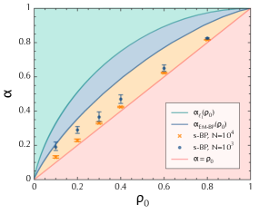
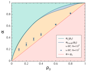
In order to design practical ‘low-complexity’ reconstruction algorithms, it has been proposed Candès & Tao (2005); Donoho (2006) to find a vector x which has the smallest norm, , within the subspace of vectors which satisfy the constraints , using efficient linear programming techniques. In order to measure the performance of this strategy one can focus on the measurement matrix F generated randomly, with independent Gaussian-distributed matrix elements of mean zero and variance , and the signal vector s having density . The analytic study of the reconstruction in the thermodynamic limit can be done using either geometric or probabilistic methods Donoho & Tanner (2005); Donoho et al. (2009), or with the replica method Kabashima et al. (2009); Rangan et al. (2009); Ganguli & Sompolinsky (2010). It shows the existence of a sharp phase transition at a value . When is larger than this value, the reconstruction gives the exact result with probability going to one in the large limit, when the probability that it gives the exact result goes to zero. As shown in Fig. 2, and therefore the reconstruction is suboptimal: it requires more measurements than would be absolutely necessary, in the sense that, if one were willing to do brute-force combinatorial optimization, no more than measurements are necessary.
We introduce a new measurement and reconstruction approach, s-BP, that allows to reconstruct the signal by a practical method, which needs only measurements. We shall now discuss its three ingredients: 1) a probabilistic approach to signal reconstruction, 2) a message-passing algorithm adapted from belief propagation Pearl (1982), which is a procedure known to be efficient in various hard computational problems Richardson & Urbanke (2008); Mézard & Montanari (2009), and 3) an innovative design of the measurement matrix inspired from the theory of crystal nucleation in statistical physics and from recent developments in coding theory Jimenez Felstrom & Zigangirov (1999); Kudekar et al. (2010); Lentmaier & Fettweis (2010); Hassani et al. (2010). Some previous works on compressed sensing have used these ingredients separately. In particular, adaptations of belief propagation have been developed for the compressed sensing reconstruction, both in the context of reconstruction Donoho et al. (2009, 2010); Rangan (2011), and in a probabilistic approach Rangan (2010). The idea of seeding matrices in compressed sensing was introduced in KudekarPfister (2010). It is however only the combined use of these three ingredients that allows us to reach the limit.
A probabilistic approach
For the purpose of our analysis, we consider the case where the signal s has independent identically distributed (iid) components: , with . In the large- limit the number of non-zero components is . Our approach handles general distributions .
Instead of using a minimization procedure, we shall adopt a probabilistic approach. We introduce a probability measure over vectors which is the restriction of the Gauss-Bernoulli measure to the subspace Note1 (26). In this paper, we use a distribution which is a Gaussian with mean and variance , but other choices for are possible. It is crucial to note that we do not require a priori knowledge of the statistical properties of the signal: we use a value of not necessarily equal to , and the that we use is not necessarily equal to . The important point is to use (which reflects the fact that one searches a sparse signal).
Assuming that F is a random matrix, either where all the elements are drawn as independent Gaussian random variables with zero mean and the same variance, or of the carefully-designed type of ‘seeding matrices’ described below, we demonstrate in Appendix A that, for any -dense original signal s, and any the probability of the original signal goes to one when . This result holds independently of the distribution of the original signal, which does not need to be known. In practice, we see that s also dominates the measure when is not very large. In principle, sampling configurations x proportionally to the restricted Gauss-Bernoulli measure thus gives asymptotically the exact reconstruction in the whole region . This idea stands at the roots of our approach, and is at the origin of the connection with statistical physics (where one samples with the Boltzmann measure).
Sampling with Expectation Maximization Belief Propagation
The exact sampling from a distribution such as , eq. (2), is known to be computationally intractable Natarajan (1995). However, an efficient approximate sampling can be performed using a message-passing procedure that we now describe Thouless et al. (1977); Tanaka (2002); Guo & Wang (2006); Rangan (2010). We start from the general belief-propagation formalism Kschischang et al. (2001); Yedidia et al. (2003); Mézard & Montanari (2009): for each measurement and each signal component , one introduces a ‘message’ which is the probability of in a modified measure where measurement has been erased. In the present case, the canonical belief propagation equations relating these messages can be simplified Donoho et al. (2009, 2010); Rangan (2010, 2011); Montanari & Bayati (2011) into a closed form that uses only the expectation and the variance of the distribution (see Appendix B). An important ingredient that we add to this approach is the learning of the parameters in : the density , and the mean and variance of the Gaussian distribution . These are three parameters to be learned using update equations based on the gradient of the so-called Bethe free entropy, in a way analogous to the expectation maximization Dempster et al. (1977); Iba (1999); Decelle et al. (2011). This leads to the Expectation Maximization Belief Propagation (EM-BP) algorithm that we will use in the following for reconstruction in compressed sensing. It consists in iterating the messages and the three parameters, starting from random messages and , until a fixed point is obtained. Perfect reconstruction is found when the messages converge to the fixed point and .
Like the reconstruction, the EM-BP reconstruction also has a phase transition. Perfect reconstruction is achieved with probability one in the large- limit if and only if . Using the asymptotic replica analysis, as explained below, we have computed the line when the elements of the measurement matrix F are independent Gaussian random variables with zero mean and variance and the signal components are iid. The location of this transition line does depend on the signal distribution, see Fig. 2, contrary to the location of the phase transition.
Notice that our analysis is fully based on the case when the probabilistic model has a Gaussian . Not surprisingly, EM-BP performs better when , see the left-hand side of Fig. 2, where EM-BP provides a sizable improvement over . In contrast, the right-hand side of Fig. 2 shows an adversary case when we use a Gaussian to reconstruct a binary , in this case there is nearly no improvement over reconstruction.
Designing seeding matrices
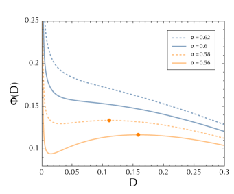
In order for the EM-BP message-passing algorithm to be able to reconstruct the signal down to the theoretically optimal number of measurements , one needs to use a special family of measurement matrices F that we call ‘seeding matrices’. If one uses an unstructured F, for instance a matrix with independent Gaussian-distributed random elements, EM-BP samples correctly at large , but at small enough a metastable state appears in the measure , and the EM-BP algorithm is trapped in this state, and is therefore unable to find the original signal (see Fig. 3), just as a supercooled liquid gets trapped in a glassy state instead of crystallizing. It is well known in crystallization theory that the crucial step is to nucleate a large enough seed of crystal. This is the purpose of the following design of F.
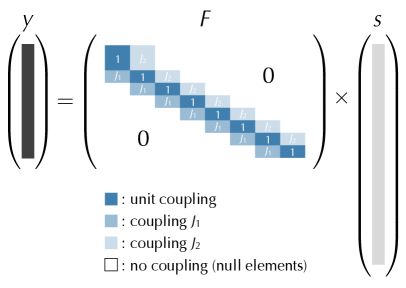
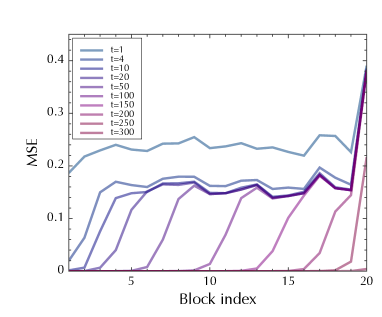
We divide the variables into groups of variables, and the measurements into groups. The number of measurements in the -th group is , so that . We then choose the matrix elements independently, in such a way that, if belongs to group and to group then is a random number chosen from the normal distribution with mean zero and variance (see Fig. 4). The matrix is a coupling matrix (and the standard compressed sensing matrices are obtained using and ). Using these new matrices, one can shift the BP phase transition very close to the theoretical limit. In order to get an efficient reconstruction with message passing, one should use a large enough . With a good choice of the coupling matrix , the reconstruction first takes place in the first block, and propagates as a wave in the following blocks , even if their measurement rate is small. In practice, we use , so that the total measurement rate is . The whole reconstruction process is then analogous to crystal nucleation, where a crystal is growing from its seed (see Fig. 5). Similar ideas have been used recently in the design of sparse coding matrices for error-correcting codes Jimenez Felstrom & Zigangirov (1999); Kudekar et al. (2010); Lentmaier & Fettweis (2010); Hassani et al. (2010).
Analysis of the performance of the seeded Belief Propagation procedure
The s-BP procedure is based on the joint use of seeding measurement matrices and of the EM-BP message-passing reconstruction. We have studied it with two methods: direct numerical simulations and analysis of the performance in the large limit. The analytical result was obtained by a combination of the replica method and of the cavity method (also known as ‘density evolution’ or ‘state evolution’). The replica method is a standard method in statistical physics Mézard et al. (1987), which has been applied successfully to several problems of information theory Nishimori (2001); Tanaka (2002); Guo & Verdú (2005); Mézard & Montanari (2009) including compressed sensing Rangan et al. (2009); Kabashima et al. (2009); Ganguli & Sompolinsky (2010). It can be used to compute the free entropy function associated with the probability (see Appendix D), and the cavity method shows that the dynamics of the message-passing algorithm is a gradient dynamics leading to a maximum of this free-entropy.
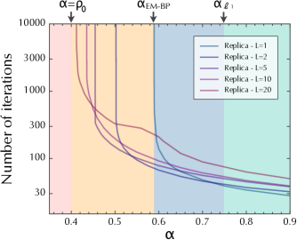
When applied to the usual case of the full F matrix with independent Gaussian-distributed elements (case ), the replica computation shows that the free-entropy for configurations constrained to be at a mean-squared distance has a global maximum at when , which confirms that the Gauss-Bernoulli probabilistic reconstruction is in principle able to reach the optimal compression limit . However, for , where is a threshold that depends on the signal and on the distribution , a secondary local maximum of appears at (see Fig. 3). In this case the EM-BP algorithm converges instead to this secondary maximum and does not reach exact reconstruction. The threshold is obtained analytically as the smallest value of such that is decreasing (Fig. 2). This theoretical study has been confirmed by numerical measurements of the number of iterations needed for EM-BP to reach its fixed point (within a given accuracy). This convergence time of BP to the exact reconstruction of the signal diverges when (see Fig. 3). For the EM-BP algorithm converges to a fixed point with strictly positive mean-squared error (MSE). This ‘dynamical’ transition is similar to the one found in the cooling of liquids which go into a super-cooled glassy state instead of crystallizing, and appears in the decoding of error correcting codes Richardson & Urbanke (2008); Mézard & Montanari (2009) as well.
We have applied the same technique to the case of seeding-measurement matrices (). The cavity method allows to analytically locate the dynamical phase transition of s-BP. In the limit of large , the MSE and the variance messages in each block , the density , the mean , and the variance of evolve according to a dynamical system which can be computed exactly (see Appendix E), and one can see numerically if this dynamical system converges to the fixed point corresponding to exact reconstruction ( for all ). This study can be used to optimize the design of the seeding matrix F by choosing , and in such a way that the convergence to exact reconstruction is as fast as possible. In Fig. 3 we show the convergence time of s-BP predicted by the replica theory for different sets of parameters. For optimized values of the parameters, in the limit of a large number of blocks , and large system sizes , s-BP is capable of exact reconstruction close to the smallest possible number of measurements, . In practice, finite size effects slightly degrade this asymptotic threshold saturation, but the s-BP algorithm nevertheless reconstructs signals at rates close to the optimal one regardless of the signal distribution, as illustrated in Fig. 2.
We illustrate the evolution of the s-BP algorithm in Fig. 5. The non-zero signal elements are Gaussian with zero mean, unit variance, density and measurement rate , which is deep in the glassy region where all other known algorithms fail. The s-BP algorithm first nucleates the native state in the first block and then propagates it through the system. We have also tested the s-BP algorithm on real images where the non-zero components of the signal are far from Gaussian, and the results are nevertheless very good, as shown in Fig. 1. This shows that the quality of the result is not due to a good guess of . It is also important to mention that the gain in performance in using seeding-measurement matrices is really specific to the probabilistic approach: we have computed the phase diagram of minimization with these matrices and found that, in general, the performance is slightly degraded with respect to the one of the full measurement matrices, in the large limit. This demonstrates that it is the combination of the probabilistic approach, the message-passing reconstruction with parameter learning, and the seeding design of the measurement matrix that is able to reach the best possible performance.
Perspectives
The seeded compressed sensing approach introduced here is versatile enough to allow for various extensions. One aspect worth mentioning is the possibility to write the EM-BP equations in terms of messages instead of the parameters as described in Appendix C. This is basically the step that goes from rBP Rangan (2010) to AMP Donoho et al. (2009) algorithm. It could be particularly useful when the measurement matrix has some special structure, so that the measurements y can be obtained in many fewer than operations (typically in operations). We have also checked that the approach is robust to the introduction of a small amount of noise in the measurements (see Appendix H). Finally, let us mention that, in the case where a priori information on the signal is available, it can be incorporated in this approach through a better choice of , and considerably improve the performance of the algorithm. For signal with density , the worst case, that we addressed here, is when the non-zero components of the signal are drawn from a continuous distribution. Better performance can be obtained with our method if these non-zero components come from a discrete distribution and one uses this distribution in the choice of . Another interesting direction in which our formalism can be extended naturally is the use of non-linear measurements and different type of noises. Altogether, this approach turns out to be very efficient both for random and structured data, as illustrated in Fig. 1, and offers an interesting perspective for fpractical compressed sensing applications. Data and code are available online at noteASPICS (7).
Acknowledgements We thank Y. Kabashima, R. Urbanke and specially A. Montanari for useful discussions. This work has been supported in part by the EC grant ‘STAMINA’, No 265496, and by the grant DySpaN of ‘Triangle de la Physique’.
Note: During the review process for our paper, we became aware of the work Donoho et al. (2011) in which the authors give a rigorous proof of our result, in the special case when and , that the threshold can be reached asymptotically by the s-BP procedure.
Appendix A Proof of the optimality of the probabilistic approach
Here we give the main lines of the proof that our probabilistic approach is asymptotically optimal. We consider the case where the signal s has iid components
| (1) |
with . And we study the probability distribution
| (2) |
with a Gaussian of mean zero and unit variance. We stress here that we consider general , i.e. is not necessarily equal to (and is not necessarily equal to ). The measurement matrix F is composed of iid elements such that if belongs to block and belongs to block then is a random number generated from the Gaussian distribution with zero mean and variance /N. The function is a centered Gaussian distribution with variance .
We show that, with probability going to one in the large limit (at fixed ), the measure (obtained with a generic seeding matrix F as described in the main text) is dominated by the signal if , (as long as is finite).
We introduce the constrained partition function:
| (3) |
and the corresponding ‘free entropy density’: . The notations and denote respectively the expectation value with respect to F and to s. denotes an indicator function, equal to one if its argument is true, and equal to zero otherwise.
The proof of optimality is obtained by showing that, under the conditions above, is finite if (statement 1), and it vanishes if (statement 2). This proves that the measure is dominated by , i.e. by the neighborhood of the signal . The standard ‘self-averageness’ property, which states that the distribution (with respect to the choice of F and s) of concentrates around when , completes the proof. We give here the main lines of the first two steps of the proof.
We first sketch the proof of statement 2. The fact that when can be derived by a first moment bound:
| (4) |
where is the ‘annealed partition function’ defined as
| (5) |
In order to evaluate one can first compute the annealed partition function in which the distances between and the signal are fixed in each block. More precisely, we define
By noticing that the random variables are independent Gaussian random variables one obtains:
| (6) |
where
| (7) |
The behaviour of is easily obtained by standard saddle point methods. In particular, when , one has .
Using (6), we obtain, in the small limit:
| (8) |
where the maximum over is to be taken under the constraint . Taking the limit of with a finite , at least one of the distance must remain finite. It is then easy to show that
| (9) |
where is the fraction of measurements in blocks to . As , this is less singular than , which proves statement 2.
On the contrary, when , we obtain from the same analysis
| (10) |
This annealed estimate actually gives the correct scaling at small , as can be shown by the following lower bound. When , we define as the subset of indices where , , and as the subset of indices where , . We obtain a lower bound on by substituting by the factors when and when . This gives:
| (11) | |||||
where . The matrix , of size , is a Wishart-like random matrix. For , generically, its eigenvalues are strictly positive, as we show below. Using this property, one can show that, if , the integral over the variables in (11) is strictly positive in the limit . The divergence of in the limit is due to the explicit term in Eq. (11).
The fact that all eigenvalues of are strictly positive is well known in the case of where the spectrum has been obtained by Marcenko and Pastur. In general, the fact that all the eigenvalues of are strictly positive is equivalent to saying that all the lines of the matrix (which is the restriction of the measurement matrix to columns with non-zero signal components) are linearly independent. In the case of seeding matrices with general , this statement is basically obvious by construction of the matrices, in the regime where in each block , and . A more formal proof can be obtained as follows. We consider the Gaussian integral
| (12) |
This quantity is finite if and only if is smaller than the smallest eigenvalue, , of . We now compute the annealed average . If is finite, then the probability that goes to zero in the large N limit. Using methods similar to the one above, one can show that
| (13) |
The saddle point equations
| (14) |
have a solution at (and by continuity also at small enough), when (it can be found for instance by iteration). Therefore, is finite for some small enough, and therefore .
Appendix B Derivation of Expectation maximization Belief Propagation
In this and the next sections we present the message-passing algorithm that we used for reconstruction in compressed sensing. In this section we derive its message-passing form, where messages are being sent between each signal component and each measurement . This algorithm was used in Rangan (2010), where it was called the relaxed belief propagation, as an approximate algorithm for the case of a sparse measurement matrix F. In the case that we use here of a measurement matrix which is not sparse (a finite fraction of the elements of F is non-zero, and all the non-zero elements scale as ), the algorithm is asymptotically exact. We show here for completeness how to derive it. In the next section we then derive asymptotically equivalent equations that depend only on messages. In statistical physics terms, this corresponds to the TAP equations Thouless et al. (1977) with the Onsager reaction term, that are asymptotically equivalent to the BP on fully connected models. In the context of compressed sensing this form of equations has been used previously Donoho et al. (2009) and it is called approximate message passing (AMP). In cases when the matrix F can be computed recursively (e.g. via fast Fourier transform), the running time of the AMP-type message passing is (compared to the for the non-AMP form). Apart for this speed-up, both classes of message passing give the same performance.
We derive here the message-passing algorithm in the case where measurements have additive Gaussian noise, the noiseless case limit is easily obtained in the end. The posterior probability of x after the measurement of y is given by
| (15) |
where is a normalization constant (the partition function) and is the variance of the noise in measurement . The noiseless case is recovered in the limit . The optimal estimate, that minimizes the MSE with respect to the original signal s, is obtained from averages of with respect to the probability measure . Exact computation of these averages would require exponential time, belief propagation provides a standard approximation. The canonical BP equations for probability measure read
| (16) | |||||
| (17) |
where and are normalization factors ensuring that . These are integral equations for probability distributions that are still practically intractable in this form. We can, however, take advantage of the fact that after proper rescaling the linear system is such a way that elements of y and x are of , the matrix has random elements with variance of . Using the Hubbard-Stratonovich transformation
| (18) |
for we can simplify eq. (16) as
| (19) |
Now we expand the last exponential around zero because the term is small in , we keep all terms that are of . Introducing means and variances as new messages
| (20) | |||||
| (21) |
we obtain
| (22) |
Performing the Gaussian integral over we obtain
| (23) |
where we introduced
| (24) | |||||
| (25) |
and the normalization contains all the -independent factors. The noiseless case corresponds to .
To close the equations on messages and we notice that
| (26) |
Messages and are respectively the mean and variance of the probability distribution . For general the mean and variance (20-21) will be computed using numerical integration over . Eqs. (20-21) together with (24-25) and (26) then lead to closed iterative message-passing equations.
In all the specific examples shown here and in the main part of the paper we used a Gaussian with mean and variance . We define two functions
| (27) | |||
| (28) |
Then the closed form of the BP update is
| (29) | |||||
| (30) |
where the and are the mean and variance of the marginal probabilities of variable .
As we discussed in the main text the parameters , and are usually not known in advance. However, their values can be learned within the probabilistic approach. A standard way to do so is called expectation maximization Dempster et al. (1977). One realizes that the partition function
| (31) |
is proportional to the probability of the true parameters given the measurement y. Hence to compute the most probable values of parameters one searches for the maximum of this partition function. Within the BP approach the logarithm of the partition function is the Bethe free entropy expressed asMézard & Montanari (2009)
| (32) |
where
| (33) | |||||
| (34) | |||||
| (35) |
The stationarity conditions of Bethe free entropy (32) with respect to leads to
| (36) |
where , and . Stationarity with respect to and gives
| (37) | |||||
| (38) |
In statistical physics conditions (36) are known under the name Nishimori conditions Iba (1999); Nishimori (2001). In the expectation maximization eqs. (36-38) they are used iteratively for the update of the current guess of parameters. A reasonable initial guess is . The value of can also be obtained with a special line of measurement consisting of a unit vector, hence we assume that given estimate of the . In the case where the matrix F is random with Gaussian elements of zero mean and variance , we can also use for learning the variance: .
Appendix C AMP-form of the message passing
In the large limit, the messages and are nearly independent of , but one must be careful to keep the correcting Onsager reaction terms. Let us define
| (39) | |||||
| (40) |
Then we have
| (41) | |||||
| (42) |
We now compute
| (43) |
To express , we see that the first correction term has a contribution in , and can be safely neglected. On the contrary, the second term has a contribution in which one should keep. Therefore
| (44) |
The computation of is similar, it gives:
| (45) |
For a known form of matrix F these equations can be slightly simplified further by using the assumptions of the BP approach about independence of and BP messages. This plus a law of large number implies that for matrix F with Gaussian entries of zero mean and unit variance one can effectively ‘replace’ every by in eqs. (41,42) and (44,45). This leads, for homogeneous or bloc matrices, to even simpler equations and a slightly faster algorithm.
Eqs. (41,42) and (44,45), with or without the later simplification, give a system of closed equations. They are a special form ( and hence functions , are different in our case) of the approximate message passing of Donoho et al. (2009).
The final reconstruction algorithm for general measurement matrix and with learning of the parameters can hence be summarized in a schematic way: {codebox} \Procname \liInitialize randomly messages from interval for every component; \liInitialize randomly messages from interval for every component; \liInitialize messages ; \liInitialize randomly messages from interval for every measurement; \liInitialize the parameters , , . \li; ; \li\While and : \li\Do; \li\Foreach component : \li\Do; \liUpdate according to eq. (41). \liUpdate according to eq. (42). \End\li\Foreach measurement : \li\DoUpdate according to eq. (44). \liUpdate according to eq. (45). \End\liUpdate according to eq. (36). \liUpdate and according to eq. (38). \li\Foreach component : \li\Do; \End\li; \End\li\Returnsignal components x Note that in practice we use ‘damping’ (at each update, the new message is obtained as times the old value plus times the newly computed value, with a damping , typically ) for both the update of messages and learning of parameters, empirically this speeds up the convergence. Note also that the algorithm is relatively robust with respect to the initialization of messages. The reported initialization was used to obtain the results in Fig. 1 of the main text. However, other initializations are possible. Note also that for specific classes of signals or measurement matrices the initial conditions may be adjusted to take into account the magnitude of the values and .
For a general matrix F one iteration takes steps, we observed the number of iterations needed for convergence to be basically independent of , however, the constant depends on the parameters and the signal, see Fig. 3 in the main paper. For matrices that can be computed recursively (i.e. without storing all their elements) a speed-up is possible, as the message-passing loop takes only steps.
Appendix D Replica analysis and density evolution: full measurement matrix
Averaging over disorder leads to replica equations that are describing the behavior of the partition function as well as the density evolution of the belief propagation algorithm. The replica trick evaluates via
| (46) |
In the case where the matrix F is the full measurement with all elements independent identically distributed from a normal distribution with zero mean and variance unity, one finds that is obtained as the saddle point value of the function:
| (47) |
Here is a Gaussian integration measure with zero mean and variance equal to one, is the density of the signal, and is the distribution of the signal components and is its second moment. is the variance of the measurement noise, the noiseless case is recovered by using .
The physical meaning of the order parameters is
| (48) |
Whereas the other three , , are auxiliary parameters. Performing saddle point derivative with respect to we obtain the following six self-consistent equations (using the Gaussian form of , with mean and variance ):
| (49) | |||||
| (50) | |||||
| (51) | |||||
| (52) | |||||
We now show the connection between this replica computation and the evolution of belief propagation messages, studying first the case where one does not change the parameters , and . Let us introduce parameters , , defined via the belief propagation messages as:
| (53) |
The density (state) evolution equations for these parameters can be derived in the same way as in Donoho et al. (2009); Montanari & Bayati (2011), and this leads to the result that , , evolve under the update of BP in exactly the same way as according to iterations of eqs. (50-52). Hence the analytical eqs. (50-52) allow to study the performance of the BP algorithm. Note also that the density evolution equations are the same for the message-passing and for the AMP equations. It turns out that the above equations close in terms of two parameters, the mean-squared error and the variance . From eqs. (49-52) easily gets a closed mapping .
In the main text we defined the function which is the free entropy restricted to configurations x for which is fixed. This is evaluated as the saddle point over of the function . This function is plotted in Fig. 3(a) of the main text.
In presence of Expectation Maximization learning of the parameters, the density evolution for the conditions (36) and (38) are
| (54) | |||||
| (55) | |||||
| (56) | |||||
The density evolution equations now provide a mapping
| (57) |
obtained by complementing the previous equations on with the update equations (54,55,56). The next section gives explicitly the full set of equations in the case of seeding matrices, the ones for the full matrices are obtained by taking . These are the equations that we study to describe analytically the evolution of EM-BP algorithm and obtain the phase diagram for the reconstruction (see Fig. 2 in the main text).
Appendix E Replica analysis and density evolution for seeding-measurement matrices
Many choices of and actually work very well, and good performance for seeding-measurement matrices can be easily obtained. In fact, the form of the matrix that we have used is by no means the only one that can produce the seeding mechanism, and we expect that better choices, in terms of convergence time, finite-size effects and sensibility to noise, could be unveiled in the near future.
With the matrix presented in this work, and in order to obtain the best performance (in terms of phase transition limit and of speed of convergence) one needs to optimize the value of and depending on the type of signal. Fortunately, this can be analysed with the replica method. The analytic study in the case of seeding measurement matrices is in fact done using the same techniques as for the full matrix. The order parameters are now the MSE and variance in each block . Consequently, we obtain the final dynamical system of order parameters describing the density evolution of the s-BP algorithm. The order parameters at iteration of the message-passing algorithm are given by:
| (58) | |||||
| (59) | |||||
| (60) | |||||
| (61) | |||||
| (62) | |||||
where:
| (63) | |||||
| (64) | |||||
| (65) |
The functions , were defined in (27-28), and the function is defined as
| (66) |
This is the dynamical system that we use in the paper in the noiseless case () in order to optimize the values of , and . We can estimate the convergence time of the algorithm as the number of iterations needed in order to reach the successful fixed point (where all and vanish within some given accuracy). Figure 6 shows the convergence time of the algorithm as a function of and for Gauss-Bernoulli signals.
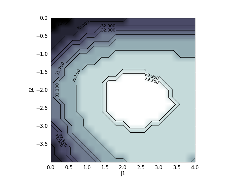
The numerical iteration of this dynamical system is fast. It allows to obtain the theoretical performance that can be achieved in an infinite- system. We have used it in particular to estimate the values of that have good performance. For Gauss-Bernoulli signals, using optimal choices of , we have found that perfect reconstruction can be obtained down to the theoretical limit by taking (with correction that scale as ). Recent rigorous work by Donoho, Javanmard and Montanari Donoho et al. (2011) extends our work and proves our claim that s-BP can reach the optimal threshold asymptotically.
Practical numerical implementation of s-BP matches this theoretical performance only when the size of every block is large enough (few hundreds of variables). In practice, for finite size of the signal, if we want to keep the block-size reasonable we are hence limited to values of of several dozens. Hence in practice we do not quite saturate the threshold , but exact reconstruction is possible very close to it, as illustrated in Fig. 2 in the main text, where the values that we used for the coupling parameters are listed in Table 1.
In Fig. 3, we also presented the result of the s-BP reconstruction of the Gaussian signal of density for different values of . We have observed empirically that the result is rather robust to choices of and . In this case, in order to demonstrate that very different choices give seeding matrices which are efficient, we used , and then and for , and for , and for and and for . One sees that a common aspect to all these choices is a large ratio . Empirically, this seems to be important in order to ensure a short convergence time. A more detailed study of convergence time of the dynamical system will be necessary in order to give some more systematic rules for choosing the couplings. This is left for future work.
Even though our theoretical study of the seeded BP was performed on an example of a specific signal distribution, the examples presented in Figs. 1 and 2 show that the performance of the algorithm is robust and also applies to images which are not drawn from that signal distribution.
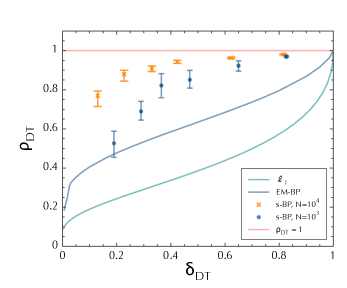
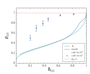
Appendix F Phase diagram in the variables used by Donoho & Tanner (2005)
We show in Fig. 7 the phase diagram in the convention used by Donoho & Tanner (2005), which might be more convenient for some readers.
Appendix G Details on the phantom and Lena examples
In this section, we give a detailed description of the way we have produced the two examples of reconstruction in Fig. 1. It is important to stress that this figure is intended to be an illustration of the s-BP reconstruction algorithm. As such, we have used elementary protocols to produce true -sparse signals and have not tried to optimize the sparsity nor to use the best possible compression algorithm; instead, we have limited ourselves to the simplest Haar wavelet transform, to make the exact reconstruction and the comparison between the different approaches more transparent.
The Shepp-Logan example is a picture that has been generated using the Matlab implementation. The Lena picture is a crop of the gray version of the standard test image. In the first case, we have worked with the sparse one-step Haar transform of the picture, while in the second one, we have worked with a modified picture where we have kept the percent of largest (in absolute value) coefficients of the two-step Haar transform, while putting all others to zero. The datasets of the two images are available online noteASPICS (7). Compressed sensing here is done as follows: The original image is a vector o of pixels. The unknown vector are the projections of the original image on a basis of one- or two-steps Haar wavelets. It is sparse by construction. We generate a matrix F as described above, and construct . The measurements are obtained by , and the linear system for which one does reconstruction is . Once x has been found, the original image is obtained from . We used EM-BP and s-BP with a Gauss-Bernoulli .
On the algorithmic side, the EM-BP and experiments were run with the same full gaussian random measurement matrices. The minimization of the norm was done using the -magic tool for Matlab, which is a free implementation that can be download at http://users.ece.gatech.edu/~justin/l1magic/, using the lowest possible tolerance such that the algorithm outputs a solution. The coupling parameters of s-BP are given in Table 2. A small damping was used in each iterations, we mixed the old and new messages, keeping of the messages from the previous iteration. Moreover, since for both Lena and the phantom, the components of the signal are correlated, we have permuted randomly the columns of the sensing matrix . This allows to avoid the (dangerous) situation where a given block contains only zero signal components.
Note that the number of iterations needed by the s-BP procedure to find the solution is moderate. The s-BP algorithm coded in Matlab finds the image in few seconds. For instance, the Lena picture at requires about iterations and about seconds on a standard laptop. Even for the most difficult case of Lena at , we need around iterations, which took only about minutes. In fact, s-BP (coded in Matlab) is much faster than the Matlab implementation of -magic on the same machine. We report the MSE for all these reconstruction protocols in Table 3.
| BP | |||||
|---|---|---|---|---|---|
| s-BP |
| 0 | |||||
| BP | 0 | ||||
| s-BP |
Appendix H Performance of the algorithm in the presence of measurement noise
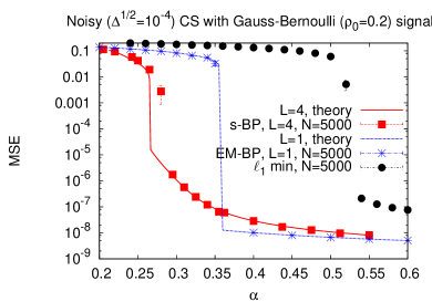
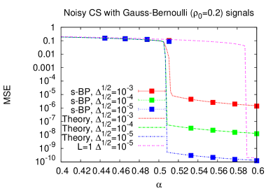
A systematic study of our algorithm for the case of noisy measurements can be performed using the replica analysis, but goes beyond the scope of the present work. In this section we however want to point out two important facts: 1) the modification of our algorithm to take into account the noise is straightforward, 2) the results that we have obtained are robust to the presence of a small amount of noise. As shown in section B, the probability of x after the measurement of y is given by
| (67) |
is the variance of the Gaussian noise in measurement . For simplicity, we consider that the noise is homogeneous, i.e., , for all , and discuss the result in unit of standard deviation . The AMP-form of the message passing including noise have already been given in section C. The variance of the noise, , can also be learned via expectation maximization approach, which reads:
| (68) |
The dynamical system describing the density evolution has been written in Sect. E. It just needs to be complemented by the iteration on according to Eq. (68). We have used it to study the evolution of MSE in the case where both and signal distribution are Gauss-Bernoulli with density , zero mean and unit variance for the full measurement matrix and for the seeding one. Figure 8 shows the MSE as a function of for a given , using our algorithm, and the minimization for comparison. The analytical results obtained by the study of the dynamical system are compared to numerical simulations, and agree very well.
References
- Candès & Wakin 2008 Candès, E. J. & Wakin, M. B. An Introduction To Compressive Sampling. IEEE Signal Processing Magazine 25, 21–30 (2008).
- Duarte et al. 2008 Duarte, M. F., Davenport, M.A., Takhar, D., Laska, J.N., Ting Sun, Kelly, K.F. & Baraniuk, R.G. Single-pixel imaging via compressive sampling. IEEE Signal Processing Magazine 25, 83 (2008).
- Candès & Tao 2005 Candès, E. J. & Tao, T. Decoding by linear programming. IEEE Trans. Inform. Theory 51, 4203 (2005).
- Donoho 2006 Donoho, D. L. Compressed sensing. IEEE Trans. Inform. Theory 52, 1289 (2006).
- Donoho & Tanner 2005 Donoho, D. L. & Tanner, J. Neighborliness of randomly projected simplices in high dimensions. Proc. Natl. Acad. Sci. 102, 9452–9457 (2005).
- Mézard et al. 1987 Mézard, M., Parisi, G. & Virasoro, M. A. Spin-Glass Theory and Beyond, vol. 9 of Lecture Notes in Physics (World Scientific, Singapore, 1987).
- 7 Applying Statistical Physics to Inference in Compressed Sensing http://aspics.krzakala.org
- Wu & Verdu 2011a Wu, Y. & Verdu, S. MMSE Dimension. Information Theory, IEEE Transactions on 57, 4857 –4879 (2011a).
- Wu & Verdu 2011b Wu, Y. & Verdu, S. Optimal Phase Transitions in Compressed Sensing (2011b). ArXiv:1111.6822v1 [cs.IT].
- Guo et al. 2009 Guo, D., Baron, D. & Shamai, S. A single-letter characterization of optimal noisy compressed sensing. In Communication, Control, and Computing, 2009. Allerton 2009. 47th Annual Allerton Conference on, 52 –59 (2009).
- Donoho et al. 2009 Donoho, D. L., Maleki, A. & Montanari, A. Message-passing algorithms for compressed sensing. Proc. Natl. Acad. Sci. 106, 18914–18919 (2009).
- Kabashima et al. 2009 Kabashima, Y., Wadayama, T. & Tanaka, T. A typical reconstruction limit of compressed sensing based on Lp-norm minimization. J. Stat. Mech. L09003 (2009).
- Rangan et al. 2009 Rangan, S., Fletcher, A. & Goyal, V. Asymptotic Analysis of MAP Estimation via the Replica Method and Applications to Compressed Sensing. arXiv:0906.3234v2 (2009).
- Ganguli & Sompolinsky 2010 Ganguli, S. & Sompolinsky, H. Statistical Mechanics of Compressed Sensing. Phys. Rev. Lett. 104, 188701 (2010).
- Pearl 1982 Pearl, J. Reverend Bayes on inference engines: A distributed hierarchical approach. In Proceedings American Association of Artificial Intelligence National Conference on AI, 133–136 (Pittsburgh, PA, USA, 1982).
- Richardson & Urbanke 2008 Richardson, T. & Urbanke, R. Modern Coding Theory (Cambridge University Press, 2008).
- Mézard & Montanari 2009 Mézard, M. & Montanari, A. Information, Physics, and Computation (Oxford Press, Oxford, 2009).
- Jimenez Felstrom & Zigangirov 1999 Jimenez Felstrom, A. & Zigangirov, K. Time-varying periodic convolutional codes with low-density parity-check matrix. Information Theory, IEEE Transactions on 45, 2181 –2191 (1999).
- Kudekar et al. 2010 Kudekar, S., Richardson, T. & Urbanke, R. Threshold saturation via spatial coupling: Why convolutional LDPC ensembles perform so well over the BEC. In Information Theory Proceedings (ISIT),, 684–688 (2010).
- Lentmaier & Fettweis 2010 Lentmaier, M. & Fettweis, G. On the thresholds of generalized LDPC convolutional codes based on protographs. In Information Theory Proceedings (ISIT), 709–713 (2010).
- Hassani et al. 2010 Hassani, S., Macris, N. & Urbanke, R. Coupled graphical models and their thresholds. In Information Theory Workshop (ITW),, 1 – 5 (2010).
- Donoho et al. 2010 Donoho, D., Maleki, A. & Montanari, A. Message passing algorithms for compressed sensing: I. motivation and construction. In Information Theory Workshop (ITW), 2010 IEEE, 1 –5 (2010).
- Rangan 2011 Rangan, S. Generalized Approximate Message Passing for Estimation with Random Linear Mixing. In Information Theory Proceedings (ISIT),, 2168 – 2172 (2011).
- Rangan 2010 Rangan, S. Estimation with random linear mixing, belief propagation and compressed sensing. In Information Sciences and Systems (CISS), 2010 44th Annual Conference on, 1 –6 (2010).
- KudekarPfister 2010 Kudekar, S. & Pfister H. The effect of spatial coupling on compressive sensing. In Communication, Control, and Computing, 2009. Allerton 2009. 48th Annual Allerton Conference on, 347 –353 (2010).
- 26 For proper normalization we regularize the linear constraint to , where can be seen as a variance of noisy measurement, and consider the limit , see Appendix A.
- Natarajan 1995 Natarajan, B. K. Sparse Approximate Solutions to Linear Systems. SIAM J. Comput. 24, 227–234 (1995).
- Thouless et al. 1977 Thouless, D. J., Anderson, P. W. & Palmer, R. G. Solution of ‘Solvable Model of a Spin-Glass’. Phil. Mag. 35, 593–601 (1977).
- Tanaka 2002 Tanaka, T. A statistical-mechanics approach to large-system analysis of CDMA multiuser detectors. IEEE Trans. Infor. Theory 48, 2888–2910 (2002).
- Guo & Wang 2006 Guo, D. & Wang, C.-C. Asymptotic Mean-Square Optimality of Belief Propagation for Sparse Linear Systems. Information Theory Workshop, 2006. ITW ’06 Chengdu. 194–198 (2006).
- Kschischang et al. 2001 Kschischang, F. R., Frey, B. & Loeliger, H.-A. Factor graphs and the sum-product algorithm. IEEE Trans. Inform. Theory 47, 498–519 (2001).
- Yedidia et al. 2003 Yedidia, J., Freeman, W. & Weiss, Y. Understanding Belief Propagation and Its Generalizations. In Exploring Artificial Intelligence in the New Millennium, 239–236 (Morgan Kaufmann, San Francisco, CA, USA, 2003).
- Montanari & Bayati 2011 Montanari, A. & Bayati, M. The dynamics of message passing on dense graphs, with applications to compressed sensing. In Information Theory Proceedings (ISIT),, 764 – 785 (2011).
- Dempster et al. 1977 Dempster, A., Laird, N. & Rubin, D. Maximum Likelihood from Incomplete Data via the EM Algorithm. Journal of the Royal Statistical Society 38, 1 (1977).
- Iba 1999 Iba, Y. The Nishimori line and Bayesian statistics. Journal of Physics A: Mathematical and General 32, 3875 (1999).
- Decelle et al. 2011 Decelle, A., Krzakala, F., Moore, C. & Zdeborová, L. Inference and Phase Transitions in the Detection of Modules in Sparse Networks. Phys. Rev. Lett. 107, 065701 (2011).
- Nishimori 2001 Nishimori, H. Statistical Physics of Spin Glasses and Information Processing (Oxford University Press, Oxford, 2001).
- Guo & Verdú 2005 Guo, D. & Verdú, S. Randomly spread CDMA: Asymptotics via statistical physics. IEEE Trans. Infor. Theory 51, 1983–2010 (2005).
- Donoho et al. 2011 Donoho, D. L., Javanmard, A. & Montanari, A. Information-Theoretically Optimal Compressed Sensing via Spatial Coupling and Approximate Message Passing (2011). ArXiv:1112.0708v1 [cs.IT].