Can noncommutativity affect the whole history of the Universe?

Abstract

We study a classical, noncommutative (NC), Friedmann-Robertson-Walker cosmological model. The spatial sections may have positive, negative or zero constant curvatures. The matter content is a generic perfect fluid. The initial noncommutativity between some canonical variables is rewritten, such that, we end up with commutative variables and a NC parameter. Initially, we derive the scale factor dynamic equations for the general situation, without specifying the perfect fluid or the curvature of the spatial sections. Next, we consider two concrete situations: a radiation perfect fluid and dust. We study all possible scale factor behaviors, for both cases. We compare them with the corresponding commutative cases and one with the other. We obtain, some cases, where the NC model predicts a scale factor expansion which may describe the present expansion of our Universe. Those cases are not present in the corresponding commutative models. Finally, we compare our model with another NC model, where the noncommutativity is between different canonical variables. We show that, in general, it leads to a scale factor behavior that is different from our model.

I Introduction

Almost twenty years ago it was possible to conclude from observational data that the Universe is going through a phase of accelerated expansion expansion . After that, many hypothesis appeared in the literature trying to explain this fascinating feature. The different explanations are divided in two major groups: the ones using general relativity (GR) as the correct theory to explain the gravitational phenomena and the others that do not use it. Among the ones in the first group we may mention the models that consider the Universe uniformly filled with a phantom fluid (the dark energy), which would drive the accelerated expansion of the Universe under an equation of state $p/\rho=\alpha<-1/3$, where $\alpha$ is a constant which defines the fluid, $p$ is the fluid pressure and $\rho$ its density phantom . In this context, the cosmological constant is an important candidate to represent the dark energy, since it acts as a fluid with $p/\rho=-1$ ($\Lambda$CDM model), which is consistent with observational results data1 . However, the theoretical value for the cosmological constant (estimated by the physics of high energy particles) conflicts with observational data by 30 orders of magnitude in the energy scale data2 . Despite of this, the role played by the cosmological constant at the FRW cosmological model has been investigated at the quantum level nivaldo and interesting results have been obtained. The positive cosmological constant can take account of the initial inflationary period and also of a late accelerated expansion phase, with an in-between decelerated expansion phase. Also, the past and future cosmological singularities are removed. Among the explanations to the present accelerated expansion using theories other than GR we may mention the ones which modify the 4-dimensional Einstein-Hilbert action by adding higher order curvature invariants. In the simplest examples in this class, the GR action is modified by the addition of Ricci scalar ($R$) functions. They are the so called f(R) theories f(R) . For a review on different theoretical explanations for the present accelerated expansion see Ref. trodden .

Noncommutative ideas were first introduced, a long time ago, by Snyder snyder ; snyder1 . There, the noncommutativity was imposed between the spacetime coordinates and his main motivation was to eliminate the divergences in quantum field theory. Recently, the interest in those ideas of noncommutativity between spacetime coordinates were renewed due to some important results obtained in superstring, membrane and $M$-theories banks ; connes ; chu ; schomerus ; witten . In the past few years, the role played by noncommutativity in cosmological models has been extensively investigated NCC . In this scenario it was possible to prove that the past and future cosmological singularities are removed due to noncommutativity barbosa1 and that the NC effects are relevant to the entire history of the Universe, for intermediary times nelsonP . The main motivation in order to consider noncommutativity in classical cosmology models is the possibility that some residual noncommutative contribution may have survived in later stages of our Universe. Based on these ideas some researchers have proposed some NC models in classical cosmology in order to explain some intriguing results observed by WMAP. Such as a running spectral index of the scalar fluctuations and an anomalously low quadrupole of CMB angular power spectrum huang ; kim ; liu ; huang1 ; kim1 . Another relevant application of NC ideas in semi-classical and classical cosmology is the attempt to explain the present accelerated expansion of our Universe pedram ; obregon ; gil .

In the present work, we would like to contribute to the investigation on the importance of noncommutativity as a possible mechanism to explain the present expansion of the Universe. In this way, we study the noncommutative version of a classical cosmology model. The model has a Friedmann-Robertson-Walker (FRW) geometry, the matter content is, initially, a generic perfect fluid and the spatial sections may have negative, positive or zero constant curvatures. We work in the Schutz’s variational formalism schutz ; germano1 . The noncommutativity is obtained by imposing deformed Poisson brackets between certain canonical variables. Initially, we derive the scale factor dynamic equations for the general situation, without specifying the perfect fluid or the curvature of the spatial sections. Next, we consider two concrete situations: a radiation perfect fluid and dust. We study all possible scale factor behaviors, for both cases. We compare them with the corresponding commutative cases and one with the other. We obtain, some cases, where the NC model predicts a scale factor expansion which may describe the present expansion of our Universe. Those cases are not present in the corresponding commutative models. The noncommutativity that we are about to propose is not the typical noncommutativity between usual spatial coordinates. We are describing FRW models using the Hamiltonian formalism, therefore their phase spaces are given by the canonical variables and conjugated momenta: $\{a,P_{a},T,P_{T}\}$. Then, the noncommutativity we are about to propose will be between these phase space variables. Since these variables are functions of the time coordinate $t$, this procedure is a generalization of the typical noncommutativity between usual spatial coordinates. The noncommutativity between those types of phase space variables have already been proposed in the literature. At the quantum level in Refs. garcia ; nelsonP ; barbosa1 ; obregon and at the classical level in Refs. pedram ; gil . Another motivation of the present work is investigating if different ways of introducing noncommutativity, in the same cosmological model, modify the predictions of the resulting NC models. In this way we present a detailed comparison with another NC model gil .

In Section II, we introduce the noncommutative model for a generic perfect fluid and derive the coupled system of differential equations for the variables. In Section III, we apply the general formalism for the case of a radiation perfect fluid. We solve the system of differential equations and obtain the scale factor as a function of the time coordinate and few parameters, including the NC parameter $\gamma$. We analyze all possible behavior of the solutions, including a comparison with the solutions for the corresponding commutative model, paying special attention for those representing expansion. In Section IV, we repeat the investigation performed in the previous section, this time for the case of a dust perfect fluid. We, also, compare the scale factor behavior for the case of a dust perfect fluid with the behavior for the case of a radiation perfect fluid. In Section V, we present a detailed comparison with another NC model gil , where the noncommutativity is between different canonical variables. We show that, in general, it leads to a scale factor behavior that is different from our model. Finally, in Section VI, we comment on the most important results of the present paper.

II The noncommutative model for any perfect fluid

The FRW cosmological models are characterized by the scale factor $a(t)$ and have the following line element,

$$ds^{2}=-N^{2}(t)dt^{2}+a^{2}(t)\left(\frac{dr^{2}}{1-kr^{2}}+r^{2}d\Omega^{2}\right)\,,$$ (1)

where $d\Omega^{2}$ is the line element of the two-dimensional sphere with unitary radius, $N(t)$ is the lapse function and $k$ gives the type of constant curvature of the spatial sections. It may assume the values $k=-1,1,0$ and we are using the natural unit system, where $c=G=1$. The matter content of the model is represented by a perfect fluid with four-velocity $U^{\mu}=N(t)\delta^{\mu}_{0}$ in the comoving coordinate system used. The total energy-momentum tensor is given by,

$$T_{\mu\nu}=(\rho+p)U_{\mu}U_{\nu}+pg_{\mu\nu}\,,$$ (2)

where $\rho$ and $p$ are the energy density and pressure of the fluid, respectively. Here, we assume that $p=\alpha\rho$, where $\alpha$ is a constant which defines the perfect fluid.

From the metric (1) and the energy momentum tensor (2), one may write the total Hamiltonian of the present model ($N{\mathcal{H}}$), where ${\mathcal{H}}$ is the superhamiltonian constraint. It is given by germano1 ,

$$N{\mathcal{H}}=-\frac{P_{a}^{2}}{24}-6ka^{2}+a^{1-3\alpha}P_{T},$$ (3)

where $P_{a}$ and $P_{T}$ are the momenta canonically conjugated to $a$ and $T$, the latter being the canonical variable associated to the fluid germano1 . Here, we are working in the conformal gauge, where $N=a$.

In order to introduce the noncommutativity in the model, we start considering, initially, that the total Hamiltonian of the model has the same functional form as (3). But now it is written in terms of noncommutative variables,

$$N_{nc}{\mathcal{H}}_{nc}=-\frac{P_{anc}^{2}}{24}-6ka_{nc}^{2}+a_{nc}^{1-3\alpha}P_{Tnc},$$ (4)

Then, we propose that the noncommutative variables of the model $\{a_{nc},P_{anc},T_{nc},P_{Tnc}\}$ satisfy the following deformed Poisson brackets (PBs):

$$\left\{a_{nc},T_{nc}\right\}=\left\{P_{anc},P_{Tnc}\right\}=0,$$ (5)

$$\left\{a_{nc},P_{anc}\right\}=\left\{T_{nc},P_{Tnc}\right\}=1,$$ (6)

$$\left\{a_{nc},P_{Tnc}\right\}=\left\{T_{nc},P_{anc}\right\}=\gamma,$$ (7)

in which $\gamma$ is the NC parameter. It is important to notice that this is not the only possible deformed PBs one may propose, for the present model.

As mentioned, above, in Ref. gil the authors considered a very similar classical, noncommutative, FRW model coupled to a perfect fluid, in the presence of a cosmological constant. The only differences between our NC model and the NC model in Ref. gil are the choices of deformed PBs and the presence of a cosmological constant in their model. In Section V, we shall make a detailed comparison between both models. In their choice of deformed PBs, they made the two PBs in Eq. (5) different from zero, instead of the two PBs in Eq. (7). This can be better seen in Eq. (V). Therefore, since one of our motivations is investigating possible differences among different deformed PBs choices the only possibility, that does not include any of the PBs in Eq. (5), was to make the two PBs in Eq. (7) different from zero. For simplicity we make them equal to the same NC parameter.

We would like to describe those models in terms of usual commutative variables, which satisfy the usual PBs. Because it is simpler to deal with that kind of variables. Following the literature of noncommutative theories it is possible to achieve that by introducing a set of coordinate transformations from the noncommutative variables to new commutative ones. Those type of transformations were first introduced in Refs. susskind and sometimes are called Bopp shift zachos . Due to our choice of deformed PBs (7), the more general transformations, to first order in $\gamma$, leading from the NC variables to new commutative ones, are given by,

$$a_{nc}\rightarrow a_{c}+\frac{\gamma}{2}T_{c},$$

$$P_{anc}\rightarrow P_{ac}+\frac{\gamma}{2}P_{Tc},$$

$$T_{nc}\rightarrow T_{c}+\frac{\gamma}{2}a_{c},$$ (8)

$$P_{Tnc}\rightarrow P_{Tc}+\frac{\gamma}{2}P_{ac},$$

where the commutative variables have $c$ labels. It is important to notice that if we introduce the noncommutative variables Eq. (II), in the deformed PBs Eq. (5-7) and use the usual PBs among the commutative variables, they are satisfied to first order in $\gamma$. Another important motivation to use those commutative variables, is that, the metric for those models may be written in terms of them as,

$$ds^{2} = -\left(a_{c}(t)+\frac{\gamma}{2}T_{c}(t)\right)^{2}dt^{2}$$ (9)

$$+ \left(a_{c}(t)+\frac{\gamma}{2}T_{c}(t)\right)^{2}\left(\frac{dr^{2}}{1-kr^{2}}+r^{2}d\Omega^{2}\right)\,.$$

For $\gamma=0$, this metric reduces to Eq. (1), in the gauge $N=a$. Observing the metric Eq. (9), we notice that the dynamics of world lines separations between two different times is given by the NC scale factor,

$$a_{nc}(t)=a_{c}(t)+\frac{\gamma}{2}T_{c}(t).$$ (10)

Therefore, in our study of the dynamics of the models described by the metric Eq. (9), we must compute the NC scale factor given by Eq. (10). Since, all quantities in that metric Eq. ($\ref{5,5})$ are commutative, we can treat those models using the usual general relativity methods. In particular, if we write the conservation equation for the fluid stress-energy tensor Eq. (2), for the metric Eq. (9), we obtain the following relationship between the fluid density and the NC scale factor,

$$\rho(t)=\bar{C}\left(a_{c}(t)+\frac{\gamma}{2}T_{c}(t)\right)^{-3(\alpha+1)},$$ (11)

where $\bar{C}$ is a positive constant. In terms of the commutative variables Eq. (II), we have two equivalent ways to write the equations that describe the dynamics of the models. In the first one, we write the Einstein’s equation for the metric Eq. (9), use the expression for $\rho(t)$ Eq. (11) and the equation of state for the fluid. In the second way, we introduce the transformations Eq. (II) in the total Hamiltonian Eq. (4) and compute the Hamilton’s equations for the commutative variables. Since both ways are entirely equivalent, we shall use the second way.

We start rewriting the total Hamiltonian $N_{nc}{\mathcal{H}}_{nc}$ Eq. (4), in terms of the commutative variables Eq. (II),

$$N_{nc}{\mathcal{H}}_{nc} = -\frac{1}{24}\left(P_{ac}+\frac{\gamma}{2}P_{Tc}\right)^{2}-6k\left(a_{c}+\frac{\gamma}{2}T_{c}\right)^{2}$$ (12)

$$+ \left(a_{c}+\frac{\gamma}{2}T_{c}\right)^{1-3\alpha}\left(P_{Tc}+\frac{\gamma}{2}P_{ac}\right),$$

The Hamilton’s equations of motion, obtained using the total Hamiltonian Eq. (12) and the usual PBs among the commutative variables, are,

$$\dot{a}_{c} = \left\{a_{c},N_{nc}{\cal{H}}_{nc}\right\}=-\frac{1}{12}\left(P_{ac}+\frac{\gamma}{2}P_{Tc}\right)$$ (13)

$$+ \frac{\gamma}{2}\left(a_{c}+\frac{\gamma}{2}T_{c}\right)^{1-3\alpha},$$

$$\dot{P}_{ac} = \left\{P_{ac},N_{nc}{\cal{H}}_{nc}\right\}=12k\left(a_{c}+\frac{\gamma}{2}T_{c}\right)$$ (14)

$$- (1-3\alpha)\left(a_{c}+\frac{\gamma}{2}T_{c}\right)^{-3\alpha}\left(P_{Tc}+\frac{\gamma}{2}P_{ac}\right),$$

$$\dot{T}_{c} = \left\{T_{c},N_{nc}{\cal{H}}_{nc}\right\}=-\frac{\gamma}{24}\left(P_{ac}+\frac{\gamma}{2}P_{Tc}\right)$$ (15)

$$+ \left(a_{c}+\frac{\gamma}{2}T_{c}\right)^{1-3\alpha},$$

$$\dot{P}_{Tc} = \left\{P_{Tc},N_{nc}{\cal{H}}_{nc}\right\}=6\gamma k\left(a_{c}+\frac{\gamma}{2}T_{c}\right)$$ (16)

$$- (1-3\alpha)\frac{\gamma}{2}\left(a_{c}+\frac{\gamma}{2}T_{c}\right)^{-3\alpha}\left(P_{Tc}+\frac{\gamma}{2}P_{ac}\right)$$

Now, we would like to find the NC scale factor behavior (10). In the general situation, for generic $\alpha$ and $k$, the best we can do is writing, from Eqs. (13)-(16), a system of two coupled differential equations involving $a_{c}(t)$, $T_{c}(t)$ and their time derivatives. This is done in the following way. Combining Eqs. (14) and (16), we obtain the following relationship between $P_{Tc}$ and $P_{ac}$,

$$P_{Tc}=\frac{\gamma}{2}P_{ac}+C,$$ (17)

where $C$ is an integration constant. Physically, for the commutative case ($\gamma=0$), $C$ represents the fluid energy, which means that it is positive. Then, using Eqs. (13) and (15), we find, to first order in $\gamma$, the following equation expressing $P_{ac}$ in terms of time derivatives of $a_{c}$ and $T_{c}$,

$$P_{ac}=-12\dot{a}_{c}+6\gamma\dot{T}_{c}-\frac{\gamma}{2}C.$$ (18)

Finally, we introduce the values of $\dot{P}_{ac}$ Eq. (14), $\dot{T}_{c}$ Eq. (15), $\dot{P}_{Tc}$ Eq. (16), $P_{Tc}$ Eq. (17) and $P_{ac}$ Eq. (18), in the time derivative of Eq. (13) and in Eq. (15). It gives, to first order in $\gamma$, the following system of coupled differential equation for $a_{c}$ and $T_{c}$,

$$\ddot{a}_{c}(t) = -k\left(a_{c}(t)+\frac{\gamma}{2}T_{c}(t)\right)$$ (19)

$$- (1-3\alpha)\left(\frac{\gamma}{2}\dot{a}_{c}(t)-\frac{C}{12}\right)\left(a_{c}(t)+\frac{\gamma}{2}T_{c}(t)\right)^{-3\alpha}$$

$$\dot{T}_{c}(t) = \frac{\gamma}{2}\dot{a}_{c}(t)+\left(a_{c}(t)+\frac{\gamma}{2}T_{c}(t)\right)^{1-3\alpha}.$$ (20)

All the information about the noncommutativity is encoded in the parameter $\gamma$. If we set it to zero we recover the usual commutative model in the gauge $N=a$. In particular, equation (19) decouples and we may solve it to obtain the scale factor dynamics. In order to solve those equations and compute $a_{nc}$ Eq. (10), we shall have to furnish initial conditions for $a_{c}(t)$, $\dot{a}_{c}(t)$ and $T_{c}(t)$. Unfortunately, we cannot find algebraic solutions for $a_{c}(t)$ and $T_{c}(t)$, from the system Eqs. (19)-(20), for generic values of $\alpha$ and $\gamma$. On the other hand, we may solve them for certain types of perfect fluids. Therefore, in what follows, we shall investigate two important cases, where we can find algebraic solutions for $a_{c}(t)$ and $T_{c}(t)$, the radiation perfect fluid and the dust perfect fluid.

III The noncommutative model for a radiation perfect fluid

Let us consider, initially, the case of a radiation perfect fluid. Therefore, we assume that $p=\rho/3$, which is the equation of state for radiation. This choice may be considered as a first approximation to treat the matter content of the early Universe and it was made as a matter of simplicity. It is clear that a more complete treatment should describe the radiation, present in the primordial Universe, in terms of the electromagnetic field.

If we introduce $\alpha=1/3$ in Eq. (20), we may integrate the resulting equation, in the $t$ variable, to obtain $T_{c}$ as the following function of $a_{c}$.

$$T_{c}(t)=\frac{\gamma}{2}(a_{c}(t)-a_{0})+t+T_{0}.$$ (21)

Where $a_{0}$ and $T_{0}$ are, respectively, the initial values ($t=0$) of $a_{c}(t)$ and $T_{c}(t)$. If we introduce $\alpha=1/3$ and the value of $T(t)$ Eq. (21), in Eq. (19), we obtain, to first order in $\gamma$, the following differential equation for $a_{c}(t)$,

$$\ddot{a}_{c}(t)+ka_{c}(t)+\frac{\gamma}{2}k(t+T_{0})=0,$$ (22)

If we set $\gamma=0$, in Eq. (22), the commutative FRW cosmological model is restored. In what follows, we will solve Eq.(22), analytically, for $k=0,\pm 1$. Then, we will compute the NC scale factor Eq. (10), with the aid of $a_{c}(t)$ Eq. (22) and $T_{c}(t)$ Eq. (21). Finally, we will explore some features of those solutions, for several values of $\gamma$.

III.1 The case $k=0$

For spacetimes with flat spatial sections, $k=0$, Eq. (22), reduces to the commutative case. If we solve this equation, we obtain the following scale factor expression,

$$a_{c}(t)=v_{0}t+a_{0},$$ (23)

where $v_{0}$ is the initial value ($t=0$) of $\dot{a}_{c}(t)$. This is exactly the scale factor in the usual commutative model, which we will write $a_{c,\gamma=0}(t)$. As mentioned, above, the NC scale factor Eq. (10) is the physical one associated with the metric Eq. (9). In order to compute it, we start evaluating $T_{c}(t)$ Eq. (21), with the aid of $a_{c}(t)$ Eq. (23). Finally, we obtain the NC scale factor Eq. (10), to first order in $\gamma$, with the aid of $T_{c}(t)$ and $a_{c}(t)$ Eq. (23),

$$a_{nc}(t)=\left(v_{0}+\frac{\gamma}{2}\right)t+a_{0}+T_{0}.$$ (24)

In order to compare the NC scale factor Eq. (24) with the usual commutative one $a_{c,\gamma=0}(t)$, which in this case is given by Eq. (23), let us set $T_{0}=0$ in Eq. (24). It is done in order to assure that both of them have the same initial value $a_{0}$. Then, we notice that both scale factors are linear functions of $t$, with the same $a$-intercept and different slopes. For $v_{0}>0$, if $\gamma>0$, the NC scale factor increases more rapidly than $a_{c,\gamma=0}(t)$ Eq. (23). On the other hand, if $\gamma<0$ and $v_{0}>|\gamma/2|$, the NC scale factor increases slower than $a_{c,\gamma=0}(t)$. Finally, if $\gamma<0$ and $v_{0}<|\gamma/2|$, the NC scale factor decreases from $a_{0}$ until the Big Crunch.

III.2 The case $k=1$

For spacetimes with constant positive spatial sections, $k=1$, Eq. (22), describes a driven harmonic oscillator, under the driving force $-(\gamma/2)(t+T_{0})$. If we solve this equation, we obtain the following scale factor expression,

$$a_{c}(t)=\left(v_{0}+\frac{\gamma}{2}\right)\sin(t)+\left(a_{0}+\frac{\gamma}{2}T_{0}\right)\cos(t)-\frac{\gamma}{2}(t+T_{0}).$$ (25)

Now, in order to compute the NC scale factor Eq. (10), we start evaluating $T_{c}(t)$ Eq. (21). With the aid of $a_{c}(t)$ Eq. (25), it is given, to first order in $\gamma$, by,

$$T_{c}(t)=\frac{\gamma}{2}\left(v_{0}\sin(t)+a_{0}\cos(t)-a_{0}\right)+t+T_{0}.$$ (26)

Finally, using $a_{c}(t)$ Eq. (25) and $T_{c}(t)$ Eq. (26), the NC scale factor Eq. (10) is given, to first order in $\gamma$, by,

$$a_{nc}(t)=\left(v_{0}+\frac{\gamma}{2}\right)\sin(t)+\left(a_{0}+\frac{\gamma}{2}T_{0}\right)\cos(t).$$ (27)

Now, we would like to compare the NC scale factor Eq. (27) with the usual commutative one $a_{c,\gamma=0}(t)$. We shall set $T_{0}=0$ in $a(t)$ Eq. (27). In order to obtain $a_{c,\gamma=0}(t)$, we set $\gamma=0$ in Eqs. (25) or (27). It gives,

$$a_{c,\gamma=0}(t)=v_{0}\sin(t)+a_{0}\cos(t).$$ (28)

The commutative solution Eq. (28) describes an universe that starts expanding from $a_{0}$ at $t=0$, expands to a maximum size and then contracts back to a Big Crunch singularity, in a finite time. On the other hand, the NC solution Eq. (27), may describe different scale factor behaviors. We studied that solution for several different values of $\gamma$ and reached the following conclusions, for any values of $a_{0}$ and $v_{0}$. For positive $\gamma$, the NC solutions have the same general behavior than the commutative solution, except that their maximum sizes are bigger than the commutative one and they take greater times, than the commutative one, to return to $a=0$. If we increase the absolute value of $\gamma$, that behavior becomes even more pronounced. Therefore, we conclude that when $\gamma$ is positive, the resulting effect upon the scale factor dynamics is the appearance of an additional repulsive force, compared to the commutative case. An example of this case is shown in Figure 1. For negative $\gamma$, the NC solutions have the same general behavior than the commutative solution. The differences are that their maximum sizes are smaller than the commutative one and they take shorter times, than the commutative solution, to return to $a=0$. If we increase the absolute values of $\gamma$, that behavior becomes even more pronounced. Therefore, we conclude that when $\gamma$ is negative, the resulting effect upon the scale factor dynamics is the appearance of an additional attractive force, compared to the commutative case. An example of this case is shown in Figure 2.

Figure 1: Scale factor behavior for both commutative and noncommutative cases, when $k=1$. Here, we consider $\gamma=0.5$, $a_{0}=1$ and $v_{0}=1$. The $a(t)$ for the noncommutative case is the upper curve.

Figure 2: Scale factor behavior for both commutative and noncommutative cases, when $k=1$. Here, we consider $\gamma=-0.5$, $a_{0}=1$ and $v_{0}=1$. The $a(t)$ for the commutative case is the upper curve.

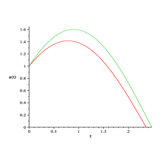
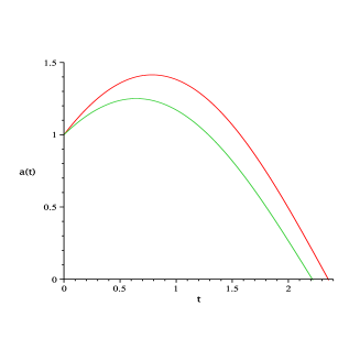
III.3 The case $k=-1$

Solving Eq. (22) for spacetimes with constant negative spatial sections, $k=-1$, we obtain the following scale factor expression,

$$a_{c}(t)=\left(v_{0}+\frac{\gamma}{2}\right)\sinh(t)+\left(a_{0}+\frac{\gamma}{2}T_{0}\right)\cosh(t)-\frac{\gamma}{2}(t+T_{0}).$$ (29)

Now, in order to compute the NC scale factor Eq. (10), we start evaluating $T_{c}(t)$ Eq. (21). With the aid of $a_{c}(t)$ Eq. (29), it is given, to first order in $\gamma$, by,

$$T_{c}(t)=\frac{\gamma}{2}\left(v_{0}\sinh(t)+a_{0}\cosh(t)-a_{0}\right)+t+T_{0}.$$ (30)

Finally, using $a_{c}(t)$ Eq. (29) and $T_{c}(t)$ Eq. (30), the NC scale factor Eq. (10) is given, to first order in $\gamma$, by,

$$a_{nc}(t)=\left(v_{0}+\frac{\gamma}{2}\right)\sinh(t)+\left(a_{0}+\frac{\gamma}{2}T_{0}\right)\cosh(t).$$ (31)

Now, we would like to compare the NC scale factor Eq. (31) with the usual commutative one $a_{c,\gamma=0}(t)$. We shall set $T_{0}=0$ in $a(t)$ Eq. (31). In order to obtain $a_{c,\gamma=0}(t)$, we set $\gamma=0$ in Eqs. (29) or (31).

$$a_{c,\gamma=0}(t)=v_{0}\sinh(t)+a_{0}\cosh(t).$$ (32)

The commutative solution Eq. (32) describes an universe that starts from $a_{0}$ at $t=0$ and expands exponentially to an infinity size when the time goes to infinity. On the other hand, the noncommutative solution Eq. (31), may describe different scale factor behaviors. We studied that solution for several different values of $\gamma$ and reached the following conclusions, for any value of $a_{0}$. For positive $\gamma$ and any value of $v_{0}$, the noncommutative solutions have the same general behavior than the commutative solution, except that they expand in a faster rate than that solution. If we increase the absolute values of $\gamma$, that behavior becomes even more pronounced. Therefore, we conclude that when $\gamma$ is positive, the resulting effect upon the scale factor dynamics is the appearance of an additional repulsive force, compared to the commutative case. An example of this case is shown in Figure 3. For negative $\gamma$ and $v_{0}>|\gamma/2|$, the NC scale factor has the same general behavior than the commutative solution, except that it expands in a slower rate than that solution. An example of this case is shown in Figure 4. For negative $\gamma$ and $v_{0}<|\gamma/2|$, the NC scale factor starts contracting from $a_{0}$ until it reaches a minimum value. Then, it expands exponentially to infinity in a slower rate than the commutative solution. An example of this case is shown in Figure 5. If we increase the absolute values of $\gamma$, that behavior becomes even more pronounced. Therefore, we conclude that when $\gamma$ is negative, the resulting effect upon the scale factor dynamics is the appearance of an additional attractive force, compared to the commutative case.

Figure 3: Scale factor behavior for both commutative and noncommutative cases, when $k=-1$. Here, we consider $\gamma=0.5$, $a_{0}=1$ and $v_{0}=1$. The $a(t)$ for the noncommutative case is the upper curve.

Figure 4: Scale factor behavior for both commutative and noncommutative cases, when $k=-1$. Here, we consider $\gamma=-0.5$, $a_{0}=1$ and $v_{0}=1$. The $a(t)$ for the commutative case is the upper curve.

Figure 5: Scale factor behavior for both commutative and noncommutative cases, when $k=-1$. Here, we consider $\gamma=-0.5$, $a_{0}=1$ and $v_{0}=0$. The $a(t)$ for the commutative case is the upper curve.

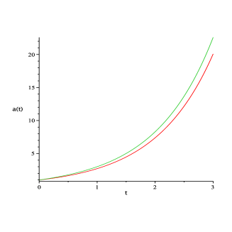
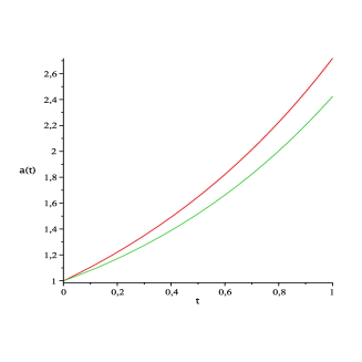
IV The noncommutative model for a dust perfect fluid

Let us consider, now, the case of a dust perfect fluid. Therefore, we assume that $p=0$, which is the equation of state for dust. This choice may be considered as a first approximation to treat the matter content of the present Universe which is dominated by matter that interacts weakly.

If we introduce $\alpha=0$ in Eqs. (19)-(20), we obtain the new system of equations for $a_{c}$ and $T_{c}$,

$$\ddot{a}_{c}(t) = -k\left(a_{c}(t)+\frac{\gamma}{2}T_{c}(t)\right)-\frac{\gamma}{2}\dot{a}_{c}(t)+\frac{C}{12},$$ (33)

$$\dot{T}_{c}(t) = \frac{\gamma}{2}\dot{a}_{c}(t)+a_{c}(t)+\frac{\gamma}{2}T_{c}(t).$$ (34)

Here, also, if we set $\gamma=0$ the commutative FRW cosmological model is restored. In what follows, we will solve the system Eqs. (33)-(34) to find $a_{c}(t)$ and $T_{c}(t)$. Subsequently, we shall combine those solutions to compute the NC scale factor Eq. (10). Finally, we shall explore some features of $a_{nc}(t)$, for several values of $\gamma$, $C$ and $k=0,\pm 1$. We shall, also, compare the present results with the ones of Section III, for a radiation perfect fluid.

IV.1 The case $k=0$

Setting $k=0$ in Eq. (33), we obtain,

$$\ddot{a}_{c}(t)=-\frac{\gamma}{2}\dot{a}_{c}(t)+\frac{C}{12}.$$ (35)

This equation describes the scale factor dynamics under the action of two forces: a positive constant one and a velocity dependent one. For $\gamma=0$, we obtain, from Eq. (35), the scale factor equation for the commutative case. The solution to that equation is given by,

$$a_{c,\gamma=0}(t)=\frac{1}{24}Ct^{2}+v_{0}t+a_{0}.$$ (36)

Now, integrating Eq. (35), we obtain the following expression for $a_{c}(t)$,

$$a_{c}(t)=-\frac{e^{-\gamma t/2}(6\gamma v_{0}-C)}{3\gamma^{2}}+\frac{Ct}{6\gamma}+\frac{3\gamma^{2}a_{0}+6\gamma v_{0}-C}{3\gamma^{2}}.$$ (37)

If we take the limit $\gamma\to 0$ of $a_{c}(t)$ Eq. (37), we obtain the commutative solution $a_{c,\gamma=0}(t)$ Eq. (36). Now, in order to compute the NC scale factor Eq. (10), we must start solving equation (34) in order to find $T_{c}(t)$. With the aid of $a_{c}(t)$ Eq. (37), it is given, to first order in $\gamma$, by,

$$T_{c}(t) =\exp(\gamma t/2)\left(T_{0}+\frac{2a_{0}}{\gamma}\right)$$ (38)

$$+ \left(v_{0}+\frac{2C}{3\gamma^{3}}\right)\sinh(\gamma t/2)+\left(\frac{C}{6\gamma}+\frac{4v_{0}}{\gamma^{2}}\right)\cosh(\gamma t/2)$$

$$- \frac{2a_{0}}{\gamma}-\frac{C}{6\gamma}-\frac{4v_{0}}{\gamma^{2}}-\frac{Ct}{3\gamma^{3}}.$$

Finally, using $a_{c}(t)$ Eq. (37) and $T_{c}(t)$ Eq. (38), the NC scale factor Eq. (10) is given, to first order in $\gamma$, by,

$$a_{nc}(t) =\frac{v_{0}}{2\gamma}(4+\gamma^{2})\sinh(\gamma t/2)$$ (39)

$$+ \frac{C}{12\gamma^{2}}(4+\gamma^{2})\cosh(\gamma t/2)-\frac{C}{12\gamma^{2}}(4+\gamma^{2})$$

$$+ \frac{1}{2}(\gamma T_{0}+2a_{0})\exp(\gamma t/2).$$

Now, we would like to compare the NC scale factor Eq. (39) with the usual commutative one $a_{c,\gamma=0}(t)$ Eq. (36). We shall set $T_{0}=0$ in $a_{nc}(t)$ Eq. (39).

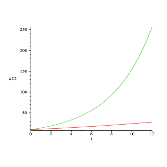
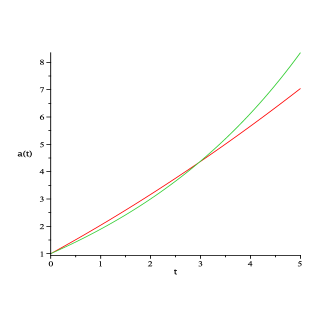
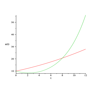
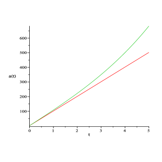
The commutative solution Eq. (36) describes an universe that starts from $a_{0}$ at $t=0$ and expands, as a second degree polynomial in $t$, to an infinity size when $t$ goes to infinity. On the other hand, the noncommutative solution Eq. (39), may describe different scale factor behaviors. We studied that solution for several different values of $\gamma$ and $C$ and reached the following conclusions. For positive $\gamma$, the noncommutative solutions have the same general behavior than the commutative solution, except that they expand in a faster rate than the commutative one. In fact, it expands as an exponential function of $t$. If we increase $\gamma$, that behavior becomes even more pronounced. If we increase $C$, both commutative and noncommutative solutions increase their expansion rates, but the noncommutative solutions still expand faster than the commutative one. Those results are valid for any values of $a_{0}$ and $v_{0}$. An example of this case is shown in Figure 6. For negative $\gamma$, the noncommutative solutions have the same general behavior than the commutative solution, except that they initially expand in a slower rate than the commutative one. Then, they increase their expansion rate and eventually overtake the commutative solution. From that moment onward the noncommutative solutions expand in a faster rate than the commutative one. An example of this case is shown in Figure 7. For sufficiently large values of $a_{0}$ the noncommutative solutions, initially, decrease until reach a minimum value. Then, they start increasing until overtake the commutative solution. An example of this case is shown in Figure 8. For sufficiently large values of $v_{0}$ the noncommutative solutions always expand faster than the commutative one. An example of this case is shown in Figure 9. If we increase the modulus of $\gamma$, those behaviors becomes even more pronounced. If we increase $C$, both commutative and noncommutative solutions increase their expansion rates, but the previous behaviors still take place. From Eq. (39), we can see that for sufficiently large values of $t$, the NC scale factor has an exponential expansion. Since, the dust perfect fluid represents the present matter dominated era of our Universe and $k=0$ is a good candidate to describe its spatial curvature, then, under those circumstances, our NC model may be considered a possible candidate to describe the present expansion of the Universe.

Figure 6: Scale factor behavior for both commutative and noncommutative cases, when $k=0$. Here, we consider $\gamma=0.5$, $C=1$ $a_{0}=10$ and $v_{0}=1$. The $a(t)$ for the noncommutative case is the upper curve.

Figure 7: Scale factor behavior for both commutative and noncommutative cases, when $k=0$. Here, we consider $\gamma=-0.5$, $C=1$ $a_{0}=1$ and $v_{0}=1$. The $a(t)$ for the noncommutative case is the one that expands asymptotically in a faster rate.

Figure 8: Scale factor behavior for both commutative and noncommutative cases, when $k=0$. Here, we consider $\gamma=-0.5$, $C=1$ $a_{0}=10$ and $v_{0}=1$. The $a(t)$ for the commutative case is the one that is strictly increasing.

Figure 9: Scale factor behavior for both commutative and noncommutative cases, when $k=0$. Here, we consider $\gamma=-0.5$, $C=1$ $a_{0}=1$ and $v_{0}=100$. The $a(t)$ for the noncommutative case is the upper curve.

IV.2 The case $k=1$

If we set $k=1$ in the system Eqs. (33)-(34), we may integrate it to find the following algebraic solutions for $a_{c}(t)$,

$$a_{c}(t) = \left(a_{0}+\frac{\gamma}{2}(v_{0}+T_{0})-\frac{C}{12}\right)\cos(t)$$

$$+ \left(v_{0}+\frac{\gamma C}{24}\right)\sin(t)-\frac{\gamma}{2}\left(\frac{C}{12}t+v_{0}+T_{0}\right)+\frac{C}{12},$$

and $T_{c}(t)$,

$$T_{c}(t) = \left(a_{0}+\frac{\gamma}{2}(v_{0}+T_{0})-\frac{C}{12}\right)\sin(t)$$

$$- \left(v_{0}+\frac{\gamma C}{24}\right)\cos(t)+\frac{C}{12}t+v_{0}+T_{0}+\frac{\gamma C}{24}.$$

Now, we can compute $a_{nc}$ Eq. (10), with the aid of $a_{c}(t)$ Eq. (IV.2) and $T_{c}(t)$ Eq. (IV.2). It is given, to first order in $\gamma$, by,

$$a_{nc}(t) = \left(a_{0}+\frac{\gamma}{2}T_{0}-\frac{C}{12}\right)\cos(t)$$ (42)

$$+ \left(v_{0}+\frac{\gamma}{2}a_{0}\right)\sin(t)+\frac{C}{12}.$$

If we set $\gamma=0$ in Eqs. (IV.2) or (42), we obtain the scale factor in the usual commutative model,

$$a_{c,\gamma=0}(t)=\left(a_{0}-\frac{C}{12}\right)\cos(t)+v_{0}\sin(t)+\frac{C}{12}.$$ (43)

Now, we would like to compare the NC scale factor Eq. (42) with the usual commutative one $a_{c,\gamma=0}(t)$ Eq. (43). We shall set $T_{0}=0$ in $a_{nc}(t)$ Eq. (42).

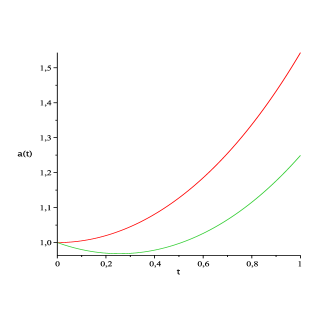
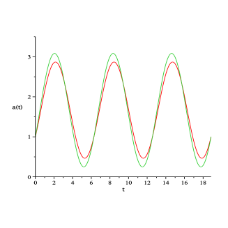
The commutative solution Eq. (43) describes an universe that starts expanding from $a_{0}$ at $t=0$, expands to a maximum size and then contracts. For small values of $C$ it will contract to a Big Crunch singularity. If we increase the value of $C$, both the maximum size and the time interval between $a_{0}$ and the Big Crunch increase. This behavior is similar to the radiation case Subsection III.2. For sufficiently large values of $C$ the scale factor will contract to a minimum value, greater than zero, and then it will expand again. It will continue to oscillate, for ever, between maxima and minima values. If we increase the value of $C$, both maxima and minima values will increase. The minima values will increase until they reach the value $a_{0}$. On the other hand, the noncommutative solution Eq. (42), may describe different scale factor behaviors. We studied that solution for several different values of $\gamma$ and $C$ and reached the following conclusions. For positive values of $\gamma$ and small values of $C$, the NC solutions have the same general behavior than the commutative solution, except that their maximum sizes are bigger than the commutative one and they take greater times, than the commutative one, to reach the Big Crunch singularity. This behavior is qualitatively very similar to the one described by Eq. (27), for $\gamma>0$, in comparison with the commutative solution Eq. (28), for the radiation model Subsection III.2. An example to this case will produce a figure, qualitatively, very similar to Figure 1. If we increase the values of $C$, for different values of $\gamma>0$, the NC scale factors Eq. (42) still have maxima values greater than the commutative solution but now they reach the Big Crunch singularity first than the commutative solution. Finally, for sufficiently large values of $C$ and different values of $\gamma>0$, the NC scale factors Eq. (42) still have maxima values greater than the ones in the commutative case but now they will contract to minima values, greater than zero and smaller than in the commutative case, and then they will expand again. They will continue to oscillate, for ever, between maxima and minima values. If we increase the value of $C$, both maxima and minima values will increase. The minima values will increase until they reach the value $a_{0}$. The maxima and minima values of $a_{nc}$ Eq. (42) will always be greater and smaller, respectively, than in the commutative solution Eq. (43). The NC and commutative curves cross at $t=n\pi$, where $n=1,2,..$. An example of this cases is shown in Figure 10.

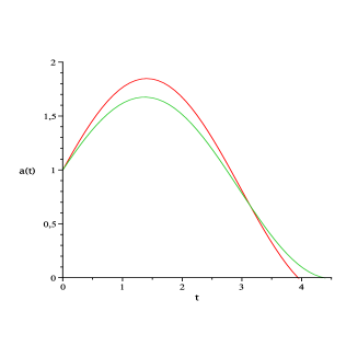
For negative $\gamma$, we found several differences with respect to the cases where $\gamma>0$. For small $C$, the $a_{nc}$ Eq. (42) has a maximum smaller than the commutative one and reach the Big Crunch singularity before the commutative one. This behavior is qualitatively very similar to the one described by Eq. (27), for $\gamma<0$, in comparison with the commutative solution Eq. (28), for the radiation model Subsection III.2. An example to this case will produce a figure, qualitatively, very similar to Figure 2. If we increase the values of $C$, the $a_{nc}$ still have maxima values smaller than the commutative solution but now they reach the Big Crunch singularity after the commutative solution. An example of this case is shown in Figure 11. For sufficiently large values of $C$, $a_{nc}$ will also oscillate, for ever, between maxima and minima values. The difference with respect to the case where $\gamma>0$ is that, here, the maxima and minima values of $a_{nc}$ will always be smaller and greater, respectively, than in the commutative solution. Here, also, the NC and commutative curves cross at $t=n\pi$, where $n=1,2,..$.

The results described above will be valid for any values of $a_{0}$. The different values of $C$, in each domain of that constant, described above, will depend on the value of $v_{0}$. The greater $v_{0}$ the greater is the value of $C$ in each domain.

Figure 10: Scale factor behavior for both commutative and noncommutative cases, when $k=1$. Here, we consider $\gamma=0.5$, $C=20$ $a_{0}=1$ and $v_{0}=1$. The $a(t)$ for the commutative case is the one that has smaller maxima and greater minima.

Figure 11: Scale factor behavior for both commutative and noncommutative cases, when $k=1$. Here, we consider $\gamma=-0.35$, $C=10$ $a_{0}=1$ and $v_{0}=1$. The $a(t)$ for the commutative case is the one that reach $a=0$ first.

IV.3 The case $k=-1$

If we set $k=-1$ in the system Eqs. (33)-(34), we may integrate it to find the following algebraic solutions for $a_{c}(t)$,

$$a_{c}(t) = \left(a_{0}+\frac{\gamma}{2}(-v_{0}+T_{0})+\frac{C}{12}\right)\cosh(t)$$

$$+ \left(v_{0}-\frac{\gamma C}{24}\right)\sinh(t)+\frac{\gamma}{2}\left(\frac{C}{12}t+v_{0}-T_{0}\right)-\frac{C}{12},$$

and $T_{c}(t)$,

$$T_{c}(t) = \left(a_{0}+\frac{\gamma}{2}(v_{0}+T_{0})+\frac{C}{12}\right)\sinh(t)$$ (45)

$$+ \left(v_{0}+\gamma\left(\frac{C}{24}+a_{0}\right)\right)\cosh(t)$$

$$+ \gamma\left(\frac{C}{24}-a_{0}\right)-\frac{C}{12}t-v_{0}+T_{0}.$$

Now, we can compute $a_{nc}$ Eq. (10), with the aid of $a_{c}(t)$ Eq. (IV.3) and $T_{c}(t)$ Eq. (45). It is given, to first order in $\gamma$, by,

$$a_{nc}(t) = \left(a_{0}+\frac{\gamma}{2}T_{0}+\frac{C}{12}\right)\cosh(t)$$ (46)

$$+ \left(v_{0}+\frac{\gamma}{2}a_{0}\right)\sinh(t)-\frac{C}{12}.$$

If we set $\gamma=0$ in Eqs. (IV.3) or (46), we obtain the scale factor in the usual commutative model,

$$a_{c,\gamma=0}(t)=\left(a_{0}+\frac{C}{12}\right)\cosh(t)+v_{0}\sinh(t)-\frac{C}{12}.$$ (47)

Now, we would like to compare the NC scale factor Eq. (46) with the usual commutative one $a_{c,\gamma=0}(t)$ Eq. (47). We shall set $T_{0}=0$ in $a_{nc}(t)$ Eq. (46).

The commutative solution Eq. (47) describes a universe that starts from $a_{0}$ at $t=0$ and expands exponentially to an infinity size when the time goes to infinity. Which is the same behavior described by the commutative solution of the radiation model Eq. (32), Subsection III.3. On the other hand, the noncommutative solution Eq. (46), may describe different scale factor behaviors. We studied that solution for several different values of $\gamma$ and $C$ and reached the following conclusions. For positive $\gamma$, the noncommutative solutions have the same general behavior than the commutative solution, except that they expand in a faster rate than that solution. If we increase the absolute values of $\gamma$, that behavior becomes even more pronounced. Therefore, we conclude that when $\gamma$ is positive, the resulting effect upon the scale factor dynamics is the appearance of an additional repulsive force, compared to the commutative case. An example to this case will produce a figure, qualitatively, very similar to Figure 3. For negative $\gamma$ and $v_{0}>|\gamma/2|a_{0}$, the NC scale factor has the same general behavior than the commutative solution, except that it expands in a slower rate than that solution. An example to this case will produce a figure, qualitatively, very similar to Figure 4. For negative $\gamma$ and $v_{0}<|\gamma/2|a_{0}$, the NC scale factor starts contracting from $a_{0}$ until it reaches a minimum value. Then, it expands exponentially to infinity in a slower rate than the commutative solution. An example to this case will produce a figure, qualitatively, very similar to Figure 5. If we increase the absolute values of $\gamma$ and $a_{0}$, that behavior becomes even more pronounced. Therefore, we conclude that when $\gamma$ is negative, the resulting effect upon the scale factor dynamics is the appearance of an additional attractive force, compared to the commutative case. If we increase the value of $C$ both commutative and noncommutative solutions will expand in a faster rate. But all other properties of those solutions, described above, will remain the same.

V Comparison with a model which has a different choice of deformed Poisson brackets

As mentioned, above, in Ref. gil the authors considered a very similar classical, noncommutative, FRW model coupled to a perfect fluid, in the presence of a cosmological constant. The only differences between the present NC model and the one in Ref. gil are the choices of deformed PBs and the presence of a cosmological constant in their model. Therefore, in this section, we shall compare both models and verify if they lead to the same results or not.

In Ref. gil , the authors introduced the noncommutativity, in the model, using a NC generalized symplectic formalism. As we shall see, this procedure is equivalent to perform transformations, like Eqs. (II), leading from the NC variables to the commutative ones plus a NC parameter. The starting point of both NC models is considering that the total Hamiltonian has the same functional form as Eq. (3). Therefore, initially, it will have the same expression as the total Hamiltonian Eq. (4). In order to be able to compare both NC models, we shall simplify the model introduced in Ref. gil by setting the cosmological constant to zero. In Ref. gil , the noncommutativity is introduced by the following choice of deformed Poisson brackets,

$$\left\{a_{nc},T_{nc}\right\}=\theta,\,\left\{P_{anc},P_{Tnc}\right\}=\beta,$$

$$\left\{a_{nc},P_{anc}\right\}=\left\{T_{nc},P_{Tnc}\right\}=1,$$

$$\left\{a_{nc},P_{Tnc}\right\}=\left\{T_{nc},P_{anc}\right\}=0,$$ (48)

which may be compared to our choice given in Eq. (5). In fact, although the authors of Ref. gil develop the NC generalized symplectic formalism for both deformed PBs introduced in Eq. (V), when they write the resulting total Hamiltonian with the commuting variables plus the NC parameters, they set $\theta=0$. Therefore, we shall restrict our attention to the NC model described by the deformed PBs Eq. (V), with $\theta=0$. In order to describe this model in terms of usual commutative variables, which satisfy the usual PBs, we introduce the following transformations from NC variables to commutative ones,

$$P_{anc} \rightarrow P_{ac}+\beta T_{c},$$

$$a_{nc} \rightarrow a_{c},\,T_{nc}\rightarrow T_{c},\,P_{Tnc}\rightarrow P_{Tc}.$$ (49)

If one introduces the NC variables Eq. (V), in the deformed PBs Eq. (V), with $\theta=0$, and uses the usual PBs among the commutative variables, it is not difficult to show that they are satisfied to first order in $\beta$. Observing the transformations Eqs. (V), we notice the first difference between both models. Here, the $a_{nc}$ coincides with $a_{c}$, therefore the dynamics of the models is described by $a_{c}$. On the other hand, we saw that in our model the dynamics is described by $a_{nc}$ Eq. (10), which does not coincide with $a_{c}$. Now, we rewrite the total Hamiltonian $N_{nc}{\mathcal{H}}_{nc}$ (4), in terms of the commutative variables Eq. (V),

$$N_{nc}{\mathcal{H}}_{nc}=-\frac{(P_{ac}+\beta T_{c})^{2}}{24}-6ka_{c}^{2}+a_{c}^{1-3\alpha}P_{Tc}.$$ (50)

In order to better compare both NC models, we decided to write the model of Ref. gil in the gauge ($N_{nc}=a_{nc}$). It was written originally in the gauge $N=1$. Apart from this difference and few numerical values, the total Hamiltonian (50) coincides with the one obtained in Ref. gil . Now, we would like to compute the scale factor dynamical behavior, for the present NC model. Initially, we compute the Hamilton’s equations from $N_{nc}{\mathcal{H}}_{nc}$ Eq. (50) and, then, combine them to obtain the following second order differential equation, to first order in $\beta$,

$$\ddot{a}_{c}(t) + ka_{c}(t)-\frac{C}{12}(1-3\alpha)a_{c}^{-3\alpha}(t)$$ (51)

$$+ \frac{\beta}{12}(2-3\alpha)a_{c}^{-3\alpha+1}(t)=0,$$

where $C$ has the same physical meaning as in our NC model. Another difference, between both NC models, is that it is possible to write a Friedmann equation, which depends only on $a_{c}(t)$ and its first time derivative, for the present NC model. We shall not write it, here, because it is not possible to do it for our NC model. Equation (51), is the equivalent, in the present NC model, to the system of coupled differential equations (19)-(20), in our NC model. If we set $\gamma=0$, in the system (19)-(20), they decouple and Eq. (19) gives the correct commutative second order differential equation to $a_{c}(t)$. Which is the same equation one obtains, by setting $\beta=0$, in Eq. (51). Observing Eq. (51), we notice another difference between the two NC models. Here, it is possible to write a unique second order differential equation for the scale factor, for a general type of perfect fluid. On the other hand, in our NC model it was not possible. There, we have the system of two coupled differential equations (19)-(20). Since we cannot find algebraic solutions, for a generic perfect fluid, for either the system Eqs. (19)-(20) or the equation (51), we shall restrict our comparisons, between the two NC models, for the radiation and dust perfect fluids. All comparisons between both NC models are done using the same values of $\beta$ and $\gamma$ and the other corresponding parameters in each model.

V.1 Radiation perfect fluid

Setting $\alpha=1/3$ in Eq. (51), we obtain,

$$\ddot{a}_{c}(t)+ka_{c}(t)+\frac{\beta}{12}=0.$$ (52)

This equation must be compared to Eq. (22). The solutions to Eq. (52), for different values of $k$, are given by,

$$a_{c}(t) = -\frac{1}{24}\beta t^{2}+v_{0}t+a_{0},\quad k=0,$$ (53)

$$a_{c}(t) = v_{0}\sin(t)+\left(a_{0}+\frac{\beta}{12}\right)\cos(t)-\frac{\beta}{12},$$ (54)

$$k=1,$$

$$a_{c}(t) = v_{0}\sinh(t)+\left(a_{0}-\frac{\beta}{12}\right)\cosh(t)+\frac{\beta}{12},$$ (55)

$$k=-1.$$

The first important difference between the scale factor behavior in the two NC models appears for $k=0$. In our NC model the solution for $k=0$, $a_{nc}(t)$, is a first order polynomial in $t$ Eq. (24), whereas, here, it is a second order one Eq. (53). Another important difference is the presence of a minus sign in front of the $\beta$ term in Eq. (53). It means that, in several cases, that solution will have the opposite behavior than $a_{nc}(t)$ Eq. (24), when $\gamma$ and $\beta$ have the same sign.

For $k=1$, the solution to Eq. (52) is given by $a_{c}(t)$ Eq. (54). It must be compared to $a_{nc}(t)$ Eq. (27). From Eq. (54), it is clear that the scale factor for this NC model describes a Universe that starts expanding from $a_{0}$ at $t=0$, then it reaches a maximum size and, finally, collapses to a Big Crunch singularity. Qualitatively, $a_{c}(t)$ Eq. (54) has the same general behavior than $a_{nc}(t)$ Eq. (27). On the other hand, quantitatively, for $T_{0}=0$ and any values of $a_{0}$ and $v_{0}$, they have some differences. For $\gamma>0$ and $\beta>0$ with the same values, the maximum value of $a_{nc}(t)$ Eq. (27) is bigger than the one of $a_{c}(t)$ Eq. (54). Also, $a_{nc}(t)$ Eq. (27) takes a greater time than $a_{c}(t)$ Eq. (54) to return to $a=0$. On the other hand, for $\gamma$ and $\beta$ with the same values and negatives, the maximum of $a_{c}(t)$ Eq. (54) is bigger than the one of $a_{nc}(t)$ Eq. (27). Also, $a_{c}(t)$ Eq. (54) takes a greater time than $a_{nc}(t)$ Eq. (27) to return to $a=0$.

For $k=-1$, the solution to Eq. (52) is given by $a_{c}(t)$ Eq. (55). It must be compared to $a_{nc}(t)$ Eq. (31). From Eq. (55), we observe that there are three different possible evolutions for $a_{c}(t)$ if $\beta>0$. For $\beta<12a_{0}$, it describes an universe that starts from $a_{0}$ at $t=0$ and, then, expands exponentially to an infinity size when the time goes to infinity. For $\beta=12a_{0}$ and $v_{0}=0$, it describes an universe where $a(t)$ is constant and equal to $\beta/12$. For $\beta>12(a_{0}+v_{0})$, it describes an universe that starts from $a_{0}$ at $t=0$, expands to a maximum size and, then, contracts to a Big Crunch. In contrast, as we saw in Subsection III.3, for any values of $a_{0}$ and $v_{0}$, $a_{nc}(t)$ Eq. (31) describes an universe that starts from $a_{0}$ at $t=0$ and, then, expands exponentially to an infinity size when the time goes to infinity. In fact, when both solutions expand, $a_{nc}(t)$ Eq. (31) will always expands faster than $a_{c}(t)$ Eq. (55), for any values of $a_{0}$, $v_{0}$ and $\gamma$=$\beta$. For $\beta<0$, $a_{c}(t)$ Eq. (55), describes an universe that starts from $a_{0}$ at $t=0$ and, then, expands exponentially to an infinity size when the time goes to infinity, for any values of $a_{0}$ and $v_{0}$. In contrast, as we saw in Subsection III.3, for $\gamma<0$ and $v_{0}>|\gamma/2|$, $a_{nc}(t)$ Eq. (31) has the same general behavior than $a_{c}(t)$ Eq. (55). Except that it expands in a slower rate than that solution, for $\gamma=\beta$. For $\gamma<0$ and $v_{0}<|\gamma/2|$, $a_{nc}(t)$ Eq. (31) starts contracting from $a_{0}$ until it reaches a minimum value. Then, it expands exponentially to infinity in a slower rate than $a_{c}(t)$ Eq. (55), for $\gamma=\beta$.

V.2 Dust perfect fluid

Setting $\alpha=0$ in Eq. (51), we obtain,

$$\ddot{a}_{c}(t)+\left(k+\frac{\beta}{6}\right)a_{c}(t)-\frac{C}{12}=0,$$ (56)

The solutions to Eq. (56), for different values of $k$, are given by,

$$a_{c}(t) =\sqrt{\frac{6}{\beta}}v_{0}\sin{\left(\sqrt{\frac{\beta}{6}}t\right)}+\left(a_{0}-\frac{C}{2\beta}\right)\cos{\left(\sqrt{\frac{\beta}{6}}t\right)}$$

$$+ \frac{C}{2\beta},\,k=0.$$

$$a_{c}(t) =\frac{v_{0}}{\sqrt{1+\frac{\beta}{6}}}\sin{\left(\sqrt{1+\frac{\beta}{6}}t\right)}+\frac{C}{12+2\beta}$$

$$+ \left(a_{0}-\frac{C}{12+2\beta}\right)\cos{\left(\sqrt{1+\frac{\beta}{6}}t\right)},\,k=1.$$

$$a_{c}(t) =\frac{v_{0}}{\sqrt{1-\frac{\beta}{6}}}\sinh{\left(\sqrt{1-\frac{\beta}{6}}t\right)}-\frac{C}{12-2\beta}$$

$$+ \left(a_{0}+\frac{C}{12-2\beta}\right)\cosh{\left(\sqrt{1-\frac{\beta}{6}}t\right)},\,k=-1.$$ (59)

The first important difference between the scale factor behavior in the two NC models appears for $k=0$. For $\gamma>0$ in our NC model, $a_{nc}(t)$ Eq. (39) describes an universe that originates in $a_{0}$ at $t=0$ and then grows to an infinite size in an infinite period of time. In contrast, for $\beta>0$, $a_{c}(t)$ Eq. (V.2) describes an universe that also starts from $a_{0}$ at $t=0$, but then expands to a maximum size and finally collapses to a Big Crunch. For $\gamma$ and $\beta$ negatives, both $a_{c}(t)$ Eq. (V.2) and $a_{nc}(t)$ Eq. (39), describe universes that expand exponentially to infinity. But $a_{c}(t)$ Eq. (V.2) always expands faster than $a_{nc}(t)$ Eq. (39). All behaviors are valid for any values of $a_{0}$, $v_{0}$ and $C$.

For $k=1$, the solution to Eq. (56) is given by $a_{c}(t)$ Eq. (V.2). It must be compared to $a_{nc}(t)$ Eq. (42). $a_{c}(t)$ Eq. (V.2) describes an universe that starts expanding from $a_{0}$ at $t=0$, expands to a maximum size and then contracts. For small values of $C$ it will contract to a Big Crunch singularity. For sufficiently large values of $C$ the scale factor will contract to a minimum value, greater than zero, and then it will expand again. It will continue to oscillate, for ever, between maxima and minima values. Qualitatively, $a_{c}(t)$ Eq. (V.2) has the same general behavior than $a_{nc}(t)$ Eq. (42). On the other hand, quantitatively, for $T_{0}=0$ and any values of $a_{0}$ and $v_{0}$, they have some differences. For small values of $C$, $\gamma>0$ and $\beta>0$ with the same values, $a_{nc}(t)$ Eq. (42) has maxima bigger than $a_{c}(t)$ Eq. (V.2) and it takes greater times than $a_{c}(t)$ Eq. (V.2), to reach the Big Crunch singularity. Another difference appears for small values of $C$, $\gamma<0$ and $\beta<0$ with the same values. Now, $a_{nc}(t)$ Eq. (42) has maxima smaller than $a_{c}(t)$ Eq. (V.2) and it takes smaller times than $a_{c}(t)$ Eq. (V.2), to reach the Big Crunch singularity. Another important difference between those NC solutions appears for sufficiently large values of $C$ and $\gamma$ and $\beta$ of any sign. They oscillate between maxima and minima values with different frequencies. The frequency of $a_{c}(t)$ Eq. (V.2) is modified due to the NC parameter $\beta$.

For $k=-1$, the solution to Eq. (56) is given by $a_{c}(t)$ Eq. (V.2). It must be compared to $a_{nc}(t)$ Eq. (46). For any values of $\beta$, $a_{0}$, $v_{0}$ and $C$, $a_{c}(t)$ Eq. (V.2) describes an universe that starts from $a_{0}$ at $t=0$ and, then, expands exponentially to an infinity size when the time goes to infinity. For $\gamma>0$, $a_{nc}(t)$ Eq. (46), have the same qualitative behavior as it was shown in Subsection IV.3. In contrast, quantitatively, it always expands in a faster rate than $a_{c}(t)$ Eq. (V.2), for the same values of $\beta>0$ and $\gamma>0$. For negative $\gamma$, any value of $a_{0}$ and $v_{0}>|\gamma/2|a_{0}$, the $a_{nc}(t)$ Eq. (46) has the same general behavior than $a_{c}(t)$ Eq. (V.2), except that it expands in a slower rate than that solution, for the same values of $\gamma<0$ and $\beta<0$. For negative $\gamma$, any value of $a_{0}$ and $v_{0}<|\gamma/2|a_{0}$, the $a_{nc}(t)$ Eq. (46) starts contracting from $a_{0}$ until it reaches a minimum value. Then, it expands exponentially to infinity in a slower rate than $a_{c}(t)$ Eq. (V.2), for the same values of $\gamma<0$ and $\beta<0$.

VI Conclusions

We conclude that the noncommutativity greatly modifies the original commutative cosmological model. Since we are particularly interested in describing the present expansion of our Universe, we may mention that, due uniquely to the noncommutativity introduced here, we obtained scale factor solutions compatible with that expansion. In the dust NC model, for $k=0$, we obtained a scale factor solution describing an exponential expansion, not present in the corresponding commutative solution. Since, the dust perfect fluid represents the present matter dominated era of our Universe and $k=0$ is a good candidate to describe its spatial curvature, then, under those circumstances, our NC model may be considered a possible candidate to describe the present expansion of the Universe. On the other hand, if the observations establish that the Universe is better described by a model with negative spatial curvature, we may mention that, in both radiation and dust NC models, for $k=-1$, we obtained scale factor solutions describing exponential expansions. Although, in this case, the corresponding commutative solutions describe also exponential expansions, in the NC models we have free parameters, not present in the commutative models, that may better adjust the observational data.

Another important conclusion comes from our comparison with another NC cosmological model gil . The only difference between the two models is how the noncommutativity is introduced. From this comparison we conclude that because the noncommutativity is introduced there, through different deformed Poisson brackets between the variables, than here, the cosmological models give different dynamical scale factor equations and predictions. Consider as an example, the dust case with $k=0$. If $\gamma>0$, our NC model describes an universe that originates in $a_{0}$ at $t=0$ and then grows to an infinite size in an infinite period of time. In contrast, if $\beta>0$, the NC model of Ref. gil describes an universe that also starts from $a_{0}$ at $t=0$, but then expands to a maximum size and finally collapses to a Big Crunch. We believe that only through observations one may verify whether NC is important, or not, in order to describe our Universe. If one concludes that NC is indeed important, those observations would, also, establish which way of introducing the noncommutativity is more appropriate.