Cosmic acceleration from modified gravity with Palatini formalism
Abstract
We study new FRW type cosmological models of modified gravity treated on the background of Palatini approach. These models are generalization of Einstein gravity by the presence of a scalar field non-minimally coupled to the curvature. The models employ Starobinsky’s term in the Lagrangian and dust matter. Therefore, as a by-product, an exhausted cosmological analysis of general relativity amended by quadratic term is presented. We investigate dynamics of our models, confront them with the currently available astrophysical data as well as against CDM model. We have used the dynamical system methods in order to investigate dynamics of the models. It reveals the presence of a final sudden singularity. Fitting free parameters we have demonstrated by statistical analysis that this class of models is in a very good agreement with the data (including CMB measurements) as well as with the standard CDM model predictions. One has to use statefinder diagnostic in order to discriminate among them. Therefore Bayesian methods of model selection have been employed in order to indicate preferred model. Only in the light of CMB data the concordance model remains invincible.
1 Introduction
As it is well-know a cosmological constant was the first and the simplest modification of general relativity performed by Einstein himself in order to stop cosmic expansion. Today the so-called Standard or Concordance (denoted also as CDM or LCDM: Lambda Cold Dark Matter) Cosmological Model, which is based on this modification, turns out to be the best fitted model with respect to a huge amount of high precision currently available astrophysical data. In particular it properly describes a present day cosmic acceleration [1] by means of dark components: Dark Energy and Dark Matter. However CDM model suffers for essential theoretical problems (e.g. well-known coincidence and fine tuning problems), specially related to a primordial stage of cosmic evolution [2]. Some of these problems can be cured by more sophisticated modifications. Among them the so-called -gravity models constitute a huge family [3, 4] including also models based on Palatini formulation [5]. Quite recently there is a renewed interest in the Paltini modified gravity [6] which treats a metric and torsion-free connection as independent variables, see e.g. [5, 7, 8] for more details. Resulting equations of motion remain second order as in the Einstein gravity case.
Modification of Einstein’s General Relativity becomes a viable way to address the accelerated expansion of the Universe as well as dark matter and dark energy problems in modern cosmology (see e.g. [2] and references therein). This includes modified theories with a non-trivial gravitational coupling [9, 10, 12, 11, 13]. Viable non-minimal models unifying early-time inflation with late-time acceleration have been, particularly, discussed in [12]. Apart of cosmological viability another justification for modified gravity should be taken seriously into account: curvature corrections appear naturally as a low energy limits of quantum gravity, quantization on curved background and/or effects from extra dimensional physics.
Both purely metric as well as Palatini - gravity can be further extended by adding (scalar) field non-minimally coupled to the curvature [9, 10, 11]. In cosmological settings Palatini formalism gives rise, similarly to Einstein gravity, to the first order autonomous differential equation for a scale factor which can be recast into the form of Friedmann equation. This enables us to analyze the corresponding cosmological models as a one-dimensional particle-like Hamiltonian system with entire dynamics encoded in an explicitly obtained effective potential function. Such approach simplifies meaningly computer simulations and numerical analysis. Before doing these one has to constrain model parameters by using astrophysical data [14, 15, 16, 17] and CosmoNest code [18]. Simple Palatini based cosmological models has been previously tested against various sets of cosmological data in [19]. Very recently it has been shown that gravitational redshift of galaxies in clusters is consistent both with general relativity and some models of modified gravity [20].
The paper is organized as follows. In Section 2 we recall some basic facts about Palatini gravity non-minimally coupled to dilaton-like field. Its cosmological application is considered in Section 3: particularly, general expression for generalized Friedmann equation is derived therein. Two classes of new cosmological models stemming from two different solutions of the so-called master equation are issued in Sections 4 and 5. In Section 6 we describe estimation of models parameters by astrophysical data followed by Bayesian method of model selection provided in Section 7. Dynamical analysis of our models by means of one-dimensional particle-like Hamiltonian system with a Newtonian type effective potential function is subject of our investigations in Section 8. In order to visualize the dynamics we watch plots of potential functions and draw two-dimensional phase space trajectories for the corresponding models. Section 9 treats about additional statefinder diagnostics. We end up with summary of obtained results and general conclusions presented in Section 10.
In this paper we took the first step in testing the kinematical sector of the cosmological models of modified gravity, i.e. we apply cosmographic analysis to the background dynamic. The next step will be the studying of matter perturbations in the class of models under consideration. In these future investigations the results of the present paper will be used as a starting point. This allows to exploit the advantages of Bayesian methods [21].
2 Preliminaries and notation
The main object of our considerations in the present article is a cosmological application of some non-minimally coupled scalar-tensor Lagrangians of the type 111Throughout the paper we shall work with units . The metric signature is
| (2.1) |
treated within the Palatini approach as in [9]. Hereafter we set the Lagrangian for a free-scalar (massless) dilaton-like field 222One can easily add both mass and potential interaction for , cf. [9]. and represents a matter Lagrangian. Because of Palatini formalism is a scalar composed of the metric and the Ricci tensor of the symmetric ( torsionless) connection (for more details concerning the Palatini formalism see e.g. [7, 8]). Therefore are dynamical variables. Particularly, the metric is used for raising and lowering indices.
We began with recalling some general formulae already developed in [9], both and are assumed to be analytical functions of . Equations of motion for gravitational fields can be recast [9] into the form of the generalized Einstein equations
| (2.2) |
(see also [8]), where is now the Ricci tensor of the new conformally related metric with the conformal factor specified below. A tensor is defined by
| (2.3) |
and contains matter and dilaton stress-energy tensors: ; . Here one respectively has
| (2.4) |
where a prime denotes the derivative with respect to .
Field equations for the scalar field is
| (2.5) |
Dynamics of the system (2.1) is controlled by the so-called master equation
| (2.6) |
obtained by contraction of (2.2), where we set for a trace of the matter stress-energy tensor. In more explicit form it reads as
| (2.7) |
These reproduce the same field equations as treated in [9].
3 Cosmology from the generalized Einstein equations
Assuming the Cosmological Principle to hold we take the physical metric to be a Friedmann-Robertson-Walker (FRW) metric
| (3.1) |
where is a scale factor and is the space curvature (). We also suppose that the matter content of the universe is described by a non-interacting mixture of perfect fluids. We denote by the corresponding barotropic coefficients. Each species is represented by the stress-energy tensor satisfying a metric (with the Christoffel connection of ) conservation equation (see [22]). This gives rise to the standard relations between pressure and density (equation of state) and .
Let us recall that for the standard cosmological model based on the standard Einstein-Hilbert Lagrangian (considered both in the purely metric as well as Palatini formalisms)
| (3.2) |
the corresponding Friedmann equation, ensuing from Einstein’s field equations, takes the form
| (3.3) |
when coupled to (non-interacting) multi-component non-interacting barotropic perfect fluids, where represents a perfect fluid component with an equation of state (EoS) parameter . Here denotes a Hubble parameter. This is due to the fact that geometry contributes to the r.h.s. of the Friedmann equation through (cf. 2.7)
| (3.4) |
For example, the preferred CDM model can be defined by three fluid components: the cosmological constant , dust and radiation assuming the spacial flatness condition . (As a matter of fact the spacial curvature term can be also mimicked by barotropic fluid .) The radiation component which has no contribution to the trace can be practically neglected due to extremely small value . Alternatively, instead of introducing cosmological constant via perfect fluid Dark Energy component, one can, following Einstein, modify the Einstein-Hilbert Lagrangian (3.2): .
On the other hand we have that the field equation for the scalar field is , so that and consequently . This simply implies that
| (3.5) |
with an arbitrary positive integration constant (see (2.5)). It means that this term behaves as a stiff matter component ().
Assuming perfect fluid matter as a source, the generalized Einstein equations rewrites under the form
| (3.6) |
It becomes a generalized Friedmann equation for the ordinary Hubble parameter if we take into account that from (2.7) and (3.5) the scalars and are implicit functions of the scale factor . Further calculations give rise to the decomposition
| (3.7) |
where
| (3.8) |
and the function is defined by
| (3.9) |
where for the multi-component fluid considered before: . As explained above the parameters, , and their functions, e.g. , etc. become through equations (2.7), (3.5) implicitly dependent of the scale factor . In this way, the generalized Friedmann provides an autonomous system of first order ordinary differential equation for the scale factor (se the next Section for more details). The decomposition (3.7) is furnished in such a way that for standard cosmology: one has and one recovers the standard Friedmann equation (3.3), and particularly CDM model as well.
Our objective here is to investigate a possible cosmological applications and confront against astrophysical data of the following subclass of gravitational Lagrangians (2.1)
| (3.10) |
where are free parameters of the theory. It should to be observed that the gravitational part contains the so-called Starobinsky quadratic term [23] with some contribution. In the limit our Lagrangians reproduce General Relativity. The constants are dimensionfull with the corresponding dimensions satisfying etc.. In fact, a numerical value of the constant is unessential since it can be incorporated into the scalar field: . Therefore, we further assume that it takes a discreet values . Such re-scaling would not be possible if one admits nontrivial self-interaction with nonvanishing potential energy for the scalar field.
Following a common strategy particularly applicable within the Palatini formalism (see [7, 8, 10]) one firstly finds out an exact solution of the master equation (2.7). It allows to construct explicit cosmological model based on the generalized Friedmann equation. For this purpose and in order to reduce a number of independent parameters, we shall assume through the rest of this paper that universe is spatially flat () and filled exclusively with the most natural dust matter component only: . Modification comes from the geometric part of the theory. In this case formulae (3.7)-(3.9) simplify to more readable form
| (3.11) |
This reconstructs the CDM model under the choice , which is the limit . Einstein-DeSitter universe arising from the Einstein–Hilbert action (3.2) corresponds to .
4 New cosmological models: solution I
The first model we wish to be considered is based on the solution of (2.7), (3.5) resembling the Einstein–DeSitter universe (cf. 3.4)
| (4.1) |
provided that the integration constant (see (3.5)) and parameter take the values
| (4.2) |
where . Positivity of can be ensured by an appropriate choice of . Remember that for the CDM case one has instead (4.1). The conformal factor reads now
| (4.3) |
As a consequence, we have obtained the generalized Friedmann equations (3.7)-(3.9)
under the form
| (4.4) |
and
When and the Friedmann equation takes the simplest form , i.e. the same as in Einstein general relativity with a pure dust matter. As we already mentioned it reconstructs the (flat) Einstein–DeSitter model.
Before proceeding further let us observe that the scaling properties of (3.6) are analogous to that in standard cosmology (3.3). It entitles us to introduce dimensionless cosmological (density like) parameters: the standard as well the new one: , corresponding to new parameters , in the Lagrangian (3.10). With this set of variables the generalized Friedmann equation rewrites under the form
| (4.5) | |||
| (4.6) |
where redshift . The number of free parameters to be fitted by experimental data is 4. There are constrained by the following conditions: , .
Above equation can be rewritten in a more convenient for computer simulation form
| (4.7) | |||
| (4.8) |
Now normalization constraint can be simply set by
| (4.9) |
There is a number of interesting subcases, e.g, which we shall not study here. However the case of Einstein gravity supplemented by the quadratic Starobinsky term corresponds to : . In this simplest case one gets
| (4.10) |
Cosmology for (4.10) has been also recently investigated in [24] (see also [25]). We will see by comparison against experimental data that this model does not differ qualitatively from the CDM, i.e. as expected it contains dynamical cosmological constant which becomes active in recent times. Adding dilaton field makes it even more quantitatively similar provided we shall use the same standard solution (4.1).
5 New cosmological models: solution II
Yet another models can be determined by the solution
| (5.1) |
where . One needs . Now the parameter cannot vanish. The conformal factor reads
| (5.2) |
As a consequence, we obtain components constituting the generalized Friedmann equations (3.7)-(3.9) (cf. (3.11)) under the form
| (5.3) | |||
| (5.4) |
Introducing, as before, dimensionless density parameters: , , one gets in terms of the redshift
| (5.5) | |||
| (5.6) |
The number of free parameters to be fitted by experimental data is 4. There are constrained by the following conditions: , , .
Introducing allows us to rewrite the last equation in a more convenient form
| (5.7) | |||
| (5.8) |
Then normalization constraint can be simply set by
| (5.9) |
Again in order to better control the role of Starobinsky term one can switch it off by setting . As it has been mentioned before the parameter cannot vanish now.
One can summarize this part by concluding that we have obtained for numerical analysis four new cosmological models which will be further on denoted correspondingly as and . Models and have three free parameters to be fitted by experimental data. Models and have two such parameters. These models are formulated not only in terms of Lagrangian functions but also by giving explicit form for the corresponding Friedmann equations. Finally, the simplest case describes cosmological model based on Palatini modified gravity without dilaton field which has similarly to CDM only one free parameter. Such quadratic gravity models have been extensively studded in the literature (4.10) by using different methods than the one we have employed here. The reason is that the explicit form of the corresponding Friedmann equation for this case (see (4.10)) has not been used except [24].
6 Constraining model parameters by astrophysical data
In the Bayesian approach to estimation model parameters (i.e. best fit values and credible intervals) one uses a posterior probability density function (pdf), which is defined in the following way:
| (6.1) |
is the vector of model parameters and is the likelihood function for model . The so called prior pdf for model parameters should be estimated before the data comes into analysis and should involve information which we have gathered in earlier studies, e.g. with different data sets or on theoretical grounds. Finally is the so-called evidence, which could be ignored in model constraint analysis. The best fit values can be estimated using the maximum of the joined posterior pdf (6.1) (i.e. its mode). One can also consider marginalized posterior pdf:
| (6.2) |
where }, and use its mode or mean and credible interval (usually defined as interval which involves or of the probability).
In order to estimate the parameters of our models we use supernovae (SNIa) data [14], the observational data [15], the measurement of the baryon acoustic oscillations (BAO) from the SDSS luminous red galaxies [16] and information coming from CMB [17].
We use a sample of data [14], which consist of data from Union [26], Supernova Cosmology Project [14], SDSS SN Survey [27] and CfA3 [28]. The likelihood function is defined in the following way:
| (6.3) |
where: is the total measurement error, is the measured value (–apparent magnitude, –absolute magnitude of SNIa), , and , where is the luminosity distance given by (with the assumption ). In this paper the likelihood as a function independent of has been used (which is obtained after analytical marginalization of formula (6.3) over ).
We use constraints coming from measurements of Hubble function at different redshifts . Those data points are obtained by two observational methods. The first method is based on the measurements of spectroscopic ages of red galaxies [29], while the second one is based on the measurements of BAO scale in radial direction [30]. For the data the likelihood function is given by:
where is the Hubble function, denotes observational data.
We also use information coming from the so called BAO A parameter, which is related to the Baryon Acoustic Oscillations scale measured in the redshift space power spectrum of luminous red galaxies (LRG) from the Sloan Digital Sky Survey (SDSS) [16]. For BAO A parameter data the likelihood function is characterized by:
| (6.4) |
where and for .
Finally, we use constraints coming from CMB temperature power spectrum, ie. CMB shift parameter [31], which is related to the angular diameter distance () to the last scattering surface:
| (6.5) |
The likelihood function has the following form:
| (6.6) |
where and for [17].
The entire is characterized by:
| (6.7) |
We assume flat prior probabilities for model parameters (second column of Table 3) . The prior probabilities because of constraints coming from previous estimations of the parameters were calculated using SNIa data sample [32]. Additionally we have assumed that [33] and .
The knowledge of prior pdf for model parameters and the formula for likelihood function enable us to calculate joined and marginalized posterior pdf. The mode of joined posterior pdf as well as mean (together with credible interval) of marginalized posterior pdf were calculated using publicly available CosmoNest package [18, 34, 35, 36], which was modified for our purpose.
In table 3 we display the best fitted parameters for all our models as well as for CDM estimated by CosmoNest package. Parameters , for models I and parameter for models II are calculated using equations (4.9), (5.9) and estimated values of the remaining parameters. We consider two cases: estimations with data sets coming from late universe (i.e. SNIa, H(z) and BAO) and estimations including also information from early universe (i.e. SNIa, H(z), BAO and CMB). Top part of the table relates to the first case, while the bottom relates to the second one. The best fit values correspond to the mean of the marginalized posterior pdf ( credible intervals are also shown, estimation of sample variance is shown in cases where the credible interval has misleading values). Finally mode of joined posterior pdf is given (values in brackets) and the corresponding value of (table 2) (see next Section for explanations).
| , , | |||||
| , , | |||||
| , , | |||||
| , , | |||||
| , , |
In order to get better insight into the role of quadratic term we have made several estimations for fixed values of . The results are gathered in table 1. They differ significantly when and . In the last case the concrete values of have secondary meaning. Moreover, the switching off term leads to the cosmology which is not longer similar to CDM (cf. Fig 11, 9).
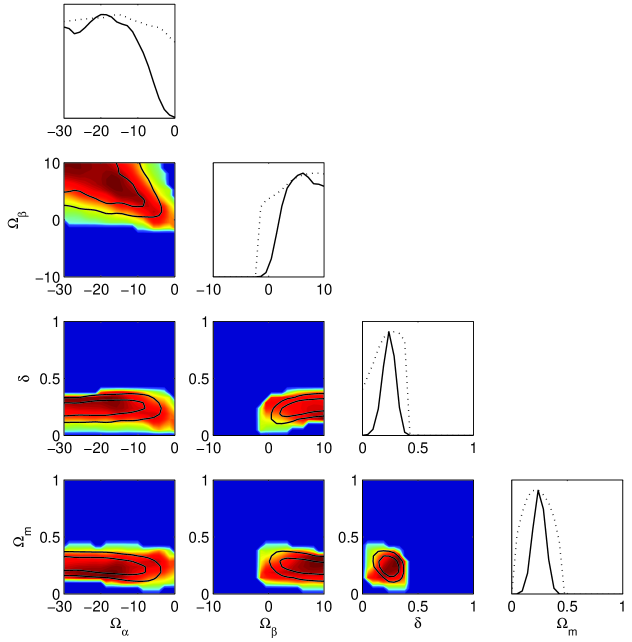
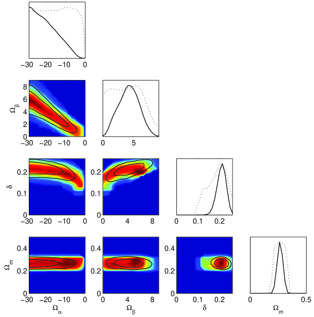
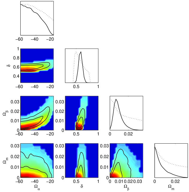
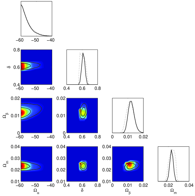
At the fig. 1, 3, 2, 4 we show constraints of the parameters of our models. In the 2D plots solid lines are the 68% and 95% confidence intervals from the marginalized probabilities. The colors reflect the mean likelihood of the sample. In the 1D plots solid lines show marginalized probabilities of the sample, dotted lines are mean likelihood. It is seen that it’s not possible to constrain properly parameter using available data (cf. table 1).
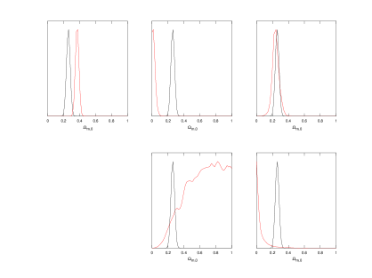
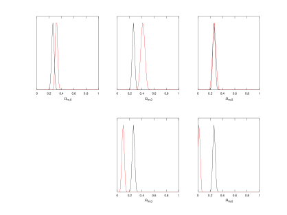
It is interesting to compare (Fig 5) a posterior probability density functions of for new models with the one for CDM model (see table 3 for the corresponding best fit values and credible intervals). As one can conclude only for model (all three parameters fitted with and without CMB data) it remains at the same level when compared with CDM model. It should be remarked that in some cases, best fit value for is small and close to the well-known amount of barionic matter (cf. table 3 row no 1, 5, 10, 11).
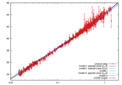
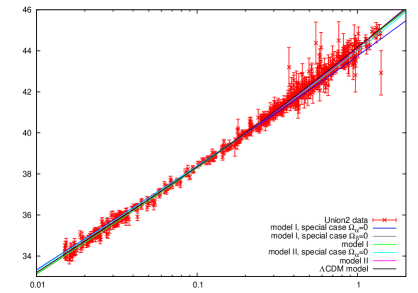
Finally, at the fig 6 Hubble’s diagrams for all our models are shown and compared with CDM. Most of them are practically indistinguishable from the concordance model on the level of Hubble diagrams. Moreover, the test gives mostly comparable results and in few cases priority belongs to new models provided that CMB data are neglected. It is clearly seen that only for the special case (fitting made with and without CMB data), the corresponding plots considerable differ from all remaining ones. These motivates us for further analysis and employing Bayesian model selection methods.
7 Models comparison and selection
Bayesian theory enables to compare investigated models, i.e. enables to show which one is the best (most probable) in the light of analysed data. Let us consider the posterior probability for model indexed by ():
| (7.1) |
is the prior probability for the model under investigation, is normalization constant, is the marginalized likelihood (also called evidence) and is given by:
| (7.2) |
It is convenient to choose the base model and compare all models from investigated set with respect to this base model by considering the ratio of posterior probabilities (posterior odds):
When all considered models are equally prior probable the posterior odds is reduced to the evidence ratio, so called Bayes Factor (). Its value can be simply interpreted as the strength of evidence in favour of base model : as inconclusive, as weak, as moderate and as strong evidence. Since the negative values of should be interpreted in favour of model under investigation.
In Table 2 one can find values of logarithm of Bayesian Factor for new models, which were calculated with respect to the base CDM model using CosmoNest code. The values were averaged from five runs.
As one can generally conclude models based on solution II are not supported by data used in analysis: we found weak and strong evidence in favor of CDM model (for both with and without CMB data cases). When considering Model one can find out that there is weak evidence in favor of it with respect to CDM model in the light of observations from late Universe. When information from early Universe is included, i.e. CMB data point is taken into account, the conclusion change: moderate evidence is found in favor of CDM model. Amazingly, the special case of quadratic gravity () is not supported by the data, in both cases the evidence in favor of the base model is strong. The result for model is inconclusive when the data from late Universe are considered. Admitting information from CMB gives us strong evidence in favor of CDM model.
| Model | Estimation without CMB data | Estimation with CMB data | ||
|---|---|---|---|---|
| CDM | 0 | 0 | ||
8 Phase space descriptions of model dynamics
Having fixed free parameters of our models on can think about their dynamical properties encoded in a time evolution of the scale factor. In fact, the dynamics of our models is determined by very complicated Friedmann type equations which constitute first order ordinary (non-linear) autonomous differential equations on the scale factor. Moreover r.h.s. of the generalized Friedmann equation (4.5,5.5) is rather rational than polynomial function (cf. (3.3)) of . While obtaining exact solutions of these equations is very difficult (if possible at all) it is enough to apply qualitative and numerical methods of analysis of differential equations. The main goal of this method is instead of studying individual trajectories of the system under consideration to describe a geometrical structure of a phase space. The main advantage is the possibility of investigating entire evolution, represented by trajectories in the phase space, for all admissible initial conditions. The phase space (the phase plane in our case) is organized through critical points and trajectories. As a result we obtain a global phase portrait of the system illustrating the stability of special solutions as well as its generic properties among all evolutional paths in the phase space.
It would be useful to represent the dynamics of the cosmological models in terms of dynamical system theory. For this aim let us re-parametrize the original time variable in (4.5,5.5) to the new re-scaled variable, say such that and define an effective potential function . Then we obtain that dynamics is reduced to the dynamics of a fictitious particle of unit mass moving on a half line in the effective potential with energy level , where is the spatial curvature index (for generality one considers models which are not flat):
| (8.1) |
The system is defined in the part of the configuration space in which is non-negative. Therefore the dynamics of cosmological model is governed by dynamical system
| (8.2) | ||||
| (8.3) |
of Newtonian type. Critical points of this system correspond to extremes on a diagram of the effective potential. Because the stability of the critical point depends on the eigenvalues of a linearization matrix (solutions of the characteristic equation) calculated at this point one obtains two possibilities (a trace of the linearization matrix is always vanishing). If one has a maximum then the critical point is a saddle. In contrast a minimum on the diagram of the potential function means that we have a center type of critical point. Critical points provide stationary solutions: stable for minimum and unstable otherwise.
In fact dynamics of the system can be read off from the graph of potential function itself (in cosmological setting the effective potential is non-positive: ). Since conservation of (total) energy holds, each trajectory is labeled by some energy level (might be negative). The difference is equal to kinetic energy and provides information about the velocity of cosmic expansion: increasing values of the potential are slowing down the evolution. Because of this the region below potential plot is forbidden for the motion. Particularly, points on the graph are turning points. For example, models with a classical bounce contract to some minimal value of the scale factor and then after approaching this value expand (to infinity). Oscillating models are, therefore, result of a potential cavity. As a result one can simply obtain different types of evolutions admissible by different values of energy levels. For example, as it was mentioned above, different choice of spatial curvature index will determine different cosmic evolution. Such visualization is complementary to the one which offers phase portrait.
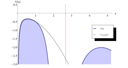
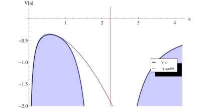
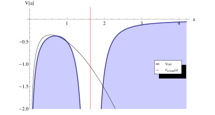
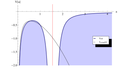
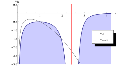
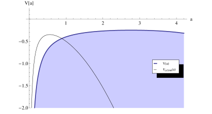
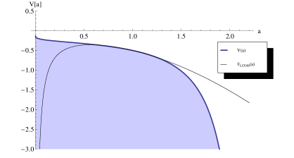
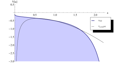
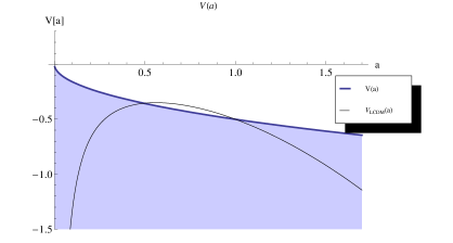
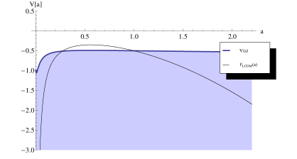
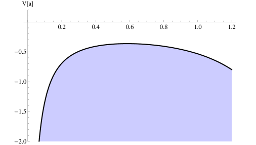
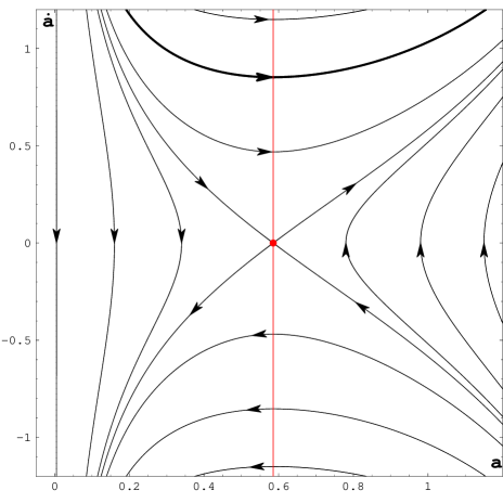
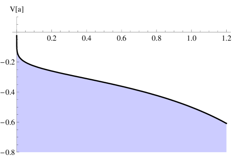
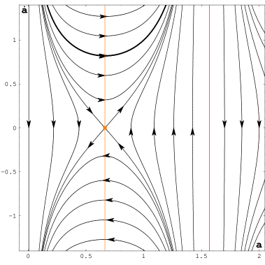
On the diagrams we have illustrated the effective potential functions (Fig. 7, 9, 8, 10, 11) as well as generic samples of phase portraits for our models (Fig. 12, 13). We found that although analytical formulae for effective potential functions for various model are very different their numerical values and therefore a shape of the corresponding graph might be almost the same. As it was explained above similar shapes give rise to similar dynamical behavior. This is what happens in our case.
.

.
Let us discuss the plots of the effective potentials for new models in more details. The model has reached very good numerical agreement with CDM for a wide range of the scale factor : from the very beginning till the present time (fig. 7). After Big Bang the universe expansion slows down (deceleration epoch) till some critical value (equal to static solution) and since then speeds up. This cosmic acceleration lasts forever for the case of CDM. In contrast, the model predicts finite size future singularity since the effective potential function (as well as velocity plot) has a pole at . It can be shown that this pole has to be reached at finite time. Therefore it is known as a sudden future singularity [38]. In the case of quadratic gravity (), the shape of the potential function is the same as for model with poorer numerical coincidence with CDM (fig. 8): . The initial deceleration era characteristic for CDM model is absent only for the case of model which offers a model of permanently accelerating universe of bouncing type. After a short period of strong acceleration (possible inflation) there is an era of low acceleration followed by CDM epoch. A characteristic for models and CDM saddle point is not present for the case of model . Finite size future singularity of the potential function appears at . However on the Hubble diagrams differences between CDM and models , and , are negligible. Similarity to CDM is lost for both models with (see fig. 9, 11) which makes this case difficult to accept. Models of modified gravity enlarge zoo of possible cosmic evolutions because of the presence of finite time final size singularity of the potential function at some finite value of the scale factor.
9 Other analysis and diagnostics
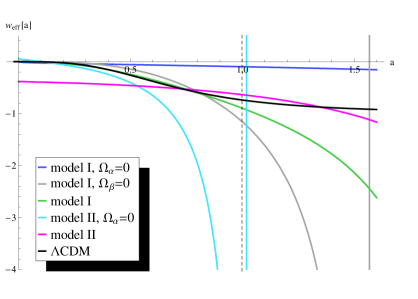
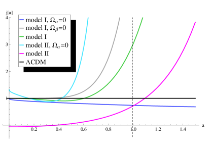
In this paper we have studied and confronted against astrophysical data as well as against the standard CDM model five cosmological models obtained from two solutions presented in Sections 4, 5. For a deeper examination and comparison of properties of our models we have used various cosmological parameters as: deceleration parameter , effective equation of state , JERK , SNAP (see e.g. [39, 40]). For a later convenience we shall express them in terms of the effective potential
| (9.1) |
| (9.2) |
| (9.3) |
| (9.4) |
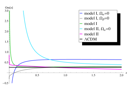
where . Therefore, explicit analytic form of the potential function is also helpful for determination of these diagnostics. Below we shall summarize the results of our analysis, for details see fig. 14, 15, 16.
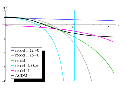
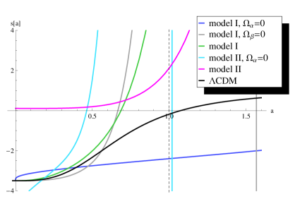
Deceleration parameter for CDM, in contrast to other models, goes asymptotically to . However, the present day values of for new models are not much different, particulary . Only for two models with the present day values o are visibly greater (see fig. 14 and table 3). One notices that the values of are almost the same at the point for all of the models except the ones with . At the beginning for all models except for which one has instead. It means a matter dominated epoch at the beginning of cosmic evolution (cf. below for plots of ).
Very similar situation is for effective equation of state parameter since it is algebraically related to (cf. (9.2)). For CDM model and (see bottom fig. 14). At there is . This explicitly indicates early matter dominated epoch noticed already before for these models.
As it can be seen on the fig. 15, that JERK parameter for CDM model is constant and for models , and approximate this value. Similarly, is also constant. From the figure one can see that different models predict different present-day values of JERK and SNAP. Unfortunately estimations of these parameters are beyond our present observational possibilities. However some recent analysis support the current values of jerk bigger than 2 [40].
In order to better understand properties of our models we shall use diagnostic from [41]:
| (9.5) |
which is designed to answer the question of nature of dark energy. For CDM model we have (see black line on fig. 16) which means that cosmological constant is the best description of dark energy. For the model the function is increasing what means that the best model for dark energy is provided by a phantom. Remaining models have decreasing function and therefore they are of quintessence type. However, one can notice that two models and have a long period of being of cosmological constant type.
10 Summary and conclusions
In this paper we have found, and then analyzed by fitting to experimental data, two families of cosmological models based on two different solutions of Palatini modified gravity equipped with non-minimal curvature coupling to (free) scalar dilaton-like field. We assume Cosmological Principle to hold and standard spatially flat FRW metric with dust matter as a source. Our analysis reveals how rich is class of cosmological models offered by modified gravity. Beside of two main models denoted respectively as and we have investigated three special cases , and corresponding to reduced lagrangian functions. Particularly, as a by-product, we have employed quadratic a la’ Starobinsky gravity, , for description of the cosmic acceleration. All models labeled by correspond to the solution (4.1) which is the same solution as in Einstein gravity provided with FRW metric and dust matter. In the case of standard gravity this solution leads, after solving Friedmann equation, to decelerating expansion. Modification of gravitational Lagrangian (e.g. by adding cosmological constant) modifies Friedmann equation and thence give rise to accelerating expansion. In contrast, models labeled by are based on the solution (5.1) which has no correspondence to standard gravity. Therefore the limit cannot be performed. Having estimated models parameters by using recent astrophysical data one has demonstrated that different models become in a good agreement with the data. We have also performed various comparative analysis against CDM concordance model which is commonly accepted as a best fitted model.
The first model , in spite of much more complicated Friedmann equation, qualitatively and quantitatively mimics the CDM one () from the very beginning of cosmic evolution (Big Bang) until the recent time. As it can be seen, on various plots, effective potential, deceleration and effective equation of state parameters (fig. 7, 14) are almost the same until the present time (). Differences appear for diagnostics employing third and forth order derivatives of the scale factor (fig 15). These properties would be helpful for future discrimination between models. Both models exhibit existence of the initial singularity, but in contrast to CDM, our model predicts the (final) finite-size sudden (finite-time) singularity at the point . The effective potential for our model has one maximum at the point which corresponds to saddle critical point at the phase portrait (see fig 12) and representing Einstein’s static solution in full analogy with CDM. For the present time the deceleration parameter and are within the expected estimations. The Hubble diagram for this case is practically indistinguishable from CDM diagram, cf. Fig. 6. Moreover, the estimation with CMB data added does not provide any essential (qualitative nor quantitative) changes to this model.
At the fig. 5 are shown posterior probability density functions for parameter for all of our models. It’s clearly seen that density function for model I almost entirely overlaps such function for CDM model (see also table 3 for the corresponding best fit values of ). One can also see that inclusion to our estimations CMB data makes possible proper estimation of for the following cases: , and II. In particular, for models II amount of is one order less than for CDM and it has the order of barionic matter.
The second our model gives rise to permanently accelerating Universe without initial singularities: Big Bang scenario is replaced by Big Bounce. The potential plot has no maximum and there is no saddle point at the phase portrait (fig 12). The lack of the initial singularity is the main advantage of this model in comparison with CDM model. The coincidence with CDM effective potential holds for . The acceleration parameter is almost linear for the scale factor near zero. The potential function indicates big slope for the scale factor near zero what can be interpreted as inflationary era. Effective equation of state at the beginning is close to (fig 14), which corresponds to domination of the spatial curvature at the initial phase of Universe’s evolution. For the present time the deceleration parameter and effective equation of state . Generic finite time finite size singularity has appear at . Again, on the level of Hubble diagram, one cannot distinguish it from CDM model.
.
In this work we have also examined the significance of the Starobinsky’s term. It appears, and can be seen on the plots of the potentials (fig 9, 11) and on the Hubble’s diagram (fig 6), that without this term the remaining parameters of the model cannot be properly fitted. Quadratic gravity along well qualitatively mimics CDM model till the present time (see fig. (8, 17)). However combining it with the non-minimally coupled scalar field provides fine tuning and much better adjustment to the concordance model. It is also to be observed that the parameter is negative provided that . In contrast for one has which provides the so-called Chameleon effect [42]. We have no at the moment good explanation for this and the problem will be studded in our future work.
The Bayesian framework of model selection has been used for comparison theoretical models with the concordance CDM one. We investigated Bayes Factor to show which model is the best (most probable) in the light of the astronomical data. We have found that while some special cases of theoretical models becomes a weak evidence in favor of it over CDM if observations from current epoch are used (SN, H(z), BAO data). Inclusion of the information coming from early epochs (CMB data ) changes this situation because we obtain strong evidence in favor of Standard Cosmological Model.
Our investigations here have aimed to distinguish the favorable model by cosmography of the FLRW background metric in the sample of theoretical models. Because of plenitude of dynamical scenarios, an introductory selection of sample of theoretical models was necessary and it accounts in final Bayesian inference. In the Bayesian framework adding of new observations is natural for improving models parameters. It means that the effects of cosmological perturbations in this class of models have not been considered here and this important task is postponed for future investigations. This will allow to enlarge the discriminatory tools for further analysis. For example, a sound speed of the fluctuations for the quadratic gravity model as calculated in [24] is
| (10.1) |
which in our case yields a superluminal value . Thus such a model should be, in principle, rejected. The dynamics of cosmological perturbations in extended gravity models, including Palatini formulation, have been studied in number of papers (see e.g. [43] and references therein) both for a matter density as well as for the background metric. However the contributions coming from non-minimal dilaton-curvature couplings one deals here have not been developed yet (cf. [44] in the context of other scalar-tensor theories) and will be a subject of our future investigations.
Acknowledgments
A.B. gratefully acknowledges interesting discussions with G. Allemandi, S. Capozziello, M. Francaviglia and S. Odintsov during a preliminary stage of this project. A.B. is supported by the Polish NCN grant 2011/B/S12/03354.
References
-
[1]
S. Perlmutter et al. [ Supernova Cosmology Project Collaboration ],
“Measurements of Omega and Lambda from 42 high redshift supernovae,”
Astrophys. J. 517, 565-586 (1999).
[astro-ph/9812133];
A. G. Riess et al. [ Supernova Search Team Collaboration ], “Observational evidence from supernovae for an accelerating universe and a cosmological constant,” Astron. J. 116, 1009-1038 (1998). [astro-ph/9805201]. -
[2]
S. M. Carroll,
“The Cosmological constant,”
Living Rev. Rel. 4, 1 (2001).
[astro-ph/0004075];
N. Straumann, “On the cosmological constant problems and the astronomical evidence for a homogeneous energy density with negative pressure,” In *Duplantier, B. (ed.) et al.: Vacuum energy, renormalization* 7-51. [astro-ph/0203330];
T. Padmanabhan, “Cosmological constant: The Weight of the vacuum,” Phys. Rept. 380, 235-320 (2003). [hep-th/0212290];
V. Sahni, “Dark matter and dark energy,” Lect. Notes Phys. 653, 141-180 (2004). [astro-ph/0403324];
E. J. Copeland, M. Sami, S. Tsujikawa, “Dynamics of dark energy,” Int. J. Mod. Phys. D15, 1753-1936 (2006). [hep-th/0603057];
M. Li, X. -D. Li, S. Wang, Y. Wang, “Dark Energy,” Commun. Theor. Phys. 56, 525-604 (2011). [arXiv:1103.5870 [astro-ph.CO]]. T. Clifton, P. G. Ferreira, A. Padilla, C. Skordis, “Modified Gravity and Cosmology,” [arXiv:1106.2476 [astro-ph.CO]];
-
[3]
S. Nojiri, S. D. Odintsov,
“Modified gravity with negative and positive powers of the curvature: Unification of the inflation and of the cosmic acceleration,”
Phys. Rev. D68, 123512 (2003).
[hep-th/0307288];
S. Nojiri, S. D. Odintsov, “Modified gravity with ln R terms and cosmic acceleration,” Gen. Rel. Grav. 36, 1765-1780 (2004). [hep-th/0308176];
S. Nojiri, S. D. Odintsov, “The Minimal curvature of the universe in modified gravity and conformal anomaly resolution of the instabilities,” Mod. Phys. Lett. A19, 627-638 (2004). [hep-th/0310045]. -
[4]
S. Nojiri, S. D. Odintsov,
“Introduction to modified gravity and gravitational alternative for dark energy,”
[hep-th/0601213];
S. Capozziello, M. Francaviglia, “Extended Theories of Gravity and their Cosmological and Astrophysical Applications,” Gen. Rel. Grav. 40, 357-420 (2008). [arXiv:0706.1146 [astro-ph]];
A. De Felice, S. Tsujikawa, “f(R) theories,” Living Rev. Rel. 13, 3 (2010). [arXiv:1002.4928 [gr-qc]];
T. P. Sotiriou, V. Faraoni, “f(R) Theories Of Gravity,” Rev. Mod. Phys. 82, 451-497 (2010). [arXiv:0805.1726 [gr-qc]];
S. Nojiri, S. D. Odintsov, “Unified cosmic history in modified gravity: from F(R) theory to Lorentz non-invariant models,” Phys. Rept. 505, 59-144 (2011). [arXiv:1011.0544 [gr-qc]];
S. Tsujikawa, “Modified gravity models of dark energy,” Lect. Notes Phys. 800, 99-145 (2010). [arXiv:1101.0191 [gr-qc]];
S. Capozziello, M. De Laurentis, “Extended Theories of Gravity,” [arXiv:1108.6266 [gr-qc]]. - [5] G. J. Olmo, “Palatini Approach to Modified Gravity: f(R) Theories and Beyond,” Int. J. Mod. Phys. D 20, 413 (2011). [arXiv:1101.3864 [gr-qc]].
-
[6]
G. J. Olmo and H. Sanchis-Alepuz,
“Hamiltonian Formulation of Palatini f(R) theories a la Brans-Dicke,”
Phys. Rev. D 83, 104036 (2011).
[arXiv:1101.3403 [gr-qc]];
G. J. Olmo, H. Sanchis-Alepuz, S. Tripathi, “Enriched Phenomenology in Extended Palatini Theories,” [arXiv:1002.3920 [gr-qc]];
C. Barragan, G. J. Olmo and H. Sanchis-Alepuz, “Avoiding the Big Bang Singularity with Palatini f(R) Theories,” [arXiv:1002.3919 [gr-qc]];
M. Campista, B. Santos, J. Santos and J. S. Alcaniz, “Cosmological Consequences of Exponential Gravity in Palatini Formalism,” Phys. Lett. B 699, 320 (2011). [arXiv:1012.3943 [astro-ph.CO]];
F. Bauer, “Filtering out the cosmological constant in the Palatini formalism of modified gravity,” Gen. Rel. Grav. 43, 1733-1757 (2011). [arXiv:1007.2546 [gr-qc]];
G. J. Olmo, H. Sanchis-Alepuz and S. Tripathi, “Enriched Phenomenology in Extended Palatini Theories,” [arXiv:1002.3920 [gr-qc]];
S. Li, H. R. Yu and T. J. Zhang, “Statefinder diagnosis for the Palatini gravity theories,” [arXiv:1002.3867 [astro-ph.CO]];
T. Harko, T. S. Koivisto and F. S. N. Lobo, “Palatini formulation of modified gravity with a nonminimal curvature-matter coupling,” Mod. Phys. Lett. A 26, 1467 (2011). [arXiv:1007.4415 [gr-qc]];
S. Capozziello, F. Darabi and D. Vernieri, “Equivalence between Palatini and metric formalisms of f(R)-gravity by divergence free current,” Mod. Phys. Lett. A 26, 65 (2011). [arXiv:1006.0454 [gr-qc]];
T. Koivisto, “Viable Palatini-f(R) cosmologies with generalized dark matter,” Phys. Rev. D 76, 043527 (2007). [arXiv:0706.0974 [astro-ph]];
-
[7]
M. Ferraris, M. Francaviglia, I. Volovich,
“Universal gravitational equations,”
Nuovo Cim. B108, 1313-1317 (1993);
M. Ferraris, M. Francaviglia, I. Volovich, “The Universality of vacuum Einstein equations with cosmological constant,” Class. Quant. Grav. 11, 1505-1517 (1994). [gr-qc/9303007];
A. Borowiec, M. Ferraris, M. Francaviglia, I. Volovich, “Universality of Einstein equations for the Ricci squared Lagrangians,” Class. Quant. Grav. 15, 43-55 (1998). [arXiv:gr-qc/9611067 [gr-qc]];
A. Borowiec, M. Francaviglia, I. Volovich, “Topology change and signature change in non-linear first-order gravity,” Int. J. Geom. Meth. Mod. Phys. 4, 647-667 (2007). -
[8]
G. Allemandi, A. Borowiec, M. Francaviglia,
“Accelerated cosmological models in first order nonlinear gravity,”
Phys. Rev. D70, 043524 (2004).
[arXiv:hep-th/0403264 [hep-th]];
G. Allemandi, A. Borowiec, M. Francaviglia, “Accelerated cosmological models in Ricci squared gravity,” Phys. Rev. D70, 103503 (2004). [arXiv:hep-th/0407090 [hep-th]]. -
[9]
S. Nojiri, S. D. Odintsov,
“Gravity assisted dark energy dominance and cosmic acceleration,”
Phys. Lett. B599, 137-142 (2004).
[astro-ph/0403622];
G. Allemandi, M. Francaviglia, M. L. Ruggiero, A. Tartaglia, “Post-Newtonian parameters from alternative theories of gravity,” Gen. Rel. Grav. 37, 1891-1904 (2005). [gr-qc/0506123]. - [10] A. Borowiec, “From Dark Energy to Dark Matter via Non-Minimal Coupling,” [arXiv:0812.4383 [gr-qc]].
-
[11]
O. Bertolami, J. Paramos,
“On the non-trivial gravitational coupling to matter,”
Class. Quant. Grav. 25, 245017 (2008).
[arXiv:0805.1241 [gr-qc]];
O. Bertolami, J. Paramos, T. Harko, F. S. N. Lobo, “Non-minimal curvature-matter couplings in modified gravity,” [arXiv:0811.2876 [gr-qc]];
O. Bertolami, P. Frazao, J. Paramos, “Reheating via a generalized non-minimal coupling of curvature to matter,” Phys. Rev. D83, 044010 (2011). [arXiv:1010.2698 [gr-qc]];
J. Paramos, O. Bertolami, “Mimicking the cosmological constant: constant curvature spherical solutions in a non-minimally coupled model,” [arXiv:1107.0225 [gr-qc]]. - [12] S. Nojiri, S. D. Odintsov, P. V. Tretyakov, “From inflation to dark energy in the non-minimal modified gravity,” Prog. Theor. Phys. Suppl. 172, 81-89 (2008). [arXiv:0710.5232 [hep-th]].
- [13] D. Puetzfeld and Y. N. Obukhov, “On the motion of test bodies in theories with non-minimal coupling,” Phys. Rev. D 78, 121501 (2008). [arXiv:0811.0913 [astro-ph]].
- [14] R. Amanullah et al., “Spectra and Light Curves of Six Type Ia Supernovae at 0.511 ¡ z ¡ 1.12 and the Union2 Compilation,” Astrophys. J. 716, 712 (2010). [arXiv:1004.1711 [astro-ph.CO]].
- [15] J. Simon, L. Verde, R. Jimenez, “Constraints on the redshift dependence of the dark energy potential,” Phys. Rev. D71, 123001 (2005). [astro-ph/0412269].
-
[16]
D. J. Eisenstein et al. [ SDSS Collaboration ],
“Detection of the baryon acoustic peak in the large-scale correlation function of SDSS luminous red galaxies,”
Astrophys. J. 633, 560-574 (2005).
[astro-ph/0501171];
W. J. Percival, S. Cole, D. J. Eisenstein, R. C. Nichol, J. A. Peacock, A. C. Pope, A. S. Szalay, “Measuring the Baryon Acoustic Oscillation scale using the SDSS and 2dFGRS,” Mon. Not. Roy. Astron. Soc. 381, 1053-1066 (2007). [arXiv:0705.3323 [astro-ph]];
B. A. Reid et al. [ SDSS Collaboration ], “Baryon Acoustic Oscillations in the Sloan Digital Sky Survey Data Release 7 Galaxy Sample,” Mon. Not. Roy. Astron. Soc. 401, 2148-2168 (2010). [arXiv:0907.1660 [astro-ph.CO]]. - [17] E. Komatsu et al. [ WMAP Collaboration ], “Seven-Year Wilkinson Microwave Anisotropy Probe (WMAP) Observations: Cosmological Interpretation,” Astrophys. J. Suppl. 192, 18 (2011). [arXiv:1001.4538 [astro-ph.CO]].
- [18] http://cosmonest.org/
-
[19]
S. Capozziello, V. F. Cardone, M. Francaviglia,
“f(R) Theories of gravity in Palatini approach matched with observations,”
Gen. Rel. Grav. 38, 711-734 (2006).
[astro-ph/0410135];
T. P. Sotiriou, “Constraining f(R) gravity in the Palatini formalism,” Class. Quant. Grav. 23, 1253-1267 (2006). [gr-qc/0512017];
M. Amarzguioui, O. Elgaroy, D. F. Mota, T. Multamaki, “Cosmological constraints on f(r) gravity theories within the palatini approach,” Astron. Astrophys. 454, 707-714 (2006). [astro-ph/0510519];
A. Borowiec, W. Godlowski, M. Szydlowski, “Accelerated cosmological models in modified gravity tested by distant supernovae snia data,” Phys. Rev. D74, 043502 (2006). [astro-ph/0602526];
A. Borowiec, W. Godlowski, M. Szydlowski, “Dark matter and dark energy as a effects of Modified Gravity,” [astro-ph/0607639];
S. Fay, R. Tavakol and S. Tsujikawa, “f(R) gravity theories in Palatini formalism: Cosmological dynamics and observational constraints,” Phys. Rev. D 75, 063509 (2007). [arXiv:astro-ph/0701479]. - [20] R. Wojtak, S.H. Hansen, J. Hjorth, “Gravitational redshift of galaxies in clusters as predicted by general relativity,“ Nature 477:567-569 (2011) [arXiv:1109.6571 [astro-ph.CO]].
- [21] R. Trotta, “Bayes in the sky: Bayesian inference and model selection in cosmology,” Contemp. Phys. 49, 71 (2008) [arXiv:0803.4089 [astro-ph]].
- [22] T. Koivisto, “Covariant conservation of energy momentum in modified gravities,” Class. Quant. Grav. 23, 4289-4296 (2006). [gr-qc/0505128].
-
[23]
A. A. Starobinsky,
“Isotropization of arbitrary cosmological expansion given an effective cosmological constant,”
JETP Lett. 37, 66-69 (1983);
A. A. Starobinsky, “A New Type of Isotropic Cosmological Models Without Singularity,” Phys. Lett. B91, 99-102 (1980). - [24] T. S. Koivisto, “Bouncing Palatini cosmologies and their perturbations,” Phys. Rev. D 82, 044022 (2010). [arXiv:1004.4298 [gr-qc]].
-
[25]
G. F. R. Ellis, J. Murugan, C. G. Tsagas,
“The Emergent universe: An Explicit construction,”
Class. Quant. Grav. 21, 233-250 (2004).
[gr-qc/0307112];
D. Muller and S. D. P. Vitenti, “About Starobinsky inflation,” Phys. Rev. D 74, 083516 (2006). [arXiv:gr-qc/0606018];
C. Corda, “An oscillating Universe from the linearized theory of gravity,” Gen. Rel. Grav. 40, 2201-2212 (2008). [arXiv:0802.2523 [astro-ph]];
G. J. Olmo, “Palatini Actions and Quantum Gravity Phenomenology,” [arXiv:1101.2841 [gr-qc]];
C. Corda, H. J. Mosquera Cuesta, R. L. Gomez, “High-energy scalarons in gravity as a model for Dark Matter in galaxies,” [arXiv:1105.0147 [gr-qc]];
F. Bauer, “The cosmological constant filter without big bang singularity,” [arXiv:1108.0875 [gr-qc]]. - [26] M. Kowalski et al. [ Supernova Cosmology Project Collaboration ], “Improved Cosmological Constraints from New, Old and Combined Supernova Datasets,” Astrophys. J. 686, 749-778 (2008). [arXiv:0804.4142 [astro-ph]].
- [27] J. A. Holtzman, J. Marriner, R. Kessler, M. Sako, B. Dilday, J. A. Frieman, D. P. Schneider, B. Bassett et al., “The Sloan Digital Sky Survey-II Photometry and Supernova IA Light Curves from the 2005 Data,” Astron. J. 136, 2306-2320 (2008). [arXiv:0908.4277 [astro-ph.CO]].
- [28] M. Hicken, W. M. Wood-Vasey, S. Blondin, P. Challis, S. Jha, P. L. Kelly, A. Rest, R. P. Kirshner, “Improved Dark Energy Constraints from 100 New CfA Supernova Type Ia Light Curves,” Astrophys. J. 700, 1097-1140 (2009). [arXiv:0901.4804 [astro-ph.CO]].
- [29] D. Stern, R. Jimenez, L. Verde, M. Kamionkowski, S. A. Stanford, “Cosmic Chronometers: Constraining the Equation of State of Dark Energy. I: H(z) Measurements,” JCAP 1002, 008 (2010). [arXiv:0907.3149 [astro-ph.CO]].
- [30] E. Gaztanaga, A. Cabre, L. Hui, “Clustering of Luminous Red Galaxies IV: Baryon Acoustic Peak in the Line-of-Sight Direction and a Direct Measurement of H(z),” Mon. Not. Roy. Astron. Soc. 399, 1663-1680 (2009). [arXiv:0807.3551 [astro-ph]].
- [31] J. R. Bond, G. Efstathiou, M. Tegmark, “Forecasting cosmic parameter errors from microwave background anisotropy experiments,” Mon. Not. Roy. Astron. Soc. 291, L33-L41 (1997). [astro-ph/9702100].
- [32] T. M. Davis, E. Mortsell, J. Sollerman, A. C. Becker, S. Blondin, P. Challis, A. Clocchiatti, A. V. Filippenko et al., “Scrutinizing Exotic Cosmological Models Using ESSENCE Supernova Data Combined with Other Cosmological Probes,” Astrophys. J. 666, 716-725 (2007). [astro-ph/0701510].
- [33] A. G. Riess et al., “A Redetermination of the Hubble Constant with the Hubble Space Telescope from a Differential Distance Ladder.” Astrophys. J. 699, 539 (2009). [arXiv:0905.0695 [astro-ph.CO]].
- [34] P. Mukherjee, D. Parkinson, A. R. Liddle, “A nested sampling algorithm for cosmological model selection,” Astrophys. J. 638, L51-L54 (2006). [astro-ph/0508461].
- [35] P. Mukherjee, D. Parkinson, P. S. Corasaniti, A. R. Liddle, M. Kunz, “Model selection as a science driver for dark energy surveys,” Mon. Not. Roy. Astron. Soc. 369, 1725-1734 (2006). [astro-ph/0512484].
- [36] D. Parkinson, P. Mukherjee, A.R. Liddle, “A Bayesian model selection analysis of WMAP3,” Phys. Rev. D73, 123523 (2006). [astro-ph/0605003].
- [37] D. L. Wiltshire, “Gravitational energy as dark energy: Cosmic structure and apparent acceleration,” [arXiv:1102.2045 [astro-ph.CO]].
-
[38]
Y. Shtanov and V. Sahni,
“Unusual cosmological singularities in brane world models,”
Class. Quant. Grav. 19, L101 (2002)
[arXiv:gr-qc/0204040];
J. D. Barrow, “Sudden future singularities,” Class. Quant. Grav. 21, L79-L82 (2004). [gr-qc/0403084];
S. Nojiri, S. D. Odintsov, S. Tsujikawa, “Properties of singularities in (phantom) dark energy universe,” Phys. Rev. D71, 063004 (2005). [hep-th/0501025];
P. Tretyakov, A. Toporensky, Y. Shtanov, V. Sahni, “Quantum effects, soft singularities and the fate of the universe in a braneworld cosmology,” Class. Quant. Grav. 23, 3259-3274 (2006). [gr-qc/0510104]. -
[39]
V. Sahni, T. D. Saini, A. A. Starobinsky and U. Alam,
“Statefinder: A New geometrical diagnostic of dark energy,”
JETP Lett. 77, 201 (2003)
[Pisma Zh. Eksp. Teor. Fiz. 77, 249 (2003)]
[arXiv:astro-ph/0201498];
U. Alam, V. Sahni, T. D. Saini, A. A. Starobinsky, “Exploring the expanding universe and dark energy using the Statefinder diagnostic,” Mon. Not. Roy. Astron. Soc. 344, 1057 (2003). [astro-ph/0303009];
M. Visser, “Jerk and the cosmological equation of state,” Class. Quant. Grav. 21, 2603-2616 (2004). [gr-qc/0309109];
Y. .L. Bolotin, O. A. Lemets, D. A. Yerokhin, “Expanding Universe: slowdown or speedup?,” [arXiv:1108.0203 [astro-ph.CO]]. - [40] D. Rapetti, S. W. Allen, M. A. Amin, R. D. Blandford, “A kinematical approach to dark energy studies,” Mon. Not. Roy. Astron. Soc. 375, 1510-1520 (2007). [astro-ph/0605683].
- [41] V. Sahni, A. Shafieloo, A. A. Starobinsky, “Two new diagnostics of dark energy,” Phys. Rev. D78, 103502 (2008). [arXiv:0807.3548 [astro-ph]].
-
[42]
J. Khoury and A. Weltman,
“Chameleon Fields: Awaiting Surprises for Tests of Gravity in Space,”
Phys. Rev. Lett. 93, 171104 (2004).
[arXiv:astro-ph/0309300];
J. Khoury and A. Weltman, “Chameleon Cosmology,” Phys. Rev. D 69, 044026 (2004). [arXiv:astro-ph/0309411];
T. Faulkner, M. Tegmark, E. F. Bunn and Y. Mao, “Constraining f(R) gravity as a scalar tensor theory,” Phys. Rev. D 76, 063505 (2007). [arXiv:astro-ph/0612569]. -
[43]
K. Uddin, J. ELidsey and R. Tavakol,
“Cosmological perturbations in Palatini modified gravity,”
Class. Quant. Grav. 24, 3951 (2007)
[arXiv:0705.0232 [gr-qc]];
Y. Gong, “The growth factor parameterization and modified gravity,” Phys. Rev. D 78, 123010 (2008) [arXiv:0808.1316 [astro-ph]];
H. Wei, “Growth Index of DGP Model and Current Growth Rate Data,” Phys. Lett. B 664, 1 (2008) [arXiv:0802.4122 [astro-ph]];
H. Motohashi, A. A. Starobinsky and J. ’i. Yokoyama, “Analytic solution for matter density perturbations in a class of viable cosmological f(R) models,” Int. J. Mod. Phys. D 18, 1731 (2009) [arXiv:0905.0730 [astro-ph.CO]];
S. Tsujikawa, K. Uddin and R. Tavakol, “Density perturbations in f(R) gravity theories in metric and Palatini formalisms,” Phys. Rev. D 77, 043007 (2008) [arXiv:0712.0082 [astro-ph]];
S. Tsujikawa, “Matter density perturbations and effective gravitational constant in modified gravity models of dark energy,” Phys. Rev. D 76, 023514 (2007) [arXiv:0705.1032 [astro-ph]];
S. Baghram and S. Rahvar, “Structure formation in gravity: A distinguishing probe between the dark energy and modified gravity,” JCAP 1012, 008 (2010) [arXiv:1004.3360 [astro-ph.CO]]. -
[44]
T. Koivisto and H. Kurki-Suonio,
“Cosmological perturbations in the palatini formulation of modified gravity,”
Class. Quant. Grav. 23, 2355 (2006)
[astro-ph/0509422];
N. Tamanini and C. R. Contaldi, “Inflationary Perturbations in Palatini Generalised Gravity,” Phys. Rev. D 83, 044018 (2011) [arXiv:1010.0689 [gr-qc]];
F. Bauer and D. A. Demir, “Inflation with Non-Minimal Coupling: Metric versus Palatini Formulations,” Phys. Lett. B 665, 222 (2008) [arXiv:0803.2664 [hep-ph]].
| models I: equation (4.7) - the parameters estimated without CMB data | ||||||||
| 1 | , , | - | ||||||
| 2 | , | |||||||
| 3 | , , | |||||||
| models II: equation (5.7) - the parameters estimated without CMB data | ||||||||
| 4 | , , | - | ||||||
| 5 | , , | |||||||
| model CDM: - the parameter estimated without CMB data | ||||||||
| 6 | ||||||||
| models I: equation (4.7) - the parameters estimated with CMB data added | ||||||||
| 7 | , , | |||||||
| 8 | , | |||||||
| 9 | , , | |||||||
| models II: equation (5.7) - the parameters estimated with CMB data added | ||||||||
| 10 | , , | - | ||||||
| 11 | , , | |||||||
| model CDM: - the parameter estimated with CMB data added | ||||||||
| 12 | ||||||||