\addressemail

delitsyn@mail.ru, binh-thanh.nguyen@polytechnique.edu, denis.grebenkov@polytechnique.edu

Exponential decay of Laplacian eigenfunctions in domains with branches

Andrey Delitsyn1    Binh-Thanh Nguyen2   
and Denis S. Grebenkov2-4
1 Mathematical Department of the Faculty of Physics, Moscow State University, 119991 Moscow, Russia
2 Laboratoire de Physique de la Matière Condensée (UMR 7643),
CNRS – Ecole Polytechnique, F-91128 Palaiseau, France
3 Laboratoire Poncelet, CNRS – Independent University of Moscow,
Bolshoy Vlasyevskiy Pereulok 11, 119002 Moscow, Russia
4 Chebyshev Laboratory, Saint Petersburg State University,
14th line of Vasil’evskiy Ostrov 29, Saint Petersburg, Russia
Abstract

The behavior of Laplacian eigenfunctions in domains with branches is investigated. If an eigenvalue is below a threshold which is determined by the shape of the branch, the associated eigenfunction is proved to exponentially decay inside the branch. The decay rate is twice the square root of the difference between the threshold and the eigenvalue. The derived exponential estimate is applicable for arbitrary domains in any spatial dimension. Numerical simulations illustrate and further extend the theoretical estimate.

1 Introduction

The Laplace operator eigenfunctions play a crucial role in different fields of physics: vibration modes of a thin membrane, standing waves in optical or acoustical cavity resonators, the natural spectral decomposition basis for diffusive processes, the eigenstates of a single trapped particle in quantum mechanics, etc. For the unit interval, the spectrum of the Laplace operator is particularly simple, and the eigenfunctions are just linear combinations of Fourier harmonics {eiπnx}superscript𝑒𝑖𝜋𝑛𝑥\{e^{i\pi nx}\}. The oscillating character of eigenfunctions is then often expected for domains in two and higher dimensions. The “scholar” examples of the explicit eigenbases in rectangular and circular domains strongly support this oversimplified but common view. At the same time, the geometrical structure of eigenfunctions may be extremely complicated even for simple domains (e.g., the structure of nodal lines of degenerate eigenfunctions in a square [1]). The more complex the domain is, the more sophisticated and sometimes unexpected the behavior of the associated eigenfunctions may be. For instance, numerous numerical and experimental studies of the eigenvalue problem in irregular or (pre)fractal domains revealed the existence of weakly localized eigenfunctions which have pronounced amplitudes only on small subregions of the domain [6, 5, 7, 10, 3, 4, 9, 11, 2, 8, 12, 13].

In this paper, we investigate the behavior of Laplacian eigenfunctions in domains with branches. We show that certain eigenfunctions are “expelled” from the branch, i.e., their amplitude along the branch decays exponentially fast. A similar “expulsion” effect is well known in optics and acoustics: a wave of wavelength \ell cannot freely propagate inside a rectangular channel of width b𝑏b smaller than /22\ell/2 because of the exponential attenuation exπ/bsimilar-toabsentsuperscript𝑒𝑥𝜋𝑏\sim e^{-x\pi/b} along the channel [2, 14]. We extend this classical result to arbitrary domains with branches of arbitrary shape. We derive a rigorous exponential estimate for the L2subscript𝐿2L_{2}-norm of the eigenfunction in cross-sections of the branch. We obtain the sharp decay rate which generalizes and refines the classical rate π/b𝜋𝑏\pi/b. Although this problem is remotely related to localization of waves in optical or acoustical waveguides (e.g., infinite bended tubes [14, 15, 16]), we mainly focus on bounded domains.

It is worth noting that the exponential decay of eigenfunctions of Schrödinger operators in free space (so-called strong localization) has been thoroughly investigated in physical and mathematical literature (see, e.g., [17, 18, 19, 20, 21]). The first exploration of this problem for arbitrary Schrödinger potential bounded from below was given by Schnol’ [17] who proved an exponential decay of eigenfunctions in which the decay rate was related to the distance between the corresponding eigenvalue and the essential spectrum. This result is of remarkable generality because the essential spectrum may be arbitrary, for example with gaps, and may not consist of positive axis. A sharp estimate for the decay rate was made by Maslov who reduced the problem to a differential inequality [20, 21]. Anderson discovered the exponential decay of eigenfunctions of the Schrödinger operator with random potentials [22]. This phenomenon, known as the Anderson localization, has been intensively investigated (see reviews [23, 24]). Although the Laplace operator in a bounded domain is a much simpler mathematical object, the properties of its eigenfunctions are still poorly understood.

The paper is organized as follows. In Sec. 2, we start by considering a two-dimensional domain with a rectangular branch. In this special case, the estimates are derived in a rather elementary and straightforward way that helps to illustrate many properties of eigenfunctions. Section 3 presents the analysis for domains with branches of arbitrary shape in any spatial dimension. We provide a sufficient condition on the eigenvalue, under which the related eigenfunction decays exponentially inside the branch. Sec. 4 presents numerical examples which illustrate the theoretical results and suggest new perspectives for further investigations. The paper ends by conclusions, in which the main results are summarized and their consequences are discussed.

2 Rectangular branch

Refer to caption
Figure 1: A bounded domain D𝐷D is the union of a basic domain V𝑉V of arbitrary shape and a branch Q𝑄Q. Our goal is to estimate how an eigenfunction of the Laplace operator in D𝐷D decays inside the branch. (a) rectangular branch Q={(x,y)2:0<x<a,0<y<b}𝑄conditional-set𝑥𝑦superscript2formulae-sequence0𝑥𝑎0𝑦𝑏Q=\{(x,y)\in{\mathbb{R}}^{2}~{}:~{}0<x<a,~{}0<y<b\} (the energetic norm is estimated in the subdomain Q(x0)𝑄subscript𝑥0Q(x_{0}) shown by shadowed region); (b) branch of arbitrary shape [the L2subscript𝐿2L_{2}-norm is estimated in the cross-section Ω(x)Ω𝑥\Omega(x)]; (c) three-dimensional increasing branch.

We begin with the following example. We consider the Dirichlet eigenvalue problem

Δu=λu,(x,y)D,u|D=0formulae-sequenceΔ𝑢𝜆𝑢formulae-sequence𝑥𝑦𝐷evaluated-at𝑢𝐷0-\Delta u=\lambda u,\quad(x,y)\in D,\quad\quad u|_{\partial D}=0 (1)

in a planar bounded domain D¯=V¯Q¯¯𝐷¯𝑉¯𝑄\overline{D}=\overline{V}\cup\overline{Q} which is decomposed into a basic domain V𝑉V of arbitrary shape and a rectangular branch Q𝑄Q with sides a𝑎a and b𝑏b: Q={(x,y)2:0<x<a,0<y<b}𝑄conditional-set𝑥𝑦superscript2formulae-sequence0𝑥𝑎0𝑦𝑏Q=\{(x,y)\in{\mathbb{R}}^{2}~{}:~{}0<x<a,~{}0<y<b\}, as illustrated on Fig. 1a. We assume that the eigenvalue λ𝜆\lambda is smaller than the first eigenvalue of the Laplace operator in the cross-section of the branch (i.e., the interval [0,b]0𝑏[0,b]):

λ<π2/b2.𝜆superscript𝜋2superscript𝑏2\lambda<\pi^{2}/b^{2}. (2)

Under this condition, we aim to show the exponential decay of the associated eigenfunction u𝑢u in the branch Q𝑄Q.

In this illustrative example, the derivation is based on an explicit upper bound for the norm of the eigenfunction u𝑢u. One can easily check that a general solution of Eq. (1) in the rectangular branch Q𝑄Q has a form

u(x,y)=n=1cnsinh(γn(ax))sin(πny/b),𝑢𝑥𝑦superscriptsubscript𝑛1subscript𝑐𝑛subscript𝛾𝑛𝑎𝑥𝜋𝑛𝑦𝑏u(x,y)=\sum\limits_{n=1}^{\infty}c_{n}\sinh(\gamma_{n}(a-x))\sin(\pi ny/b), (3)

where γn=(πbn)2λsubscript𝛾𝑛superscript𝜋𝑏𝑛2𝜆\gamma_{n}=\sqrt{(\frac{\pi}{b}n)^{2}-\lambda}, and cnsubscript𝑐𝑛c_{n} are constants. We consider the energetic norm of the function u𝑢u in the subdomain Q(x0)={(x,y)2:x0<x<a,0<y<b}𝑄subscript𝑥0conditional-set𝑥𝑦superscript2formulae-sequencesubscript𝑥0𝑥𝑎0𝑦𝑏Q(x_{0})=\{(x,y)\in{\mathbb{R}}^{2}~{}:~{}x_{0}<x<a,~{}0<y<b\} which is defined as

uL2(Q(x0))2Q(x0)(u,u)𝑑x𝑑y.subscriptsuperscriptnorm𝑢2subscript𝐿2𝑄subscript𝑥0subscript𝑄subscript𝑥0𝑢𝑢differential-d𝑥differential-d𝑦||\nabla u||^{2}_{L_{2}(Q(x_{0}))}\equiv\int\limits_{Q(x_{0})}(\nabla u,\nabla u)dxdy. (4)

Substituting Eq. (3) to (4) yields

uL2(Q(x0))2=n=1cn2b2x0a[(πbn)2sinh2(γn(ax))+γn2cosh2(γn(ax))]dx.subscriptsuperscriptnorm𝑢2subscript𝐿2𝑄subscript𝑥0superscriptsubscript𝑛1superscriptsubscript𝑐𝑛2𝑏2superscriptsubscriptsubscript𝑥0𝑎delimited-[]superscript𝜋𝑏𝑛2superscript2subscript𝛾𝑛𝑎𝑥subscriptsuperscript𝛾2𝑛superscript2subscript𝛾𝑛𝑎𝑥𝑑𝑥\begin{split}||\nabla u||^{2}_{L_{2}(Q(x_{0}))}&=\sum\limits_{n=1}^{\infty}c_{n}^{2}\frac{b}{2}\int\limits_{x_{0}}^{a}\biggl{[}(\frac{\pi}{b}n)^{2}\sinh^{2}(\gamma_{n}(a-x))\\ &+\gamma^{2}_{n}\cosh^{2}(\gamma_{n}(a-x))\biggr{]}dx.\\ \end{split} (5)

Using elementary inequalities for the integral (see Appendix A), one gets

uL2(Q(x0))2Ce2γ1x0n=1ncn2sinh2(γna),subscriptsuperscriptnorm𝑢2subscript𝐿2𝑄subscript𝑥0𝐶superscript𝑒2subscript𝛾1subscript𝑥0superscriptsubscript𝑛1𝑛superscriptsubscript𝑐𝑛2superscript2subscript𝛾𝑛𝑎||\nabla u||^{2}_{L_{2}(Q(x_{0}))}\leq Ce^{-2\gamma_{1}x_{0}}\sum\limits_{n=1}^{\infty}nc_{n}^{2}\sinh^{2}(\gamma_{n}a), (6)

where C𝐶C is an explicit constant. The trace theorem provides the upper bound for the above series (see Appendix A)

uL2(Q(x0))2C1e2γ1x0,subscriptsuperscriptnorm𝑢2subscript𝐿2𝑄subscript𝑥0subscript𝐶1superscript𝑒2subscript𝛾1subscript𝑥0||\nabla u||^{2}_{L_{2}(Q(x_{0}))}\leq C_{1}e^{-2\gamma_{1}x_{0}},

with another explicit constant C1subscript𝐶1C_{1}. So, we established the exponential decay of the energy u2superscriptnorm𝑢2||\nabla u||^{2} in the branch Q𝑄Q with the decay rate 2γ1=2(πb)2λ2subscript𝛾12superscript𝜋𝑏2𝜆2\gamma_{1}=2\sqrt{(\frac{\pi}{b})^{2}-\lambda}.

From this estimate it is easy to deduce a similar estimate in the L2subscript𝐿2L_{2}-norm,

uL2(Q(x0))2Q(x0)u2𝑑x𝑑yC2e2γ1x0,subscriptsuperscriptnorm𝑢2subscript𝐿2𝑄subscript𝑥0subscript𝑄subscript𝑥0superscript𝑢2differential-d𝑥differential-d𝑦subscript𝐶2superscript𝑒2subscript𝛾1subscript𝑥0||u||^{2}_{L_{2}(Q(x_{0}))}\equiv\int\limits_{Q(x_{0})}u^{2}dxdy\leq C_{2}e^{-2\gamma_{1}x_{0}}, (7)

where C2subscript𝐶2C_{2} is another constant. The derivation implies that the estimate is sharp, i.e. the decay rate cannot be improved in general.

It is worth noting that no information about the basic domain V𝑉V was used. In particular, the Dirichlet boundary condition on V𝑉\partial V can be replaced by arbitrary boundary condition under which the Laplace operator is still self-adjoint.

3 Branch of arbitrary shape

Now we show that the above estimate remains valid for eigenfunctions in a much more general case with a branch of arbitrary shape in n+1superscript𝑛1{\mathbb{R}}^{n+1} (n=1,2,3,𝑛123n=1,2,3,...). We consider the eigenvalue problem

Δu(x,𝐲)=λu(x,𝐲)(x,𝐲)D,u|D=0,formulae-sequenceΔ𝑢𝑥𝐲𝜆𝑢𝑥𝐲formulae-sequence𝑥𝐲𝐷evaluated-at𝑢𝐷0-\Delta u(x,{\bf y})=\lambda u(x,{\bf y})\quad(x,{\bf y})\in D,\quad\quad u|_{\partial D}=0, (8)

where D¯=V¯Q¯¯𝐷¯𝑉¯𝑄\overline{D}=\overline{V}\cup\overline{Q} is decomposed into a basic bounded domain Vn+1𝑉superscript𝑛1V\subset{\mathbb{R}}^{n+1} of arbitrary shape and a branch Qn+1𝑄superscript𝑛1Q\subset{\mathbb{R}}^{n+1} of a variable cross-section profile Ω(x)nΩ𝑥superscript𝑛\Omega(x)\subset{\mathbb{R}}^{n} (Fig. 1b,c):

Q={(x,𝐲)n+1:𝐲Ω(x),0<x<a}.𝑄conditional-set𝑥𝐲superscript𝑛1formulae-sequence𝐲Ω𝑥0𝑥𝑎Q=\{(x,{\bf y})\in{\mathbb{R}}^{n+1}~{}:~{}{\bf y}\in\Omega(x),~{}0<x<a\}.

Each cross-section Ω(x)Ω𝑥\Omega(x) is a bounded domain which is parameterized by x𝑥x from 00 to a𝑎a. The boundary of the branch Q𝑄Q is assumed to be piecewise smooth [25]. Although weaker conditions on the boundary could potentially be used, their justification would require a substantial technical analysis which is beyond the scope of the paper.

For a fixed x𝑥x, let μ1(x)subscript𝜇1𝑥\mu_{1}(x) be the first eigenvalue of the problem

Δϕ(𝐲)=μ1(x)ϕ(𝐲)𝐲Ω(x),ϕ|Ω=0,formulae-sequencesubscriptΔperpendicular-toitalic-ϕ𝐲subscript𝜇1𝑥italic-ϕ𝐲formulae-sequence𝐲Ω𝑥evaluated-atitalic-ϕΩ0-\Delta_{\perp}\phi({\bf y})=\mu_{1}(x)\phi({\bf y})\quad{\bf y}\in\Omega(x),\quad\quad\phi|_{\partial\Omega}=0, (9)

where ΔsubscriptΔperpendicular-to\Delta_{\perp} is the n𝑛n-dimensional Laplace operator. We denote

μ=inf0<x<aμ1(x)𝜇subscriptinfimum0𝑥𝑎subscript𝜇1𝑥\mu=\inf\limits_{0<x<a}\mu_{1}(x) (10)

the smallest first eigenvalue among all cross-sections of the branch. For example, if Ω(x)=[0,b]Ω𝑥0𝑏\Omega(x)=[0,b] (independent of x𝑥x), one has μ=π2/b2𝜇superscript𝜋2superscript𝑏2\mu=\pi^{2}/b^{2} and retrieves the example from Sec. 2.

Now, we can formulate the main result of the paper. If the basic domain V𝑉V is large enough so that

λ<μ,𝜆𝜇\lambda<\mu, (11)

we prove that the squared L2subscript𝐿2L_{2}-norm of the eigenfunction u𝑢u in the cross-section Ω(x0)Ωsubscript𝑥0\Omega(x_{0}),

I(x0)Ω(x0)u2(x0,𝐲)𝑑𝐲,𝐼subscript𝑥0subscriptΩsubscript𝑥0superscript𝑢2subscript𝑥0𝐲differential-d𝐲I(x_{0})\equiv\int\limits_{\Omega(x_{0})}u^{2}(x_{0},{\bf y})d{\bf y}, (12)

decays exponentially with x0subscript𝑥0x_{0}:

I(x0)I(0)eβx0(0x0<a),𝐼subscript𝑥0𝐼0superscript𝑒𝛽subscript𝑥00subscript𝑥0𝑎I(x_{0})\leq I(0)e^{-\beta x_{0}}\quad(0\leq x_{0}<a), (13)

with the decay rate

β=2μλ.𝛽2𝜇𝜆\beta=\sqrt{2}~{}\sqrt{\mu-\lambda}. (14)

Moreover, if the branch profile Ω(x)Ω𝑥\Omega(x) satisfies the condition

(𝐞x,𝐧(x,𝐲))0(x,𝐲)Q,formulae-sequencesubscript𝐞𝑥𝐧𝑥𝐲0for-all𝑥𝐲𝑄({\bf e}_{x},{\bf n}(x,{\bf y}))\geq 0\quad\forall(x,{\bf y})\in\partial Q, (15)

where 𝐞xsubscript𝐞𝑥{\bf e}_{x} is the unit vector along the x𝑥x coordinate, and 𝐧(x,𝐲)𝐧𝑥𝐲{\bf n}(x,{\bf y}) the unit normal vector at the boundary point (x,𝐲)𝑥𝐲(x,{\bf y}) directed outwards the domain, then the decay rate is improved:

β=2μλ.𝛽2𝜇𝜆\beta=2\sqrt{\mu-\lambda}. (16)

Qualitatively, the condition (15) means that the branch Q𝑄Q is not increasing. Note that the example of a rectangular branch from Sec. 2 shows that the decay rate in Eq. (16) is sharp (cannot be improved).

The proof consists in three steps.

(i) First, we derive the inequality

I′′(x0)cγ2I(x0),superscript𝐼′′subscript𝑥0𝑐superscript𝛾2𝐼subscript𝑥0I^{\prime\prime}(x_{0})\geq c\gamma^{2}I(x_{0}), (17)

where c=2𝑐2c=2 for arbitrary branch and c=4𝑐4c=4 for branches satisfying the condition (15), and γ=μλ𝛾𝜇𝜆\gamma=\sqrt{\mu-\lambda}. This type of inequalities was first established by Maslov for Schrödinger operators in free space [20, 21]. For this purpose, we consider the first two derivatives of I(x0)𝐼subscript𝑥0I(x_{0}):

I(x0)superscript𝐼subscript𝑥0\displaystyle I^{\prime}(x_{0}) =\displaystyle= 2Ω(x0)uux𝑑𝐲,2subscriptΩsubscript𝑥0𝑢𝑢𝑥differential-d𝐲\displaystyle 2\int\limits_{\Omega(x_{0})}u\frac{\partial u}{\partial x}~{}d{\bf y}, (18)
I′′(x0)superscript𝐼′′subscript𝑥0\displaystyle I^{\prime\prime}(x_{0}) =\displaystyle= 2Ω(x0)u2ux2𝑑𝐲+2Ω(x0)(ux)2𝑑𝐲,2subscriptΩsubscript𝑥0𝑢superscript2𝑢superscript𝑥2differential-d𝐲2subscriptΩsubscript𝑥0superscript𝑢𝑥2differential-d𝐲\displaystyle 2\int\limits_{\Omega(x_{0})}u\frac{\partial^{2}u}{\partial x^{2}}~{}d{\bf y}+2\int\limits_{\Omega(x_{0})}\biggl{(}\frac{\partial u}{\partial x}\biggr{)}^{2}d{\bf y}, (19)

where the boundary condition u|Q=0evaluated-at𝑢𝑄0u|_{\partial Q}=0 cancels the integrals over the “lateral” boundary of Q(x0)𝑄subscript𝑥0Q(x_{0}).

The first integral in Eq. (19) can be estimated as

Ω(x0)u2ux2𝑑𝐲=Ω(x0)u[ΔuΔu]𝑑𝐲=Ω(x0)(u,u)𝑑𝐱λΩ(x0)u2𝑑𝐲(μλ)Ω(x0)u2𝑑𝐲,subscriptΩsubscript𝑥0𝑢superscript2𝑢superscript𝑥2differential-d𝐲subscriptΩsubscript𝑥0𝑢delimited-[]Δ𝑢subscriptΔperpendicular-to𝑢differential-d𝐲subscriptΩsubscript𝑥0subscriptperpendicular-to𝑢subscriptperpendicular-to𝑢differential-d𝐱𝜆subscriptΩsubscript𝑥0superscript𝑢2differential-d𝐲𝜇𝜆subscriptΩsubscript𝑥0superscript𝑢2differential-d𝐲\begin{split}&\int\limits_{\Omega(x_{0})}u\frac{\partial^{2}u}{\partial x^{2}}d{\bf y}=\int\limits_{\Omega(x_{0})}u\bigl{[}\Delta u-\Delta_{\perp}u\bigr{]}~{}d{\bf y}\\ &=\int\limits_{\Omega(x_{0})}(\nabla_{\perp}u,\nabla_{\perp}u)d{\bf x}-\lambda\int\limits_{\Omega(x_{0})}u^{2}d{\bf y}\geq(\mu-\lambda)\int\limits_{\Omega(x_{0})}u^{2}d{\bf y},\\ \end{split} (20)

where we used the Friedrichs-Poincaré inequality for the section Ω(x0)Ωsubscript𝑥0\Omega(x_{0}) (see Appendix B.1):

Ω(x0)(u,u)𝑑𝐲μ1(x0)Ω(x0)u2𝑑𝐲μΩ(x0)u2𝑑𝐲,subscriptΩsubscript𝑥0subscriptperpendicular-to𝑢subscriptperpendicular-to𝑢differential-d𝐲subscript𝜇1subscript𝑥0subscriptΩsubscript𝑥0superscript𝑢2differential-d𝐲𝜇subscriptΩsubscript𝑥0superscript𝑢2differential-d𝐲\int\limits_{\Omega(x_{0})}(\nabla_{\perp}u,\nabla_{\perp}u)d{\bf y}\geq\mu_{1}(x_{0})\int\limits_{\Omega(x_{0})}u^{2}d{\bf y}\geq\mu\int\limits_{\Omega(x_{0})}u^{2}d{\bf y}, (21)

and μ1(x0)μsubscript𝜇1subscript𝑥0𝜇\mu_{1}(x_{0})\geq\mu by definition of μ𝜇\mu in Eq. (10). Since the second term in Eq. (19) is always positive, one has

I′′(x0)2Ω(x0)u2ux2𝑑𝐲2(μλ)Ω(x0)u2𝑑𝐲,superscript𝐼′′subscript𝑥02subscriptΩsubscript𝑥0𝑢superscript2𝑢superscript𝑥2differential-d𝐲2𝜇𝜆subscriptΩsubscript𝑥0superscript𝑢2differential-d𝐲I^{\prime\prime}(x_{0})\geq 2\int\limits_{\Omega(x_{0})}u\frac{\partial^{2}u}{\partial x^{2}}d{\bf y}\geq 2(\mu-\lambda)\int\limits_{\Omega(x_{0})}u^{2}d{\bf y},

from which follows the inequality (17) with c=2𝑐2c=2.

If the condition (15) is satisfied, a more accurate estimate of the second term in Eq. (19) follows from the Rellich’s identity (see Appendix B.2):

Ω(x0)(ux)2𝑑𝐲=Ω(x0)(u,u)𝑑𝐲λΩ(x0)u2𝑑𝐲+Q(x0)\Ω(x0)(un)2(𝐞x,𝐧(S))𝑑S,subscriptΩsubscript𝑥0superscript𝑢𝑥2differential-d𝐲subscriptΩsubscript𝑥0subscriptperpendicular-to𝑢subscriptperpendicular-to𝑢differential-d𝐲𝜆subscriptΩsubscript𝑥0superscript𝑢2differential-d𝐲subscript\𝑄subscript𝑥0Ωsubscript𝑥0superscript𝑢𝑛2subscript𝐞𝑥𝐧𝑆differential-d𝑆\begin{split}&\int\limits_{\Omega(x_{0})}\biggl{(}\frac{\partial u}{\partial x}\biggr{)}^{2}d{\bf y}=\int\limits_{\Omega(x_{0})}(\nabla_{\perp}u,\nabla_{\perp}u)d{\bf y}-\lambda\int\limits_{\Omega(x_{0})}u^{2}d{\bf y}\\ &+\int\limits_{\partial Q(x_{0})\backslash\Omega(x_{0})}\biggl{(}\frac{\partial u}{\partial n}\biggr{)}^{2}({\bf e}_{x},{\bf n}(S))dS,\\ \end{split} (22)

where Q(x0)𝑄subscript𝑥0Q(x_{0}) denotes the “right” part of the branch Q𝑄Q delimited by Ω(x0)Ωsubscript𝑥0\Omega(x_{0}):

Q(x0)={(x,𝐲)n+1:𝐲Ω(x),x0<x<a}.𝑄subscript𝑥0conditional-set𝑥𝐲superscript𝑛1formulae-sequence𝐲Ω𝑥subscript𝑥0𝑥𝑎Q(x_{0})=\left\{(x,{\bf y})\in{\mathbb{R}}^{n+1}~{}:~{}{\bf y}\in\Omega(x),~{}x_{0}<x<a\right\}. (23)

The condition (15) implies the positivity of the last term in Eq. (22), which can therefore be dropped off in order to get the following estimate:

Ω(x0)(ux)2𝑑𝐲Ω(x0)(u,u)𝑑𝐲λΩ(x0)u2𝑑𝐲(μλ)Ω(x0)u2𝑑𝐲.subscriptΩsubscript𝑥0superscript𝑢𝑥2differential-d𝐲subscriptΩsubscript𝑥0subscriptperpendicular-to𝑢subscriptperpendicular-to𝑢differential-d𝐲𝜆subscriptΩsubscript𝑥0superscript𝑢2differential-d𝐲𝜇𝜆subscriptΩsubscript𝑥0superscript𝑢2differential-d𝐲\int\limits_{\Omega(x_{0})}\biggl{(}\frac{\partial u}{\partial x}\biggr{)}^{2}d{\bf y}\geq\int\limits_{\Omega(x_{0})}(\nabla_{\perp}u,\nabla_{\perp}u)d{\bf y}-\lambda\int\limits_{\Omega(x_{0})}u^{2}d{\bf y}\geq(\mu-\lambda)\int\limits_{\Omega(x_{0})}u^{2}d{\bf y}.

Combining this result with (20), one gets the inequality (17) with c=4𝑐4c=4.

(ii) Second, we prove the following relations

I(a)=0,I(a)=0,I(x0)0,I(x0)<0formulae-sequence𝐼𝑎0formulae-sequencesuperscript𝐼𝑎0formulae-sequence𝐼subscript𝑥00superscript𝐼subscript𝑥00I(a)=0,\quad I^{\prime}(a)=0,\quad I(x_{0})\neq 0,\quad I^{\prime}(x_{0})<0 (24)

for 0x0<a0subscript𝑥0𝑎0\leq x_{0}<a. In fact, taking into account Eq. (18) and applying the Green’s formula in subdomain Q(x0)𝑄subscript𝑥0Q(x_{0}), one obtains

I(x0)=2Q(x0)uΔu𝑑x𝑑𝐲2Q(x0)(u,u)𝑑x𝑑𝐲,superscript𝐼subscript𝑥02subscript𝑄subscript𝑥0𝑢Δ𝑢differential-d𝑥differential-d𝐲2subscript𝑄subscript𝑥0𝑢𝑢differential-d𝑥differential-d𝐲I^{\prime}(x_{0})=-2\int\limits_{Q(x_{0})}u\Delta u~{}dxd{\bf y}-2\int\limits_{Q(x_{0})}(\nabla u,\nabla u)dxd{\bf y}, (25)

where the boundary condition u|Q(x0)\Ω(x0)=0evaluated-at𝑢\𝑄subscript𝑥0Ωsubscript𝑥00u|_{\partial Q(x_{0})\backslash\Omega(x_{0})}=0 canceled boundary integrals. The second term can be estimated by using again the Friedrichs-Poincaré inequality (21):

Q(x0)(u,u)𝑑x𝑑𝐲=Q(x0)[(ux)2+(u,u)]𝑑x𝑑𝐲x0a𝑑xΩ(x)(u,u)𝑑𝐲μx0a𝑑xΩ(x)u2𝑑x𝑑𝐲=μQ(x0)u2𝑑x𝑑𝐲.subscript𝑄subscript𝑥0𝑢𝑢differential-d𝑥differential-d𝐲subscript𝑄subscript𝑥0delimited-[]superscript𝑢𝑥2subscriptperpendicular-to𝑢subscriptperpendicular-to𝑢differential-d𝑥differential-d𝐲superscriptsubscriptsubscript𝑥0𝑎differential-d𝑥subscriptΩ𝑥subscriptperpendicular-to𝑢subscriptperpendicular-to𝑢differential-d𝐲𝜇superscriptsubscriptsubscript𝑥0𝑎differential-d𝑥subscriptΩ𝑥superscript𝑢2differential-d𝑥differential-d𝐲𝜇subscript𝑄subscript𝑥0superscript𝑢2differential-d𝑥differential-d𝐲\begin{split}&\int\limits_{Q(x_{0})}(\nabla u,\nabla u)dxd{\bf y}=\int\limits_{Q(x_{0})}\biggl{[}\biggl{(}\frac{\partial u}{\partial x}\biggr{)}^{2}+(\nabla_{\perp}u,\nabla_{\perp}u)\biggr{]}dxd{\bf y}\\ &\geq\int\limits_{x_{0}}^{a}dx\int\limits_{\Omega(x)}(\nabla_{\perp}u,\nabla_{\perp}u)d{\bf y}\geq\mu\int\limits_{x_{0}}^{a}dx\int\limits_{\Omega(x)}u^{2}dxd{\bf y}=\mu\int\limits_{Q(x_{0})}u^{2}dxd{\bf y}.\\ \end{split} (26)

The equation Δu=λuΔ𝑢𝜆𝑢\Delta u=-\lambda u yields then

I(x0)=2λQ(x0)u2𝑑x𝑑𝐲+2Q(x0)(u,u)𝑑x𝑑𝐲2(μλ)Q(x0)u2𝑑x𝑑𝐲0,superscript𝐼subscript𝑥02𝜆subscript𝑄subscript𝑥0superscript𝑢2differential-d𝑥differential-d𝐲2subscript𝑄subscript𝑥0𝑢𝑢differential-d𝑥differential-d𝐲2𝜇𝜆subscript𝑄subscript𝑥0superscript𝑢2differential-d𝑥differential-d𝐲0\begin{split}-I^{\prime}(x_{0})&=-2\lambda\int\limits_{Q(x_{0})}u^{2}dxd{\bf y}+2\int\limits_{Q(x_{0})}(\nabla u,\nabla u)dxd{\bf y}\\ &\geq 2(\mu-\lambda)\int\limits_{Q(x_{0})}u^{2}dxd{\bf y}\geq 0,\end{split}

so that I(x0)𝐼subscript𝑥0I(x_{0}) monotonously decays. We emphasize that there is no request on a monotonous decrease of any kind for the cross-section Ω(x)Ω𝑥\Omega(x).

Sending x0subscript𝑥0x_{0} to a𝑎a in Eq. (25), one gets I(a)=0superscript𝐼𝑎0I^{\prime}(a)=0.

Finally, we show that I(x0)0𝐼subscript𝑥00I(x_{0})\neq 0 for 0x0<a0subscript𝑥0𝑎0\leq x_{0}<a. Indeed, if there would exist x0subscript𝑥0x_{0} such that I(x0)=0𝐼subscript𝑥00I(x_{0})=0, then the restriction of u𝑢u to the subdomain Q(x0)𝑄subscript𝑥0Q(x_{0}) is a solution of the eigenvalue problem in Q(x0)𝑄subscript𝑥0Q(x_{0}):

Δu=λu(x,𝐲)Q(x0),u|Q(x0)=0.formulae-sequenceΔ𝑢𝜆𝑢formulae-sequence𝑥𝐲𝑄subscript𝑥0evaluated-at𝑢𝑄subscript𝑥00-\Delta u=\lambda u\quad(x,{\bf y})\in Q(x_{0}),\quad\quad u|_{\partial Q(x_{0})}=0.

Multiplying this equation by u𝑢u and integrating over the domain Q(x0)𝑄subscript𝑥0Q(x_{0}) lead to

λQ(x0)u2𝑑x𝑑𝐲=Q(x0)(u,u)𝑑x𝑑𝐲.𝜆subscript𝑄subscript𝑥0superscript𝑢2differential-d𝑥differential-d𝐲subscript𝑄subscript𝑥0𝑢𝑢differential-d𝑥differential-d𝐲\lambda\int\limits_{Q(x_{0})}u^{2}dxd{\bf y}=\int\limits_{Q(x_{0})}(\nabla u,\nabla u)dxd{\bf y}.

On the other hand, the Friedrichs-Poincaré inequality (26) yields

Q(x0)(u,u)𝑑x𝑑𝐲μQ(x0)u2𝑑x𝑑𝐲,subscript𝑄subscript𝑥0𝑢𝑢differential-d𝑥differential-d𝐲𝜇subscript𝑄subscript𝑥0superscript𝑢2differential-d𝑥differential-d𝐲\int\limits_{Q(x_{0})}(\nabla u,\nabla u)dxd{\bf y}\geq\mu\int\limits_{Q(x_{0})}u^{2}dxd{\bf y},

from which λμ𝜆𝜇\lambda\geq\mu, in contradiction to the condition (11).

(iii) Third, we establish the exponential decay (13) following the Maslov’s method [20, 21]. The multiplication of the inequality (17) by I(x0)superscript𝐼subscript𝑥0I^{\prime}(x_{0}) yields

((I)2)cγ2(I2).superscriptsuperscriptsuperscript𝐼2𝑐superscript𝛾2superscriptsuperscript𝐼2((I^{\prime})^{2})^{\prime}\leq c\gamma^{2}(I^{2})^{\prime}.

After integrating from x0subscript𝑥0x_{0} to a𝑎a, one gets

(I(x0))2cγ2I2(x0),superscriptsuperscript𝐼subscript𝑥02𝑐superscript𝛾2superscript𝐼2subscript𝑥0-(I^{\prime}(x_{0}))^{2}\leq-c\gamma^{2}I^{2}(x_{0}),

where I(a)=I(a)=0𝐼𝑎superscript𝐼𝑎0I(a)=I^{\prime}(a)=0 from Eq. (24). Taking in account that I<0superscript𝐼0I^{\prime}<0, one deduces

I(x0)cγI(x0).superscript𝐼subscript𝑥0𝑐𝛾𝐼subscript𝑥0-I^{\prime}(x_{0})\geq\sqrt{c}\gamma I(x_{0}).

Dividing by I(x0)𝐼subscript𝑥0I(x_{0}) and integrating from 00 to x0subscript𝑥0x_{0} lead to Eq. (13) that completes our proof.

As in Sec. 2, no information about the basic domain V𝑉V was used so that the Dirichlet boundary condition on V𝑉\partial V can be replaced by arbitrary boundary condition under which the Laplace operator in D𝐷D remains self-adjoint.

4 Discussion

The main result of Sec. 3 states that if an eigenvalue λ𝜆\lambda is below the smallest eigenvalue μ𝜇\mu in all cross-sections Ω(x)Ω𝑥\Omega(x), the associated eigenfunction u𝑢u decays exponentially in the branch Q𝑄Q. This condition on the eigenvalue λ𝜆\lambda in D𝐷D can be replaced by another condition

κ<μ𝜅𝜇\kappa<\mu (27)

on the eigenvalue κ𝜅\kappa in the basic domain V𝑉V:

Δϕ=κϕ,(x,𝐲)V,ϕ|V=0.formulae-sequenceΔitalic-ϕ𝜅italic-ϕformulae-sequence𝑥𝐲𝑉evaluated-atitalic-ϕ𝑉0-\Delta\phi=\kappa\phi,\quad(x,{\bf y})\in V,\quad\quad\phi|_{\partial V}=0. (28)

According to the Rayleigh’s principle, the inequality (27) is sufficient for the existence of the eigenvalue λ𝜆\lambda lying below μ𝜇\mu (see Appendix B.1). Although the condition (27) is stronger than (11), it may be preferred for studying different branches Q𝑄Q attached to the same domain V𝑉V (in which case, the eigenvalue κ𝜅\kappa has to be computed only once).

Refer to caption
Figure 2: The unit square (basic domain V𝑉V) and several shapes of the branch Q𝑄Q: (a) rectangular branch; (b) half of the domain ’a’; (c) narrow-than-wide channel; (d) wide-than-narrow channel; (e) increasing branch with the width linearly changing from b/2𝑏2b/2 to b𝑏b; (f) branch with a partial cut at the middle; (g) tilted rectangular branch; (h) circular branch; (i) branch with a small broadening in the middle; (j) bifurcating branch. We set a=1𝑎1a=1 and b=1/4𝑏14b=1/4 in all cases, except ’g’ and ’h’, for which a=1/2𝑎12a=1/\sqrt{2} and a=5/8𝑎58a=5/8, respectively. For shapes ’c’, ’d’, ’e’, ’f’, ’i’ and ’j’, the branch is up shifted by 1/8181/8 in order to break the reflection symmetry (for cases ’g’ and ’h’, there is no shift because the branch itself has no reflection symmetry).

Looking at the derivation of the inequality (13), many questions naturally appear: How accurate the exponential estimate is? Is the condition (15) necessary for getting the sharp decay rate according to Eq. (16)? How do the eigenfunctions with λ𝜆\lambda larger than μ𝜇\mu behave? Is the exponential decay applicable for other boundary conditions? In the next subsection, we address these questions through numerical simulations in planar domains.

n𝑛n 2a 2c 2d 2e 2f 2g 2h 2i 2j
1 19.33 19.66 19.39 19.64 19.58 19.39 19.33 19.39 19.39
2 47.53 48.95 47.58 48.94 48.59 47.86 47.54 47.58 47.58
3 49.32 49.35 49.33 49.35 49.33 49.32 49.32 49.33 49.33
4 78.83 78.75 77.85 78.90 78.54 78.85 78.84 77.85 77.85
5 93.12 97.87 94.41 97.69 97.09 94.48 93.12 94.40 94.41
6 98.70 98.71 98.67 98.71 98.66 98.71 98.71 98.67 98.67
7 126.1 127.8 125.2 127.9 127.3 126.9 126.1 125.2 125.2
8 128.0 128.3 128.0 128.3 128.0 128.1 128.0 128.0 127.7
9 151.7 166.1 154.1 165.8 164.6 158.5 151.6 150.4 128.0
10 167.7 167.8 167.8 167.8 167.8 167.7 167.7 156.8 153.6
11 167.8 177.5 176.5 177.1 177.0 175.8 171.8 167.8 167.8
12 175.3 193.9 182.3 196.9 183.4 196.5 176.1 176.7 167.8
13 191.7 196.1 196.1 197.5 195.3 197.4 196.4 185.3 176.7
14 196.4 197.5 197.4 239.6 197.4 229.6 197.4 197.1 185.4
15 197.4 245.1 229.1 244.4 244.1 245.9 204.5 197.4 195.2
16 218.8 246.8 246.0 246.8 246.2 250.7 235.5 218.5 195.5
17 245.7 254.3 249.2 254.1 252.4 256.7 245.8 242.8 197.4
18 246.7 256.7 256.6 256.7 256.6 284.6 250.5 246.1 214.8
19 252.5 284.7 269.6 285.8 259.3 285.5 256.7 250.6 229.0
20 256.6 286.3 285.9 286.3 283.2 304.1 278.7 256.6 245.9
Table 1: First 20 eigenvalues of the Laplace operator in domains shown on Fig. 2.

4.1 Two-dimensional branches

In order to answer these and some other questions, we consider several planar bounded domains D𝐷D which are all composed of the unit square V𝑉V as the basic domain and a branch Q𝑄Q of different shapes (Fig. 2). The eigenvalue problem (8) in these domains with Dirichlet boundary condition was solved numerically by Matlab PDEtools. Once the eigenfunctions and eigenvalues are found, we approximate the squared L2subscript𝐿2L_{2}-norm of the eigenfunction unsubscript𝑢𝑛u_{n} in the subregion Q(x0)={(x,y)Q:x0<x<a}𝑄subscript𝑥0conditional-set𝑥𝑦𝑄subscript𝑥0𝑥𝑎Q(x_{0})=\{(x,y)\in Q~{}:~{}x_{0}<x<a\} of the branch Q𝑄Q as

Jn(x0)Q(x0)un2(x,y)𝑑x𝑑yTS(T)3j=13un2(xjT,yjT),subscript𝐽𝑛subscript𝑥0subscript𝑄subscript𝑥0superscriptsubscript𝑢𝑛2𝑥𝑦differential-d𝑥differential-d𝑦similar-to-or-equalssubscript𝑇𝑆𝑇3superscriptsubscript𝑗13superscriptsubscript𝑢𝑛2subscriptsuperscript𝑥𝑇𝑗subscriptsuperscript𝑦𝑇𝑗J_{n}(x_{0})\equiv\int\limits_{Q(x_{0})}u_{n}^{2}(x,y)dxdy\simeq\sum\limits_{T}\frac{S(T)}{3}\sum\limits_{j=1}^{3}u_{n}^{2}(x^{T}_{j},y^{T}_{j}), (29)

where the sum runs over all triangles T𝑇T of the mesh, S(T)𝑆𝑇S(T) being the area of the triangle T𝑇T, and {(xjT,yjT)}j=1,2,3subscriptsubscriptsuperscript𝑥𝑇𝑗subscriptsuperscript𝑦𝑇𝑗𝑗123\{(x^{T}_{j},y^{T}_{j})\}_{j=1,2,3} its three vertices. Since the eigenfunctions are analytic inside the domain, the error of the above approximation is mainly determined by the areas of triangles. In order to check whether the results are accurate or not, we computed the function Jn(x0)subscript𝐽𝑛subscript𝑥0J_{n}(x_{0}) at different levels k𝑘k of mesh refinement (once the initial triangular mesh is generated by Matlab, each level of refinement consists in dividing each triangle of the mesh into four triangles of the same shape). Figure 3 shows the resulting curves for the rectangular branch (Fig. 2a). For the first eigenfunction, all the curves fall onto each other, i.e. J1(x0)subscript𝐽1subscript𝑥0J_{1}(x_{0}) is independent of k𝑘k, as it should be. In turn, the curves for n=3𝑛3n=3 coincide only for small x0subscript𝑥0x_{0} but deviate from each other for larger x0subscript𝑥0x_{0}. The higher k𝑘k, the closer the curve to the expected exponential decay. This means that even 6 levels of mesh refinement (i.e., a mesh with 438272 triangles) is not enough for an accurate computation of the integral J3(x0)subscript𝐽3subscript𝑥0J_{3}(x_{0}). Among the 20 first eigenfunctions, similar deviations were observed for n=3,4,8,10,14,15,17𝑛34810141517n=3,4,8,10,14,15,17. The specific behavior of these eigenfunctions seems to be related to their reflection symmetry. Although several improvements could be performed [e.g., higher-order integration schemes instead of Eq. (29)], this is too technical and beyond the scope of the paper because our numerical computations aim only at illustrating the theoretical estimates. After all, the deviations become distinguishable only in the region of x0subscript𝑥0x_{0} for which Jn(x0)subscript𝐽𝑛subscript𝑥0J_{n}(x_{0}) is negligible. For all data sets discussed below, we checked the accuracy by performing computations with different k𝑘k and presented only the reliable data with k=5𝑘5k=5 (such meshes contain between 100000100000100000 and 170000170000170000 triangles, except for the case on Fig. 2f with 671744 triangles).
Refer to caption
Figure 3: (Color online) Computation of Jn(x0)subscript𝐽𝑛subscript𝑥0J_{n}(x_{0}) at different levels k𝑘k of mesh refinement of the rectangular branch on Fig. 2a: k=3𝑘3k=3 (symbols, 6848 triangles in the mesh), k=4𝑘4k=4 (solid lines, 27392 triangles), k=5𝑘5k=5 (dashed lines, 109568 triangles) and k=6𝑘6k=6 (dash-dotted lines, 438272 triangles). For n=1𝑛1n=1, all these curves fall onto each other, confirming the accurate computation which is independent of the mesh size. In turn, the curves for n=3𝑛3n=3 coincide only for small x0subscript𝑥0x_{0} but deviate from each other for larger x0subscript𝑥0x_{0}. The higher k𝑘k, the closer the curve to the expected exponential decay (Fig. 4).

The exponential decay (13) for I(x0)𝐼subscript𝑥0I(x_{0}) implies that of Jn(x0)subscript𝐽𝑛subscript𝑥0J_{n}(x_{0}):

Jn(x0)=x0a𝑑xIn(x)x0a𝑑xIn(0)e2γnxIn(0)2γne2γnx0,subscript𝐽𝑛subscript𝑥0superscriptsubscriptsubscript𝑥0𝑎differential-d𝑥subscript𝐼𝑛𝑥superscriptsubscriptsubscript𝑥0𝑎differential-d𝑥subscript𝐼𝑛0superscript𝑒2subscript𝛾𝑛𝑥subscript𝐼𝑛02subscript𝛾𝑛superscript𝑒2subscript𝛾𝑛subscript𝑥0J_{n}(x_{0})=\int\limits_{x_{0}}^{a}dx~{}I_{n}(x)\leq\int\limits_{x_{0}}^{a}dx~{}I_{n}(0)e^{-2\gamma_{n}x}\leq\frac{I_{n}(0)}{2\gamma_{n}}e^{-2\gamma_{n}x_{0}}, (30)

where

γn=μλn,subscript𝛾𝑛𝜇subscript𝜆𝑛\gamma_{n}=\sqrt{\mu-\lambda_{n}},

and we take c=4𝑐4c=4 even if the sufficient condition (15) is not satisfied. In what follows, we will check numerically the stronger inequality

Jn(x0)Jn(0)e2γnx0,subscript𝐽𝑛subscript𝑥0subscript𝐽𝑛0superscript𝑒2subscript𝛾𝑛subscript𝑥0J_{n}(x_{0})\leq J_{n}(0)e^{-2\gamma_{n}x_{0}}, (31)

from which (30) follows, because

Jn(0)=0a𝑑xIn(x)In(0)0a𝑑xe2γnxIn(0)2γn.subscript𝐽𝑛0superscriptsubscript0𝑎differential-d𝑥subscript𝐼𝑛𝑥subscript𝐼𝑛0superscriptsubscript0𝑎differential-d𝑥superscript𝑒2subscript𝛾𝑛𝑥subscript𝐼𝑛02subscript𝛾𝑛J_{n}(0)=\int\limits_{0}^{a}dxI_{n}(x)\leq I_{n}(0)\int\limits_{0}^{a}dxe^{-2\gamma_{n}x}\leq\frac{I_{n}(0)}{2\gamma_{n}}.

It is worth stressing that the inequality (31) for the squared L2subscript𝐿2L_{2}-norm Jn(x0)subscript𝐽𝑛subscript𝑥0J_{n}(x_{0}) in the subregion Q(x0)𝑄subscript𝑥0Q(x_{0}) is a weaker result than the inequality (13) for the squared L2subscript𝐿2L_{2}-norm In(x0)subscript𝐼𝑛subscript𝑥0I_{n}(x_{0}) in the cross-section Ω(x0)Ωsubscript𝑥0\Omega(x_{0}). However, the analysis of In(x0)subscript𝐼𝑛subscript𝑥0I_{n}(x_{0}) would require an accurate computation of the projection of an eigenfunction unsubscript𝑢𝑛u_{n}, which was computed on a triangular mesh in D𝐷D, onto the cross-section Ω(x0)Ωsubscript𝑥0\Omega(x_{0}). Since the resulting In(x0)subscript𝐼𝑛subscript𝑥0I_{n}(x_{0}) would be less accurate than Jn(x0)subscript𝐽𝑛subscript𝑥0J_{n}(x_{0}), we focus on the latter quantity.

Refer to caption
Refer to caption
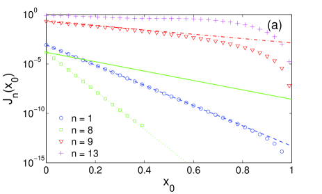
Figure 4: (Color online) The squared L2subscript𝐿2L_{2}-norm, Jn(x0)subscript𝐽𝑛subscript𝑥0J_{n}(x_{0}), of four eigenfunctions with n=1,8,9,13𝑛18913n=1,8,9,13 (symbols) for the rectangular branch on Fig. 2a. The estimate (31) with μ=π2/(1/4)2𝜇superscript𝜋2superscript142\mu=\pi^{2}/(1/4)^{2} is plotted by dashed (n=1𝑛1n=1), solid (n=8𝑛8n=8) and dash-dotted (n=9𝑛9n=9) lines. The estimate with μ=π2/(1/8)2𝜇superscript𝜋2superscript182\mu=\pi^{2}/(1/8)^{2} is shown for n=8𝑛8n=8 by dotted line.

Rectangular branch

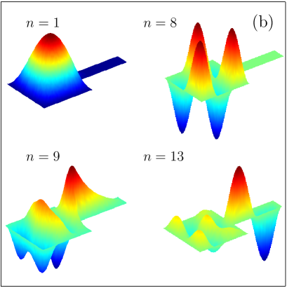
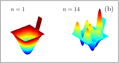
We start with a rectangular branch of width b=1/4𝑏14b=1/4 (Fig. 2a), for which μ=π2/(1/4)2157.91𝜇superscript𝜋2superscript142similar-to-or-equals157.91\mu=\pi^{2}/(1/4)^{2}\simeq 157.91..., and there are 9 eigenvalues λnsubscript𝜆𝑛\lambda_{n} below μ𝜇\mu (the first 20 eigenvalues are listed in Table 1). Figure 4a shows Jn(x0)subscript𝐽𝑛subscript𝑥0J_{n}(x_{0}) for four eigenfunctions with n=1,8,9,13𝑛18913n=1,8,9,13. These four eigenfunctions are chosen to illustrate different possibilities. For the eigenmodes with n=1,2,5,7,9𝑛12579n=1,2,5,7,9 (illustrated by n=1,9𝑛19n=1,9), the estimate is very accurate. In this case, the decay rate 2γn2subscript𝛾𝑛2\gamma_{n} is sharp and cannot be improved. There is another group of eigenfunctions with n=3,4,6,8𝑛3468n=3,4,6,8 (illustrated by n=8𝑛8n=8), for which Jn(x0)subscript𝐽𝑛subscript𝑥0J_{n}(x_{0}) is significantly smaller than the estimate. For x0<0.4subscript𝑥00.4x_{0}<0.4, J8(x0)subscript𝐽8subscript𝑥0J_{8}(x_{0}) decays as J8(0)exp[2γ8x0]subscript𝐽802subscriptsuperscript𝛾8subscript𝑥0J_{8}(0)\exp[-2\gamma^{\prime}_{8}x_{0}], where 2γ8=24μλ82subscriptsuperscript𝛾824𝜇subscript𝜆82\gamma^{\prime}_{8}=2\sqrt{4\mu-\lambda_{8}} is the improved decay rate (for larger x0subscript𝑥0x_{0}, the computation is inaccurate as explained earlier and its result is not shown). In order to understand this behavior, one can inspect the shape of the eigenfunction u8(x,y)subscript𝑢8𝑥𝑦u_{8}(x,y) shown on Fig. 4b. This function is anti-symmetric with respect to the horizontal line which splits the domain D𝐷D into two symmetric subdomains. As a consequence, u8(x,y)subscript𝑢8𝑥𝑦u_{8}(x,y) is 00 along this line and it is thus a solution of the Dirichlet eigenvalue problem for each subdomain (Fig. 2b). The width of the branch in each subdomain is twice smaller so that one can apply the general estimate with μ=4μsuperscript𝜇4𝜇\mu^{\prime}=4\mu. This is a special feature of all symmetric domains.

If the branch was shifted upwards or downwards, the reflection symmetry would be broken, and the decay rate 2γn2superscriptsubscript𝛾𝑛2\gamma_{n}^{\prime} would not be applicable any more. However, if the shift is small, one may still expect a faster exponential decrease with the decay rate between 2γn2subscript𝛾𝑛2\gamma_{n} and 2γn2superscriptsubscript𝛾𝑛2\gamma_{n}^{\prime}. This example shows that the estimate (13) may not be sharp for certain eigenfunctions. At the same time, it cannot be improved in general, as illustrated by the eigenfunctions with n=1,9𝑛19n=1,9.

The last curve shown on Fig. 4a by pluses, corresponds to n=13𝑛13n=13, for which λ13>μsubscript𝜆13𝜇\lambda_{13}>\mu, and the exponentially decaying estimate is not applicable. One can see that the function J13(x0)subscript𝐽13subscript𝑥0J_{13}(x_{0}) slowly varies along the branch. This behavior is also expected from its shape shown on Fig. 4b.

Narrow/wide and wide/narrow branches

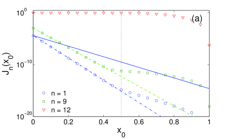
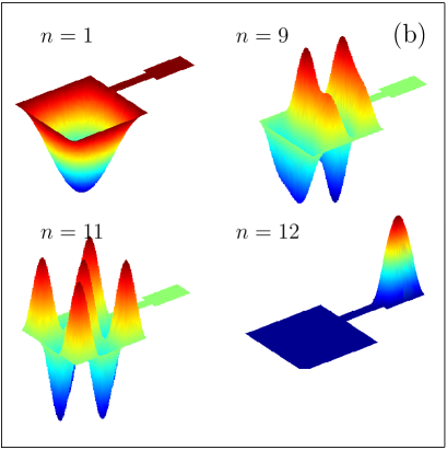
In two dimensions, any cross-section Ω(x)Ω𝑥\Omega(x) of a branch is a union of intervals. If (x)𝑥\ell(x) is the length of the largest interval in Ω(x)Ω𝑥\Omega(x) then the first eigenvalue μ(x)𝜇𝑥\mu(x) in Ω(x)Ω𝑥\Omega(x) is simply π2/(x)2superscript𝜋2superscript𝑥2\pi^{2}/\ell(x)^{2}. Whatever the shape of the branch is, the bound μ𝜇\mu for the exponential decay is then set by the length of the largest cross-section b=max0<x<a(x)𝑏subscript0𝑥𝑎𝑥b=\max\limits_{0<x<a}\ell(x) according to μ=π2/b2𝜇superscript𝜋2superscript𝑏2\mu=\pi^{2}/b^{2}. At first thought, this statement can sound counter-intuitive because one could expect that the asymptotic behavior would be determined by the smallest cross-section. In order to clarify this point, we consider an example on Fig. 2c for which μ=π2/(1/4)2𝜇superscript𝜋2superscript142\mu=\pi^{2}/(1/4)^{2}. Although the narrow channel of width b/2𝑏2b/2 strongly attenuates the amplitude of the eigenfunction, it does not imply the exponential decay with a hypothetical rate 24μλ24𝜇𝜆2\sqrt{4\mu-\lambda} along the next wider channel (Fig. 5). For instance, the function J1(x0)subscript𝐽1subscript𝑥0J_{1}(x_{0}) exponentially decays with the rate 24μλ24𝜇𝜆2\sqrt{4\mu-\lambda} (dashed line) up to x00.45subscript𝑥00.45x_{0}\approx 0.45. However, this decay is slowed down for x0.45𝑥0.45x\geq 0.45. The theoretical estimate with the decay rate 2μλ2𝜇𝜆2\sqrt{\mu-\lambda} (solid line) is of course applicable for all x0subscript𝑥0x_{0} but it is not sharp.

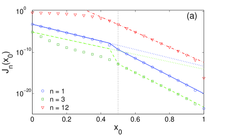
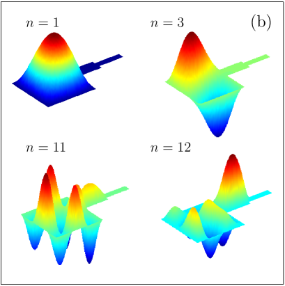
If the wide channel is placed first (as shown on Fig. 2d), the situation is different. The decay rate 2μλ2𝜇𝜆2\sqrt{\mu-\lambda}, which is set by the largest cross-section length b=1/4𝑏14b=1/4, can be used in the wide part of the branch. Although this result is also applicable in the narrow part, the estimate here can be improved. In fact, if one considers the unit square and the wide branch as a basic domain, the decay rate for the narrow branch, 24μλ24𝜇𝜆2\sqrt{4\mu-\lambda}, is the set by its width b/2=1/8𝑏218b/2=1/8 (Fig. 6). More generally, if the branch is a union of several branches with progressively decreasing widths, one can combine the exponential estimates with progressively increasing decay rates.
Refer to caption
Refer to caption
Figure 5: (Color online) The squared L2subscript𝐿2L_{2}-norm, Jn(x0)subscript𝐽𝑛subscript𝑥0J_{n}(x_{0}), of three eigenfunctions with n=1,9,12𝑛1912n=1,9,12 (symbols) for the narrow-than-wide branch on Fig. 2c. The estimate (31) with μ=π2/(1/4)2𝜇superscript𝜋2superscript142\mu=\pi^{2}/(1/4)^{2} is plotted for n=1𝑛1n=1 by solid line. The hypothetical estimate with μ=π2/(1/8)2𝜇superscript𝜋2superscript182\mu=\pi^{2}/(1/8)^{2} is shown by dash-dotted (n=1𝑛1n=1) and dashed (n=9𝑛9n=9) lines. The vertical dotted line indicates the connection between two parts of the branch.
Refer to caption
Refer to caption
Figure 6: (Color online) The squared L2subscript𝐿2L_{2}-norm, Jn(x0)subscript𝐽𝑛subscript𝑥0J_{n}(x_{0}), of three eigenfunctions with n=1,3,12𝑛1312n=1,3,12 (symbols) for the wide-than-narrow branch on Fig. 2d. The estimate (31) with μ=π2/(1/4)2𝜇superscript𝜋2superscript142\mu=\pi^{2}/(1/4)^{2} is plotted by dotted lines for n=1𝑛1n=1 and n=3𝑛3n=3. The combined estimate (for the wide part with μ=π2/(1/4)2𝜇superscript𝜋2superscript142\mu=\pi^{2}/(1/4)^{2} and for the narrow part with μ=π2/(1/8)2𝜇superscript𝜋2superscript182\mu=\pi^{2}/(1/8)^{2}) is shown by solid (n=1𝑛1n=1), dashed (n=3𝑛3n=3) and dash-dotted (n=12𝑛12n=12) lines. The vertical dotted line indicates the connection between two parts of the branch.

Increasing branch

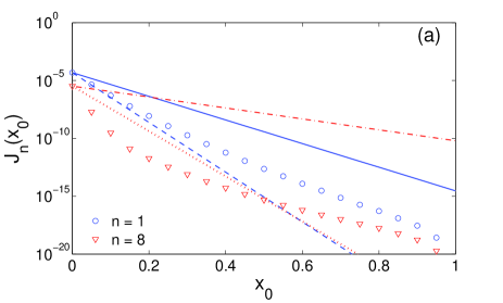
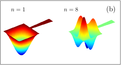
In the previous example on Fig. 2c, the supplementary condition (15) was not satisfied on a part of the branch boundary. Nevertheless, the numerical computation confirmed the sharp decay rate (16). In order to check the relevance of the condition (15), we consider a linearly increasing branch shown on Fig. 2e. Although the condition (15) is not satisfied at any point, the sharp decay rate (16) is again applicable, as shown on Fig. 7. In a future work, one may try to relax the condition (15) or to provide counter-examples showing its relevance.
Refer to caption
Refer to caption
Figure 7: The squared L2subscript𝐿2L_{2}-norm, Jn(x0)subscript𝐽𝑛subscript𝑥0J_{n}(x_{0}), of two eigenfunctions with n=1,8𝑛18n=1,8 (symbols) for the increasing branch on Fig. 2e. The estimate (31) with μ=π2/(1/4)2𝜇superscript𝜋2superscript142\mu=\pi^{2}/(1/4)^{2} is plotted by solid (n=1𝑛1n=1) and dash-dotted (n=8𝑛8n=8) lines. The hypothetical estimate with μ=π2/(1/8)2𝜇superscript𝜋2superscript182\mu=\pi^{2}/(1/8)^{2} is shown by dashed (n=1𝑛1n=1) and dotted (n=8𝑛8n=8) lines.

Branch with a cut

A small variation in the shape of the domain is known to result in small changes in eigenvalues of the Laplace operator, at least at the beginning of the spectrum (see Table 1). In turn, the eigenfunctions may be very sensitive to any perturbation of the domain. Bearing this sensitivity in mind, one can check the robustness of the exponential decay. We consider a horizontal cut at the middle of the rectangular branch (Fig. 2f). If the cut went along the whole branch, it would be equivalent to two separate rectangular branches of width b/2𝑏2b/2. In this case, the theoretical estimate could be applied individually to each branch, and the value μ=π2/(b/2)2𝜇superscript𝜋2superscript𝑏22\mu=\pi^{2}/(b/2)^{2} would be 4 times larger than for the original rectangular branch of width b𝑏b. For a partial cut, whatever its length is, the theoretical decay rate is again determined by μ=π2/(1/4)2𝜇superscript𝜋2superscript142\mu=\pi^{2}/(1/4)^{2} as for the rectangular branch. At the same time, it is clear that the cut results in a stronger “expelling” of eigenfunctions from the branch.

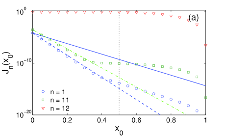
Figure 8a shows the squared L2subscript𝐿2L_{2}-norm, Jn(x0)subscript𝐽𝑛subscript𝑥0J_{n}(x_{0}), of three eigenfunctions with n=1,11,12𝑛11112n=1,11,12. For the first eigenfunction, we plot two exponential estimates, one with the rigorous value μ=π2/(1/4)2𝜇superscript𝜋2superscript142\mu=\pi^{2}/(1/4)^{2} and the other with a hypothetical value μ=π2/(1/8)2=4μsuperscript𝜇superscript𝜋2superscript1824𝜇\mu^{\prime}=\pi^{2}/(1/8)^{2}=4\mu for a twice narrower branch (if the cut was complete). Although the first estimate is of course applicable for the whole region, it is not sharp. In turn, the second estimate is sharp but it works only up to x0<0.4subscript𝑥00.4x_{0}<0.4. One can see that for x0>0.4subscript𝑥00.4x_{0}>0.4, the slope of lnJ1(x0)subscript𝐽1subscript𝑥0\ln J_{1}(x_{0}) is given by the first estimate. The best estimate would be a combination of these two but its construction depends on the specific shape of the branch. It is worth noting that the transition between two estimates (i.e., the point 0.40.40.4) does not appear at the end of the cut (here, at 0.50.50.5). This means that one cannot consider two subregions (with and without cut) separately in order to develop the individual estimates.

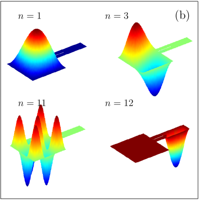
The 11th eigenvalue λ11177.0subscript𝜆11177.0\lambda_{11}\approx 177.0 exceeds μ𝜇\mu so that the rigorous decay rate is not applicable. In turn, the use of the hypothetical value μsuperscript𝜇\mu^{\prime} provides a good estimate up to x0<0.3subscript𝑥00.3x_{0}<0.3 but fails for x0>0.3subscript𝑥00.3x_{0}>0.3. Finally, the 12th eigenfunction has no exponential decay (in fact, it is localized in the branch).
Refer to caption
Refer to caption
Figure 8: (Color online) The squared L2subscript𝐿2L_{2}-norm, Jn(x0)subscript𝐽𝑛subscript𝑥0J_{n}(x_{0}), of three eigenfunctions with n=1,11,12𝑛11112n=1,11,12 (symbols) for the branch with a cut on Fig. 2f. The estimate (31) with μ=π2/(1/4)2𝜇superscript𝜋2superscript142\mu=\pi^{2}/(1/4)^{2} is plotted by solid (n=1𝑛1n=1) and dash-dotted (n=11𝑛11n=11) lines. The hypothetical estimate with μ=π2/(1/8)2𝜇superscript𝜋2superscript182\mu=\pi^{2}/(1/8)^{2} for n=1𝑛1n=1 is shown by dashed line. The vertical dotted line indicates the end of the cut.

Tilted and circular branches

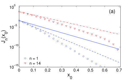
Another interesting question is the parameterization of the branch Q𝑄Q. In Sec. 3, a variable shape of the branch was implemented through the cross-section profile Ω(x)Ω𝑥\Omega(x) where x𝑥x ranged from 00 and a𝑎a. The choice of the x𝑥x coordinate is conventional and any other coordinate axis could be used instead of x𝑥x (by rotating the domain). However, the freedom of rotation may lead to inaccurate estimate for the decay rate. This point is illustrated by the domain on Fig. 2g with a rectangular branch tilted by 45superscript4545^{\circ}. Applying formally the estimate (13), one expects the exponential decay with μ=π2/(1/4)2157.91𝜇superscript𝜋2superscript142157.91\mu=\pi^{2}/(1/4)^{2}\approx 157.91. At the same time, if the whole domain was turned clockwise by 45superscript4545^{\circ} [or, equivalently, if the branch was parameterized along the axis xsuperscript𝑥x^{\prime} in the direction (1,1)11(1,1)], the decay rate would be set by μ=π2/(1/4/2)2315.83𝜇superscript𝜋2superscript1422315.83\mu=\pi^{2}/(1/4/\sqrt{2})^{2}\approx 315.83. It is clear that the behavior of eigenfunctions does not depend neither on rotations of the domain, nor on the parameterization of the branch. Figure 9 confirms the exponential decay with the latter threshold μ𝜇\mu.

Refer to caption
Refer to caption
Figure 9: (Color online) The squared L2subscript𝐿2L_{2}-norm, Jn(x0)subscript𝐽𝑛subscript𝑥0J_{n}(x_{0}), of two eigenfunctions with n=1,14𝑛114n=1,14 (symbols) for the tilted branch on Fig. 2g. The formal estimate (31) with μ=π2/(1/4)2𝜇superscript𝜋2superscript142\mu=\pi^{2}/(1/4)^{2} is plotted by solid line for n=1𝑛1n=1. The improved estimate with μ=π2/(1/4/2))2\mu=\pi^{2}/(1/4/\sqrt{2}))^{2} is shown by dashed (n=1𝑛1n=1) and dash-dotted (n=14𝑛14n=14) lines.

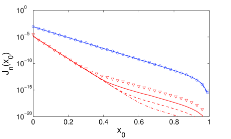
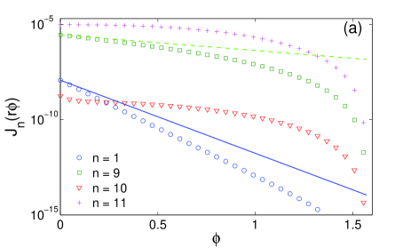
A circular branch on Fig. 2h is another example, for which the choice of parameterization is important. Using the “conventional” parameterization by the x𝑥x coordinate, the largest cross-section appears at x=3/8𝑥38x=3/8, and it is equal to 1/2121/2 so that μ=π2/(1/2)239.48𝜇superscript𝜋2superscript12239.48\mu=\pi^{2}/(1/2)^{2}\approx 39.48. Only the first eigenvalue λ1subscript𝜆1\lambda_{1} is below μ𝜇\mu so that the exponential estimate is not formally applicable to other eigenfunctions. At the same time, it is clear that the circular branch of “true” width b𝑏b can be naturally parameterized by the angle ϕitalic-ϕ\phi or, equivalently, by an arc, as illustrated on Fig. 2h. However, there is an ambiguity in the choice between arcs of various radii (e.g., inner, outer or middle arcs). Although the length of all these arcs is proportional to the angle ϕitalic-ϕ\phi, the proportionality coefficient enters in the decay rate. For the results plotted on Fig. 10, the inner arc of radius r=3/8𝑟38r=3/8 was used. The squared L2subscript𝐿2L_{2}-norm was plotted as a function of the curvilinear coordinate x0=rϕsuperscriptsubscript𝑥0𝑟italic-ϕx_{0}^{\prime}=r\phi, with ϕitalic-ϕ\phi varying between 00 and π/2𝜋2\pi/2. For such a curvilinear parameterization, the width of the branch is constant, b=1/4𝑏14b=1/4, so that there are 9 eigenvalues λnsubscript𝜆𝑛\lambda_{n} below μ=π2/(1/4)2𝜇superscript𝜋2superscript142\mu=\pi^{2}/(1/4)^{2}. For instance, the exponential decay of the 9th eigenfunction is confirmed on Fig. 10. For circular branches, rigorous estimates can be derived by writing explicit series representations of eigenfunctions in a circular annulus and reformulating the analysis similar to that of Sec. 2 (this analysis is beyond the scope of the paper). In general, an extension of the derivation in Sec. 3 to curvilinear parameterizations is an interesting perspective.
Refer to caption
Refer to caption
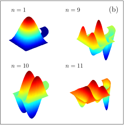
Figure 10: The squared L2subscript𝐿2L_{2}-norm, Jn(x0)subscript𝐽𝑛subscriptsuperscript𝑥0J_{n}(x^{\prime}_{0}), of four eigenfunctions with n=1,9,10,11𝑛191011n=1,9,10,11 (symbols) for the circular branch on Fig. 2h. The estimate (31) with μ=π2/(1/4)2𝜇superscript𝜋2superscript142\mu=\pi^{2}/(1/4)^{2} is plotted by solid (n=1𝑛1n=1) and dashed (n=9𝑛9n=9) lines. The curvilinear coordinate x0=rϕsuperscriptsubscript𝑥0𝑟italic-ϕx_{0}^{\prime}=r\phi with r=3/8𝑟38r=3/8 and the angle ϕitalic-ϕ\phi varying from 00 to π/2𝜋2\pi/2, was used.

Branch with a small broadening

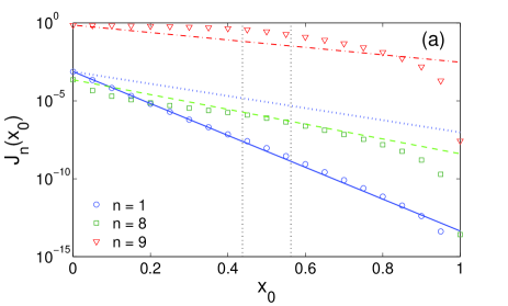
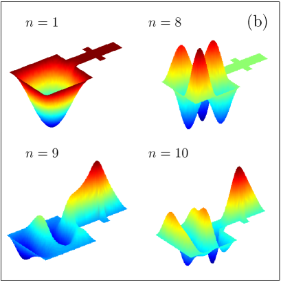
A small broadening in the middle is another interesting perturbation of the rectangular branch (Fig. 2i). Although this perturbation is small, the threshold value is reduced to μ=π2/(1/2)239.48𝜇superscript𝜋2superscript12239.48\mu=\pi^{2}/(1/2)^{2}\approx 39.48, instead of the value μ=π2/(1/4)2157.91superscript𝜇superscript𝜋2superscript142157.91\mu^{\prime}=\pi^{2}/(1/4)^{2}\approx 157.91 for the rectangular branch. As a consequence, the sufficient condition λn<μsubscript𝜆𝑛𝜇\lambda_{n}<\mu is satisfied only for n=1𝑛1n=1, while for other n𝑛n, the exponential estimate (13) cannot be applied. One may thus wonder how do these eigenfunctions behave in the branch?

We checked that the 8 first eigenfunctions exponentially decay along the branch, similarly to the rectangular case. In turn, the 9th, 10th and some other eigenfunctions do not exhibit this behavior. Figure 11 illustrates this result for three eigenfunctions with n=1,8,9𝑛189n=1,8,9. Since the rigorous estimate is not applicable, we plot the function Jn(0)exp(2μλnx0)subscript𝐽𝑛02superscript𝜇subscript𝜆𝑛subscript𝑥0J_{n}(0)\exp(-2\sqrt{\mu^{\prime}-\lambda_{n}}x_{0}) with μ=π2/(1/4)2superscript𝜇superscript𝜋2superscript142\mu^{\prime}=\pi^{2}/(1/4)^{2} as for the rectangular branch. One can see that this function correctly captures the behavior of Jn(x0)subscript𝐽𝑛subscript𝑥0J_{n}(x_{0}) but fails to be its upper bound (there are some regions in which Jn(x0)subscript𝐽𝑛subscript𝑥0J_{n}(x_{0}) exceeds this function).

In summary, in spite of the fact that the condition λ<μ𝜆𝜇\lambda<\mu is not satisfied, the presence of a small broadening does not significantly affect the exponential decay of the first eigenfunctions but the upper bound is not valid.
Refer to caption
Refer to caption
Figure 11: (Color online) The squared L2subscript𝐿2L_{2}-norm, Jn(x0)subscript𝐽𝑛subscript𝑥0J_{n}(x_{0}), of three eigenfunctions with n=1,8,9𝑛189n=1,8,9 (symbols) for the branch with a broadening on Fig. 2i. The estimate (31) with μ=π2/(1/2)2𝜇superscript𝜋2superscript122\mu=\pi^{2}/(1/2)^{2} for n=1𝑛1n=1 is shown by dotted line. The hypothetical estimate (31) with μ=π2/(1/4)2𝜇superscript𝜋2superscript142\mu=\pi^{2}/(1/4)^{2} is plotted by solid (n=1𝑛1n=1), dashed (n=8𝑛8n=8) and dash-dotted (n=9𝑛9n=9) lines. Vertical dotted lines indicate the position of the broadening.

Bifurcating branch

After describing the eigenfunctions in a single branch, one may wonder about their properties in a general pore network which consists of basic domains (“pores”) connected by branches. In spite of numerous potential applications for diffusive transport in porous media, very little is known about this challenging problem. A dumbbell domain with a thin “handle” is probably the most studied case [26, 27, 28, 29]. In particular, the method of matching asymptotic series yields the asymptotic estimates when the diameter of the channel is considered as a small parameter.

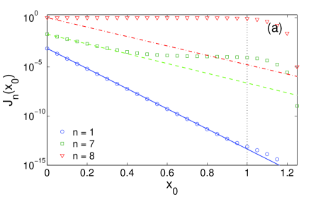
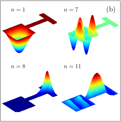
In order to illustrate the related difficulties, we consider a rectangular branch which bifurcates into two rectangular branches (Fig. 2j). For this example, the largest cross-section length is 111 so that μ=π29.87𝜇superscript𝜋29.87\mu=\pi^{2}\approx 9.87 and the exponential estimate is not applicable. Figure 12 shows Jn(x0)subscript𝐽𝑛subscript𝑥0J_{n}(x_{0}) for three eigenfunctions with n=1,7,8𝑛178n=1,7,8 and the hypothetical estimate with μ=π2/(1/4)2superscript𝜇superscript𝜋2superscript142\mu^{\prime}=\pi^{2}/(1/4)^{2} as for the rectangular branch. The first eigenfunction is well estimated by the exponential function J1(0)exp(2μλ1x0)subscript𝐽102superscript𝜇subscript𝜆1subscript𝑥0J_{1}(0)\exp(-2\sqrt{\mu^{\prime}-\lambda_{1}}x_{0}) for practically the whole length of the branch (x0<1subscript𝑥01x_{0}<1), with a small deviation at the bifurcation region (x0>1subscript𝑥01x_{0}>1). Similar behavior is observed for other eigenfunctions up to n=7𝑛7n=7. The larger the index n𝑛n, the earlier the deviation from the exponential estimate appears (e.g., for n=7𝑛7n=7, the estimate works only for x0<0.3subscript𝑥00.3x_{0}<0.3). In turn, the 8th eigenfunction has no exponential decay in the branch as it is localized in the bifurcation region. At the same time, the corresponding eigenvalues are close: λ7125.20subscript𝜆7125.20\lambda_{7}\approx 125.20 and λ8127.67subscript𝜆8127.67\lambda_{8}\approx 127.67. This illustrates how significant may be the difference in properties of two consecutive eigenfunctions. We also emphasize on the difficulty of distinguishing these cases in general.
Refer to caption
Refer to caption
Figure 12: (Color online) The squared L2subscript𝐿2L_{2}-norm, Jn(x0)subscript𝐽𝑛subscript𝑥0J_{n}(x_{0}), of three eigenfunctions with n=1,7,8𝑛178n=1,7,8 (symbols) for the bifurcating branch on Fig. 2j. The hypothetical estimate (31) with μ=π2/(1/4)2𝜇superscript𝜋2superscript142\mu=\pi^{2}/(1/4)^{2} is plotted by solid (n=1𝑛1n=1), dashed (n=7𝑛7n=7) and dash-dotted (n=8𝑛8n=8) lines. The vertical dotted line indicates the position of bifurcation.

Surprisingly, an exponential decay can be recovered for thinner bifurcations of arbitrary length. Although this example may look specific, the arguments provided below are of general interest. In order to prove the exponential decay of the squared norm J(x0)𝐽subscript𝑥0J(x_{0}) in Eq. (29), we will establish the inequalities similar to those for I(x0)𝐼subscript𝑥0I(x_{0}) of Sec. 3. Replacing the norm I(x0)𝐼subscript𝑥0I(x_{0}) by the weaker norm J(x0)𝐽subscript𝑥0J(x_{0}) allows one to produce more accurate estimates. Although we bear in mind the example shown on Fig. 2j, the arguments are rather general and applicable in higher dimensions. By definition, one has

J(x0)=I(x0)=Ω(x0)u2(x0,𝐲)𝑑𝐲<0superscript𝐽subscript𝑥0𝐼subscript𝑥0subscriptΩsubscript𝑥0superscript𝑢2subscript𝑥0𝐲differential-d𝐲0J^{\prime}(x_{0})=-I(x_{0})=-\int\limits_{\Omega(x_{0})}u^{2}(x_{0},{\bf y})d{\bf y}<0

and

J′′(x0)=2Ω(x0)uxu𝑑𝐲=2Q(x0)[(u,u)+uΔu]𝑑x𝑑𝐲,superscript𝐽′′subscript𝑥02subscriptΩsubscript𝑥0𝑢𝑥𝑢differential-d𝐲2subscript𝑄subscript𝑥0delimited-[]𝑢𝑢𝑢Δ𝑢differential-d𝑥differential-d𝐲\begin{split}J^{\prime\prime}(x_{0})&=-2\int\limits_{\Omega(x_{0})}u\frac{\partial}{\partial x}ud{\bf y}=2\int\limits_{Q(x_{0})}\bigl{[}(\nabla u,\nabla u)+u\Delta u\bigr{]}dxd{\bf y},\\ \end{split}

where the Green’s formula, the identity /x=/n𝑥𝑛\partial/\partial x=-\partial/\partial n on Ω(x0)Ωsubscript𝑥0\Omega(x_{0}) and Dirichlet boundary condition on Q(x0)\Ω(x0)\𝑄subscript𝑥0Ωsubscript𝑥0\partial Q(x_{0})\backslash\Omega(x_{0}) were used. The first integral can be estimated by splitting Q(x0)𝑄subscript𝑥0Q(x_{0}) into two subdomains: Q1(x0)subscript𝑄1subscript𝑥0Q_{1}(x_{0}) (a part of the rectangular branch) and Q2subscript𝑄2Q_{2} (the bifurcation):

Q(x0)(u,u)𝑑x𝑑𝐲μQ1(x0)u2𝑑x𝑑𝐲+Q2(u,u)𝑑x𝑑𝐲,subscript𝑄subscript𝑥0𝑢𝑢differential-d𝑥differential-d𝐲𝜇subscriptsubscript𝑄1subscript𝑥0superscript𝑢2differential-d𝑥differential-d𝐲subscriptsubscript𝑄2𝑢𝑢differential-d𝑥differential-d𝐲\int\limits_{Q(x_{0})}(\nabla u,\nabla u)dxd{\bf y}\geq\mu\int\limits_{Q_{1}(x_{0})}u^{2}dxd{\bf y}+\int\limits_{Q_{2}}(\nabla u,\nabla u)dxd{\bf y},

where the Friedrichs-Poincaré inequality was used for Q1(x0)subscript𝑄1subscript𝑥0Q_{1}(x_{0}), with the smallest μ𝜇\mu over Q1(x0)subscript𝑄1subscript𝑥0Q_{1}(x_{0}) (for the rectangular branch on Fig. 2j, μ=π2/b2𝜇superscript𝜋2superscript𝑏2\mu=\pi^{2}/b^{2}). The separate analysis of two subdomains allowed us to exclude large cross-sections of the bifurcation Q2subscript𝑄2Q_{2} from the computation of μ𝜇\mu.

In order to estimate the second integral over Q2subscript𝑄2Q_{2}, we note that

ν1=infvH1(Q2),v|Γ=0,v0(v,v)(v,v)subscript𝜈1subscriptinfimumformulae-sequence𝑣superscript𝐻1subscript𝑄2formulae-sequenceevaluated-at𝑣Γ0𝑣0𝑣𝑣𝑣𝑣\nu_{1}=\inf\limits_{v\in H^{1}(Q_{2}),~{}v|_{\Gamma}=0,~{}v\neq 0}\frac{(\nabla v,\nabla v)}{(v,v)}

is the smallest eigenvalue of the Laplace operator in the rectangle Q2subscript𝑄2Q_{2} with Dirichlet boundary condition on the top, bottom and right segments (denoted by ΓΓ\Gamma) and Neumann boundary condition on the left segment. Since the eigenfunction u𝑢u also belongs to H1(Q2)superscript𝐻1subscript𝑄2H^{1}(Q_{2}), one has

(u,u)L2(Q2)ν1(u,u)L2(Q2),subscript𝑢𝑢subscript𝐿2subscript𝑄2subscript𝜈1subscript𝑢𝑢subscript𝐿2subscript𝑄2(\nabla u,\nabla u)_{L_{2}(Q_{2})}\geq\nu_{1}(u,u)_{L_{2}(Q_{2})},

from which

J′′(x0)2(μλ)Q1(x0)u2𝑑x𝑑𝐲+2(ν1λ)Q2u2𝑑x𝑑𝐲.superscript𝐽′′subscript𝑥02𝜇𝜆subscriptsubscript𝑄1subscript𝑥0superscript𝑢2differential-d𝑥differential-d𝐲2subscript𝜈1𝜆subscriptsubscript𝑄2superscript𝑢2differential-d𝑥differential-d𝐲J^{\prime\prime}(x_{0})\geq 2(\mu-\lambda)\int\limits_{Q_{1}(x_{0})}u^{2}dxd{\bf y}+2(\nu_{1}-\lambda)\int\limits_{Q_{2}}u^{2}dxd{\bf y}.

If ν1>μsubscript𝜈1𝜇\nu_{1}>\mu, we finally obtain

J′′(x0)2(μλ)Q(x0)u2𝑑x𝑑𝐲=2(μλ)J(x0).superscript𝐽′′subscript𝑥02𝜇𝜆subscript𝑄subscript𝑥0superscript𝑢2differential-d𝑥differential-d𝐲2𝜇𝜆𝐽subscript𝑥0J^{\prime\prime}(x_{0})\geq 2(\mu-\lambda)\int\limits_{Q(x_{0})}u^{2}dxd{\bf y}=2(\mu-\lambda)J(x_{0}).

As shown in Sec. 3, this inequality implies an exponential decay of J(x0)𝐽subscript𝑥0J(x_{0}).

If Q2subscript𝑄2Q_{2} is a rectangle of height hh and width w𝑤w with Dirichlet boundary condition on the top, bottom and right segments and Neumann boundary condition on the left segment, the smallest eigenvalue is ν1=π2/h2+π2/(2w)2subscript𝜈1superscript𝜋2superscript2superscript𝜋2superscript2𝑤2\nu_{1}=\pi^{2}/h^{2}+\pi^{2}/(2w)^{2}. If the branch Q1subscript𝑄1Q_{1} is also a rectangle of width b𝑏b (as shown on Fig. 2j), one has μ=π2/b2𝜇superscript𝜋2superscript𝑏2\mu=\pi^{2}/b^{2}. The condition ν1>μsubscript𝜈1𝜇\nu_{1}>\mu reads as (b/h)2+(b/(2w))2>1superscript𝑏2superscript𝑏2𝑤21(b/h)^{2}+(b/(2w))^{2}>1. For instance, this condition is satisfied for any hh if the bifurcation width w𝑤w is smaller than b/2𝑏2b/2. In particular, this explains that a small broadening of width b/2𝑏2b/2 shown on Fig. 2i does not degrade the exponential decay of Jn(x0)subscript𝐽𝑛subscript𝑥0J_{n}(x_{0}) for x0<0.4375subscript𝑥00.4375x_{0}<0.4375. In turn, the bifurcation shown on Fig. 2j with h=11h=1 and w=b=1/4𝑤𝑏14w=b=1/4 does not fulfill the above condition as (b/h)2+(b/(2w))2=1/16+1/4<1superscript𝑏2superscript𝑏2𝑤2116141(b/h)^{2}+(b/(2w))^{2}=1/16+1/4<1.

4.2 Infinite branches

In the derivation of Sec. 3, there was no condition on the length a𝑎a of the branch. Even for an infinite branch, the exponential decay is valid once the condition (11) is satisfied. However, when the branch is infinite, the Laplace operator eigenspectrum is not necessarily discrete so that L2subscript𝐿2L_{2}-normalized eigenfunctions may not exist. A simple counter-example is a semi-infinite strip D=[0,)×[0,π]𝐷00𝜋D=[0,\infty)\times[0,\pi] for which functions sinh(n2λx)sin(ny)superscript𝑛2𝜆𝑥𝑛𝑦\sinh(\sqrt{n^{2}-\lambda}x)\sin(ny) satisfy the eigenvalue problem (8) but their L2(D)subscript𝐿2𝐷L_{2}(D) norms are infinite.

As shown by Rellich, if the first eigenvalue μ1(x)subscript𝜇1𝑥\mu_{1}(x) in the cross-section Ω(x)Ω𝑥\Omega(x) of an infinite branch Q𝑄Q goes to infinity as x𝑥x\to\infty, then there exist infinitely many L2subscript𝐿2L_{2}-normalized eigenfunctions [30]. In two dimensions, μ1(x)=π2/(x)2subscript𝜇1𝑥superscript𝜋2superscript𝑥2\mu_{1}(x)=\pi^{2}/\ell(x)^{2} is related to the length (x)𝑥\ell(x) of the largest interval in the cross-section Ω(x)Ω𝑥\Omega(x). The condition μ1(x)subscript𝜇1𝑥\mu_{1}(x)\to\infty requires thus (x)0𝑥0\ell(x)\to 0. At the same time, the number of intervals in Ω(x)Ω𝑥\Omega(x) can increase with x𝑥x so that the “total width” of the branch may arbitrarily increase.

For infinite decreasing branches, eigenfunctions can be shown to decay faster than an exponential with any decay rate. In fact, although the threshold μ𝜇\mu was defined in (10) as the smallest μ1(x)subscript𝜇1𝑥\mu_{1}(x) over all cross-sections of the branch, the separation into a basic domain and a branch was somewhat arbitrary. If the separation occurs at x0subscript𝑥0x_{0} (instead of 00), one gets

I(x)I(x0)exp[2μ(x0)λ(xx0)]xx0,formulae-sequence𝐼𝑥𝐼subscript𝑥02𝜇subscript𝑥0𝜆𝑥subscript𝑥0𝑥subscript𝑥0I(x)\leq I(x_{0})\exp[-2\sqrt{\mu(x_{0})-\lambda}~{}(x-x_{0})]\quad x\geq x_{0},

where the new threshold μ(x0)=infx0<xμ1(x)𝜇subscript𝑥0subscriptinfimumsubscript𝑥0𝑥subscript𝜇1𝑥\mu(x_{0})=\inf\limits_{x_{0}<x}\mu_{1}(x) increases with x0subscript𝑥0x_{0}, while the prefactor I(x0)𝐼subscript𝑥0I(x_{0}) also decays exponentially with x0subscript𝑥0x_{0} according to Eq. (13). Since the above estimate is applicable for any x0subscript𝑥0x_{0}, one can take x0subscript𝑥0x_{0} to be a slowly increasing function of x𝑥x [its choice depends on μ(x0)𝜇subscript𝑥0\mu(x_{0})] that would result in a faster-than-exponential decay of I(x)𝐼𝑥I(x). This result is a consequence of the condition μ1(x)subscript𝜇1𝑥\mu_{1}(x)\to\infty as x𝑥x goes to infinity.

4.3 Three-dimensional domains

The exponential estimate (13) becomes still more interesting in three (and higher) dimensions. While any cross-section Ω(x)Ω𝑥\Omega(x) was a union of intervals in two dimensions, the shape of cross-sections in three dimensions can vary significantly (e.g., see Fig. 1c). Whatever the shape of the branch is, the only relevant information for the exponential decay is the smallest eigenvalue μ𝜇\mu in all cross-sections Ω(x)Ω𝑥\Omega(x). For instance, for a rectangular profile of the branch, Ω(x)=[0,b(x)]×[0,c(x)]Ω𝑥0𝑏𝑥0𝑐𝑥\Omega(x)=[0,b(x)]\times[0,c(x)], the first eigenvalue μ1(x)=π2b(x)2+π2c(x)2subscript𝜇1𝑥superscript𝜋2𝑏superscript𝑥2superscript𝜋2𝑐superscript𝑥2\mu_{1}(x)=\frac{\pi^{2}}{b(x)^{2}}+\frac{\pi^{2}}{c(x)^{2}} can remain bounded from below by some μ𝜇\mu even if one of the sides b(x)𝑏𝑥b(x) or c(x)𝑐𝑥c(x) grows to infinity. This means that eigenfunctions may exponentially decay even in infinitely growing branches.

4.4 Neumann boundary condition

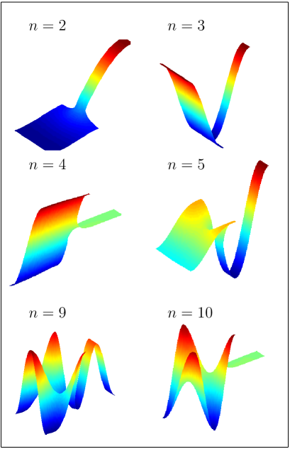
The theoretical derivation in Sec. 3 essentially relies on the Dirichlet boundary condition on the branch boundary: u|Q=0evaluated-at𝑢𝑄0u|_{\partial Q}=0. This condition can be interpreted, e.g., as a rigid fixation of a vibrating membrane at the boundary, or as a perfect absorption of diffusing particles at the boundary. The opposite case of free vibrations of the membrane or a perfect reflection of the particles is described by Neumann boundary condition, u/n|Q=0evaluated-at𝑢𝑛𝑄0\partial u/\partial n|_{\partial Q}=0. Although the eigenvalue problem may look similar, the behavior of eigenfunctions is different. In particular, an extension of the results of Sec. 3 fails even in the simplest case of a rectangular branch, as illustrated on Fig. 13. Although the 8 first eigenvalues λnsubscript𝜆𝑛\lambda_{n} are below μ=π2/(1/4)2𝜇superscript𝜋2superscript142\mu=\pi^{2}/(1/4)^{2}, only some of them decay exponentially (e.g., with n=4𝑛4n=4). This decay seems to be related to the reflection symmetry of the domain. Since the eigenfunctions with n=4,10𝑛410n=4,10 are anti-symmetric, they are 00 along the horizontal symmetry line. One can therefore split the domain into two symmetric subdomains and impose the Dirichlet boundary condition on the splitting line. Although an exponential decay may be expected for this new problem, its mathematical justification is beyond the scope of the paper.

On the other hand, the derivation of the exponential estimate in Sec. 3 does not use the boundary condition imposed on the basic domain V𝑉V. As a consequence, the estimate is applicable for arbitrary boundary condition on V𝑉V which guarantees the Laplace operator in the whole domain D𝐷D to be self-adjoint.

Refer to caption
Figure 13: Six eigenfunctions with n=2,3,4,5,9,10𝑛2345910n=2,3,4,5,9,10 for the rectangular branch (Fig. 2a) with Neumann boundary condition (the fundamental eigenfunction with n=1𝑛1n=1 is constant and not shown).

4.5 Expelling from the branch

It is important to stress that the “smallness” of an eigenfunction in the branch and its exponential decay are different notions which should not to be confused. In fact, the eigenfunction can be small in the branch either due to a rapid exponential decay, or because of the small constant In(0)subscript𝐼𝑛0I_{n}(0) or Jn(0)subscript𝐽𝑛0J_{n}(0) in front of the estimate. For instance, Fig. 10a shows the behavior of J10(x0)subscript𝐽10subscript𝑥0J_{10}(x_{0}) without an exponential decay, but the eigenfunction is nevertheless small (Fig. 10b). Another example on Fig. 4a with n=9𝑛9n=9 illustrates the opposite situation: the eigenfunction decays exponentially along the branch but it does not look small.

Conclusion

We have studied the behavior of the Laplace operator eigenfunctions in a large class of domains composed of a basic domain of arbitrary shape and a branch Q𝑄Q which can be parameterized by a variable profile Ω(x)Ω𝑥\Omega(x). We have rigorously proved that each eigenfunction whose eigenvalue λ𝜆\lambda is smaller than the threshold μ=inf{μ1(x)}𝜇infimumsubscript𝜇1𝑥\mu=\inf\{\mu_{1}(x)\}, exponentially decays inside the branch, where μ1(x)subscript𝜇1𝑥\mu_{1}(x) is the first eigenvalue of the Laplace operator in the cross-section Ω(x)Ω𝑥\Omega(x). In general, the decay rate was shown to be at least 2μλ2𝜇𝜆\sqrt{2}\sqrt{\mu-\lambda}. For non-increasing branches, the decay rate 2μλ2𝜇𝜆2\sqrt{\mu-\lambda} was derived and shown to be sharp for an appropriate parameterization of the branch. The exponential estimate is applicable in any dimension and for finite and infinite branches. In the latter case, the condition μ1(x)subscript𝜇1𝑥\mu_{1}(x)\to\infty as x𝑥x\to\infty is imposed to ensure the existence of L2subscript𝐿2L_{2}-normalized eigenfunctions. Since the derivation did not involve any information about the basic domain V𝑉V, the exponential estimate is applicable for arbitrary V𝑉V with any boundary condition on V𝑉\partial V for which the Laplace operator in D𝐷D is still self-adjoint. In turn, the Dirichlet boundary condition on the branch boundary was essential. Note that the mathematical methods of the paper can be adapted for studying eigenfunctions for various spectral problems or other types of domains.

The numerical simulations have been used to illustrate and extend the theoretical results. It was shown that the sufficient condition λ<μ𝜆𝜇\lambda<\mu is not necessary, i.e., the eigenfunctions may exponentially decay even if λ>μ𝜆𝜇\lambda>\mu. However, in this case, the decay rate and the range of its applicability strongly depend on the specific shape of the branch. For all numerical examples, the sharp decay rate 2μλ2𝜇𝜆2\sqrt{\mu-\lambda} was correct, even if the condition (15) for non-increasing branches was not satisfied. In future, it is tempting either to relax this condition, or to find counter-examples, for which the sharp decay is not applicable.

Acknowledgment

This work has been partly supported by the RFBR N 09-01-00408a grant and the ANR grant “SAMOVAR”.

Appendix A Estimate for rectangular branch

From the inequality sinhxcoshx𝑥𝑥\sinh x\leq\cosh x, Eq. (5) is bounded as

uL2(Q(x0))2b2n=1cn2[(πbn)2+γn2]x0acosh2(γn(ax))𝑑x.subscriptsuperscriptnorm𝑢2subscript𝐿2𝑄subscript𝑥0𝑏2superscriptsubscript𝑛1superscriptsubscript𝑐𝑛2delimited-[]superscript𝜋𝑏𝑛2superscriptsubscript𝛾𝑛2superscriptsubscriptsubscript𝑥0𝑎superscript2subscript𝛾𝑛𝑎𝑥differential-d𝑥||\nabla u||^{2}_{L_{2}(Q(x_{0}))}\leq\frac{b}{2}\sum\limits_{n=1}^{\infty}c_{n}^{2}\biggl{[}(\frac{\pi}{b}n)^{2}+\gamma_{n}^{2}\biggr{]}\int\limits_{x_{0}}^{a}\cosh^{2}(\gamma_{n}(a-x))dx.

The last integral is estimated as

x0acosh2(γn(ax))𝑑xx0ae2γn(ax)𝑑x=e2γna2γn(e2γnx0e2γna)e2γna2γne2γnx0e2γna2γne2γ1x0,superscriptsubscriptsubscript𝑥0𝑎superscript2subscript𝛾𝑛𝑎𝑥differential-d𝑥superscriptsubscriptsubscript𝑥0𝑎superscript𝑒2subscript𝛾𝑛𝑎𝑥differential-d𝑥superscript𝑒2subscript𝛾𝑛𝑎2subscript𝛾𝑛superscript𝑒2subscript𝛾𝑛subscript𝑥0superscript𝑒2subscript𝛾𝑛𝑎superscript𝑒2subscript𝛾𝑛𝑎2subscript𝛾𝑛superscript𝑒2subscript𝛾𝑛subscript𝑥0superscript𝑒2subscript𝛾𝑛𝑎2subscript𝛾𝑛superscript𝑒2subscript𝛾1subscript𝑥0\begin{split}&\int\limits_{x_{0}}^{a}\cosh^{2}(\gamma_{n}(a-x))dx\leq\int\limits_{x_{0}}^{a}e^{2\gamma_{n}(a-x)}dx=\\ &\frac{e^{2\gamma_{n}a}}{2\gamma_{n}}\bigl{(}e^{-2\gamma_{n}x_{0}}-e^{-2\gamma_{n}a}\bigr{)}\leq\frac{e^{2\gamma_{n}a}}{2\gamma_{n}}e^{-2\gamma_{n}x_{0}}\leq\frac{e^{2\gamma_{n}a}}{2\gamma_{n}}e^{-2\gamma_{1}x_{0}},\\ \end{split}

where we used the inequality coshxex𝑥superscript𝑒𝑥\cosh x\leq e^{x} for x0𝑥0x\geq 0 and the fact that γn=π2n2/b2λsubscript𝛾𝑛superscript𝜋2superscript𝑛2superscript𝑏2𝜆\gamma_{n}=\sqrt{\pi^{2}n^{2}/b^{2}-\lambda} increases with n𝑛n. We have then

uL2(Q(x0))2b2e2γ1x0n=1cn2[π2b2n22γn+γn2]e2γna.subscriptsuperscriptnorm𝑢2subscript𝐿2𝑄subscript𝑥0𝑏2superscript𝑒2subscript𝛾1subscript𝑥0superscriptsubscript𝑛1superscriptsubscript𝑐𝑛2delimited-[]superscript𝜋2superscript𝑏2superscript𝑛22subscript𝛾𝑛subscript𝛾𝑛2superscript𝑒2subscript𝛾𝑛𝑎||\nabla u||^{2}_{L_{2}(Q(x_{0}))}\leq\frac{b}{2}e^{-2\gamma_{1}x_{0}}\sum\limits_{n=1}^{\infty}c_{n}^{2}\biggl{[}\frac{\pi^{2}}{b^{2}}\frac{n^{2}}{2\gamma_{n}}+\frac{\gamma_{n}}{2}\biggr{]}e^{2\gamma_{n}a}.

Writing two inequalities:

γn=π2n2/b2λπbn,n2γn=n(π/b)1λb2/(π2n2)C1n,formulae-sequencesubscript𝛾𝑛superscript𝜋2superscript𝑛2superscript𝑏2𝜆𝜋𝑏𝑛superscript𝑛2subscript𝛾𝑛𝑛𝜋𝑏1𝜆superscript𝑏2superscript𝜋2superscript𝑛2subscript𝐶1𝑛\begin{split}\gamma_{n}&=\sqrt{\pi^{2}n^{2}/b^{2}-\lambda}\leq\frac{\pi}{b}n,\\ \frac{n^{2}}{\gamma_{n}}&=\frac{n}{(\pi/b)\sqrt{1-\lambda b^{2}/(\pi^{2}n^{2})}}\leq C_{1}n,\\ \end{split}

where C1subscript𝐶1C_{1} is a constant, one gets an upper bound in the order of n𝑛n for the expression in large brackets. Finally, we have an estimate for e2γnasuperscript𝑒2subscript𝛾𝑛𝑎e^{2\gamma_{n}a} as

sinh2(2γna)=e2γna4(1e2γna)2e2γna4(1e2γ1a)2,superscript22subscript𝛾𝑛𝑎superscript𝑒2subscript𝛾𝑛𝑎4superscript1superscript𝑒2subscript𝛾𝑛𝑎2superscript𝑒2subscript𝛾𝑛𝑎4superscript1superscript𝑒2subscript𝛾1𝑎2\sinh^{2}(2\gamma_{n}a)=\frac{e^{2\gamma_{n}a}}{4}(1-e^{-2\gamma_{n}a})^{2}\geq\frac{e^{2\gamma_{n}a}}{4}(1-e^{-2\gamma_{1}a})^{2},

from which

e2γnaC2sinh2(2γna),superscript𝑒2subscript𝛾𝑛𝑎subscript𝐶2superscript22subscript𝛾𝑛𝑎e^{2\gamma_{n}a}\leq C_{2}\sinh^{2}(2\gamma_{n}a),

with a constant C2=4/(1e2γ1a)2subscript𝐶24superscript1superscript𝑒2subscript𝛾1𝑎2C_{2}=4/(1-e^{-2\gamma_{1}a})^{2}. Bringing together these inequalities, we get the estimate (6).

Trace theorem

The trace theorem implies [31] that the series

f(x)n=1n(u(x,y),sin(πny/b))L2(0,b)2,𝑓𝑥superscriptsubscript𝑛1𝑛subscriptsuperscript𝑢𝑥𝑦𝜋𝑛𝑦𝑏2subscript𝐿20𝑏f(x)\equiv\sum\limits_{n=1}^{\infty}n\bigl{(}u(x,y),\sin(\pi ny/b)\bigr{)}^{2}_{L_{2}(0,b)},

which is equivalent to the squared norm of u(x,y)𝑢𝑥𝑦u(x,y) in the Sobolev space H(0,b)1/2superscriptsubscript𝐻0𝑏12H_{(0,b)}^{1/2}, may be estimated from above by the norm uL2(D)2subscriptsuperscriptnorm𝑢2subscript𝐿2𝐷||\nabla u||^{2}_{L_{2}(D)}. For completeness, we provide the proof for our special case.

For a fixed x𝑥x, we denote

Xn(x)(u(x,y),sin(πny/b))L2(0,b)subscript𝑋𝑛𝑥subscript𝑢𝑥𝑦𝜋𝑛𝑦𝑏subscript𝐿20𝑏X_{n}(x)\equiv\bigl{(}u(x,y),\sin(\pi ny/b)\bigr{)}_{L_{2}(0,b)}

the Fourier coefficients of the function u(x,y)𝑢𝑥𝑦u(x,y):

u(x,y)=2bn=1Xn(x)sin(πny/b).𝑢𝑥𝑦2𝑏superscriptsubscript𝑛1subscript𝑋𝑛𝑥𝜋𝑛𝑦𝑏u(x,y)=\frac{2}{b}\sum\limits_{n=1}^{\infty}X_{n}(x)\sin(\pi ny/b).

On one hand, starting from Xn(a)=0subscript𝑋𝑛𝑎0X_{n}(a)=0, one gets

Xn2(x)=|xa(Xn2)𝑑x1|=2|xaXnXn𝑑x1|,subscriptsuperscript𝑋2𝑛𝑥superscriptsubscript𝑥𝑎superscriptsubscriptsuperscript𝑋2𝑛differential-dsubscript𝑥12superscriptsubscript𝑥𝑎subscript𝑋𝑛subscriptsuperscript𝑋𝑛differential-dsubscript𝑥1X^{2}_{n}(x)=\left|\int\limits_{x}^{a}(X^{2}_{n})^{\prime}dx_{1}\right|=2\left|\int\limits_{x}^{a}X_{n}X^{\prime}_{n}dx_{1}\right|,

while the Cauchy inequality implies

2|xaXnXn𝑑x1|2XnL2(0,a)XnL2(0,a).2superscriptsubscript𝑥𝑎subscript𝑋𝑛subscriptsuperscript𝑋𝑛differential-dsubscript𝑥12subscriptnormsubscript𝑋𝑛subscript𝐿20𝑎subscriptnormsubscriptsuperscript𝑋𝑛subscript𝐿20𝑎2\left|\int\limits_{x}^{a}X_{n}X^{\prime}_{n}dx_{1}\right|\leq 2||X_{n}||_{L_{2}(0,a)}||X^{\prime}_{n}||_{L_{2}(0,a)}.

The inequality 2αβα2+β22𝛼𝛽superscript𝛼2superscript𝛽22\alpha\beta\leq\alpha^{2}+\beta^{2} yields

2(πn/b)XnL2(0,a)XnL2(0,a)XnL2(0,a)2+(πn/b)2XnL2(0,a)2,2𝜋𝑛𝑏subscriptnormsubscript𝑋𝑛subscript𝐿20𝑎subscriptnormsubscriptsuperscript𝑋𝑛subscript𝐿20𝑎subscriptsuperscriptnormsubscriptsuperscript𝑋𝑛2subscript𝐿20𝑎superscript𝜋𝑛𝑏2subscriptsuperscriptnormsubscript𝑋𝑛2subscript𝐿20𝑎\begin{split}2(\pi n/b)&||X_{n}||_{L_{2}(0,a)}||X^{\prime}_{n}||_{L_{2}(0,a)}\leq||X^{\prime}_{n}||^{2}_{L_{2}(0,a)}+(\pi n/b)^{2}||X_{n}||^{2}_{L_{2}(0,a)},\\ \end{split}

from which

(πn/b)Xn2(x)XnL2(0,a)2+(πn/b)2XnL2(0,a)2.𝜋𝑛𝑏subscriptsuperscript𝑋2𝑛𝑥subscriptsuperscriptnormsubscriptsuperscript𝑋𝑛2subscript𝐿20𝑎superscript𝜋𝑛𝑏2subscriptsuperscriptnormsubscript𝑋𝑛2subscript𝐿20𝑎(\pi n/b)X^{2}_{n}(x)\leq||X^{\prime}_{n}||^{2}_{L_{2}(0,a)}+(\pi n/b)^{2}||X_{n}||^{2}_{L_{2}(0,a)}.

On the other hand, we write explicitly the energetic norm of u𝑢u:

uL2(Q)2=2bn=1(XnL2(0,a)2+(πn/b)2XnL2(0,a)2),subscriptsuperscriptnorm𝑢2subscript𝐿2𝑄2𝑏superscriptsubscript𝑛1subscriptsuperscriptnormsubscriptsuperscript𝑋𝑛2subscript𝐿20𝑎superscript𝜋𝑛𝑏2subscriptsuperscriptnormsubscript𝑋𝑛2subscript𝐿20𝑎||\nabla u||^{2}_{L_{2}(Q)}=\frac{2}{b}\sum\limits_{n=1}^{\infty}\biggl{(}||X^{\prime}_{n}||^{2}_{L_{2}(0,a)}+(\pi n/b)^{2}||X_{n}||^{2}_{L_{2}(0,a)}\biggr{)},

from which

f(x)=n=1nXn2(x)b22πuL2(Q)2b22πuL2(D)2.𝑓𝑥superscriptsubscript𝑛1𝑛subscriptsuperscript𝑋2𝑛𝑥superscript𝑏22𝜋subscriptsuperscriptnorm𝑢2subscript𝐿2𝑄superscript𝑏22𝜋subscriptsuperscriptnorm𝑢2subscript𝐿2𝐷f(x)=\sum\limits_{n=1}^{\infty}nX^{2}_{n}(x)\leq\frac{b^{2}}{2\pi}||\nabla u||^{2}_{L_{2}(Q)}\leq\frac{b^{2}}{2\pi}||\nabla u||^{2}_{L_{2}(D)}.

Since the coefficients Xn(x)subscript𝑋𝑛𝑥X_{n}(x) and cnsubscript𝑐𝑛c_{n} are related as

Xn(x)=b2cnsinh(γn(ax)),subscript𝑋𝑛𝑥𝑏2subscript𝑐𝑛subscript𝛾𝑛𝑎𝑥X_{n}(x)=\frac{b}{2}~{}c_{n}\sinh(\gamma_{n}(a-x)),

the substitution of x=0𝑥0x=0 into this equation yields

n=1ncn2sinh2(γna)=4b2n=1nXn(0)2=4b2f(0)2λπuL2(D)2=2λπuL2(D)2.superscriptsubscript𝑛1𝑛superscriptsubscript𝑐𝑛2superscript2subscript𝛾𝑛𝑎4superscript𝑏2superscriptsubscript𝑛1𝑛subscript𝑋𝑛superscript024superscript𝑏2𝑓02𝜆𝜋subscriptsuperscriptnorm𝑢2subscript𝐿2𝐷2𝜆𝜋subscriptsuperscriptnorm𝑢2subscript𝐿2𝐷\begin{split}\sum\limits_{n=1}^{\infty}nc_{n}^{2}\sinh^{2}(\gamma_{n}a)&=\frac{4}{b^{2}}\sum\limits_{n=1}^{\infty}nX_{n}(0)^{2}=\frac{4}{b^{2}}f(0)\leq\frac{2\lambda}{\pi}||u||^{2}_{L_{2}(D)}=\frac{2\lambda}{\pi}||u||^{2}_{L_{2}(D)}.\\ \end{split} (32)

Appendix B Several classical results

For completeness, we recall the derivation of several classical results [31, 32] which are well known for spectral analysts but may be unfamiliar for other readers.

B.1 Rayleigh’s principle

Let us start with the first eigenvalue λ1subscript𝜆1\lambda_{1} of the problem (1) which can be found as

λ1=infvH1(v,v)L2(D)(v,v)L2(D),subscript𝜆1subscriptinfimum𝑣superscript𝐻1subscript𝑣𝑣subscript𝐿2𝐷subscript𝑣𝑣subscript𝐿2𝐷\lambda_{1}=\inf\limits_{v\in\overset{\circ}{H^{1}}}\frac{(\nabla v,\nabla v)_{L_{2}(D)}}{(v,v)_{L_{2}(D)}}, (33)

where H1={vL2(D),v/xiL2(D),i=1,,n+1,v|D=0}superscript𝐻1formulae-sequence𝑣subscript𝐿2𝐷formulae-sequence𝑣subscript𝑥𝑖subscript𝐿2𝐷formulae-sequence𝑖1𝑛1evaluated-at𝑣𝐷0\overset{\circ}{H^{1}}=\{v\in L_{2}(D),~{}\partial v/\partial x_{i}\in L_{2}(D),~{}i=1,...,n+1,~{}v|_{\partial D}=0\}. Denoting ϕ1subscriptitalic-ϕ1\phi_{1} the first eigenfunction in Eq. (28), one takes

v={ϕ1,(x,𝐲)V,0,(x,𝐲)V,𝑣casessubscriptitalic-ϕ1𝑥𝐲𝑉otherwise0𝑥𝐲𝑉otherwisev=\begin{cases}\phi_{1},\quad(x,{\bf y})\in V,\cr 0,\hskip 15.649pt(x,{\bf y})\notin V,\end{cases}

as a trial function in Eq. (33) to obtain

λ1<(ϕ1,ϕ1)L2(V)(ϕ1,ϕ1)L2(V)=κ1,subscript𝜆1subscriptsubscriptitalic-ϕ1subscriptitalic-ϕ1subscript𝐿2𝑉subscriptsubscriptitalic-ϕ1subscriptitalic-ϕ1subscript𝐿2𝑉subscript𝜅1\lambda_{1}<\frac{(\nabla\phi_{1},\nabla\phi_{1})_{L_{2}(V)}}{(\phi_{1},\phi_{1})_{L_{2}(V)}}=\kappa_{1},

i.e., the first eigenvalue λ1subscript𝜆1\lambda_{1} in the whole domain D𝐷D is always smaller than the first eigenvalue κ1subscript𝜅1\kappa_{1} in its subdomain V𝑉V. More generally, if there are n𝑛n eigenvalues κ1κnμsubscript𝜅1subscript𝜅𝑛𝜇\kappa_{1}\leq\dots\leq\kappa_{n}\leq\mu then there exist n𝑛n eigenvalues λ1λn<μsubscript𝜆1subscript𝜆𝑛𝜇\lambda_{1}\leq\dots\leq\lambda_{n}<\mu.

Note that the Friedrichs-Poincaré inequality (21) follows from (33).

B.2 Rellich’s identity

Let u𝑢u be an eigenfunction which satisfies the equation

Δu+λu=0(x,𝐲)D,u|D=0.formulae-sequenceΔ𝑢𝜆𝑢0formulae-sequence𝑥𝐲𝐷evaluated-at𝑢𝐷0\Delta u+\lambda u=0\quad(x,{\bf y})\in D,\quad u|_{\partial D}=0.

We multiply this equation by ux𝑢𝑥\frac{\partial u}{\partial x} and integrate over the domain Q(x0)𝑄subscript𝑥0Q(x_{0}) defined by Eq. (23):

Q(x0)udxΔu𝑑x𝑑𝐲+λQ(x0)uudx𝑑x𝑑𝐲=0.subscript𝑄subscript𝑥0𝑢𝑑𝑥Δ𝑢differential-d𝑥differential-d𝐲𝜆subscript𝑄subscript𝑥0𝑢𝑢𝑑𝑥differential-d𝑥differential-d𝐲0\int\limits_{Q(x_{0})}\frac{\partial u}{dx}\Delta u~{}dxd{\bf y}+\lambda\int\limits_{Q(x_{0})}u\frac{\partial u}{dx}~{}dxd{\bf y}=0. (34)

The second integral can be transformed as

λQ(x0)uudx𝑑x𝑑𝐲=λ2Q(x0)(xu2)𝑑x𝑑𝐲=λ2Q(x0)u2(x0,𝐲)(𝐞x,𝐧)𝑑S=λ2Ω(x0)u2(x0,𝐲)𝑑𝐲,𝜆subscript𝑄subscript𝑥0𝑢𝑢𝑑𝑥differential-d𝑥differential-d𝐲𝜆2subscript𝑄subscript𝑥0𝑥superscript𝑢2differential-d𝑥differential-d𝐲𝜆2subscript𝑄subscript𝑥0superscript𝑢2subscript𝑥0𝐲subscript𝐞𝑥𝐧differential-d𝑆𝜆2subscriptΩsubscript𝑥0superscript𝑢2subscript𝑥0𝐲differential-d𝐲\begin{split}&\lambda\int\limits_{Q(x_{0})}u\frac{\partial u}{dx}~{}dxd{\bf y}=\frac{\lambda}{2}\int\limits_{Q(x_{0})}\biggl{(}\frac{\partial}{\partial x}u^{2}\biggr{)}dxd{\bf y}\\ &=-\frac{\lambda}{2}\int\limits_{\partial Q(x_{0})}u^{2}(x_{0},{\bf y})({\bf e}_{x},{\bf n})dS=-\frac{\lambda}{2}\int\limits_{\Omega(x_{0})}u^{2}(x_{0},{\bf y})d{\bf y},\\ \end{split} (35)

where 𝐧=𝐧(S)𝐧𝐧𝑆{\bf n}={\bf n}(S) is the unit normal vector at SQ(x0)𝑆𝑄subscript𝑥0S\in\partial Q(x_{0}) and the boundary condition uD=0subscript𝑢𝐷0u_{\partial D}=0 was used on Γ(x0)=Q(x0)\Ω(x0)Γsubscript𝑥0\𝑄subscript𝑥0Ωsubscript𝑥0\Gamma(x_{0})=\partial Q(x_{0})\backslash\Omega(x_{0}).

Using the Green’s formula, the first integral in Eq. (34) can be transformed to

Q(x0)uxΔu𝑑x𝑑𝐲=Q(x0)uxun𝑑SQ(x0)(u,ux)𝑑x𝑑𝐲.subscript𝑄subscript𝑥0𝑢𝑥Δ𝑢differential-d𝑥differential-d𝐲subscript𝑄subscript𝑥0𝑢𝑥𝑢𝑛differential-d𝑆subscript𝑄subscript𝑥0𝑢𝑢𝑥differential-d𝑥differential-d𝐲\int\limits_{Q(x_{0})}\frac{\partial u}{\partial x}\Delta udxd{\bf y}=\int\limits_{\partial Q(x_{0})}\frac{\partial u}{\partial x}\frac{\partial u}{\partial n}dS-\int\limits_{Q(x_{0})}\biggl{(}\nabla u,\nabla\frac{\partial u}{\partial x}\biggr{)}dxd{\bf y}. (36)

The first integral over Q(x0)𝑄subscript𝑥0\partial Q(x_{0}) can be split in two terms:

Q(x0)uxun𝑑S=Γ(x0)uxun𝑑SΩ(x0)(ux)2𝑑𝐲,subscript𝑄subscript𝑥0𝑢𝑥𝑢𝑛differential-d𝑆subscriptΓsubscript𝑥0𝑢𝑥𝑢𝑛differential-d𝑆subscriptΩsubscript𝑥0superscript𝑢𝑥2differential-d𝐲\int\limits_{\partial Q(x_{0})}\frac{\partial u}{\partial x}\frac{\partial u}{\partial n}dS=\int\limits_{\Gamma(x_{0})}\frac{\partial u}{\partial x}\frac{\partial u}{\partial n}dS-\int\limits_{\Omega(x_{0})}\biggl{(}\frac{\partial u}{\partial x}\biggr{)}^{2}d{\bf y},

where /n=(𝐧,)𝑛𝐧\partial/\partial n=({\bf n},\nabla) is the normal derivative pointing outwards the domain, and the sign minus appears because u/n=u/x𝑢𝑛𝑢𝑥\partial u/\partial n=-\partial u/\partial x at Ω(x0)Ωsubscript𝑥0\Omega(x_{0}).

The second integral in Eq. (36) is

Q(x0)(u,ux)𝑑x𝑑𝐲=12Q(x0)x(u,u)𝑑x𝑑𝐲=12Γ(x0)(u,u)(𝐞x,𝐧)𝑑S+12Ω(x0)(u,u)𝑑𝐲.subscript𝑄subscript𝑥0𝑢𝑢𝑥differential-d𝑥differential-d𝐲12subscript𝑄subscript𝑥0𝑥𝑢𝑢differential-d𝑥differential-d𝐲12subscriptΓsubscript𝑥0𝑢𝑢subscript𝐞𝑥𝐧differential-d𝑆12subscriptΩsubscript𝑥0𝑢𝑢differential-d𝐲\begin{split}&\int\limits_{Q(x_{0})}\biggl{(}\nabla u,\nabla\frac{\partial u}{\partial x}\biggr{)}dxd{\bf y}=\frac{1}{2}\int\limits_{Q(x_{0})}\frac{\partial}{\partial x}(\nabla u,\nabla u)dxd{\bf y}\\ &=\frac{1}{2}\int\limits_{\Gamma(x_{0})}(\nabla u,\nabla u)({\bf e}_{x},{\bf n})dS+\frac{1}{2}\int\limits_{\Omega(x_{0})}(\nabla u,\nabla u)d{\bf y}.\\ \end{split}

Taking into account the Dirichlet boundary condition u|Γ(x0)=0evaluated-at𝑢Γsubscript𝑥00u|_{\Gamma(x_{0})}=0, one has

(u)|Γ(x0)=𝐧un|Γ(x0),ux|Γ(x0)=(𝐞x,u)=(𝐞x,𝐧)un|Γ(x0).formulae-sequenceevaluated-at𝑢Γsubscript𝑥0evaluated-at𝐧𝑢𝑛Γsubscript𝑥0evaluated-at𝑢𝑥Γsubscript𝑥0subscript𝐞𝑥𝑢evaluated-atsubscript𝐞𝑥𝐧𝑢𝑛Γsubscript𝑥0\begin{split}(\nabla u)|_{\Gamma(x_{0})}&={\bf n}\frac{\partial u}{\partial n}|_{\Gamma(x_{0})},\\ \frac{\partial u}{\partial x}|_{\Gamma(x_{0})}&=({\bf e}_{x},\nabla u)=({\bf e}_{x},{\bf n})\frac{\partial u}{\partial n}|_{\Gamma(x_{0})}.\\ \end{split}

Combining these relations, one gets

Q(x0)uxΔu𝑑x𝑑𝐲=12Γ(x0)(un)2(𝐞x,𝐧)𝑑S12Ω(x0)(ux)2𝑑𝐲+12Ω(x0)(u,u)𝑑𝐲,subscript𝑄subscript𝑥0𝑢𝑥Δ𝑢differential-d𝑥differential-d𝐲12subscriptΓsubscript𝑥0superscript𝑢𝑛2subscript𝐞𝑥𝐧differential-d𝑆12subscriptΩsubscript𝑥0superscript𝑢𝑥2differential-d𝐲12subscriptΩsubscript𝑥0subscriptperpendicular-to𝑢subscriptperpendicular-to𝑢differential-d𝐲\begin{split}&\int\limits_{Q(x_{0})}\frac{\partial u}{\partial x}\Delta u~{}dxd{\bf y}=\frac{1}{2}\int\limits_{\Gamma(x_{0})}\biggl{(}\frac{\partial u}{\partial n}\biggr{)}^{2}({\bf e}_{x},{\bf n})dS\\ &-\frac{1}{2}\int\limits_{\Omega(x_{0})}\biggl{(}\frac{\partial u}{\partial x}\biggr{)}^{2}d{\bf y}+\frac{1}{2}\int\limits_{\Omega(x_{0})}(\nabla_{\perp}u,\nabla_{\perp}u)d{\bf y},\\ \end{split}

from which and Eqs. (34, 35) the Rellich’s identity (22) follows.

References

  • [1] R. Courant and D. Hilbert, Methods of Mathematical Physics, Vol. 1 (Wiley, New York, 1989), p. 302.
  • [2] B. Sapoval, T. Gobron and A. Margolina, “Vibrations of fractal drums”, Phys. Rev. Lett. 67, 2974 (1991).
  • [3] B. Sapoval and T. Gobron, “Vibrations of strongly irregular or fractal resonators”, Phys. Rev. E 47, 3013 (1993).
  • [4] S. Russ, B. Sapoval and O. Haeberle, “Irregular and fractal resonators with Neumann boundary conditions: Density of states and localization”, Phys. Rev. E 55, 1413 (1997).
  • [5] B. Sapoval, O. Haeberle and S. Russ, “Acoustical properties of irregular and fractal cavities”, J. Acoust. Soc. Am. 102, 2014 (1997).
  • [6] O. Haeberle, B. Sapoval, K. Menou and H. Vach, “Observation of vibrational modes of irregular drums”, Appl. Phys. Lett. 73, 3357 (1998).
  • [7] B. Hébert, B. Sapoval and S. Russ, “Experimental study of a fractal acoustical cavity”, J. Acoust. Soc. Am. 105, 1567 (1999).
  • [8] C. Even, S. Russ, V. Repain, P. Pieranski and B. Sapoval, “Localizations in Fractal Drums: An Experimental Study”, Phys. Rev. Lett. 83, 726 (1999).
  • [9] S. Russ and B. Sapoval, “Increased damping of irregular resonators”, Phys. Rev. E 65, 036614 (2002).
  • [10] S. Felix, M. Asch, M. Filoche and B. Sapoval, “Localization and increased damping in irregular acoustic cavities”, J. Sound. Vibr. 299, 965 (2007).
  • [11] M. Filoche and S. Mayboroda, “Strong Localization Induced by One Clamped Point in Thin Plate Vibrations”, Phys. Rev. Lett. 103, 254301 (2009).
  • [12] S. M. Heilman and R. S. Strichartz, “Localized Eigenfunctions: Here You See Them, There You Don’t” Notices Amer. Math. Soc. 57, 624-629 (2010).
  • [13] B. Daudert and M. Lapidus, “Localization on Snowflake Domains”, Fractals 15, 255 (2007).
  • [14] J. D. Jackson, Classical Electrodynamics, 3rd Ed. (Wiley & Sons, New York, 1999).
  • [15] J. Goldstone and R. L. Jaffe, “Bound states in twisting tubes”, Phys. Rev. B 45, 14100-14107 (1992).
  • [16] J. P. Carini, J. T. Londergan, K. Mullen and D. P. Murdock, “Multiple bound states in sharply bent waveguides”, Phys. Rev. B 48, 4503-4515 (1993).
  • [17] E. E. Schnol’, “On Behaviour of the eigenfunctions of Schrödinger’s Equation”, Mat. Sb. 42 (84) 273-286 (1957).
  • [18] Y. B. Orocko, “On the Application of the Spectral Theory to Obtain Estimates of Solutions of Schrödinger Equation”, Math. USSR Sb. 22 (2) 167-186 (1974).
  • [19] S. Agmon, Lectures on Exponential Decay of Solution of Second-Order Elliptic Equation (Princton Univercity Press, 1982).
  • [20] V. P. Maslov, “The behavior at infinity of eigenfunctions of the Schrödinger equation”, Sov. Math. Surv. 19, 1 (115), 199-201 (1964) [in Russian].
  • [21] V. P. Maslov, Perturbation theory and asymptotic methods (Moscow State Univ., Moscow, 1965) [in Russian].
  • [22] P. W. Anderson, “Absence of Diffusion in Certain Random Lattices”, Phys. Rev. 109, 1492 (1958).
  • [23] D. Belitz and T. R. Kirkpatrick, “The Anderson-Mott transition”, Rev. Mod. Phys. 66, 261 (1994).
  • [24] F. Evers and A. D. Mirlin, “Anderson transitions”, Rev. Mod. Phys. 80, 1355 (2008).
  • [25] P. Grisvard, Elliptic Problem for nonsmooth domain (Pitman Advanced Publishing Company, Boston, 1985).
  • [26] J. T. Beale, “Scattering Frequencies of Resonators”, Comm. Pure and Appl. Math. 26 (4), 549-564 (1973).
  • [27] R. R. Gadyl’shin, “Characteristic frequencies of bodies with thin spikes. I. Convergence and estimates”, Mathematical Notes 54 (6), 1192-1199 (1993).
  • [28] R. R. Gadyl’shin, “Characteristic frequencies of bodies with thin spikes. II. Asymptotics”, Mathematical Notes 55 (1), 14-23 (1994).
  • [29] R. R. Gadyl’shin, “On the eigenvalues of a dumb-bell with a thin handle”, Izvestiya: Mathematics 69:2, 265-329 (2005).
  • [30] F. Rellich, “Das Eigenwertproblem von in Halbrohren” (Studies and essays presented to R. Courant. N-Y., 1948. S. 329-344).
  • [31] J. L. Lions and E. Magenes, Non-homogeneous boundary value problems and applications (Springer-Verlag, 1972).
  • [32] I. M. Glazman, Direct Methods of Qualitative Spectral Analysis of Singular Differential Operators (Fizmathgiz, Moscow, 1963; Translated in English in 1965).