GalMass: A Smartphone Application for Estimating Galaxy Masses

Abstract

This note documents the methods used by the smartphone application, “GalMass,” which has been released on the Android Market. GalMass estimates the halo virial mass ($M_{\rm vir}$), stellar mass ($M_{\rm star}$), gas mass ($M_{\rm gas}$), and galaxy gas fraction of a central galaxy as a function of redshift ($z<2$), with any one of the above masses as an input parameter. In order to convert between $M_{\rm vir}$ and $M_{\rm star}$ (in either direction), GalMass uses fitting functions that approximate the abundance matching models of either Conroy & Wechsler (2009), Moster et al. (2010), or Behroozi et al. (2010). GalMass uses a a semi-empirical fit to observed galaxy gas fractions to convert between $M_{\rm star}$ and $M_{\rm gas}$, as outlined in Stewart et al. (2009b).

1. Introduction

In the LCDM model of structure formation, dark matter (DM) halos form by the hierarchical accretion of smaller dark matter halos, as well as more diffuse accretion of matter that is not virialized (e.g. Stewart et al., 2008). In this model, galaxies reside at the center of dark matter halos, such that the mass scale of a galaxy’s environment can be characterized by the virial mass of the dark matter halo in which it resides. This mass scale influences a great number of galaxy properties, including luminosity, morphology, star formation rate, gas content, and color. As such, theoretical formalisms often categorizes dark matter halo properties as a function of virial mass.

Unfortunately, halo virial masses are difficult to determine, empirically. Instead, observations are more likely to categorize galaxies by their stellar mass (or luminosity). As a result, it is often difficult to compare theoretical expectations with observations because the mapping between stellar mass and virial mass is non-trivial, and evolves over time (e.g., Behroozi et al., 2010). For example, theoretical measures of the dark matter halo merger rate typically describes mergers in terms of the ratio of dark matter masses prior to the merger, while observational studies often refer to the stellar mass ratio, even though a $1:3$ ratio in dark matter can easily correspond to a $1:20$ or $1:2$ ratio in stellar mass, depending on the mass regime in question (Stewart, 2009). Even in a less formal setting than scientific articles, theorists and observers often “think” in terms of these different quantities, making comprehensive discourse of galaxy evolution difficult. The goal of GalMass is to convert between different galaxy masses quickly and accurately from the convenience of a smartphone application.

A secondary goal of GalMass is to encourage the scientific community to consider the development of scientific-level applications in the growing smartphone marketplace (e.g., the “Android Market” or the Apple’s “App Store”). While a number of astronomy applications exist in these markets, they are typically intended for a public audience. There are very few applications that are developed from within the scientific community for productive use in the scientific community (examples of such scientific applications developed by professional astronomers include GravLensHD, CosmoCalc, and Exoplanet).

2. Abundance Matching Models

One method for mapping between the dark matter virial mass ($M_{\rm vir}$) and the corresponding stellar mass ($M_{\rm star}$) presumes a monotonic relationship between halo mass and stellar mass. That is, so long as a galaxy is the central galaxy to its dark matter halo (not a satellite galaxy), more massive galaxies are presumed to reside in more massive DM halos. In this model, one can achieve a mapping between halo mass and stellar mass by setting the abundance of halos more massive than $M_{\rm vir}$, $n_{h}(>M_{\rm DM})$, equal to the abundance of galaxies more massive than $M_{\rm star}$, $n_{g}(>M_{\rm star})$. (Note that in order to correctly account for satellite galaxies using this method, one must track each satellite back to when it was last isolated, matching the abundance of its DM halo at that time, instead of using its current subhalo mass.) This technique, often referred to as “abundance matching” has been shown to reproduce a number of galaxy clustering statistics, as well as matching observed close pair counts of galaxies as a function of redshift (e.g., Conroy et al., 2006; Berrier et al., 2006; Shankar et al., 2006; Stewart et al., 2009a).

While a monotonic relationship between halo mass and stellar mass cannot be true for every galaxy on a case-by-case basis, especially at lower masses where galaxy formation is expected to be more stochastic (e.g., Boylan-Kolchin et al., 2011), in a statistically averaged sense it provides a good characterization of the relationship between halo mass and stellar mass that must be true in order for LCDM halos to reproduce the observed stellar mass function. Indeed, even when extrapolating abundance matching relations to very low halo masses where it is not well-tested, it has been shown to produce a plausible (if not robust) model for the dwarf galaxy satellite population around Milky Way size halos (Bullock et al., 2010).

In order for GalMass to quickly and accurately estimate virial and stellar masses using this abundance matching formalism, it utilizes analytic fitting functions as approximations to published relations. The curve fitting routine used in constructing these fits is the publicly available “pymodelfit” routine, which minimizes $\chi^{2}$ in order to determine the best-fit parameters of a custom parametrization to a set of data. Currently, GalMass allows for $3$ choices for the abundance matching model used: that of Conroy & Wechsler (2009), Moster et al. (2010), and Behroozi et al. (2010), hereafter CW09, M10, and B10 respectively.

2.1. Fitting Functions: Conroy & Wechsler, 2009

As Conroy & Wechsler (2009) includes no analytic functional forms to is abundance matching results, I choose the following functional form to characterize $M_{\rm star}(M_{\rm vir})$:

$$M_{\rm star}=M_{\rm 1}\frac{M_{\rm vir}^{\alpha}}{M_{\rm 2}^{\beta}}\left(\frac{M_{\rm 2}+M_{\rm vir}}{2}\right)^{(\beta-\alpha)}$$ (1)

where $\alpha$ and $\beta$ are the low and high mass slopes, and the transition between these power laws is described by a characteristic halo mass, $M_{\rm 2}$ (with a normalization corresponding to a characteristic stellar mass $M_{\rm 1}$). Minimizing $\chi^{2}$ to determine the best-fit parameters, I find this functional form to be a good approximation for the results of CW09. Once a fit has been found at each epoch ($z<2$), I find that the redshift dependence of each parameter (or the log of parameters $M_{\rm 1}$ and $M_{\rm 2}$) is well-characterized by either a linear, quadratic, or power law relation in $z$, as seen in the right column of Table 1.

Because Equation 1 is not easily reversible, I adopt the same functional form in order to independently determine an analytic fit for $M_{\rm vir}(M_{\rm star})$:

$$M_{\rm vir}=M_{\rm 1}\frac{M_{\rm star}^{\alpha}}{M_{\rm 2}^{\beta}}\left(\frac{M_{\rm 2}+M_{\rm star}}{2}\right)^{(\beta-\alpha)}$$ (2)

with $M_{\rm 1}$ now representing a characteristic stellar mass, and $M_{\rm 2}$ giving the normalization (halo mass). Again, I find this form to provide a good fit to the CW09 data at each epoch, with the redshift evolution of each parameter given by a quadratic in $z$. These fits are shown in the left column of Table 1.

2.2. Fitting Functions: Moster et al., 2010

For M10, a fitting function for $M_{\rm star}(M_{\rm vir})$ is already provided, including redshift evolution. For the sake of completeness, I include this fitting form (their Equation 2) here:

$$M_{\rm star}=2M_{\rm vir}\left(\frac{m}{M_{\rm vir}}\right)_{0}\left[\left(\frac{M_{\rm vir}}{M_{1}}\right)^{-\beta}+\left(\frac{M_{\rm vir}}{M_{1}}\right)^{\gamma}\right]^{-1}$$ (3)

where $(m/M_{\rm vir})_{0}$ provides the normalization at the characteristic halo mass $M_{1}$ and $\beta$ and $\gamma$ control the behavior at the low and high mass ends. The redshift dependence of their free parameters are given in M10 as power laws (or linear relations) in $1+z$. These equations (from their Equations 23-26 and Table 7) as well as the equation above are included in the right column of Table 1.

Again, this fitting form is not easily reversible. In order to obtain an analytic fit for $M_{\rm vir}(M_{\rm star})$, I use the above fit from M10 to construct a discrete set of data points with which to fit Equation 2. This functional form provides a good parametrization to M10’s results, with the redshift evolution of each parameter given by the left column of Table 1.

2.3. Fitting Functions: Behroozi et al., 2010

B10 gives an analytic fit for $M_{\rm vir}(M_{\rm star})$, but not vice versa (opposite from that of M10, which provides a fit for $M_{\rm star}(M_{\rm vir})$). For simplicity’s sake, I adopt their fitting function for the case with no presumed systematic errors (their $\mu=k=0$ case). Their fitting form for $M_{\rm vir}(M_{\rm star})$ (their Equation 21) is as follows:

$$\begin{array}[]{lcl}\log_{\rm 10}(M_{\rm vir})&=&\log_{\rm 10}(M_{\rm 1})+\beta\log_{\rm 10}(M_{\rm star}/M_{\rm 0})\\ &&+\frac{(M_{\rm star}/M_{\rm 0})^{\delta}}{1+(M_{\rm star}/M_{\rm 0})^{-\gamma}}-\frac{1}{2}\end{array}$$ (4)

where $M_{\rm 1}$ and $M_{\rm 0}$ are the normalization and characteristic mass, $\beta$ controls the low mass end slope, and $\delta$ and $\gamma$ both control the high mass slope. The redshift evolution of the various parameters are given by linear relations in $(1-a)$, where $a$ is the scale factor, defined by $a=1/(1+z)$ such that a value of $a=1$ is present day. The various redshift evolutions of these parameters (from their Equation 22 and Table 2) are all included in the left column of Table 1.

As with M10, this fitting form is not trivially reversible, and I use their fit to construct a discrete data set, from which I fit Equation 1, in order to parameterize $M_{\rm star}(M_{\rm vir})$. The fitting function and redshift evolution of each parameter is given in the right column of Table 1.

Table 1FITTING FUNCTIONS USED BY GALMASS

Conroy & Wechsler (2009)	$\mathbf{M}_{\rm{\bf vir}}$($\mathbf{M}_{\rm{\bf star}}$)	$\mathbf{M}_{\rm{\bf star}}$($\mathbf{M}_{\rm{\bf vir}}$)
Fitting Function	$M_{\rm vir}=M_{\rm 1}M_{\rm star}^{\alpha}M_{\rm 2}^{-\beta}\left(\frac{M_{\rm 2}+M_{\rm star}}{2}\right)^{(\beta-\alpha)}$	$M_{\rm star}=M_{\rm 1}M_{\rm vir}^{\alpha}M_{\rm 2}^{-\beta}\left(\frac{M_{\rm 2}+M_{\rm vir}}{2}\right)^{(\beta-\alpha)}$
Normalization	$\log_{\rm 10}(M_{\rm 1})=0.352z^{2}-0.285z+12.359$	$\log_{\rm 10}(M_{\rm 1})=0.056z^{2}+.068z+9.5$
Characteristic Mass	$\log_{\rm 10}(M_{\rm 2})=0.102z^{2}-0.089z+10.740$	$\log_{\rm 10}(M_{\rm 2})=0.320z^{2}+.018z+11.2$
Low Mass Slope	$\alpha=-0.0183z^{2}+0.01726z+0.3238$	$\alpha=.021z^{4.86}+3.39$
High Mass Slope	$\beta=0.1214z^{2}-0.9053z+3.170$	$\beta=.085z+.36$
Moster et al. (2010)	$\mathbf{M}_{\rm{\bf vir}}$($\mathbf{M}_{\rm{\bf star}}$)	$\mathbf{M}_{\rm{\bf star}}$($\mathbf{M}_{\rm{\bf vir}}$)
Fitting Function	$M_{\rm vir}=M_{\rm 1}M_{\rm star}^{\alpha}M_{\rm 2}^{-\beta}\left(\frac{M_{\rm 2}+M_{\rm star}}{2}\right)^{(\beta-\alpha)}$	$M_{\rm star}=2M_{\rm vir}\left(\frac{m}{M_{\rm vir}}\right)_{0}\left[\left(\frac{M_{\rm vir}}{M_{1}}\right)^{-\beta}+\left(\frac{M_{\rm vir}}{M_{1}}\right)^{\gamma}\right]^{-1}$
Normalization	$\log_{\rm 10}(M_{\rm 1})=0.022z^{2}-0.0185z+12.544$	$(m/M_{\rm vir})_{0}=0.0282(1+z)^{-0.72}$
Characteristic Mass	$\log_{\rm 10}(M_{\rm 2})=0.0321z^{2}-0.138z+10.846$	$\log_{\rm 10}(M_{\rm 1})=11.884(1+z)^{0.019}$
Low Mass Slope	$\alpha=0.473z-0.0330$	$\beta=0.17z+1.06$
High Mass Slope	$\beta=-0.588z^{0.489}+2.64$	$\gamma=0.556(1+z)^{-0.26}$
Behroozi et al. (2010)	$\mathbf{M}_{\rm{\bf vir}}$($\mathbf{M}_{\rm{\bf star}}$)	$\mathbf{M}_{\rm{\bf star}}$($\mathbf{M}_{\rm{\bf vir}}$)
Fitting Function	$\log_{\rm 10}(M_{\rm vir})=\log_{\rm 10}(M_{\rm 1})+\beta\log_{\rm 10}(M_{\rm star}/M_{\rm 0})$	$M_{\rm star}=M_{\rm 1}M_{\rm vir}^{\alpha}M_{\rm 2}^{-\beta}\left(\frac{M_{\rm 2}+M_{\rm vir}}{2}\right)^{(\beta-\alpha)}$
	$\hskip 64.58313pt+\frac{(M_{\rm star}/M_{\rm 0})^{\delta}}{1+(M_{\rm star}/M_{\rm 0})^{-\gamma}}-\frac{1}{2}$
Normalization	$\log_{\rm 10}(M_{\rm 1})=12.35-0.30(1-a)$	$\log_{\rm 10}(M_{\rm 1})=0.0350z^{2}-0.192z+10.199$
Characteristic Mass	$\log_{\rm 10}(M_{\rm 0})=10.72-0.59(1-a)$	$\log_{\rm 10}(M_{\rm 2})=0.00509z^{2}+0.00299z+11.824$
Low Mass Slope	$\beta=0.43-0.18(1-a)$	$\alpha=-0.2076z^{2}+0.752z+2.423$
High Mass Slope	$\delta=0.56-0.18(1-a)$	$\beta=0.120z^{2}-0.0994z+0.206$
	$\gamma=1.54-2.52(1-a)$
Stewart et al. (2009b)	$\mathbf{M}_{\rm{\bf gas}}$($\mathbf{M}_{\rm{\bf star}}$)	$\mathbf{M}_{\rm{\bf star}}$($\mathbf{M}_{\rm{\bf gas}}$)
Fitting Function	$M_{\rm gas}=0.04\,M_{\rm star}\left(\frac{M_{\rm star}}{4.5\times 10^{11}M_{\odot}}\right)^{-\mu}$	$M_{\rm star}=25\,M_{\rm gas}\left(\frac{M_{\rm gas}}{1.8\times 10^{10}M_{\odot}}\right)^{\mu/(1-\mu)}$
Redshift dependence	$\mu=0.59(1+z)^{0.45}$	$\mu=0.59(1+z)^{0.45}$
Scatter	$\sigma(\log_{\rm 10}(M_{\rm gas}/M_{\rm star}))=0.34-0.19\log(1+z)$	$\sigma(\log_{\rm 10}(M_{\rm star}/M_{\rm gas}))=0.34-0.19\log(1+z)$

2.4. Abundance Matching Discussion

Because in these models I have independently fit models for $M_{\rm vir}(M_{\rm star})$ and $M_{\rm star}(M_{\rm vir})$ and there is some margin of error to each fitting form, I caution that these equations are not entirely self-consistent. One may use the above fitting functions to convert from halo mass to stellar mass back to halo mass and not return the precise beginning value.

In general, I find that converting from halo mass to stellar mass using the above fitting functions tends to be more accurate to the original data of CW09. (Thus, whenever GalMass shows a small discrepancy between derived values for the CW09 model, priority should be given to $M_{\rm star}(M_{\rm vir})$, when the input parameter is halo mass). Similarly, for M10 the original function for $M_{\rm star}(M_{\rm vir}$) will be more accurate, by definition. Since the original fitting function from B10 goes in the opposite direction, priority should be given to $M_{\rm star}(M_{\rm vir})$ for their model.

Despite these small deviations, the errors introduced by fitting the various models to the functional forms provided are no larger than the typical uncertainties inherent in the abundance matching technique ($\sim 0.25$ dex; see Behroozi et al., 2010). While I refer the reader to B10 for a thorough exploration of the statistical uncertainties and errors associated with abundance matching models, I do caution that all of these models are inherently less certain for $z>1$, due to uncertainties in the observed stellar mass function at higher redshifts.

3. Galaxy Gas Model

In order to estimate the gas content of galaxies as a function of stellar mass, I adopt the relation from Stewart et al. (2009b), henceforth S09, which quantifies observationally-inferred relations between galaxy gas fraction and stellar mass. Specifically, S09 characterizes gas fraction data from McGaugh, 2005 (disk-dominated galaxies at $z=0$) and Erb et al., 2006 (UV-selected galaxies at $z\sim 2$) with a relatively simple function of stellar mass and redshift (their Equation 1).

$$M_{\rm gas}=0.04\,M_{\rm star}\left(\frac{M_{\rm star}}{4.5\times 10^{11}M_{\odot}}\right)^{-\mu(z)}$$ (5)

As with the abundance matching fits, this relation also depends on redshift. Though very high stellar mass galaxies tend to have similar gas content at $z=0-2$, the slope of this relation is much steeper at higher redshift, a consequence of galaxies being more gas-rich at earlier times. The redshift evolution of $\mu(z)$ is given in the left column of Table 1. Unlike abundance matching, the relation between stellar mass and gas mass is considerably more stochastic, with significant intrinsic scatter (especially at low redshift). While the above equation captures the mean relation, S09 also characterizes the typical scatter about $\log(M_{\rm star}/M_{\rm gas})$, characterized (in log space) by a gaussian with standard deviation $\sigma$). This log scatter is given in the left column of Table 1.

Because the relation between $M_{\rm star}$ and $M_{\rm gas}$ is significantly less complex than that between $M_{\rm star}$ and $M_{\rm vir}$, it is a simple exercise to invert Equation 5 in order to obtain $M_{\rm star}(M_{\rm gas})$. Similarly, because the scatter is characterized by the log of the ratio $M_{\rm star}/M_{\rm gas}$, the same equation for the magnitude of scatter is also applicable to the log of the inverse ratio, $M_{\rm gas}/M_{\rm star}$ (see the right column of Table 1).

3.1. Gas Model Discussion

S09 finds that the above characterization, which is defined by the gaseous properties of disk galaxies at $z=0$ and $z=2$ (McGaugh, 2005; Erb et al., 2006) is also remarkably consistent with other $z=0$ measurements (e.g., Kannappan, 2004; Wei et al., 2010), as well as intermediate redshift observations (e.g., Wright et al., 2009; Hammer et al., 2009). GalMass provides two methods for utilizing this galaxy gas model. The first option is to only return the average gas mass for a disk galaxy of a given stellar mass. The second option, labeled “allow scatter” uses a pseudo-random number generator to include scatter (up to $\pm\sigma$) from the mean value.

Note that this gas model is based on low redshift samples of isolated disk galaxies. It does not claim to reproduce realistic gas content for satellite galaxies that may have had gas stripped from their halos upon infall, nor is it designed to reproduce the gas content of elliptical galaxies. Specifically, the model is designed to fit observations in the stellar mass range $10^{8.7}M_{\odot}<M_{\rm star}<10^{11.5}M_{\odot}$. While GalMass will allow for input parameters outside of this range (extrapolating the fitting function to higher or lower masses), these resulting values will not be robust.

As with the abundance matching data, this relation is also less reliable at higher redshift, as the data from Erb et al. (2006) is based on indirect estimates of galaxy gas fractions. The maximum redshift at which GalMass will produce outputs based on this gas model is $z=2$.

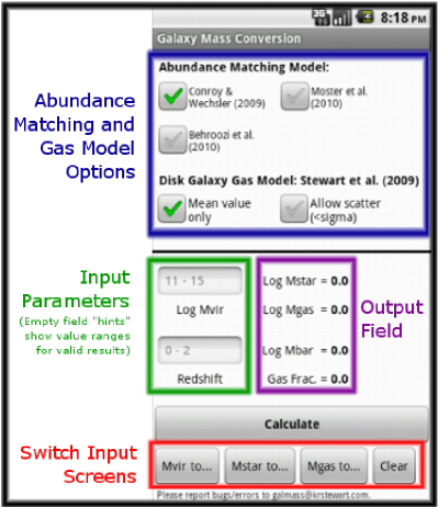
Figure 1.— Screenshot of the GalMass application. The upper (blue) region shows the abundance matching and galaxy gas model options (see §2 and §3). The left (green) and right (purple) regions show the input and output fields, respectively. When the input boxes are empty, they display “hint” values that span typical mass and redshift ranges where the models are applicable. The “Calculate” button reads from the input boxes, applies the proper fitting functions, and updates the output field. The bottom (red) region allows the user to switch screens, changing the input mass parameter from between $M_{\rm vir}$, $M_{\rm star}$, and $M_{\rm gas}$. The bottom right “Clear” button clears all screens of their input and output values.

4. Implementation

Throughout the application, masses are always given in units of solar mass, with log values displayed for compactness. Halo virial mass, galaxy stellar mass, galaxy gas mass, and galaxy baryonic mass (gas and stars) are denoted “Mvir,” “Mstar,” “Mgas,” and “Mbar” respectively. The application also computes the galaxy gas fraction (“Gas Frac.”) defined as $M_{\rm gas}/(M_{\rm gas}+M_{\rm star})$.

The basic layout of GalMass consists of three interchangeable screens, depending on the input parameter desired by the user. The buttons that switch between screens are found at the bottom of each screen. For example, the “Mvir to…” button corresponds to the screen where the halo virial mass is expected as an input, and the galaxy’s stellar and gas masses are given as outputs (see Figure 1).

For a more detailed discussion of what mass regimes and redshifts abundance matching results can be trusted, I refer the reader to the original papers from whence I have derived fitting functions: CW09, M10 and B10. Still, to aid the user in knowing when the calculations are based on extrapolations beyond well-tested regimes, GalMass displays a warning message (but output fields are still populated) if any calculations result in one the following: $M_{\rm vir}>10^{15}M_{\odot}$; $M_{\rm vir}<10^{10}M_{\odot}$; or $M_{\rm star}<10^{8}M_{\odot}$. A more severe warning message is displayed (and output fields are cleared to null values) if any input or output values contain the following: $M_{\rm vir}>10^{16}M_{\odot}$; $M_{\rm star}>10^{13}M_{\odot}$; $z>2$; or any mass $<1M_{\odot}$.

Lastly, I re-emphasize that both the abundance matching data and the galaxy gas models, as implemented here in GalMass, are designed for isolated galaxies. The gas model will almost certainly over-estimate the gas content of satellite galaxies, and abundance matching models typically match stellar masses to dark matter virial masses upon first infall (when the galaxy was last isolated).

References

- Behroozi et al. (2010) Behroozi, P. S., Conroy, C., & Wechsler, R. H. 2010, ApJ, 717, 379
- Berrier et al. (2006) Berrier, J. C., Bullock, J. S., Barton, E. J., Guenther, H. D., Zentner, A. R., & Wechsler, R. H. 2006, ApJ, 652, 56
- Boylan-Kolchin et al. (2011) Boylan-Kolchin, M., Bullock, J. S., & Kaplinghat, M. 2011, MNRAS, 415, L40
- Bullock et al. (2010) Bullock, J. S., Stewart, K. R., Kaplinghat, M., Tollerud, E. J., & Wolf, J. 2010, ApJ, 717, 1043
- Conroy & Wechsler (2009) Conroy, C. & Wechsler, R. H. 2009, ApJ, 696, 620
- Conroy et al. (2006) Conroy, C., Wechsler, R. H., & Kravtsov, A. V. 2006, ApJ, 647, 201
- Erb et al. (2006) Erb, D. K., Steidel, C. C., Shapley, A. E., Pettini, M., Reddy, N. A., & Adelberger, K. L. 2006, ApJ, 646, 107
- Hammer et al. (2009) Hammer, F., Flores, H., Puech, M., Athanassoula, E., Rodrigues, M., Yang, Y., & Delgado-Serrano, R. 2009, submitted to A&A, ArXiv:0903.3962 [astro-ph],
- Kannappan (2004) Kannappan, S. J. 2004, ApJ, 611, L89
- McGaugh (2005) McGaugh, S. S. 2005, ApJ, 632, 859
- Moster et al. (2010) Moster, B. P., Somerville, R. S., Maulbetsch, C., van den Bosch, F. C., Macciò, A. V., Naab, T., & Oser, L. 2010, ApJ, 710, 903
- Shankar et al. (2006) Shankar, F., Lapi, A., Salucci, P., De Zotti, G., & Danese, L. 2006, ApJ, 643, 14
- Stewart (2009) Stewart, K. R. 2009, in Astronomical Society of the Pacific Conference Series, Vol. 419, Galaxy Evolution: Emerging Insights and Future Challenges, ed. S. Jogee, I. Marinova, L. Hao, & G. A. Blanc, 243–+
- Stewart et al. (2009a) Stewart, K. R., Bullock, J. S., Barton, E. J., & Wechsler, R. H. 2009a, ApJ, 702, 1005
- Stewart et al. (2009b) Stewart, K. R., Bullock, J. S., Wechsler, R. H., & Maller, A. H. 2009b, ApJ, 702, 307
- Stewart et al. (2008) Stewart, K. R., Bullock, J. S., Wechsler, R. H., Maller, A. H., & Zentner, A. R. 2008, ApJ, 683, 597
- Tollerud et al. (2011) Tollerud, E. J., Bullock, J. S., Graves, G. J., & Wolf, J. 2011, ApJ, 726, 108
- Wei et al. (2010) Wei, L. H., Kannappan, S. J., Vogel, S. N., & Baker, A. J. 2010, ApJ, 708, 841
- Wright et al. (2009) Wright, S. A., Larkin, J. E., Law, D. R., Steidel, C. C., Shapley, A. E., & Erb, D. K. 2009, ApJ, 699, 421