Combined strong and weak lensing analysis of 28 clusters from the Sloan Giant Arcs Survey

Abstract

We study the mass distribution of a sample of 28 galaxy clusters using strong and weak lensing observations. The clusters are selected via their strong lensing properties as part of the Sloan Giant Arcs Survey (SGAS) from the Sloan Digital Sky Survey (SDSS). Mass modelling of the strong lensing information from the giant arcs is combined with weak lensing measurements from deep Subaru/Suprime-cam images to primarily obtain robust constraints on the concentration parameter and the shape of the mass distribution. We find that the concentration $c_{\rm vir}$ is a steep function of the mass, $c_{\rm vir}\propto M_{\rm vir}^{-0.59\pm 0.12}$, with the value roughly consistent with the lensing-bias-corrected theoretical expectation for high mass ($\sim 10^{15}h^{-1}M_{\odot}$) clusters. However, the observationally inferred concentration parameters appear to be much higher at lower masses ($\sim 10^{14}h^{-1}M_{\odot}$), possibly a consequence of the modification to the inner density profiles provided by baryon cooling. The steep mass-concentration relation is also supported from direct stacking analysis of the tangential shear profiles. In addition, we explore the two-dimensional shape of the projected mass distribution by stacking weak lensing shear maps of individual clusters with prior information on the position angle from strong lens modelling, and find significant evidence for a large mean ellipticity with the best-fit value of $\langle e\rangle=0.47\pm 0.06$ for the mass distribution of the stacked sample. We find that the luminous cluster member galaxy distribution traces the overall mass distribution very well, although the distribution of fainter cluster galaxies appears to be more extended than the total mass.

1 Introduction

Gravitational lensing plays a dominant role in determining the mass distribution of distant galaxies and clusters of galaxies, because it allows direct measurements of the distribution of dark matter which accounts for $\sim 90\%$ of the total matter content of the Universe. Precise measurements of dark matter distributions are important not only for understanding the formation of galaxies in the context of the hierarchical structure formation scenario, but also for testing the properties of the putative dark matter particle, in particular its cold and collisionless nature. Observations of clusters are suitable and very apt for the latter purpose, as the long cooling timescale for hot gas in clusters indicates that the cluster gravitational potential is mainly determined by the dynamics of the dominant dark matter component which are well predicted by $N$-body simulations. However, it is also expected that the baryonic component in clusters, which dominates the mass in the innermost regions, should play an important role at some point.

There are two regimes of gravitational lensing that can be employed to measure and map the mass distribution in clusters. One is strong lensing, i.e., the regime that produces drastic lensing events with highly elongated arcs or multiple images of background objects (e.g., Kochanek, 2006; Kneib & Natarajan, 2011, for reviews). The other lensing regime is weak lensing wherein statistical measurements of small distortions in the shapes of background galaxies are produced by a massive, foreground cluster (e.g., Bartelmann & Schneider, 2001, for a review). Since strong and weak lensing probe mass distributions at different radii, the combination of these two is powerful and essential for the full understanding and detailed mapping of the gravitational potential of clusters.

Lensing studies of clusters have indeed confirmed several important predictions of the standard $\Lambda$-dominated Cold Dark Matter ($\Lambda$CDM) model. For instance, from numerical simulations, the radial run of the density of the mass distribution is predicted to have a universal form, that of the Navarro-Frenk-White profile (e.g., Navarro et al., 1996, 1997). Detailed lensing measurements of massive clusters have confirmed this prediction by and large, although there does appear to be some cluster-to-cluster variations (e.g., Okabe et al., 2010; Umetsu et al., 2011b). Another important prediction is that massive clusters are on average highly non-spherical with a typical major to minor axis ratio of $\sim$2:1 (Jing & Suto, 2002). Weak lensing measurements of dark matter distributions in a sample of massive clusters have directly confirmed this prediction as well (Oguri et al., 2010). Furthermore, lensing analysis of several merging clusters of galaxies strongly supports the collisionless nature of dark matter (Clowe et al., 2006; Jee et al., 2007; Bradač et al., 2008; Merten et al., 2011), although a possible case against the collisionless nature has also been discovered (Mahdavi et al., 2007).

However, measurements of the concentration parameter, which appears in the Navarro-Frenk-White profile, from gravitational lensing observations for clusters have been controversial. The concentration parameter is defined as the ratio of the virial radius to the scale radius, and is a dimensionless parameter that quantifies the degree of the mass accumulation in the innermost regions. The standard $\Lambda$CDM model makes a prediction about this parameter too, namely that more massive haloes or haloes at higher redshifts have smaller values of the concentration parameter on average (e.g., Bullock et al., 2001). However, measurements of the dark matter distribution in the massive lensing cluster A1689 for instance, using both strong and weak lensing, have indicated that the mass distribution is surprisingly highly concentrated with an estimated concentration parameter of $c_{\rm vir}\sim 12$, which is significantly higher than the expected standard $\Lambda$CDM prediction of $c_{\rm vir}\sim 4$ (Broadhurst et al., 2005; Umetsu & Broadhurst, 2008).

The interpretation of this result of lensing clusters being over-concentrated requires careful consideration due to the role played by projection and selection effects. This is because lensing observables can only measure the projected mass distribution, and hence the recovery of the three-dimensional mass distribution requires additional assumptions about the elongation along the line-of-sight direction. For instance, because of the large triaxiality of dark matter haloes, the mass and concentration parameter inferred from gravitational lensing depend strongly on the orientation with respect to the line-of-sight direction. This naturally implies that both the mass and concentration are significantly overestimated when observed along the major axis (Clowe, De Lucia, & King, 2004; Oguri et al., 2005; Gavazzi, 2005; Corless & King, 2007). The large orientation dependence in turn suggests that strong lensing selected clusters represent a highly biased population with their major axes preferentially aligned with the line-of-sight direction (Hennawi et al., 2007; Oguri & Blandford, 2009; Meneghetti et al., 2010). Thus, the dark matter distribution of A1689 alone does not pose a severe challenge to the $\Lambda$CDM model (Oguri et al., 2005; Oguri & Blandford, 2009; Corless et al., 2009; Sereno, Jetzer, & Lubini, 2010; Coe et al., 2010; Morandi, Pedersen, & Limousin, 2011; Sereno & Umetsu, 2011; Morandi et al., 2011), although such high values of the concentration parameter appear to be common in the combined strong and weak lensing analysis of massive clusters (Comerford & Natarajan, 2007; Broadhurst et al., 2008; Oguri et al., 2009; Umetsu et al., 2011b; Zitrin et al., 2011b). High concentrations can be tested with the distribution of the Einstein radii, but the results have still not converged (Broadhurst & Barkana, 2008; Oguri & Blandford, 2009; Richard et al., 2010; Gralla et al., 2011; Zitrin et al., 2011a, c). Also puzzling is the fact that such high concentrations have not been claimed in weak lensing analysis (Okabe et al., 2010) or X-ray analysis (Buote et al., 2007; Ettori et al., 2010) for samples of massive clusters.

While the combined strong and weak lensing analysis allows accurate and robust measurements of the concentration parameter, the current main limitation is the small number of clusters available for such a detailed combined analysis. The Sloan Giant Arcs Survey (SGAS; Hennawi et al., 2008; Bayliss et al., 2011a), which is a survey of strongly lensed giant arcs from the Sloan Digital Sky Survey (SDSS; York et al., 2000), has already discovered more than 30 bright giant arcs and therefore offers an ideal technique to expand the sample of clusters appropriate for detailed lensing analysis.

In this paper, we present a systematic study of strong and weak lensing analysis for a sample of 28 clusters from the SGAS, based on our extensive follow-up imaging observations with Subaru/Suprime-cam (Miyazaki et al., 2002). We study the radial dark matter distributions of the clusters in detail to measure the concentration parameters for these clusters. For this purpose we conduct a stacked lensing analysis as well as individual modelling of clusters. With the stacked lensing technique we also study the two-dimensional mass distribution, and constrain the ellipticity of the projected mass distribution.

The structure of this paper is as follows. We describe our cluster sample and follow-up imaging observations with Subaru/Suprime-cam in Section 2, and present the strong and weak lensing analysis in Section 3. The results are combined to discuss the mass-concentration relation in Section 4. We also conduct a stacked lensing analysis, which is detailed in Section 5. We then study the cluster member galaxy distribution in Section 6, and summarize the main conclusions in Section 7. In Appendix A we conduct semi-analytic calculations to evaluate the effect of the lensing bias on various observables. Appendix B summarizes the strong and weak lensing analysis results of individual clusters. Throughout the paper we assume the standard $\Lambda$-dominated flat cosmological model with the matter density $\Omega_{M}=1-\Omega_{\Lambda}=0.275$, the dimensionless Hubble constant $h=0.702$, the baryon density $\Omega_{b}h^{2}=0.02255$, the spectral index $n_{s}=0.968$, and a normalization for the matter power spectrum $\sigma_{8}=0.816$ (Komatsu et al., 2011) where needed.

2 Cluster sample and follow-up observations

2.1 Cluster sample

We draw our sample of clusters for detailed lensing analysis from SGAS, which involved an initial extensive visual search of giant arcs in red-sequence selected clusters in the SDSS. The sample is constructed utilizing two selection methods. One is the SDSS “Visual” survey which selects giant arc candidates from the visual inspection of the SDSS imaging data (M. D. Gladders et al., in preparation). The other survey is the SDSS “Blind” survey which searches for giant arcs from $g$-band follow-up imaging of the most massive $\sim 200$ clusters selected from the SDSS imaging data (Hennawi et al., 2008). Some of the clusters have also been reported in Wen et al. (2011). We are conducting massive spectroscopic follow-up observations of these new giant arcs with the Gemini Multi-Object Spectrograph (GMOS; Hook et al., 2004) to measure redshifts for the newly discovered arcs as well as redshifts for the lensing clusters. See Bayliss et al. (2011b) for details of our spectroscopic follow-up and successful redshift measurements for more than 20 giant arcs. We note that this paper includes a few new GMOS spectroscopy results obtained after the publication of Bayliss et al. (2011b). We also include two cluster-scale quasar lenses discovered from the SDSS Quasar Lens Search (SQLS; Oguri et al., 2006, 2008a; Inada et al., 2008, 2010), as they satisfy similar selection criteria to the SGAS lens sample, and have also been observed at the Subaru telescope.

Table 1: Cluster sample and summary of Subaru/Suprime-cam imaging observations. The redshifts of the clusters are taken from Bayliss et al. (2011b).

Name	R.A.	Decl.	$z$	Exp ($g$)	Seeing ($g$)	Exp ($r$)	Seeing ($r$)	Exp ($i$)	Seeing ($i$)
	(J2000)	(J2000)		(sec)	(arcsec)	(sec)	(arcsec)	(sec)	(arcsec)
SDSSJ0851+3331	08 51 38.86	+33 31 06.1	0.370	1200	0.79	1800	1.05	1680	0.71
SDSSJ0915+3826	09 15 39.00	+38 26 58.5	0.397	1200	0.89	2100	0.87	1680	0.67
SDSSJ0957+0509	09 57 39.19	+05 09 31.9	0.448	1200	1.01	2100	0.61	1680	0.81
SDSSJ1004+4112	10 04 34.18	+41 12 43.5	0.68	810	0.71	1210	0.67	1340	0.61
SDSSJ1029+2623	10 29 12.48	+26 23 32.0	0.584	1200	0.79	2700	0.65	1920	1.05
SDSSJ1038+4849	10 38 42.90	+48 49 18.7	0.430	900	0.75	2100	0.79	1680	0.83
SDSSJ1050+0017	10 50 39.90	+00 17 07.1	0.60a	1200	0.59	2100	0.67	1680	0.65
RCS2J1055+5547	10 55 04.59	+55 48 23.3	0.466	1200	0.95	2100	0.89	1440	0.83
SDSSJ1110+6459	11 10 17.70	+64 59 47.8	0.659b	1200	1.23	2100	0.89	1680	1.05
SDSSJ1115+5319	11 15 14.85	+53 19 54.6	0.466	1200	1.39	1500	1.13	1200	1.13
SDSSJ1138+2754	11 38 08.95	+27 54 30.7	0.451	900	0.81	2100	0.85	1440	0.85
SDSSJ1152+3313	11 52 00.15	+33 13 42.1	0.362	1200	1.17	1800	0.55	1680	1.21
SDSSJ1152+0930	11 52 47.38	+09 30 14.7	0.517	1200	1.13	2100	1.01	1200	0.93
SDSSJ1209+2640	12 09 23.68	+26 40 46.7	0.561	1200	1.25	2100	0.79	960	1.13
SDSSJ1226+2149c	12 26 51.11	+21 49 52.3	0.435	1200	1.05	$R_{\rm c}$=2170	0.81	1680	0.91
A1703	13 15 05.24	+51 49 02.6	0.277	1200	0.97	2100	0.91	1200	0.87
SDSSJ1315+5439	13 15 09.30	+54 37 51.8	0.588d	1200	0.69	1500	0.91	1680	0.71
GHO132029+3155	13 22 48.77	+31 39 17.8	0.308	1200	0.77	2100	0.81	1680	0.87
SDSSJ1329+2243	13 29 34.49	+22 43 16.2	0.443d	1200	0.69	2100	0.85	1680	0.69
SDSSJ1343+4155	13 43 32.85	+41 55 03.4	0.418	1200	0.83	1500	0.83	1440	1.33
SDSSJ1420+3955	14 20 40.33	+39 55 09.8	0.607	1200	1.29	1800	0.79	1440	0.73
SDSSJ1446+3032	14 46 34.02	+30 32 58.2	0.464	1200	0.85	2100	0.83	1200	0.93
SDSSJ1456+5702	14 56 00.78	+57 02 20.3	0.484	1200	0.71	2100	0.81	1440	1.11
SDSSJ1531+3414	15 31 10.60	+34 14 25.0	0.335	1200	0.91	1500	0.99	1200	1.01
SDSSJ1621+0607	16 21 32.36	+06 07 19.0	0.342	1500	0.77	2100	0.85	1440	1.31
SDSSJ1632+3500	16 32 10.26	+35 00 29.7	0.49a	900	0.85	2100	0.77	1440	0.77
SDSSJ2111$-$0114	21 11 19.34	$-$01 14 23.5	0.638	1440	0.83	2400	0.61	1680	0.53

2.2 Observations with Subaru/Suprime-cam

We observed the SGAS giant arc clusters with Suprime-cam (Miyazaki et al., 2002) at the Subaru 8.2-meter telescope, primarily for the wide-field weak lensing analysis, between 2007 June and 2011 April. Combined with a few images retrieved from the archive system named SMOKA (Baba et al., 2002), our sample comprises 28 clusters with Subaru/Suprime-cam multicolour follow-up imaging. The Suprime-cam has a large field-of-view of $\sim 34^{\prime}\times 27^{\prime}$ with a pixel scale of $0\aas@@fstack{\prime\prime}202$, and is therefore ideal for weak lensing studies of massive clusters at intermediate redshifts whose typical virial radius is $\la 10^{\prime}$. Our strategy is to obtain deep images in $g$-, $r$-, and $i$-bands, with the longest exposure in $r$-band. The deep $r$-band imaging is performed to conduct weak lensing analysis using $r$-band images, but the additional colour information from $g$- and $i$-bands are crucial for reliable selection of background galaxies for the weak lensing analysis (more details presented in Section 3.2) as well as secure identifications of multiply imaged arcs in the cluster cores. We note that the weak lensing analysis results of the first 4 SGAS clusters have been published in Oguri et al. (2009).

The data are reduced using SDFRED and SDFRED2 (Yagi et al., 2002; Ouchi et al., 2004). The reduction procedure includes bias subtraction, flat-fielding, distortion correction, sky subtraction, and co-adding to generate the final mosaic images. When co-adding, we remove some of the frames which have significantly worse seeing sizes than other frames. We derive the magnitude zero-points by comparing objects in the reduced images with the photometric catalogue of the SDSS data. The astrometric calibration is performed with SCAMP (Bertin, 2006), again using objects in the SDSS data as astrometric reference sources. The photometric galaxy catalogue of each cluster is constructed using SExtractor (Bertin & Arnouts, 1996), with the Galactic extinction correction (Schlegel, Finkbeiner, & Davis, 1998). Our 28 cluster sample and basic parameters of follow-up images are summarized in Table 1.

3 Strong and weak lensing analysis

3.1 Strong lensing analysis

We mostly follow Oguri et al. (2009) for the strong lens modelling methodology. Basically we assume the elliptical extension of the NFW profile (Navarro et al., 1996, 1997) to model the mass distribution of a dark halo, and add contributions from member galaxies assuming the pseudo-Jaffe model.The velocity dispersion $\sigma$ and cutoff scale $r_{\rm cut}$ of the pseudo-Jaffe model are assumed to scale with the luminosity as $L\propto\sigma^{1/4}$ and $r_{\rm cut}\propto L^{1/2}$. The normalization and cut-off radius may be fixed to a typical value if there are not enough observational constraints. We may also fix the centre of the main halo to the position of the brightest cluster galaxy, depending on the number of available constraints and the configuration of multiple images.

We identify multiple images based on spectroscopic follow-up results of Bayliss et al. (2011b) as well as colours of lensed arcs measured from the Subaru/Suprime-cam images. While redshifts of arcs are available for many of our sample clusters, for clusters without any arc spectroscopy information we assume that the redshift of the main arc is $z_{\rm arc}=2$ with the conservative 1$\sigma$ error of $\sigma(z_{\rm arc})=1$, because our extensive spectroscopic observations (Bayliss et al., 2011a) as well as photometric analysis (Bayliss, 2011) have convincingly shown that most of the arcs in our sample fall in this redshift range. The positional uncertainties of all the arcs are assumed to be $1^{\prime\prime}$ in the image plane, which is much larger than measurement uncertainties but is typical of the uncertainties associated with parametric strong lens modelling of clusters.

We perform strong lens modelling using the software glafic (Oguri, 2010), using the $\chi^{2}$ minimization in the source plane (see Oguri et al., 2009; Oguri, 2010). From the derived best-fit mass model we compute the Einstein radius $\theta_{\rm E}$ of the system by solving the following equation:

$$\bar{\kappa}(<\theta_{\rm E})=\frac{1}{\pi\theta_{\rm E}^{2}}\int_{|\mbox{\boldmath$\theta$}|<\theta_{\rm E}}\kappa(\mbox{\boldmath$\theta$})d\mbox{\boldmath$\theta$}=1,$$ (1)

and use only this Einstein radius determination as the constraint from our strong lensing analysis. We use the Einstein radius as it is a robust quantity that is well constrained from the strong lensing modelling and is fairly insensitive to our model assumptions (e.g., Jullo et al., 2007). We estimate the error on the Einstein radius by changing one (usually mass) of the parameters from the best-fit values, optimizing other parameters, and monitoring the $\chi^{2}$ differences. However, to be conservative in our estimates, we always assign a minimum error of $10\%$ to the Einstein radius, even if the procedure above returns smaller errors, given the unaccounted complexity of cluster mass distributions and projections along line-of-sight (e.g., D’Aloisio & Natarajan, 2011). For clusters without arc spectroscopy, we conservatively estimate the $1\sigma$ error on the Einstein radius by changing the arc redshift by $\pm 1$. The Einstein radii are computed for both the arc redshift $z_{\rm arc}$ and the fixed source redshift of $z_{s}=2$. We use the former value for the combined strong and weak lensing analysis, whereas the latter value is used for the statistical, stacked lensing analysis.

We note that the definition of the Einstein radius adopted here differs from that in Oguri et al. (2009). In this new definition the contribution of stellar masses is explicitly included, while in Oguri et al. (2009) the Einstein radius was computed from the dark halo component alone. The use of this modified definition is because the separation of dark and luminous components is not obvious, and has to rely on several assumptions, unless we have additional data such as the velocity dispersion measurement of the central galaxy (e.g., Sand et al., 2008; Newman et al., 2009). Thus the effect of baryonic components has been taken into account in interpreting our results.

Table 2: Summary of strong lensing analysis. We tabulate the Einstein radii both for arc redshifts and for $z_{s}=2$, the total number of multiple images used for strong lens modelling ($N_{\rm img}$; the number of multiple image sets is shown in parentheses), the best-fit ellipticity ($e$) and position angle ($\theta_{e}$) of the main dark halo component, and references for arc redshifts.

Name	$z_{\rm arc}$a	$N_{\rm img}$	$\theta_{\rm E}$ ($z_{s}=z_{\rm arc}$)	$\theta_{\rm E}$ ($z_{s}=2$)	$e$	$\theta_{e}$b	Ref.c
			(arcsec)	(arcsec)		(deg)
SDSSJ0851+3331	1.693	4(1)	$21.6^{+2.2}_{-2.2}$	$23.0^{+2.3}_{-2.3}$	0.23	$39.1$	1
SDSSJ0915+3826	1.501	3(1)	$9.8^{+1.3}_{-1.0}$	$11.4^{+1.3}_{-1.1}$	0.28	$-74.9$	1,2
SDSSJ0957+0509	1.820	3(1)	$5.2^{+0.5}_{-0.5}$	$5.4^{+0.5}_{-0.5}$	0.82	$64.2$	1,3
SDSSJ1004+4112	1.734	31(8)	$7.3^{+0.7}_{-0.7}$	$8.9^{+0.9}_{-0.9}$	0.14	$-28.0$	4,5
SDSSJ1029+2623	2.197	3(1)	$10.7^{+4.8}_{-6.1}$	$9.9^{+4.8}_{-5.9}$	0.58	$-81.5$	6,7
SDSSJ1038+4849	2.198	9(3)	$12.6^{+1.3}_{-1.6}$	$11.2^{+1.5}_{-1.4}$	0.15	$-52.8$	1,8,9
SDSSJ1050+0017	$2\pm 1$	3(1)	$16.1^{+17.9}_{-2.5}$	$16.1^{+17.9}_{-2.5}$	0.28	$-6.9$
RCS2J1055+5548	1.250	3(1)	$10.0^{+1.0}_{-1.0}$	$12.7^{+1.3}_{-1.3}$	0.82	$3.2$	1
SDSSJ1110+6459	$2\pm 1$	3(1)	$8.4^{+12.7}_{-1.5}$	$8.4^{+12.7}_{-1.5}$	0.60	$76.9$
SDSSJ1115+5319	$2\pm 1$	5(1)	$21.9^{+18.2}_{-3.4}$	$21.9^{+18.2}_{-3.4}$	0.63	$-47.4$
SDSSJ1138+2754	1.334	5(2)	$9.8^{+1.0}_{-1.5}$	$12.9^{+1.3}_{-3.6}$	0.50	$-18.7$	1
SDSSJ1152+3313	2.491	7(2)	$8.7^{+0.9}_{-0.9}$	$8.2^{+0.8}_{-0.8}$	0.34	$64.5$	1
SDSSJ1152+0930	$2\pm 1$	3(1)	$4.5^{+8.2}_{-0.7}$	$4.5^{+8.2}_{-0.7}$	0.80	$-38.5$
SDSSJ1209+2640	1.021	6(2)	$8.8^{+0.9}_{-0.9}$	$21.3^{+2.1}_{-2.1}$	0.14	$66.1$	1,10
SDSSJ1226+2149	1.605	3(1)	$14.0^{+3.4}_{-2.6}$	$15.7^{+3.8}_{-2.8}$	0.47	$-57.5$	1
SDSSJ1226+2152	2.923	3(1)	$10.0^{+2.8}_{-6.4}$	$8.6^{+2.4}_{-5.5}$	0.18	$12.3$	1,11
A1703	2.627	21(6)	$27.4^{+2.7}_{-2.7}$	$25.3^{+2.5}_{-2.5}$	0.33	$-26.2$	1,12,13
SDSSJ1315+5439	$2\pm 1$	3(1)	$16.9^{+20.6}_{-2.9}$	$16.9^{+20.6}_{-2.9}$	0.18	$-36.8$
GHO132029+3155	$2\pm 1$	4(1)	$21.5^{+7.0}_{-2.2}$	$21.5^{+7.0}_{-2.2}$	0.10	$76.5$
SDSSJ1329+2243	2.040	3(1)	$10.9^{+1.6}_{-1.6}$	$10.8^{+1.6}_{-1.6}$	0.22	$-4.9$	14
SDSSJ1343+4155	2.091	3(1)	$5.4^{+2.5}_{-1.6}$	$5.3^{+2.5}_{-1.6}$	0.73	$64.9$	1,2,15
SDSSJ1420+3955	2.161	6(2)	$9.9^{+2.8}_{-1.0}$	$9.4^{+2.7}_{-0.9}$	0.77	$73.6$	1
SDSSJ1446+3032	$2\pm 1$	4(1)	$16.8^{+13.1}_{-2.3}$	$16.8^{+13.1}_{-2.3}$	0.22	$-41.6$
SDSSJ1456+5702	0.833	6(2)	$13.2^{+1.3}_{-1.3}$	$30.1^{+9.2}_{-5.0}$	0.21	$-13.6$	1
SDSSJ1531+3414	1.096	6(2)	$11.7^{+1.2}_{-1.2}$	$16.6^{+1.7}_{-1.7}$	0.09	$-37.5$	1
SDSSJ1621+0607	4.131	3(1)	$12.5^{+1.5}_{-2.5}$	$10.3^{+1.3}_{-2.2}$	0.33	$-40.0$	1
SDSSJ1632+3500	$2\pm 1$	4(1)	$14.3^{+12.6}_{-2.1}$	$14.3^{+12.6}_{-2.1}$	0.30	$-61.9$
SDSSJ2111$-$0114	2.858	9(3)	$17.7^{+10.6}_{-5.8}$	$14.5^{+9.2}_{-4.8}$	0.24	$10.0$	1

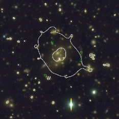
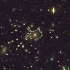
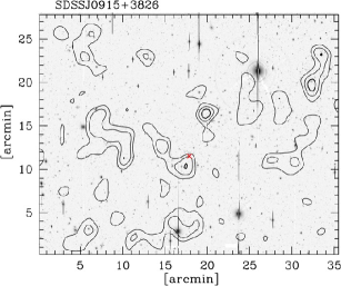
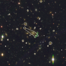
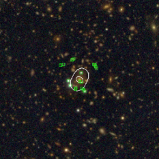
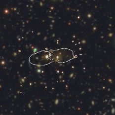
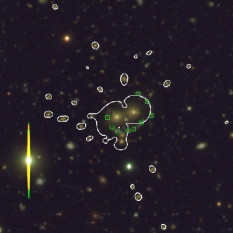
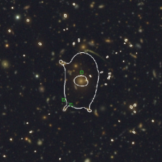
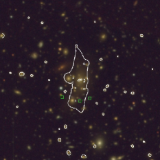
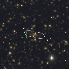
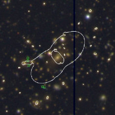
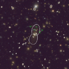
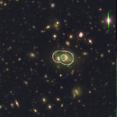
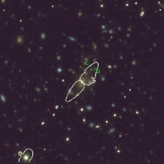
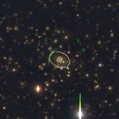
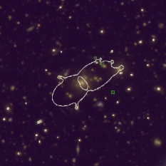
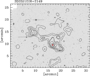
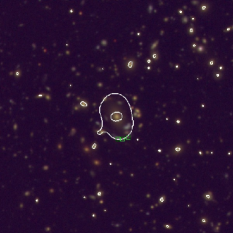
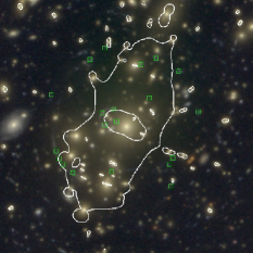
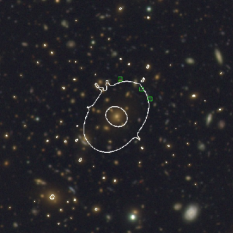
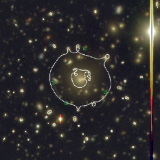
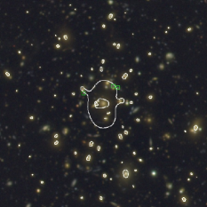
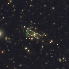
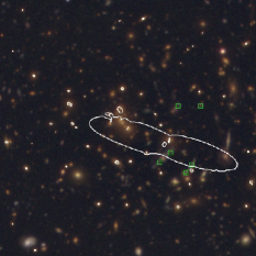
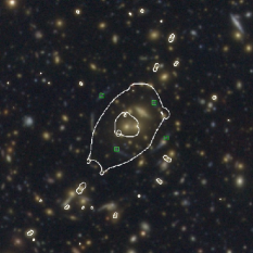
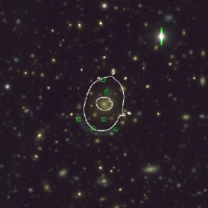
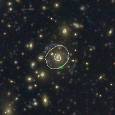
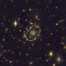
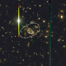
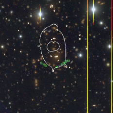
Table 2 lists the Einstein radii derived from strong lensing modelling. SDSSJ1226+2149 and SDSSJ1226+2152 are two nearby strong lensing cores in a highly complex massive structure, both of which are covered by our Subaru/Suprime-cam imaging (Bayliss et al., 2011b). We perform strong lensing analysis for both cores. We also show the best-fit ellipticity $e$ and the position angle $\theta_{e}$ of the best-fit main NFW component, as they are used later for two-dimensional stacking analysis (Section 5.2). The best-fit critical curves for individual clusters are presented in Appendix B.

Strong lensing analysis for some of these clusters has been published in the literature (e.g., Oguri et al., 2009; Koester et al., 2010; Bayliss et al., 2010; Oguri, 2010; Gralla et al., 2011). Our estimates of the Einstein radii presented here generally agree with these previous results. For A1703, our best-fit Einstein radius is in excellent agreement with that of the independent strong lens modelling by Richard et al. (2009). An exception is SDSSJ1343+4155 whose Einstein radius in our strong lens modelling result is much smaller than what presented in Bayliss et al. (2010) and Gralla et al. (2011) because a large offset of the halo centre from the brightest cluster galaxy has been found in the previous analysis, whereas in the present paper the centre of the halo is fixed to the location of the brightest cluster galaxy.

3.2 Weak lensing analysis

For weak lensing measurements, we follow the formalism outlined in Kaiser et al. (KSB; 1995) using the software package IMCAT. We first detect objects in the reduced images using a hierarchical peak finding algorithm. For all the clusters in our sample, we use $r$-band images for weak lensing shear measurements. We then measure the shapes of objects by iteratively refining the centroid of each object. Stars for correcting the distortion of the Point Spread Function (PSF) are selected in a standard way by identifying the appropriate branch in the magnitude-half light radius $r_{h}$ plane, along with the peak significance cut $\nu>15$. Shapes of the stars are measured as a function of the size of the weight function, $r_{g}$, in order to make PSF corrections with matched $r_{g}$ values. We divide each co-added image into $4\times 3$ chunks and fit the PSF in each chunk independently with second order bi-polynomials. The smear polarizability is corrected by computing a scalar polarizability $P_{s}$ from the trace of the matrix, and then fitting $P_{s}$ as a function of magnitude, $r_{g}$, and the galaxy ellipticity. For our weak lensing analysis, we only use galaxies with $\nu>15$ and $r_{h}>\overline{r_{h}^{*}}+2\sigma(r_{h}^{*})$, where $\overline{r_{h}^{*}}$ and $\sigma(r_{h}^{*})$ are median and root-mean-square dispersion of half-light radii for the stars selected above. Given the general tendency of the KSB algorithm to underestimate the weak lensing shear (Erben et al., 2001; Heymans et al., 2006; Massey et al., 2007), we include a calibration factor of $1/0.9$, i.e., this factor is multiplied to all the estimated shear values. For each object we assign the statistical weight $w_{g}$ defined by (e.g., Hamana et al., 2003; Miyazaki et al., 2007; Hamana et al., 2009; Okabe et al., 2010; Okabe, Okura, & Futamase, 2010; Umetsu et al., 2010, 2011b).

$$w_{g}=\frac{1}{\sigma_{g}^{2}+\alpha^{2}},$$ (2)

with $\alpha=0.4$ and $\sigma_{g}$ is the variance of the shear computed from 20 neighbors in the magnitude-$r_{g}$ plane. When computing shear by averaging shear measurements of galaxies in a bin, we also apply a $3\sigma$ clipping which appears to reduce the shear measurement bias.

To check the accuracy of the weak lensing shear measurement, we perform a series of image simulations. Specifically, we generate a galaxy catalogue using the software Stuff (Bertin, 2009). Each galaxy is described by the sum of bulge and disk components, which we model with Sersic profiles with the index $n=4$ and $n=1$, respectively. We also add stars in the catalogue. We convolve the image with a PSF which we assume follows the Moffat profile $\Sigma(r)\propto[1+(r/a)^{2}]^{-\beta}$ with an elliptical extension. Based on the catalogue, we generate a number of realistic Subaru/Suprime-cam like images with different seeing sizes ($0\aas@@fstack{\prime\prime}5$–$1\aas@@fstack{\prime\prime}1$) and $\beta$ ($3<\beta<12$) using the software glafic (Oguri, 2010). We find that the resulting shear multiplicative error (the parameter $m$ in Heymans et al., 2006; Massey et al., 2007) depends on both seeing size and $\beta$ such that $m$ is smaller for larger seeing sizes or smaller $\beta$, but our algorithm generally yields $|m|\la 0.05$ for a wide range of PSF parameters examined here.

3.3 Galaxy selection in colour-colour space

A careful selection of background galaxies is essential for cluster weak lensing studies, because contamination by cluster member galaxies is known to dilute the detected weak lensing signal significantly, particularly near the cluster centres (e.g., Broadhurst et al., 2005; Medezinski et al., 2007). Our $gri$-band imaging is very powerful for reliable background galaxy selection, because we can select galaxies efficiently in colour-colour space (Medezinski et al., 2010).

Figure 1: Upper: The colour cut selecting background galaxies for weak lensing analysis (shading). The colour cut for red member galaxy selection is indicated by dotted lines. The four regions correspond to colour cuts for different cluster redshifts. Solid contours indicate galaxy number density in the COSMOS catalogue ($i<25$). lower: Photometric redshift distributions of galaxies in the COSMOS catalogue, before (dotted) and after (solid) the colour cut.

We determine the colour cut that is appropriate for our cluster sample based on the COSMOS photometric galaxy catalogue (Ilbert et al., 2009). Thanks to the wide wavelength coverage from the ultraviolet to mid-infrared, the photometric redshifts are very accurate down to $i\sim 25$. By inspecting the photometric redshift distributions in each point of the $g-r$ versus $r-i$ colour space, we determine the colour cut for our analysis as

$$g-r>1\;\;\mbox{\&\&}\;\;r-i<0.4(g-r)-0.5,$$ (3)

$$g-r<0.3,$$ (4)

$$r-i>1.3,$$ (5)

$$r-i>g-r,$$ (6)

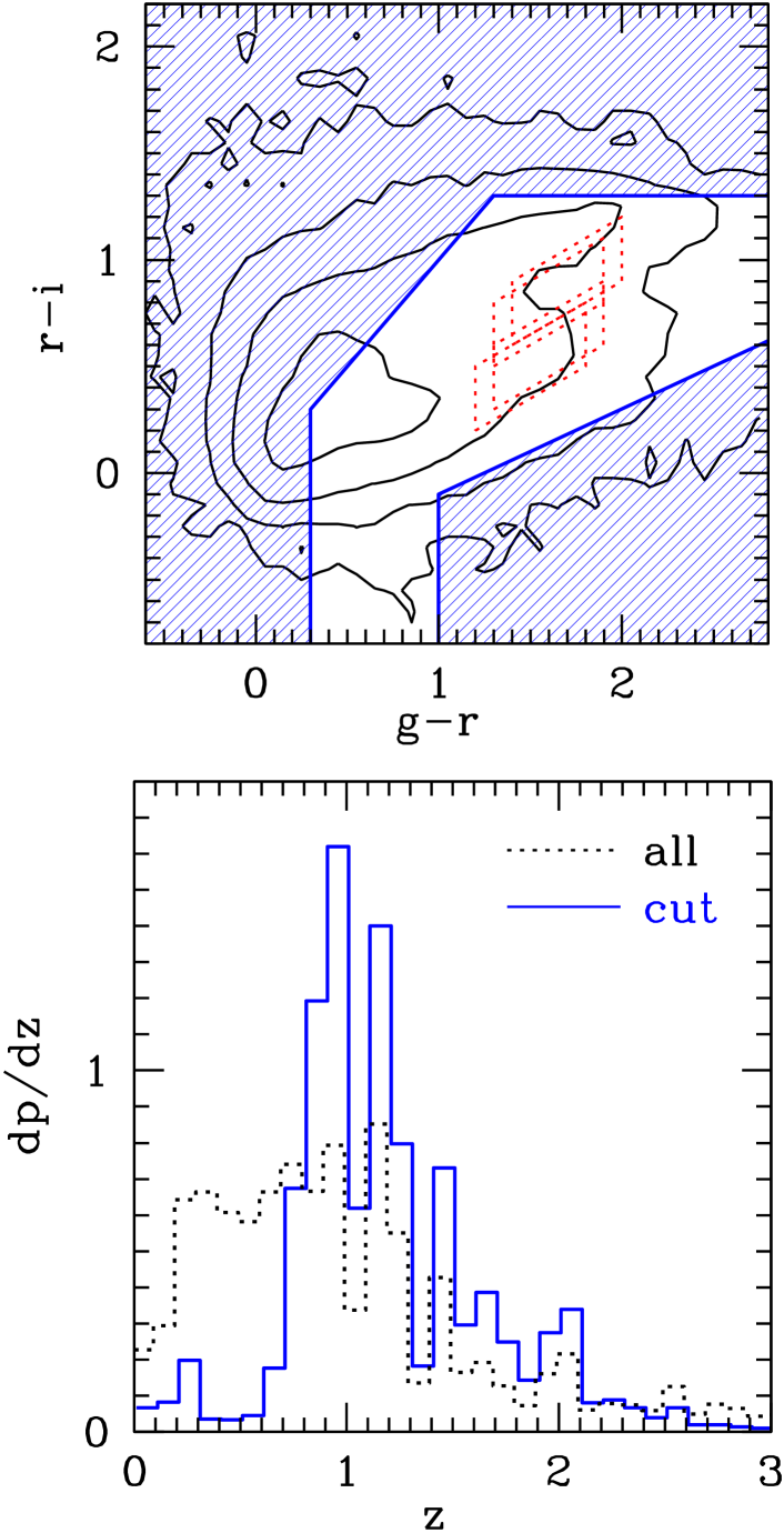
Figure 1 shows the cut and resulting COSMOS photometric redshift distribution. It is seen that our cut efficiently selects galaxies at $z\ga 0.7$, the redshifts higher than any cluster redshifts in our sample. In our weak lensing analysis, we also limit the range of $r$-band magnitude to $21<r<r_{\rm lim}$, where the limiting magnitude $r_{\rm lim}$ is determined from the galaxy number counts of each cluster field image (see below).

In addition to background galaxies, we identify cluster (red) member galaxies by the following criteria:

$$a_{1}-0.3<g-r<a_{1}+0.3,$$ (7)

$$0.5(g-r)+a_{2}-0.15<r-i<0.5(g-r)+a_{2}+0.15,$$ (8)

with ($a_{1}$, $a_{2}$) are ($1.5$, $-0.25$) for $z<0.35$, ($1.6$, $-0.22$) for $0.35<z<0.45$, ($1.6$, $0$) for $0.45<z<0.55$, and ($1.7$, $0.05$) for $0.55<z$. These cuts are also indicated by the upper panel of Figure 1.

Figure 2: The radial number density distributions of galaxies, which are obtained by averaging distributions over all 28 clusters. We show distributions for background galaxies (open circles), cluster member galaxies (filled squares), and “field” galaxies (filled triangles) that are simply defined as being neither member nor background galaxies. Note that the distributions are normalized by the overall number densities.

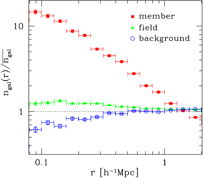
Figure 2 shows the average radial number density distributions of galaxies, background, member, and field (i.e., galaxies which are neither background nor member) galaxies in our 28 cluster sample. As expected, the member galaxy density is steeply rising near the cluster. Field galaxies do not show strong dependence on the distance from the centre, as that should be dominated by local foreground galaxies. A slight increase at small radius suggests that some blue cluster member galaxies are included in the field galaxy sample. On the other hand, background galaxy density decreases near the centre, which is in fact expected because of the lensing magnification and dilution effect of clusters (e.g., Broadhurst et al., 2005; Umetsu et al., 2011a). These distributions basically support the successful colour cut for selecting background galaxies.

Figure 3: The mean galaxy redshift as a function of $i$-band magnitude, which is derived from the COSMOS photometric redshift catalogue (Ilbert et al., 2009). The solid line plots our fit given by equation (12).

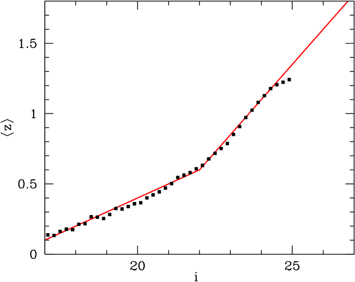
In order to extract physical quantities for clusters from weak lensing signals, we need an estimate of the lensing depth of our source galaxy sample. Again, the COSMOS photometric redshift catalogue is useful for this purpose, but one problem is that many of our source galaxies are fainter than the magnitude limit of the COSMOS photometric redshift catalogue. To overcome this problem, we adopt the following procedure to estimate the lensing depth. First, from the COSMOS photometric redshift catalogue (Ilbert et al., 2009) we derive the response function for our colour cut as $\phi_{\rm cut}(z)=n_{\rm cut}(z)/n_{\rm tot}(z)$, where $n_{\rm tot}(z)$ and $n_{\rm cut}(z)$ are photometric redshift distributions of galaxies before and after the colour cut, respectively. Our weak lensing analysis involves the statistical weight $w_{g}$ (equation 2), and hence we compute the mean weight as a function of $i$-band magnitude as well, $\overline{w_{g}}(i)$, from the background galaxy catalogue. Next we derive the redshift distribution of galaxies as a function of the $i$-band magnitude as follows. First, we adopt the functional form proposed by Schrabback et al. (2010):

$$p(z|i)\propto\left(\frac{z}{z_{0}}\right)^{\alpha}\left(\exp\left[-\left(\frac{z}{z_{0}}\right)^{\beta}\right]+cu^{d}\exp\left[-\left(\frac{z}{z_{0}}\right)^{\gamma}\right]\right),$$ (9)

with $u={\rm max}(0,i-23)$ and ($\alpha$, $\beta$, $c$, $d$, $\gamma$)$=$(0.678, 5.606, 0.581, 1.851, 1.464). We then recompute the mean galaxy redshift as a function of $i$-band magnitude for the range $17<i<25$ using the COSMOS photometric redshift catalogue. The result shown in Figure 3 suggests that it is well approximated by

$$\langle z\rangle=\left\{\begin{array}[]{ll}0.1(i-22)+0.6&\mbox{($17<i<22$)},\\ 0.25(i-22)+0.6&\mbox{($22<i$)},\end{array}\right.$$ (12)

We extrapolate this linear relation to a fainter magnitude of $i>25$, because Schrabback et al. (2010) has explicitly shown that such extrapolation can explain the redshift distribution of galaxies reasonably well down to $i\sim 27$. Using this relation, we derive the relation between $z_{0}$ in equation (9) and $i$-band magnitude, which is approximated by

$$z_{0}=\left\{\begin{array}[]{ll}0.16(i-22)+0.97&\mbox{($17<i<22$)},\\ 0.4(i-22)+0.97&\mbox{($22<i<23.1$)},\\ 1.41&\mbox{($23.1<i<24.3$)},\\ 0.2(i-24.3)+1.41&\mbox{($24.3<i$)}.\end{array}\right.$$ (17)

Using this redshift distribution, we derive the mean depth as

$$\left\langle\frac{D_{ls}}{D_{os}}\right\rangle=\left(\int di\,\overline{D_{i}}\frac{dN}{di}\overline{w_{g}}(i)\right)\left(\int di\,\frac{dN}{di}\overline{w_{g}}(i)\right)^{-1},$$ (18)

$$\overline{D_{i}}=\left(\int dz\frac{D_{ls}}{D_{os}}p(z|i)\phi_{\rm cut}(z)\right)\left(\int dz\,p(z|i)\phi_{\rm cut}(z)\right)^{-1},$$ (19)

where $dN/di$ are the $i$-band number counts of background galaxies used for weak lensing analysis. We define the effective source redshift $z_{s,{\rm eff}}$ such that it reproduces the mean depth:

$$\frac{D_{ls}}{D_{os}}(z_{s,{\rm eff}})=\left\langle\frac{D_{ls}}{D_{os}}\right\rangle.$$ (20)

Throughout this paper, we assume that all the galaxies are located at $z_{s,{\rm eff}}$ for our weak lensing analysis.

The depth estimate above can be affected by the lensing magnification, because the magnification enhances the effective lensing depth. However, the magnification factor tends to decrease rapidly beyond the Einstein radius such that a typical magnification factor of the innermost radial bin for our weak lensing analysis is $\sim 20\%$ or so. This corresponds to the enhancement of the shear amplitude of $\sim 5\%$, which is not significant compared with other uncertainties. Moreover the effect is much smaller at radii where weak lensing signals mostly come from. Thus we conclude that the magnification effect is insignificant for our analysis. Photometric errors that become larger for fainter galaxies can smear the distribution in the color-color space, and hence can affect the lensing depth estimate, but photometric errors are included in the COSMOS photometric redshift catalog as well. Photometric errors for the faintest galaxies in our weak lensing analysis are similar to those for the faintest galaxies in the COSMOS catalog. Another possible systematic effect is the size cut, which may systematically eliminate galaxies at high redshifts and hence bias the lensing depth estimate. While we expect the effect to be small because of the conservative magnitude limit we adopt and the narrow redshift distribution after the color cut, we leave the detailed exploration of this effect for future work.

Table 3: Summary of the weak lensing analysis. We show the median of stellar ellipticities before ($e^{*}_{\rm raw}$) and after ($e^{*}_{\rm cor}$) the PSF correction (numbers in parentheses are standard deviations), the number of stars used for the PSF correction ($N^{*}$), the number density of source background galaxies ($n_{g}$), the $r$-band magnitude limit of source background galaxies ($r_{\rm lim}$), the mean lensing depth ($\langle D_{ls}/D_{os}\rangle$) and the effective source redshift ($z_{s,{\rm eff}}$), the range of the radii for tangential shear fitting ($\theta$ range), and the total signal-to-noise ratio of the tangential shear profile ($S/N$).

Name	$e^{*}_{\rm raw}$	$e^{*}_{\rm cor}$	$N^{*}$	$n_{g}$	$r_{\rm lim}$	$\langle D_{ls}/D_{os}\rangle$	$z_{s,{\rm eff}}$	$\theta$ range	$S/N$
	($10^{-2}$)	($10^{-2}$)		(arcmin-2)	(mag)			(arcmin)
SDSSJ0851+3331	1.51(0.90)	0.01(0.47)	834	10.1	25.8	0.595	1.098	0.63–15.85	6.93
SDSSJ0915+3826	1.40(0.83)	0.02(0.54)	694	11.7	25.6	0.571	1.109	0.40–6.31	4.59
SDSSJ0957+0509	1.28(1.74)	0.01(0.93)	965	11.6	26.0	0.536	1.155	0.40–6.31	3.68
SDSSJ1004+4112	0.26(2.39)	0.02(1.15)	579	8.3	25.4	0.318	1.113	0.40–6.31	2.41
SDSSJ1029+2623	1.27(1.75)	0.01(0.64)	654	17.5	26.2	0.427	1.189	0.40–15.85	7.30
SDSSJ1038+4849	1.58(1.22)	0.03(0.54)	532	12.7	26.0	0.549	1.142	0.40–6.31	3.61
SDSSJ1050+0017	2.00(1.59)	0.02(0.72)	764	16.2	26.0	0.405	1.162	0.50–12.59	7.52
RCS2J1055+5548	1.78(1.33)	0.01(0.52)	569	13.2	25.8	0.513	1.133	0.63–10.00	7.45
SDSSJ1110+6459	3.20(1.50)	0.03(0.75)	924	11.3	25.8	0.407	1.124	0.40–2.51	4.10
SDSSJ1115+5319	1.10(0.90)	0.01(0.53)	644	10.1	25.6	0.501	1.095	0.50–19.95	6.72
SDSSJ1138+2754	1.27(1.20)	0.01(0.48)	513	12.9	25.8	0.527	1.135	0.68–14.69	9.32
SDSSJ1152+3313	0.46(1.90)	0.08(1.35)	847	9.1	25.8	0.606	1.112	0.50–5.01	2.05
SDSSJ1152+0930	2.56(0.89)	0.02(0.45)	748	11.0	25.2	0.457	1.106	0.40–10.00	5.55
SDSSJ1209+2640	1.50(0.95)	0.03(0.49)	581	13.7	25.8	0.430	1.139	0.40–10.00	7.39
SDSSJ1226+2149	1.50(1.44)	0.03(1.01)	754	9.9	25.4	0.510	1.033	0.32–10.00	6.73
SDSSJ1226+2152	1.50(1.44)	0.03(1.01)	754	9.9	25.4	0.510	1.033	0.40–2.51	1.31
A1703	0.95(1.59)	0.02(0.62)	686	15.4	26.0	0.690	1.101	0.68–14.69	12.62
SDSSJ1315+5439	1.17(1.14)	0.01(0.61)	658	10.2	25.6	0.407	1.140	0.63–10.00	5.90
GHO132029+3155	1.93(1.10)	0.02(0.54)	593	14.1	26.2	0.666	1.137	0.68–14.69	10.32
SDSSJ1329+2243	3.12(1.86)	0.03(0.60)	751	17.9	26.2	0.539	1.149	0.63–10.00	8.00
SDSSJ1343+4155	1.78(0.99)	0.01(0.59)	626	12.9	25.6	0.553	1.117	0.63–10.00	5.22
SDSSJ1420+3955	2.19(1.16)	0.01(0.65)	705	10.4	25.4	0.382	1.119	0.40–10.00	7.45
SDSSJ1446+3032	1.20(1.03)	0.04(0.58)	928	13.9	25.6	0.513	1.127	0.50–12.59	8.31
SDSSJ1456+5702	0.95(1.35)	0.01(0.54)	768	13.1	25.8	0.499	1.143	0.50–19.95	7.30
SDSSJ1531+3414	0.77(1.31)	0.01(0.57)	1106	11.7	25.4	0.623	1.072	0.63–15.85	7.08
SDSSJ1621+0607	0.03(1.13)	0.00(0.50)	2726	7.1	25.2	0.616	1.071	0.40–15.85	6.39
SDSSJ1632+3500	2.40(1.87)	0.03(0.61)	1679	10.8	25.8	0.494	1.142	0.50–12.59	4.95
SDSSJ2111$-$0114	1.76(1.85)	0.04(0.90)	2645	13.4	25.8	0.371	1.157	0.50–12.59	4.48

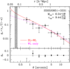
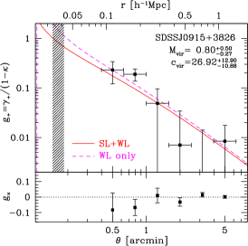
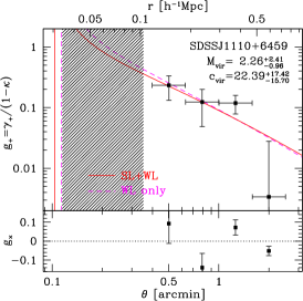
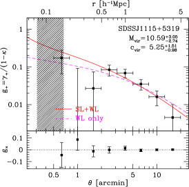
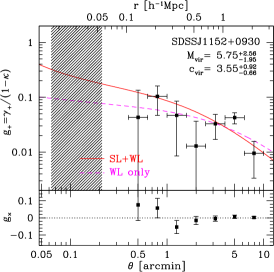
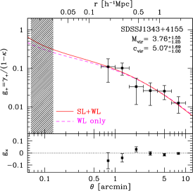
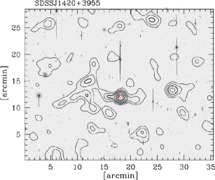
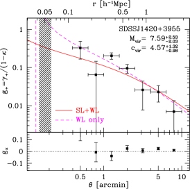
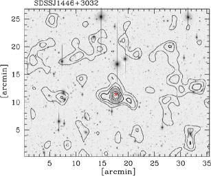
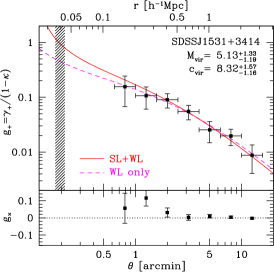
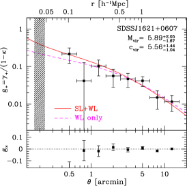
Table 3 summarizes our weak lensing analysis. It is seen that our PSF correction algorithm successfully reduces the stellar ellipticities to the level that are much smaller than typical lensing shear amplitudes for our cluster sample ($\gamma\ga 0.01$). The relatively small number density of $n_{g}\sim 10$ arcmin^-2 is due to the colour cut for selecting background galaxies. From the shear catalogues we compute tangential shear profiles. The tangential shear $g_{+}$ is computed from the reduced shear $\mbox{\boldmath$g$}=(g_{1},\,g_{2})$ as

$$g_{+}=-g_{1}\cos 2\phi-g_{2}\sin 2\phi,$$ (21)

where $\phi$ is the polar angle. Throughout the paper, we assume that the position of the brightest galaxy in the strong lensing region is coincident with the cluster centre. Although our strong lensing analysis suggests that the position of the mass peak can differ slightly from the central galaxy position, we find that any such offset is much smaller than the typical inner radial boundary of our weak lensing analysis. Hence the effect of off-centreing on our results should be negligibly small. The average shear value in each radial bin is estimated by the weighted mean of the tangential shear as follows:

$$\bar{g}_{+}=\left(\sum_{i}w_{g,i}g_{+,i}\right)\left(\sum_{i}w_{g,i}\right)^{-1},$$ (22)

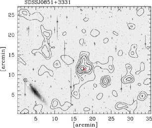
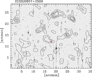
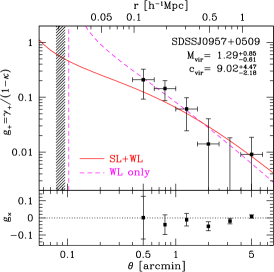
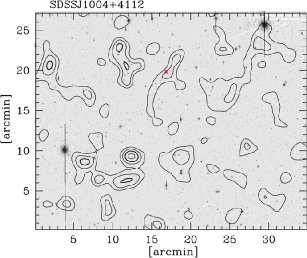
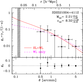
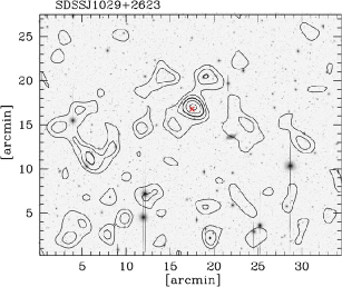
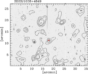
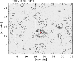
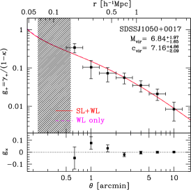
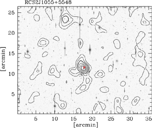
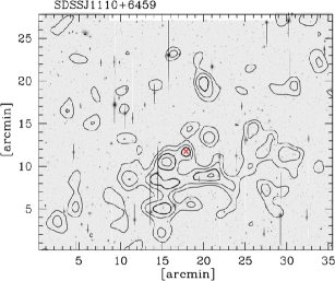
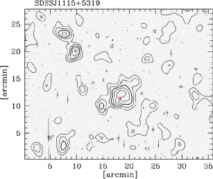
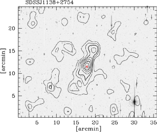
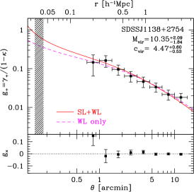
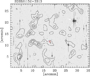
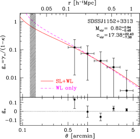
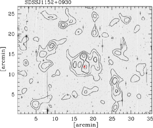
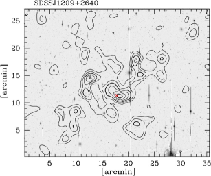
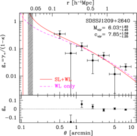
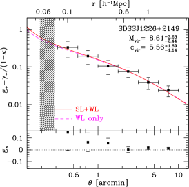
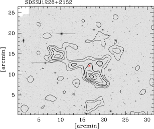
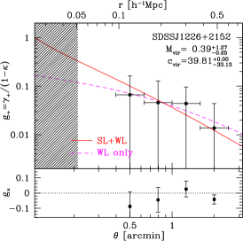
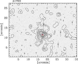
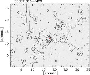
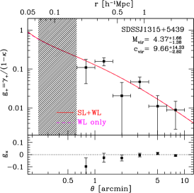
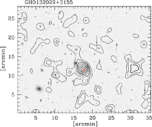
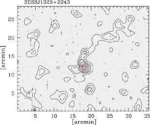
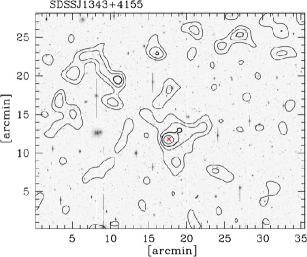
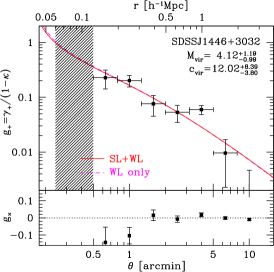
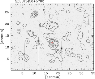
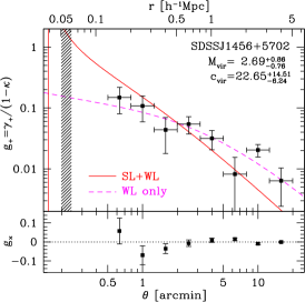
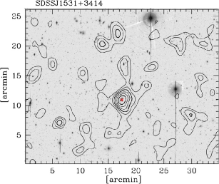
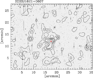
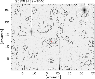
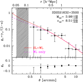
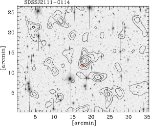
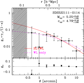
where the summation runs over all galaxies in the bin. Similarly the statistical error in the tangential shear measurement in each bin is computed from the weighted average of the variance of the shear, $\sigma_{g}^{2}$ (e.g., Okabe et al., 2010). The total signal-to-noise ratio of the tangential shear profile is shown in Table 3 and indicates that weak lensing signals are detected significantly ($S/N\ga 5$) for most of our clusters. The mass maps reconstructed from the weak lensing analysis are shown in Appendix B.

4 Combining strong and weak lensing

4.1 Methodology

We combine constraints from the tangential shear profile with constraints from strong lensing. As in Oguri et al. (2009), we combine both sets of constraints by summing up $\chi^{2}$:

$$\chi^{2}=\chi^{2}_{\rm SL}+\chi^{2}_{\rm WL}.$$ (23)

We include strong lensing constraints from the Einstein radius at the arc redshift:

$$\chi^{2}_{\rm SL}=\frac{\left[\bar{\theta}_{\rm E}-\theta_{\rm E}(M_{\rm vir},\,c_{\rm vir})\right]^{2}}{\sigma_{\rm E}^{2}},$$ (24)

where $\bar{\theta}_{\rm E}$ and $\sigma_{\rm E}$ are the best-fit Einstein radius at $z_{s}=z_{\rm arc}$ and its error presented in Table 2, and $\theta_{\rm E}(M_{\rm vir},\,c_{\rm vir})$ is the predicted Einstein radius assuming the NFW profile. On the other hand, weak lensing constraints come from binned tangential shear measurements:

$$\chi^{2}_{\rm WL}=\sum_{i}\frac{\left[\bar{g}_{+,i}-g_{+}(\theta_{i};\,M_{\rm vir},\,c_{\rm vir})\right]^{2}}{\sigma_{i}^{2}},$$ (25)

where $\bar{g}_{+,i}$ and $\sigma_{i}$ are observed reduced shear and its error at $i$-th radial bin, and $-g_{+}(\theta_{i};\,M_{\rm vir},\,c_{\rm vir})$ is the predicted reduced shear by the NFW model. The NFW profile, which we adopt as an analytical model for the radial mass distribution, has the three-dimensional density profile of

$$\rho(r)=\frac{\rho_{s}}{(r/r_{s})(1+r/r_{s})^{2}},$$ (26)

where

$$\rho_{s}=\frac{\Delta_{\rm vir}(z)\bar{\rho}_{m}(z)c_{\rm vir}^{3}}{3\left[\ln(1+c_{\rm vir})-c_{\rm vir}/(1+c_{\rm vir})\right]},$$ (27)

where $\Delta(z)$ is the nonlinear over-density predicted by the spherical collapse model. We parametrize the profile with two parameters, the virial mass $M_{\rm vir}$

$$M_{\rm vir}=\frac{4\pi}{3}r_{\rm vir}^{3}\Delta_{\rm vir}(z)\bar{\rho}_{m}(z),$$ (28)

and the concentration parameter $c_{\rm vir}$

$$c_{\rm vir}=\frac{r_{\rm vir}}{r_{s}}.$$ (29)

Figure 4: Correlation between strong and weak lensing observables. The best-fit mass $M_{\rm vir}$ for a fixed concentration of $c_{\rm vir}=6$ from just weak lensing is compared with the Einstein radius for the source redshift $z_{s}=2$ from strong lensing. The red line with shading shows the expected $M_{\rm vir}$-$\theta_{E}$ relation assuming the NFW profile with the concentration of $c_{\rm vir}=6\pm 2$.

4.2 Correlation between strong and weak lensing observables

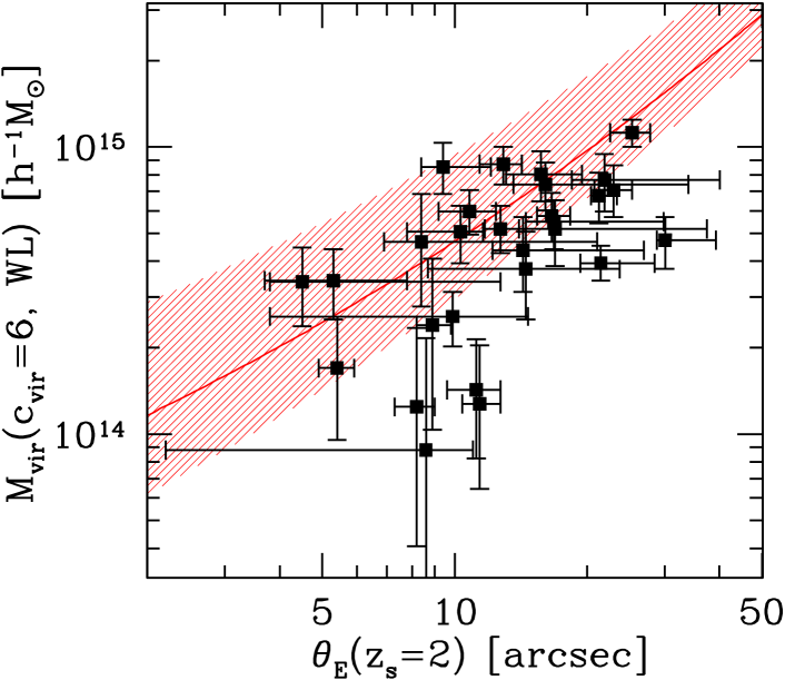
Before deriving best-fit parameters for individual clusters, we first compare strong and weak lensing observables, namely the Einstein radius and the virial mass, which should serve as a sanity check for results of more detailed analysis presented in the following sections. For the strong lensing observable, we use the Einstein radius for the fixed source redshift of $z_{s}=2$ in order to compare results for different clusters. Given the strong degeneracy between $M_{\rm vir}$ and $c_{\rm vir}$ in weak lensing analysis, we quantify the strength of the weak lensing signal by fitting the tangential shear profile for a fixed concentration parameter of $c_{\rm vir}=6$, a typical value for the concentration when the lensing selection effect is taken into account (see below). Figure 4 shows the correlation between the Einstein radius from strong lensing and the virial mass from weak lensing. We confirm that these two measurements are indeed correlated with each other such that the more massive clusters detected via their weak lensing have larger Einstein radii on average.

Assuming the NFW profile, the relation between mass and Einstein radius is determined by the concentration parameter. We also plot the expected correlation for the concentration assuming $c_{\rm vir}=6$, as well as the scatter of the relation originating from the shift of the concentration by $\pm 2$, for the lens redshift $z=0.46$ which corresponds to the median redshift of our cluster sample. We find that the observed correlation roughly follows the expectation for $c_{\rm vir}=6$, although there is a tendency for the Einstein radii to be larger than expected, particularly for low-mass clusters. This analysis suggests that our sample of clusters are slightly more concentrated than $c_{\rm vir}\sim 6$, and that clusters with lower masses on average have higher concentration values.

4.3 Fitting results

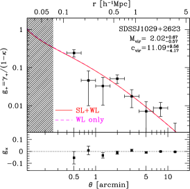
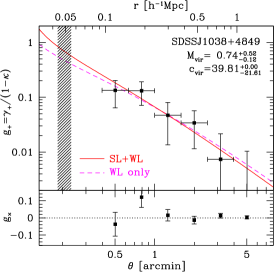
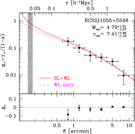
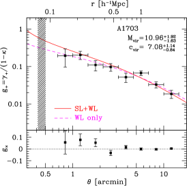
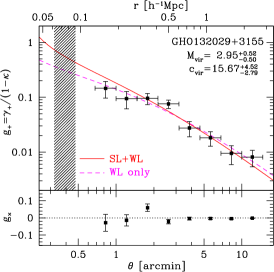
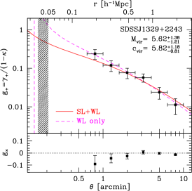
Table 4 summarizes the results of the combined analysis, i.e., simultaneous fitting of the observed Einstein radius and tangential shear profile with the NFW model predictions. The tangential shear profiles for individual clusters are compared with best-fit models in Appendix B. Fitting is performed in the parameter range $10^{13}h^{-1}M_{\odot}<M_{\rm vir}<10^{16}h^{-1}M_{\odot}$ and $0.01<c_{\rm vir}<39.81$. For four clusters studied previously in Oguri et al. (2009), our new results are fully consistent with the old result. In addition, the best-fit mass and concentration parameter for A1703 are in good agreement with the result of an independent strong and weak lensing analysis by Zitrin et al. (2010).

Table 4: Constraints on the mass $M_{\rm vir}$ and concentration parameter $c_{\rm vir}$ from weak lensing and combined strong and weak lensing analysis. Errors indicate $1\sigma$ errors on each parameter after marginalizing over the other parameter.

	Weak lensing					Strong and weak lensing
Name	$\chi^{2}$/dof	$M_{\rm vir}$	$c_{\rm vir}$	$M_{\rm vir}(c_{\rm vir}=6)$		$\chi^{2}$/dof	$M_{\rm vir}$	$c_{\rm vir}$
		($10^{14}h^{-1}M_{\odot}$)		($10^{14}h^{-1}M_{\odot}$)			($10^{14}h^{-1}M_{\odot}$)
SDSSJ0851+3331	4.2/7	$7.33^{+2.44}_{-1.96}$	$5.62^{+3.39}_{-2.03}$	$7.08^{+1.53}_{-1.39}$		5.8/8	$6.24^{+1.80}_{-1.61}$	$9.44^{+3.15}_{-1.85}$
SDSSJ0915+3826	7.0/6	$0.91^{+0.30}_{-0.28}$	$39.81^{+0.00}_{-17.16}$	$1.27^{+0.77}_{-0.63}$		8.0/7	$0.80^{+0.50}_{-0.27}$	$26.92^{+12.90}_{-10.88}$
SDSSJ0957+0509	1.2/6	$0.97^{+0.60}_{-0.31}$	$39.81^{+0.00}_{-27.65}$	$1.70^{+0.87}_{-0.74}$		2.9/7	$1.29^{+0.85}_{-0.61}$	$9.02^{+4.47}_{-2.18}$
SDSSJ1004+4112	0.8/6	$2.82^{+4.34}_{-1.92}$	$4.42^{+30.26}_{-3.74}$	$2.40^{+1.67}_{-1.36}$		1.0/7	$2.21^{+2.41}_{-1.43}$	$8.32^{+11.87}_{-3.13}$
SDSSJ1029+2623	9.7/8	$2.00^{+0.73}_{-0.60}$	$11.48^{+14.52}_{-5.02}$	$2.57^{+0.56}_{-0.55}$		9.7/9	$2.02^{+0.67}_{-0.57}$	$11.09^{+9.56}_{-4.17}$
SDSSJ1038+4849	1.2/6	$0.86^{+0.71}_{-0.39}$	$20.89^{+18.92}_{-13.56}$	$1.43^{+0.71}_{-0.61}$		1.4/7	$0.74^{+0.52}_{-0.12}$	$39.81^{+0.00}_{-21.61}$
SDSSJ1050+0017	3.2/7	$6.84^{+1.97}_{-1.71}$	$7.24^{+5.34}_{-2.67}$	$7.41^{+1.40}_{-1.39}$		3.2/8	$6.84^{+1.97}_{-1.65}$	$7.16^{+4.86}_{-2.09}$
RCS2J1055+5548	2.1/6	$5.13^{+1.71}_{-1.33}$	$6.17^{+4.07}_{-2.23}$	$5.19^{+1.05}_{-0.92}$		2.2/7	$4.79^{+1.31}_{-1.07}$	$7.41^{+1.40}_{-1.10}$
SDSSJ1110+6459	3.2/4	$2.07^{+2.15}_{-0.67}$	$35.89^{+3.92}_{-27.48}$	$4.68^{+2.16}_{-1.89}$		3.7/5	$2.26^{+2.41}_{-0.96}$	$22.39^{+17.42}_{-15.70}$
SDSSJ1115+5319	8.3/8	$11.61^{+3.52}_{-2.90}$	$2.66^{+1.23}_{-0.90}$	$7.67^{+1.77}_{-1.72}$		13.8/9	$10.59^{+3.05}_{-2.74}$	$5.25^{+1.51}_{-0.98}$
SDSSJ1138+2754	1.6/8	$11.22^{+2.58}_{-2.31}$	$3.55^{+1.52}_{-1.09}$	$8.71^{+1.29}_{-1.30}$		2.1/9	$10.35^{+2.09}_{-1.84}$	$4.47^{+0.60}_{-0.53}$
SDSSJ1152+3313	0.2/5	$0.73^{+1.33}_{-0.44}$	$27.54^{+12.27}_{-24.27}$	$1.24^{+1.10}_{-0.84}$		0.2/6	$0.82^{+0.94}_{-0.48}$	$17.38^{+22.43}_{-7.38}$
SDSSJ1152+0930	6.9/7	$7.24^{+3.59}_{-2.57}$	$1.66^{+1.33}_{-0.87}$	$3.39^{+1.08}_{-1.02}$		8.9/8	$5.75^{+2.56}_{-1.95}$	$3.55^{+0.92}_{-0.66}$
SDSSJ1209+2640	9.5/7	$6.92^{+2.52}_{-2.02}$	$5.75^{+3.69}_{-2.25}$	$6.76^{+1.37}_{-1.33}$		9.9/8	$6.03^{+1.83}_{-1.45}$	$7.85^{+1.59}_{-1.25}$
SDSSJ1226+2149	0.5/6	$8.81^{+3.63}_{-2.64}$	$5.25^{+2.51}_{-1.74}$	$8.04^{+1.63}_{-1.58}$		0.5/7	$8.61^{+3.28}_{-2.44}$	$5.56^{+1.69}_{-1.14}$
SDSSJ1226+2152	0.1/4	$0.80^{+75.05}_{-0.70}$	$6.84^{+32.97}_{-6.83}$	$0.88^{+1.28}_{-0.78}$		0.3/5	$0.39^{+1.27}_{-0.25}$	$39.81^{+0.00}_{-33.13}$
A1703	6.3/8	$12.88^{+2.61}_{-2.17}$	$4.79^{+1.24}_{-1.03}$	$11.22^{+1.22}_{-1.22}$		10.9/9	$10.96^{+1.92}_{-1.63}$	$7.08^{+1.14}_{-0.84}$
SDSSJ1315+5439	6.7/6	$4.42^{+1.82}_{-1.46}$	$9.44^{+15.97}_{-4.60}$	$5.19^{+1.34}_{-1.34}$		6.7/7	$4.37^{+1.66}_{-1.38}$	$9.66^{+14.33}_{-2.82}$
GHO132029+3155	5.3/8	$3.43^{+0.65}_{-0.58}$	$8.81^{+3.35}_{-2.35}$	$3.94^{+0.58}_{-0.51}$		9.7/9	$2.95^{+0.52}_{-0.50}$	$15.67^{+4.52}_{-2.79}$
SDSSJ1329+2243	1.1/6	$4.90^{+1.34}_{-1.14}$	$9.89^{+7.29}_{-3.58}$	$5.96^{+1.12}_{-1.00}$		2.7/7	$5.62^{+1.38}_{-1.21}$	$5.82^{+1.18}_{-0.81}$
SDSSJ1343+4155	1.8/6	$3.89^{+2.07}_{-1.46}$	$4.57^{+5.66}_{-2.33}$	$3.43^{+0.99}_{-0.92}$		1.9/7	$3.76^{+1.55}_{-1.25}$	$5.07^{+1.69}_{-1.00}$
SDSSJ1420+3955	8.9/7	$6.92^{+2.20}_{-1.79}$	$9.55^{+6.30}_{-3.31}$	$8.51^{+1.84}_{-1.67}$		13.5/8	$7.59^{+2.53}_{-2.03}$	$4.57^{+1.32}_{-0.98}$
SDSSJ1446+3032	14.8/7	$4.07^{+1.17}_{-0.98}$	$12.59^{+9.04}_{-4.37}$	$5.50^{+1.04}_{-1.08}$		14.9/8	$4.12^{+1.19}_{-0.99}$	$12.02^{+8.39}_{-3.80}$
SDSSJ1456+5702	7.6/8	$6.68^{+2.03}_{-1.67}$	$2.92^{+1.65}_{-1.16}$	$4.73^{+0.96}_{-0.97}$		21.4/9	$2.69^{+0.86}_{-0.76}$	$22.65^{+14.51}_{-6.24}$
SDSSJ1531+3414	0.6/7	$5.75^{+1.83}_{-1.44}$	$5.96^{+3.27}_{-2.07}$	$5.75^{+1.16}_{-1.08}$		1.3/8	$5.13^{+1.33}_{-1.19}$	$8.32^{+1.57}_{-1.16}$
SDSSJ1621+0607	2.6/8	$6.68^{+2.54}_{-2.01}$	$3.94^{+1.89}_{-1.39}$	$5.07^{+1.17}_{-1.13}$		3.8/9	$5.89^{+2.05}_{-1.67}$	$5.56^{+1.44}_{-1.04}$
SDSSJ1632+3500	2.7/7	$4.22^{+1.74}_{-1.40}$	$6.53^{+7.27}_{-3.06}$	$4.37^{+1.32}_{-1.24}$		2.9/8	$3.98^{+1.58}_{-1.26}$	$8.51^{+5.94}_{-2.05}$
SDSSJ2111$-$0114	2.2/7	$6.03^{+2.58}_{-2.14}$	$1.91^{+1.68}_{-1.01}$	$3.76^{+1.31}_{-1.25}$		6.0/8	$5.25^{+2.43}_{-1.94}$	$4.79^{+3.16}_{-1.62}$

With a large sample of clusters with measurements of the concentration parameter from combined strong and weak lensing, we can study the mass-concentration relation quite well. A caveat is that our sample of clusters are selected as those having prominent arcs. It has been noted that clusters selected by strong lensing (e.g., by giant arcs or large Einstein radii) represent a strongly biased population such that the concentration parameter inferred from the projected mass distribution is on average much larger mostly due to the halo triaxiality (Hennawi et al., 2007; Oguri & Blandford, 2009; Meneghetti et al., 2010). Although in Oguri et al. (2009) we assumed the constant enhancement of the concentration parameter due to the lensing bias, simple considerations suggest that the lensing bias of the mass-concentration relation should depend strongly on the mass. To derive more accurate theoretical predictions based on the $\Lambda$CDM model, in Appendix A we conduct a series of semi-analytic calculations with ray-tracing of extended sources to estimate the effect of the lensing bias, based on a triaxial halo model of Jing & Suto (2002). For reference, we find that the mean mass-concentration relation at $z=0.45$ with the lensing bias predicted by this model is roughly described by

$$\bar{c}_{\rm vir}(z=0.45)\approx 6.3\left(\frac{M_{\rm vir}}{5\times 10^{14}h^{-1}M_{\odot}}\right)^{-0.2},$$ (30)

which show relatively strong dependence on the halo mass, simply because of the mass dependence of the lensing bias (see Appendix A). The scatter of the relation is estimated to be $\sigma_{\log c}\simeq 0.12$.

Figure 5: The mass-concentration relation obtained from combined strong and weak lensing analysis. Filled triangles show our results presented in this paper, whereas filled squares show results from literature; A1689, A370, CL0024, RXJ1347 (Umetsu et al., 2011b), and A383 (Zitrin et al., 2011b). The black shaded region indicates the predicted concentration parameters as a function of the halo mass with the lensing bias taken into account (see Appendix A for details). The solid line is the best-fit mass-concentration relation from fitting of our cluster sample (i.e., filled triangles), with the 1$\sigma$ range indicated by dotted lines.

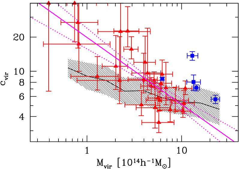
Figure 5 shows the mass-concentration relation obtained from our lensing analysis for 28 systems. For comparison, we also show accurate lensing measurements of the concentration parameters for 5 massive clusters from the literature (Umetsu et al., 2011b; Zitrin et al., 2011b). The Figure clearly indicates that measured concentrations are correlated well with the mass. More massive clusters have on average smaller concentrations, which is consistent with the theoretical expectation, although the slope is obviously much steeper.

To put this on a more quantitative footing, we fit the mass-concentration parameter with both the normalization and the mass slope as free parameters. Here we ignore the redshift dependence of the mass-concentration relation, given the predicted little evolution of the concentration of massive haloes with redshift (e.g., Zhao et al., 2009; Prada et al., 2011). We use the following estimator for fitting:

$$\chi^{2}=\frac{\left[\log\left(c_{\rm vir,obs}\right)-\log\left(c_{\rm vir,fit}\right)\right]^{2}}{\sigma_{\rm st}^{2}+\sigma_{\rm in}^{2}},$$ (31)

where $\sigma_{\rm st}$ is the $1\sigma$ measurement error on $\log(c_{\rm vir})$ for individual clusters from the lensing analysis (see Table 4), and $\sigma_{\rm in}=0.12$ is the intrinsic dispersion predicted by our calculations. We find that the best-fit mass-concentration relation from our lensing sample of 28 clusters is

$$\bar{c}_{\rm vir}=(7.7\pm 0.6)\left(\frac{M_{\rm vir}}{5\times 10^{14}h^{-1}M_{\odot}}\right)^{-0.59\pm 0.12},$$ (32)

where we also included $1\sigma$ errors on the normalization and the slope.

We detect a strong mass dependence of the concentration parameter with the slope of $-0.59\pm 0.12$ in our lensing sample, which should be compared with the predicted slope of $\approx-0.2$ for the strong lensing selected sample of clusters. We note that steeper mass-concentration relations than theoretical expectations were also suggested by previous weak lensing (Okabe et al., 2010) and X-ray (Schmidt & Allen, 2007; Buote et al., 2007; Ettori et al., 2010) analysis (see also Biviano, 2008). Our result suggests that the observed mass-concentration relation is in reasonable agreement with the simulation results for very massive haloes of $M_{\rm vir}\sim 10^{15}h^{-1}M_{\odot}$. The agreement may be even better if we adopt recent results of $N$-body simulations by Prada et al. (2011), who argued that previous simulation work underestimated the mean concentrations at high mass end (see also Appendix A). In contrast, we find that observed concentrations are much higher than theoretical expectations for less massive haloes of $M_{\rm vir}\sim 10^{14}h^{-1}M_{\odot}$, even if we take account of the mass dependence of the lensing bias.

A possible concern is the correlation of $M_{\rm vir}$ and $c_{\rm vir}$ for fitting of individual clusters which has been ignored in deriving the mass-concentration relation. We examine the possible effect of the degeneracy between $M_{\rm vir}$ and $c_{\rm vir}$ by the following Monte Carlo simulation. For each cluster, we change best-fit values of $M_{\rm vir}$ and $c_{\rm vir}$ by randomly picking up a point within the $1\sigma$ confidence region in the $M_{\rm vir}$-$c_{\rm vir}$ plane. After choosing new best-fit parameters for all the clusters, we re-fit the mass-concentration relation to derive best-fit values of the normalization and slope in equation (32). We repeat this simulation for 300 times to check how the correlated errors between $M_{\rm vir}$ and $c_{\rm vir}$ can affect our conclusion. We find that the resulting distribution of the best-fit normalization value is $7.6\pm 0.2$, and that of the slope is $-0.56\pm 0.05$, which are small compared with the statistical errors shown in equation (32), suggesting that the effect of the correlated error is not very significant. We note that Okabe et al. (2010) also explored potential impacts of the degeneracy between $M_{\rm vir}$ and $c_{\rm vir}$ on their mass-concentration measurement very carefully, and concluded that the effect is insignificant, which is consistent with our finding.

There are a few possible explanations for the excess concentration for small mass clusters. Perhaps the most significant effect is baryon cooling. The formation of the central galaxy, and the accompanying adiabatic contraction of dark matter distribution, enhances the core density of the cluster and increases the concentration parameter value for the total mass distribution. This effect is expected to be mass dependent such that lower mass haloes are affected more pronouncedly, simply because the fraction of the mass of the central galaxy to the total mass is larger for smaller halo masses. Indeed, simulations with radiative cooling and star formation indicate that the concentration can be significantly enhanced by baryon physics particularly for low-mass haloes (e.g., Rudd, Zentner, & Kravtsov, 2008; Mead et al., 2010), although the effect strongly depends on the efficiency of feedback (Duffy et al., 2010; McCarthy et al., 2010). Thus baryon cooling appears to be able to explain the observed strong mass dependence at least qualitatively. More quantitative estimates of this effect need to be made using a large sample of simulated clusters with the baryon physics as well as the proper feedback model included.

5 Stacking analysis

5.1 Stacked tangential shear profile

We can study the average properties of a given sample by stacking lensing signals. This stacked lensing analysis has been successful for constraining mean dark matter distributions of cluster samples (e.g., Mandelbaum et al., 2006b; Johnston et al., 2007; Leauthaud et al., 2010; Okabe et al., 2010). Here we conduct stacking analysis of the tangential shear profile for our lensing sample for studying the mass-concentration relation from another viewpoint. Note that the off-centreing effect, which has been known to be one of the most significant systematic errors in stacked lensing analysis (e.g., Johnston et al., 2007; Mandelbaum, Seljak, & Hirata, 2008; Oguri & Takada, 2011), should be negligible for our analysis, because of the detection of weak lensing signals for individual clusters and the presence of giant arcs which assure that selected centres (positions of the brightest galaxies in the strong lensing region) indeed correspond to that of the mass distribution.

We perform stacking in the physical length scale. Specifically, we compute the differential surface density $\Delta\Sigma_{+}(r)$ which is define by

$$\Delta\Sigma_{+}(r)\equiv\Sigma_{\rm cr}g_{+}(\theta=r/D_{ol}),$$ (33)

where $\Sigma_{\rm cr}$ is the critical surface mass density for lensing. We stack $\Delta\Sigma_{+}(r)$ for different clusters to obtain the average differential surface density. We do not include SDSSJ1226+2149 and SDSSJ1226+2152 in our stacking analysis, because these fields clearly have complicated mass distributions with two strong lensing cores separated by only $\sim 3^{\prime}$. Furthermore, we exclude SDSSJ1110+6459 as well because the two-dimensional weak lensing map suggests the presence of a very complicated mass distribution around the system. We use the remaining 25 clusters for our stacked lensing analysis.

Figure 6: The stacked tangential shear profile obtained by combining the 25 clusters. The average differential surface density $\langle\Delta\Sigma_{+}(r)\rangle$ (see equation 33) is plotted as a function of the physical radius $r$. Grey points indicate stacked tangential shear measurements from weak lensing that are not used for fitting. The upper left point with a horizontal error-bar is the constraint from the average Einstein radius. The solid line with shading is the best-fit NFW model with $1\sigma$ error range. The lower panel plots the stacked profile of the 45^∘ rotated component, $\langle\Delta\Sigma_{\times}(r)\rangle$.

It should be noted that the reduced shear $g_{+}$ has a non-linear dependence on the mass profile. In fact, the reduced shear is defined by $g_{+}\equiv\gamma_{+}/(1-\kappa)$, where $\gamma_{+}$ and $\kappa$ are tangential shear and convergence. Thus, the quantity defined by equation (33) still depends slightly on the source redshift via the factor $1/(1-\kappa)$, particularly near the halo centre. Thus, in comparison with the NFW predictions, we assume the source redshift of $z_{s}=1.1$, which is the typical effective source redshift for our weak lensing analysis (see Table 3). Also the non-linear dependence makes it somewhat difficult to interpret the average profile, and hence our stacked tangential profile measurement near the centre should be taken with caution.

It is known that the matter fluctuations along the line-of-sight contributes to the total error budget (e.g., Hoekstra, 2003; Hoekstra et al., 2011; Dodelson, 2004; Gruen et al., 2011). While we have ignored this effect for the analysis of individual clusters presented in Section 4, here we take into account the error from the large scale structure in fitting the stacked tangential shear profile by including the full covariance between different radial bins (see Oguri & Takada, 2011; Umetsu et al., 2011b, for the calculation of the covariance matrix). We, however, comment that the error of the large scale structure is subdominant in our analysis, because of the relatively small number density of background galaxies after the colour cut (see also Oguri et al., 2010).

In addition to weak lensing, we stack strong lensing constraints simply by averaging the Einstein radii for the fixed source redshift $z_{s}=2$. This constraint is combined with the stacked tangential shear profile from weak lensing to obtain constraints on the mass and concentration parameter for the stacked profile. Note that the Einstein radius is related with the reduced shear as $g_{+}(\theta_{\rm E})=1$. Given the uncertainty from the non-linearity of the reduced shear and the the possible bias coming from the uncertainty of the outer mass profile (Oguri & Hamana, 2011; Becker & Kravtsov, 2011), we restrict tangential shear fitting in the range $0.158h^{-1}{\rm Mpc}<r<3.16h^{-1}{\rm Mpc}$. However we note that our results are not largely changed even if we conduct fitting in the whole radius range.

Figure 7: Similar to Figure 6, but the stacked lensing analysis in three $\theta_{\rm E}$ bins is presented. From top to bottom, results for largest to smallest $\theta_{\rm E}$ bins are shown. Curves and points for the largest and smallest $\theta_{\rm E}$ bins are shifted vertically by $\pm 0.5$ dex respectively for illustrative purposes.

Figure 8: Same as Figure 7, but clusters are binned in $M_{\rm vir}$.

Table 5: Summary of stacked tangential shear analysis

Sample	$N$	$\langle z\rangle$	$\langle\theta_{\rm E}\rangle$	$\langle M_{\rm vir}\rangle$	$\langle c_{\rm vir}\rangle$
			(arcsec)	($10^{14}h^{-1}M_{\odot}$)
all	25	0.469	$14.4^{+10.6}_{-7.0}$	$4.57^{+0.33}_{-0.31}$	$5.75^{+0.70}_{-0.57}$
$\theta_{\rm E}$-1	4	0.379	$22.8^{+4.3}_{-2.8}$	$6.03^{+0.74}_{-0.72}$	$7.94^{+1.28}_{-1.02}$
$\theta_{\rm E}$-2	5	0.416	$13.0^{+2.4}_{-2.8}$	$3.13^{+0.50}_{-0.50}$	$10.23^{+2.65}_{-1.82}$
$\theta_{\rm E}$-3	7	0.471	$8.3^{+2.6}_{-2.4}$	$3.51^{+0.52}_{-0.52}$	$7.08^{+1.53}_{-1.12}$
$M_{\rm vir}$-1	5	0.480	$17.1^{+12.9}_{-6.4}$	$9.55^{+1.17}_{-1.04}$	$4.90^{+0.79}_{-0.73}$
$M_{\rm vir}$-2	10	0.472	$14.7^{+10.2}_{-5.7}$	$5.62^{+0.61}_{-0.55}$	$5.37^{+0.87}_{-0.75}$
$M_{\rm vir}$-3	10	0.460	$12.6^{+9.3}_{-7.8}$	$1.97^{+0.32}_{-0.29}$	$10.59^{+4.54}_{-2.83}$

Figure 9: The mass-concentration relation obtained from the stacked lensing analysis. We show stacking results of 3 $\theta_{\rm E}$ bins (filled squares) and 3 $M_{\rm vir}$ bins (open circles). The mass and concentration measured from stacked strong and weak lensing analysis of 4 massive clusters at $z\sim 0.32$ (Umetsu et al., 2011b) are indicated by a cross. The black shading region shows theoretically expected mass-concentration relations with the lensing bias (see Appendix A for details). The solid and dotted lines are bets-fit relation from individual analysis shown in Figure 5.

Figure 10: Concentration parameters from stacking lensing analysis as a function of the Einstein radius for the source redshift $z_{s}=2$. The black shading region indicates the theoretical expectation with the selection effect (see Appendix A for details). Symbols are same as Figure 9.

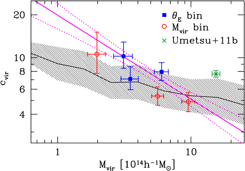
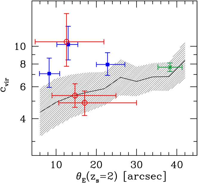
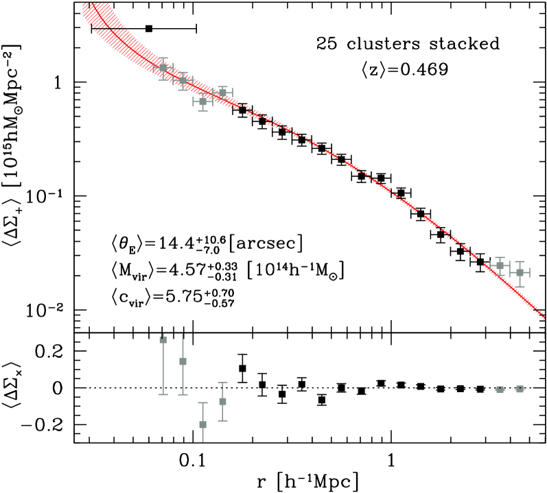
Figure 6 shows the stacking result for all the 25 clusters. The mean cluster redshift for this sample is $\langle z\rangle=0.469$. The total signal-to-noise ratio in the whole radius range of $0.063h^{-1}{\rm Mpc}<r<5.01h^{-1}{\rm Mpc}$ is $S/N=32$. We find that stacked tangential shear profile from weak lensing is fitted well by the NFW profile over a wide range in radius. The average Einstein radius from strong lensing ($\langle\theta_{\rm E}\rangle=14\aas@@fstack{\prime\prime}4^{+10.6}_{-7.0}$) is slightly larger than the best-fit model predicts ($\theta_{\rm E}=9\aas@@fstack{\prime\prime}1$), although they are consistent with each other well within $1\sigma$. The best-fit mass and concentration are $\langle M_{\rm vir}\rangle=4.57^{+0.33}_{-0.31}\times 10^{14}h^{-1}M_{\odot}$ and $\langle c_{\rm vir}\rangle=5.75^{+0.70}_{-0.57}$. We note that the mean mass measured by the stacking analysis agrees well with the mean mass of strong lens selected clusters predicted by ray-tracing simulations, $\langle M_{\rm vir}\rangle\sim 4.2\times 10^{14}h^{-1}M_{\odot}$ (Hennawi et al., 2007, see also Bayliss et al. 2011b).

The concentration parameter measured in the stacked tangential shear profile is broadly consistent with the result of individual analysis (see Figure 5), but appears to be slightly smaller than the mass-concentration relation constrained from our lensing sample. Here we estimate the impact of the possible averaging effect by computing an average shear profile from reduced shear profiles of the NFW profile with best-fit values of the mass and concentration from individual cluster analysis (Table 4), and comparing it with the reduced shear profile of the NFW profile with the median values of the mass and concentration. We find that both profiles agree well near the virial radius, but the averaged profile underestimates the shear profile toward the centre, with $\sim 10\%$ systematic difference at around $0.2h^{-1}$Mpc. Both the profiles agree well again at the innermost radii of $<0.1h^{-1}$Mpc down to the strong lensing region. The systematic difference translates into the concentration parameter of $\Delta c_{\rm vir}\sim-1.2$, and hence it can partly explain the smaller concentration parameter value from the stacked lensing analysis.

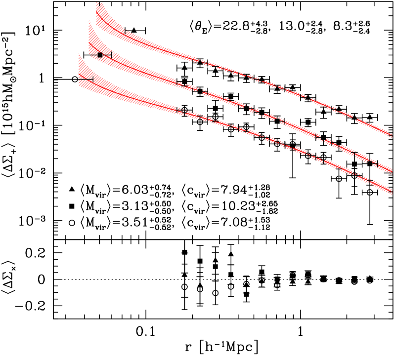
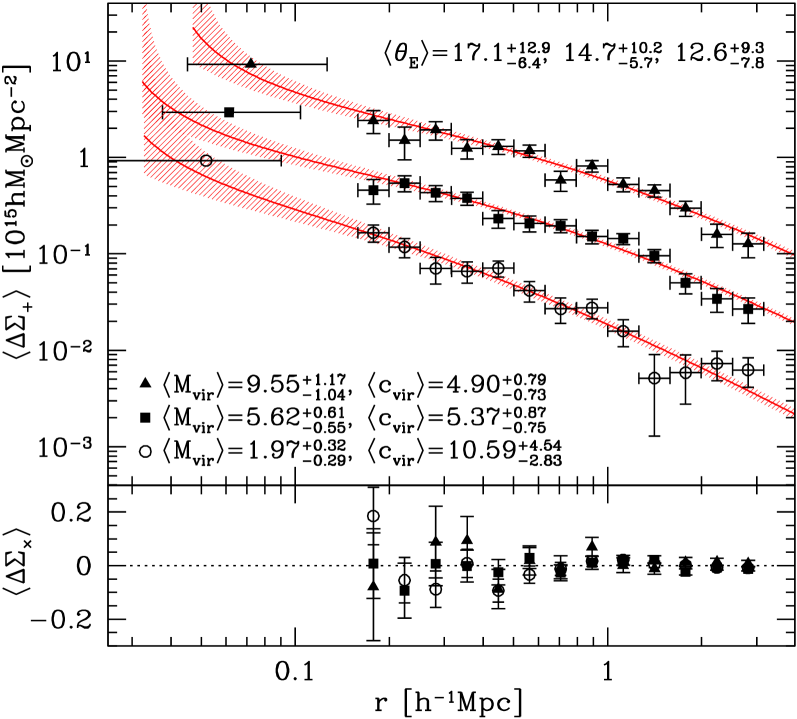
Another possible reason for the smaller concentration from the stacked tangential shear is a wide range of $\theta_{\rm E}$ of our sample, which results in the large error on the mean Einstein radius and therefore in the much weaker constraints from strong lensing compared with individual modelling cases. Hence, we conduct the same stacking analysis by dividing our cluster sample into 3 $\theta_{\rm E}$ bins. In order to assure reasonable constraints from strong lensing, we remove 9 clusters which have large errors on $\theta_{\rm E}$ mostly because of the lack of arc redshift information. To test the mass dependence of the concentration, in addition to $\theta_{\rm E}$ bins we consider 3 $M_{\rm vir}$ bins too. We use all the 25 clusters for the mass bin analysis.

Results of our stacking analysis in different $\theta_{\rm E}$ and $M_{\rm vir}$ bins are shown in Figures 7 and 8, respectively, and are summarized in Table 5. We find that clusters in the largest $\theta_{\rm E}$ bin are indeed most massive. However, the second and third $\theta_{\rm E}$ bins have similar mean virial masses, and the difference of the Einstein radii appear to be derived by the different concentrations. On the other hand, different mass bins have similar Einstein radii, but the concentrations are clearly larger for smaller masses.

These results can be used to check the mass-concentration relation inferred from individual analysis of clusters. Figure 9 shows the mass-concentration relation similar to Figure 5, but this time the relation obtained from stacked lensing analysis. We find that the mass-concentration relation from stacking analysis is in reasonable agreement with the best-fit relation constrained from individual analysis of strong and weak lensing (equation 32). In particular, the strong mass dependence of the concentration is clearly seen in the stacking analysis as well. The slightly smaller normalization compared with individual analysis can partly be ascribed to the averaging effect as described above. Thus the stacking analysis further confirms the measurement of the mass-concentration relation from our sample of clusters.

In Figure 10 we study the dependence of concentration parameters derived from the stacking analysis with the Einstein radius. In particular we compare it with semi-analytic calculation conducted in Appendix A which predicts that the clusters with larger Einstein radii are more concentrated. While it is hard to see this trend in our cluster sample, we find that the high concentration of massive lensing clusters presented by Umetsu et al. (2011b) can be explained in this context. Our result suggests that the average concentration of the Umetsu et al. (2011b) cluster sample is in good agreement with the theoretical expectation given the very large Einstein radii of $\theta_{\rm E}\sim 40^{\prime\prime}$.

Figure 11: The two-dimensional weak lensing shear maps obtained from stacking analysis of 25 clusters. The sticks shows observed directions and strengths of weak lensing shear distortion. Colour contours are the surface density map reconstructed from the shear map using the standard inversion technique (Kaiser & Squires, 1993). Both the shear and density maps are smoothed for illustrative purpose. Left: The result when the position angle of each cluster is aligned to the North-South axis before stacking, by using the position angle measured in strong lens modelling. The resulting stacked density distribution is clearly elongated along the North-South direction. Right: The result without any alignment of the position angle when stacking. The resulting density distribution is nearly circular symmetric in this case.

5.2 Two-dimensional stacking analysis

In addition to stacking of the tangential shear profile, we conduct stacking of two-dimensional (2D) shear maps to study the mean shape of the projected dark matter distribution in clusters. Such 2D stacking analysis has been attempted for samples of galaxies (Natarajan & Refregier, 2000; Hoekstra et al., 2004; Mandelbaum et al., 2006a; Parker et al., 2007) or for clusters (Evans & Bridle, 2009). The biggest problem of these 2D stacking analysis has been that the position angle (orientation) of the projected mass distribution has to be known for each cluster when stacking. In previous work it was assumed that the position angle of the mass distribution coincides with that of the light distribution, e.g., the surface brightness distribution of the central or satellite galaxy distributions, although the assumption has not yet been fully justified (Oguri et al., 2010; Bett, 2011).

Our unique sample of strong and weak lensing clusters provides an important means of overcoming this difficulty. The idea is that strong lens modelling can generally constrain the position angle of the dark halo component quite well, which can be used as a prior information for the position angle to stack weak lensing signals. This procedure evades any assumptions on the alignment between mass and light, and hence should enable much more robust 2D stacking analysis.

As in Section 5.1, we conduct stacking analysis in the physical length scale. For each cluster, we adopt the position angle obtained in strong lens mass modelling ($\theta_{e}$ in Table 2) to rotate the catalogue of the background galaxies by $-\theta_{e}$ such that the the position angle of the dark halo is aligned with the North-South axis. Specifically, the position of a galaxy at ($x$, $y$) with respect to the cluster centre is changed to

$$x^{\prime} = x\cos\theta_{e}+y\sin\theta_{e},$$ (34)

$$y^{\prime} = -x\sin\theta_{e}+y\cos\theta_{e},$$ (35)

and the two shear components ($g_{1}$, $g_{2}$) are modified as

$$g_{1}^{\prime} = g_{1}\cos 2\theta_{e}+g_{2}\sin 2\theta_{e},$$ (36)

$$g_{2}^{\prime} = -g_{1}\sin 2\theta_{e}+g_{2}\cos 2\theta_{e}.$$ (37)

We stack the rotated shear catalogue in the physical unit, $\Sigma_{\rm cr}\mbox{\boldmath$g$}^{\prime}(\mbox{\boldmath$r$}^{\prime})$, to obtain the average 2D shear map of our cluster catalogue. The cluster catalogues analyzed in this section is same as those in Section 5.1, containing 25 clusters in total.

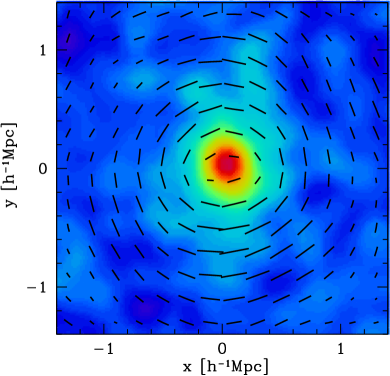
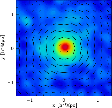
The stacked 2D shear map, as well as the corresponding density map reconstructed from the shear map, are shown in Figure 11. As expected, the projected mass distribution from the stacked 2D shear map is quite elongated along the North-South direction, suggesting the highly elongated mass distribution of our cluster sample. As a sanity check, we also compute the 2D shear map without any alignment of the position angle when stacking. The resulting mass distribution shown in Figure 11 appears to be circular symmetric, which supports that the highly elongated distribution in our stacked map is not an artifact.

We constrain the ellipticity of the projected 2D mass distribution by directly fitting the 2D shear map with the elliptical NFW model prediction. Here we closely follow the procedure detailed in Oguri et al. (2010) for the 2D shear fitting. Briefly, we modify the convergence $\kappa(r)$ (i.e., the projected surface mass density) of the spherical NFW profile simply by introducing the ellipticity in the iso-density contour as $r^{2}\rightarrow x^{2}/(1-e)+y^{2}(1-e)$. With this procedure our definition of the ellipticity is $e=1-b/a$, where $a$ and $b$ are major and minor axis lengths of the isodensity contour. The corresponding shear pattern is computed by solving the Poisson equation. We then construct pixelized distortion field by computing mean shear and errors in each bin, and compare it with the elliptical model prediction, adopting the pixel size of $0.1h^{-1}{\rm Mpc}$. We add the contribution of the large scale structure to the error covariance matrix (see Oguri et al., 2010). We perform fitting in a $6h^{-1}{\rm Mpc}\times 6h^{-1}{\rm Mpc}$ region, but remove the innermost $4\times 4$ pixels considering several possible systematics that might be affecting signals near the centre. Unlike Oguri et al. (2010), we fix the mass centre to the assumed centre (the position of the brightest galaxy in strong lensing region), because strong lensing available for our cluster sample allows a reliable identification of the mass centre for each cluster. Thus we fit the 2D shear map with four parameters ($M_{\rm vir}$, $c_{\rm vir}$, $e$, $\theta_{e}$), employing a Markov Chain Monte Carlo technique.

Figure 12: The marginalized probability distribution of the mean ellipticity $\langle e\rangle$ from stacked weak lensing analysis of 25 clusters. The solid line indicates the case when the position angles are aligned according to those measured with strong lens modelling, in which the mean ellipticity is detected at $5\sigma$ level ($\langle e\rangle=0.47\pm 0.06$). The dashed line is the marginalized probability distribution for stacking without any alignment of the position angles, for which the mass distribution is consistent with the circular symmetric distribution ($\langle e\rangle<0.19$). The vertical dotted line indicates the theoretical expectation, $\langle e\rangle=0.44$, based on a triaxial halo model of Jing & Suto (2002). The open circle with errorbar shows the average ellipticity and $1\sigma$ scatter from strong lens modelling.

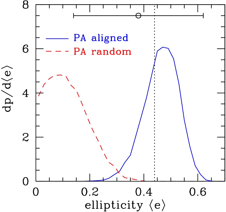
In Figure 12, we show the posterior likelihood distribution of the mean ellipticity $\langle e\rangle$ from the 2D stacking analysis of all the 25 clusters. When the position angles are aligned, the resulting density distribution is indeed quite elliptical with the mean ellipticity of $\langle e\rangle=0.47\pm 0.06$. We find that the elliptical NFW model improve fitting by $\Delta\chi^{2}=26.9$ compared with the case $e=0$, which indicates that the detection of the elliptical mass distribution is significant at the $5\sigma$ level. The measured mean ellipticity is consistent with the average ellipticity from strong lens modelling $\langle e\rangle=0.38\pm 0.24$, although the latter involves large scatter. The best-fit position angle of $\theta_{e}=9.1^{+3.9}_{-4.1}$ deg slightly deviates from the expected position angle of $\theta_{e}=0$, but they are consistent with each other within $2\sigma$ ($\Delta\chi^{2}<4$). In contrast, if the position angles are not aligned in stacking shear signals, the resulting constraint on the mean ellipticity is $\langle e\rangle<0.19$, i.e., it is fully consistent with the circular symmetric mass distribution $e=0$ within $1\sigma$.

Figure 13: The mean ellipticities measured in stacked 2D shear map as a function of the box size for fitting. Our fiducial result and its $1\sigma$ range adopting half the box size of $3h^{-1}{\rm Mpc}$ are indicated by the horizontal line with shading.

We compare this result with the theoretical prediction in the $\Lambda$CDM model. For this purpose we employ a triaxial model of Jing & Suto (2002). Assuming that the halo orientation is random, we compute the probability distribution of the ellipticity by projecting the triaxial halo along arbitrary directions (Oguri et al., 2003; Oguri & Keeton, 2004). In this analysis we fix the mass and redshift of the halo to $M_{\rm vir}=4.6\times 10^{14}h^{-1}M_{\odot}$ and $z=0.469$, which are mean mass and redshift of the 25 clusters. We find that the mean ellipticity predicted by this model is $\langle e\rangle=0.44$, in excellent agreement with the measured ellipticity. The analysis presented in Appendix A indicates that the effect of the lensing bias on the mean ellipticity is small, with a possible shift of the mean ellipticity of $\la 0.05$ at most, and hence it does not affect our conclusion. Our result is also in good agreement with the previous lensing measurement of the ellipticity by Oguri et al. (2010) in which 2D shear maps of individual clusters are fitted with the elliptical NFW profile, rather than examining the stacked shear map.

Figure 14: Mean ellipticities from stacked shear maps in three different $\theta_{\rm E}$ (upper panel) and $M_{\rm vir}$ (lower panel) bins. The horizontal line with shading indicate best-fit and 1$\sigma$ range of the full sample result. Dashed lines show the predicted mean ellipticity from semi-analytic calculations with the lensing bias (see Appendix A for details).

Table 6: Summary of the two-dimensional stacking analysis

Sample	$\langle e\rangle$	$\langle\theta_{e}\rangle$
		(deg)
all	$0.47^{+0.06}_{-0.06}$	$9.1^{+3.9}_{-4.1}$
$\theta_{\rm E}$-1	$0.29^{+0.13}_{-0.18}$	$14.1^{+13.9}_{-18.8}$
$\theta_{\rm E}$-2	$0.70^{+0.05}_{-0.09}$	$13.0^{+4.4}_{-4.3}$
$\theta_{\rm E}$-3	$0.52^{+0.10}_{-0.14}$	$6.7^{+12.2}_{-9.2}$
$M_{\rm vir}$-1	$0.58^{+0.04}_{-0.09}$	$5.2^{+4.4}_{-4.5}$
$M_{\rm vir}$-2	$0.28^{+0.12}_{-0.14}$	$9.7^{+11.3}_{-17.6}$
$M_{\rm vir}$-3	$0.60^{+0.09}_{-0.11}$	$16.7^{+7.0}_{-8.7}$

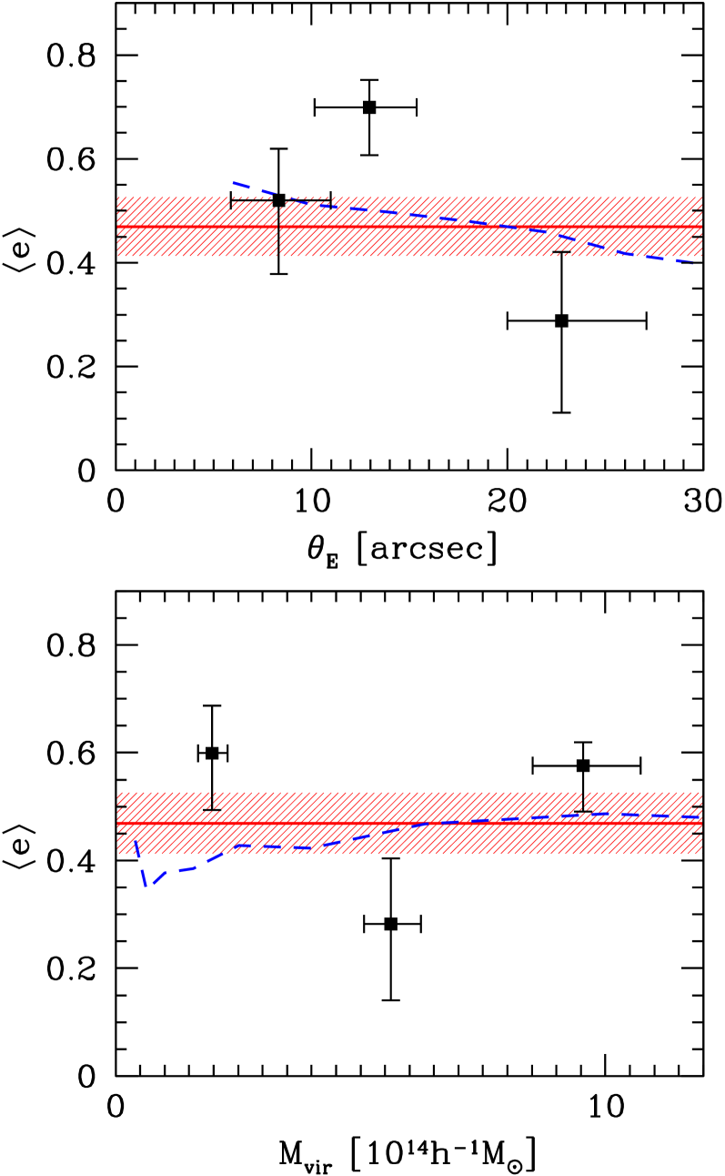
We check the sensitivity of our ellipticity result on the size of the fitting region, as one possible concern is that infalling matter associated with the filamentary structure outside clusters might boost the mean ellipticity. Figure 13 shows how the constraint on the mean ellipticity changes by making the size of the fitting region smaller from our fiducial choice (half the box size of $3h^{-1}{\rm Mpc}$). The Figure indicates that the detection of the mean ellipticity of $\sim 0.45$ is robust against the choice of the fitting size, as the results are consistent down to half the box size of $\sim 0.3h^{-1}{\rm Mpc}$ where the constraint become significantly weak. The analysis also implies that the ellipticity of the projected mass distribution does not change very much with radius. Theoretically, dark haloes are expected to be more elongated near the centre (Jing & Suto, 2002), although the effect of baryon cooling and star formation can make the shape rounder particularly near the centre (Kazantzidis et al., 2004; Lau et al., 2011). Our detection of the elliptical mass distribution down to small radii may therefore help constraining the amount of cooling in clusters.

Finally we check the mean ellipticities for different $\theta_{\rm E}$ and $M_{\rm vir}$ bins. Figure 14 shows the results, and Table 6 gives the summary of constraints on the mean ellipticities. We find a possible decrease of $\langle e\rangle$ at the largest Einstein radius bin, although it is not very significant given the large errorbars. On the other hand, there appears no simple trend in the mass bin result.

While results for all subsamples are almost consistent with the full sample result, the dependence on $\theta_{\rm E}$ might be suggestive of conflicting selection effects on our sample. There are two main lensing biases that can affect the results on the mean ellipticity measurement. One is the orientation bias, i.e., clusters with larger Einstein radii appear to be rounder than normal clusters because of the alignment of the major axis with the line-of-sight direction (Oguri & Blandford, 2009). The other selection effect is directly related to the ellipticity of the projected mass distribution. Because the ellipticity significantly enhances the giant arc cross section (e.g., Meneghetti, Bartelmann, & Moscardini, 2003; Meneghetti et al., 2007), a sample of clusters with prominent lensed arcs should have more elliptical projected mass distribution. These two selection effects apparently conflict with each other, although a naive expectation is that the orientation bias dominates for large Einstein radii, whereas the ellipticity bias is more significant for small Einstein radii. Indeed, our semi-analytic calculations presented in Appendix A shows a clear dependence of the mean ellipticity on the Einstein radius, as plotted in Figure 14. The observed trend appears to be consistent, at least qualitatively, with the theoretical prediction. A large sample is needed to confirm this trend more robustly.

6 Relation between mass and member galaxy distributions

Understanding the relation between the mass and cluster member galaxy distributions is important for the cosmological use of optical clusters (e.g., Koester et al., 2007; Rozo et al., 2009, 2011; Rykoff et al., 2011) as well as detailed stacking analysis for a large sample of clusters (e.g., Evans & Bridle, 2009). The spatial distribution of galaxies, in comparison with that of subhaloes in an $N$-body simulation, is crucial for exploring the formation history of cluster member galaxies (e.g., Nagai & Kravtsov, 2005). Here we examine spatial distributions of cluster member galaxies using the stacking technique, and compare them with accurate measurements of mass distributions from stacked lensing analysis.

While the colour information from $gri$-band images allows us to select the galaxy population around a given redshift efficiently, the selection is not perfect in the sense that there is some contamination from foreground and background galaxies. Thus, in this paper we take advantage of the high number density of galaxies after stacking to subtract the foreground and background galaxies statistically. Specifically, we assume that the stacked number density distribution is described by the sum of cluster member galaxies and background galaxies as:

$$\Sigma_{g}(\mbox{\boldmath$r$})=a_{g}\Sigma_{\rm nfw}(\mbox{\boldmath$r$})+b_{g},$$ (38)

where $a_{g}$ is the normalization, $\Sigma_{\rm nfw}$ is the surface density distribution of the NFW profile, and $b_{g}$ is the number density of foreground/background galaxies which is assumed to be constant across the field.

In this paper, we focus on two parameters that describe the number density distribution of member galaxies. One is the scale radius $r_{s}$ of the NFW profile, which is used to check whether or not the galaxy distribution is more extended than the mass distribution. The other is the ellipticity of the projected number density distribution, as our stacking analysis enables detailed analysis of 2D distributions for both mass and member galaxy distributions. We constrain the scale radius $r_{s}$ by fitting azimuthally averaged radial profile of the galaxy number density, whereas the ellipticity is derived from the 2D fitting of the density distribution. The total number of parameters for the radial profile fitting is 3 ($r_{s}$, $a_{g}$, and $b_{g}$), and the that of 2D fitting is 5 ($e$, $\theta_{e}$, $r_{s}$, $a_{g}$, and $b_{g}$).

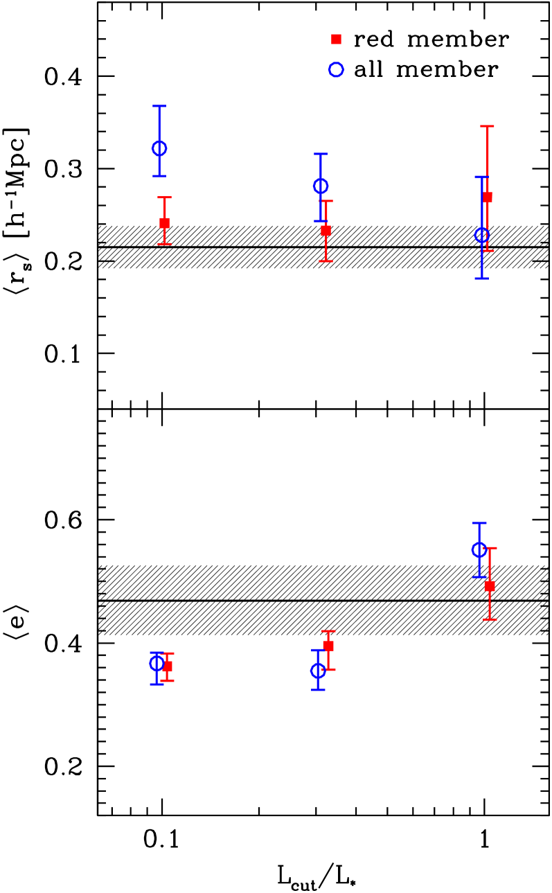
We consider two distinct galaxy populations, one is red member galaxies selected by the colour cut (equations 7 and 8), and the other is all galaxies without any colour cut. For each galaxy population, we consider galaxies that are more luminous than the luminosity cut, i.e., $L>L_{\rm cut}$. The luminosity cut is defined in terms of $L_{*}$, where $L_{*}$ is the luminosity corresponding to the $i$-band absolute magnitude $M_{*}^{i}=-21.22+5\log h$ (Rykoff et al., 2011). For the highest cluster redshift in our sample, a luminosity $0.1L_{*}$ corresponds to $i\sim 24.5$, which is well above the magnitude limit of our Subaru imaging.

Figure 15: The mean scale radius $\langle r_{s}\rangle$ (upper) and mean ellipticity $\langle e\rangle$ (lower) of the member galaxy distribution from stacking 25 clusters, as a function of the luminosity cut $L_{\rm cut}$. Filled squares and open circles show the results for red member galaxies and all member galaxies, respectively. Horizontal lines with shading are the scale radius and ellipticity for the mass distribution, measured by stacked lensing, for the same cluster sample.

Table 7: analysis results on the member galaxy distribution

$L_{\rm lim}$	$\langle r_{s}\rangle$ (red)	$\langle e\rangle$ (red)	$\langle r_{s}\rangle$ (all)	$\langle e\rangle$ (all)
($L_{*}$)	($h^{-1}{\rm Mpc}$)		($h^{-1}{\rm Mpc}$)
1	$0.27^{+0.08}_{-0.06}$	$0.49^{+0.06}_{-0.05}$	$0.23^{+0.06}_{-0.05}$	$0.55^{+0.04}_{-0.04}$
$10^{-0.5}$	$0.23^{+0.03}_{-0.03}$	$0.40^{+0.02}_{-0.04}$	$0.28^{+0.04}_{-0.04}$	$0.36^{+0.03}_{-0.03}$
$10^{-1}$	$0.24^{+0.03}_{-0.02}$	$0.36^{+0.02}_{-0.02}$	$0.32^{+0.05}_{-0.03}$	$0.37^{+0.02}_{-0.03}$

We show our fitting results in Figure 15 and Table 7. We find that the mass and galaxy number distributions agree reasonably well for the luminous galaxies, $L\ga L_{*}$, for both the scale radius and ellipticity. However, for fainter galaxies of $L\sim 0.1L_{*}$ the scale radius of the galaxy distribution tends to be larger (i.e., smaller concentration parameter values), and the average ellipticity is smaller.

The radial distribution has also been studied in previous work. Measurements of the projected number density distributions suggest low concentration values of $c\sim 2-5$ (Lin, Mohr, & Stanford, 2004; Katgert et al., 2004; Hansen et al., 2005; Lin & Mohr, 2007; Biviano & Poggianti, 2009). Lin & Mohr (2007) found that more luminous galaxies tend to be distributed with large concentrations, which is consistent with our results in Figure 15. Simulation work by Nagai & Kravtsov (2005) also predicts that the galaxy number density distribution is slightly more extended than the mass distribution, which is again consistent with our result, although no significant dependence of the concentration on the stellar mass was reported from the simulations.

There have been measurements of the ellipticity of the projected galaxy number density distributions (e.g., Paz et al., 2006; Niederste-Ostholt et al., 2010), but its connection with the underlying mass distribution has not yet fully been explored. The similar ellipticity for luminous member galaxies is reasonable, but the origin of the smaller mean ellipticity for fainter galaxies is unclear. Essentially, the smaller mean ellipticity for the stacked cluster sample indicates either the galaxy distribution is on average rounder or there is a large misalignment (i.e., difference in the position angles) between the mass and galaxy distribution. In either case careful simulation work is crucial to check if the observed distribution is in agreement with current understanding of cluster galaxy formation.

7 Conclusion

We have performed a combined strong and weak lensing analysis for a sample of 28 clusters in the redshift range $0.28<z<0.68$. The cluster sample is based on the SGAS, a large survey of giant arcs amongst SDSS clusters. In this paper, we have presented extensive follow-up observations with Subaru/Suprime-cam, which enables reliable weak lensing measurements out to large radii. Combined with the giant arcs with significant amount of spectroscopic information, we can constrain mass distributions of these clusters quite well to measure the concentration and shape of the mass distribution.

The mass-concentration relation derived from our lensing analysis has the slope of $c_{\rm vir}\propto M_{\rm vir}^{-0.59\pm 0.12}$, which is significantly steeper than the slope predicted by the theoretical expectation of $-0.2$ which includes the effect of the lensing bias. Concentrations measured by the combined lensing analysis are in reasonable agreement with the $\Lambda$CDM prediction for massive clusters ($M_{\rm vir}\sim 10^{15}h^{-1}M_{\odot}$), if we take proper account of the lensing bias. The result indicates that the anomalously high concentration (Broadhurst et al., 2005, 2008; Oguri et al., 2009; Umetsu et al., 2011b; Gralla et al., 2011), which has been claimed from analysis of small number of lensing clusters, is now much less evident, thanks to the much larger number of clusters we have analyzed in the paper. On the other hand, observed concentrations appear to be significantly higher than theoretical expectations for lower masses of $M_{\rm vir}\sim 10^{14}h^{-1}M_{\odot}$, which may be explained as arising from the effects of cooling baryons in cluster centres.

We have also stacked tangential shear profiles for the sample of clusters to obtain an accurate mean profile, which is seen to be in good agreement with the NFW profile. Our stacking analysis at different Einstein radii and mass bins has confirmed our results on the mass-concentration relation from the individual analysis of these clusters. In addition to the radial profile, we have explored the stacked 2D shear map to study the shape of the projected mass distribution. By aligning shear maps of individual clusters with the position angles of dark haloes from strong lens modelling, we were able to detect the elliptical shape of the stacked mass distribution at the $5\sigma$ level. The mean ellipticity of $\langle e\rangle=0.47\pm 0.06$ is in excellent agreement with the $\Lambda$CDM expectation. The significant detection of the highly elliptical shape of dark matter haloes with weak lensing has also been reported by Oguri et al. (2010); this work confirms the previous finding using a different sample and technique. Finally, based on stacking analysis we have compared distributions of cluster member galaxies with mass distributions, finding good agreement between them for luminous ($L\ga L_{*}$) member galaxies. Distributions of fainter galaxies are found to be more extended.

Our work has demonstrated the power of combined strong and weak lensing, not only for analysis of individual clusters but also for detailed stacked lensing analysis. The techniques described in the paper can be applied to the unique sample of lensing clusters obtained by the Cluster Lensing And Supernova survey with Hubble (CLASH; Postman et al., 2011). The detailed comparison of SGAS results as presented in the paper with upcoming CLASH results, as well as lensing results from the Local Cluster Substructure Survey (LoCuSS; Okabe et al., 2010), will be very useful, particularly because of markedly different sample selection between these surveys.

Appendix A Expected properties of strong lensing selected clusters

We predict properties of clusters in our strong-lens selected cluster sample using a semi-analytic model developed by Oguri & Blandford (2009), which is based on a triaxial halo model of Jing & Suto (2002). In brief, a catalogue of haloes are generated according to the mass function and axis ratio distribution derived from $N$-body simulations, and each halo is projected along random direction to compute its lensing property (Oguri et al., 2003; Oguri & Keeton, 2004). The projected convergence profile is compared with that of a spherical NFW profile to estimate the mass $M_{\rm vir,\,2D}$, the concentration $c_{\rm vir,\,2D}$, and the ellipticity $e$ of the projected mass distribution. Here we fix the lens (cluster) and source redshift to $z_{l}=0.45$ and $z=2$, respectively, which are typical for our cluster lens sample analyzed in the paper.

We compute a giant arc cross section $\sigma_{\rm arc}$ of each halo from ray-tracing of extended sources using glafic (Oguri, 2010). The source is assumed to have a Sersic profile with $r_{e}=0\aas@@fstack{\prime\prime}4$ and the ellipticity randomly assigned between 0 and 0.5. For each cluster we compute the arc cross section for the length-to-width ratio of $l/w>5$ by randomly throwing source galaxies in the source plane. Output images are convolved with the Gaussian kernel with the FWHM of $0\aas@@fstack{\prime\prime}8$ in order to take account of the seeing effect.

We study the impact of the lensing bias by averaging concentrations and ellipticities of the halo catalogue with an appropriate weight that mimics our selection criteria. Obviously our cluster sample is weighted by the arc cross section $\sigma_{\rm arc}$, which can be a reasonable choice of the weight. Furthermore, we preferentially conduct follow-up observations for clusters with larger Einstein radii (i.e., giant arcs located more distant from the cluster centre), because they are expected to be more massive. We can model this selection effect, e.g., by multiplying $\sqrt{\theta_{\rm E}}$ to the weight.

Figure 16: Upper: The mass-concentration relation of the projected mass distribution for $z=0.45$, predicted by a triaxial halo model of Jing & Suto (2002). Crosses indicate the average concentration parameter from our semi-analytic calculation without any weighting, whereas filled triangles and open circles are average concentration parameters with the lensing bias, assuming weights from giant arc cross sections $\sigma_{\rm arc}$ or arc cross sections plus the Einstein radii $\theta_{\rm E}$, respectively. Lines are predicted mass-concentration relation from spherical averaging of haloes in various $N$-body simulations (Gao et al., 2008; Duffy et al., 2008; Prada et al., 2011). Lower: Similar to the upper panel, but average ellipticities of the project mass distribution as a function of the mass are shown.

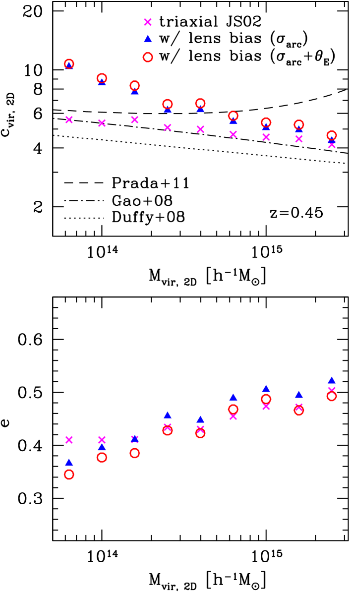
Figure 16 shows the mass-concentration relation derived from the projected mass distribution assuming a spherical mass distribution, which is relevant for the comparison with our lensing measurement, based on the semi-analytic calculation described above. We find that the enhancement of the concentration parameter due to the lensing bias is a strong function of the mass. For instance, when both the arc cross section and the Einstein radius are used for computing the lensing bias, the concentration parameter is enhanced by $\sim$80% for $M_{\rm vir}\sim 8\times 10^{13}h^{-1}M_{\odot}$, $\sim$30% for $M_{\rm vir}\sim 4\times 10^{14}h^{-1}M_{\odot}$, and $\sim$20% for $M_{\rm vir}\sim 10^{15}h^{-1}M_{\odot}$.

We also compare our result based on the triaxial model with other work studying the mass-concentration relation in $N$-body simulations based on the spherical NFW profile. We find that our mass-concentration relation has larger concentration than predicted by the relation of Duffy et al. (2008), which has been adopted for comparisons with lensing measurements in Oguri et al. (2009). On the other hand, Prada et al. (2011) concluded that concentrations of massive haloes evolve little with the redshift. As a result, concentrations predicted by the model of Prada et al. (2011) are much larger compared with the Duffy et al. (2008) relation predicts. We note that such little evolution of massive haloes have been noted by Zhao et al. (2003) and Zhao et al. (2009). Our mass-concentration relation based on the triaxial model resides in between the Duffy et al. (2008) and Prada et al. (2011) relations, and more resemble the relation presented by Gao et al. (2008) which was essentially the modification of the model proposed by Navarro et al. (1997).

Figure 17: The average concentration (filled squares) and ellipticity (open triangles) of the projected mass distributions as a function of the Einstein radius $\theta_{\rm E}$. They are derived from a triaxial halo model of Jing & Suto (2002) and include the effect of the lensing bias from the arc cross section.

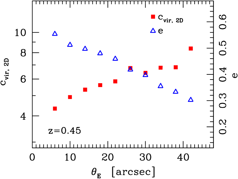
We also investigate the impact of the lensing bias on the ellipticity of the projected mass distribution. We find that the lensing bias due to the arc cross section tends to increase the mean ellipticity, which is understood by the fact that the ellipticity of the projected mass distribution significantly enhances the giant arc cross section (e.g., Meneghetti, Bartelmann, & Moscardini, 2003; Meneghetti et al., 2007). In contrast, the lensing bias due to the Einstein radius decreases the mean Einstein radius, because of the alignment of the major axis with the line-of-sight direction (Oguri & Blandford, 2009). Therefore, these two lensing biases counteract with each other. In either case, however, the effect of the lensing bias appears to be small, with the change of the mean ellipticity by $\sim 0.05$ at most.

Oguri & Blandford (2009) has shown that extreme lensing clusters having very large Einstein radii are more severely affected by the lensing bias. Thus we check the dependence of the concentration and projected ellipticity on the Einstein radius $\theta_{\rm E}$. For the mass distribution of the cluster, we assume a flat prior of $\log M_{\rm vir}$ between $10^{14}h^{-1}M_{\odot}$ and $10^{15}h^{-1}M_{\odot}$, and the number distribution predicted by the mass function of dark haloes above $10^{15}h^{-1}M_{\odot}$, which is expected to more or less resemble the selection function of our cluster sample. The result shown in Figure 17 indicate that both the concentration and ellipticity depend strongly on the Einstein radius such that clusters with larger Einstein radii are more concentrated and spherical. Again, this can be interpreted by the alignment of the major axis with the line-of-sight direction (Oguri & Blandford, 2009).

Appendix B Lensing analysis for individual clusters

We show for each cluster the critical curve of the best-fit strong lens modelling plotted on the Subaru/Suprime-cam $gri$-composite image ($2^{\prime}\times 2^{\prime}$; squares are positions of multiple images used for mass modelling), weak lensing mass map plotted on the Subaru/Suprime-cam $r$-band image (contours are drawn with spacing of $1\sigma$ noise level, and the cross indicates the position of the brightest cluster galaxy), and the tangential shear profile as well as the best-fit NFW profiles. The shading in the tangential profile plot indicates the measured Einstein radius and its $1\sigma$ error at the arc redshift.

Figure 18: SDSSJ0851+3331, SDSSJ0915+3826, SDSSJ0957+0509, SDSSJ1004+4112

Figure 19: SDSSJ1029+2623, SDSSJ1038+4849, SDSSJ1050+0017, RCS2J1055+5548

Figure 20: SDSSJ1110+6459, SDSSJ1115+5319, SDSSJ1138+2754, SDSSJ1152+3313

Figure 21: SDSSJ1152+0930, SDSSJ1209+2640, SDSSJ1226+2149, SDSSJ1226+2152

Figure 22: A1703, SDSSJ1315+5439, GHO132029+3155, SDSSJ1329+2243

Figure 23: SDSSJ1343+4155, SDSSJ1420+3955, SDSSJ1446+3032, SDSSJ1456+5702

Figure 24: SDSSJ1531+3414, SDSSJ1621+0607, SDSSJ1632+3500, SDSSJ2111-0114

References

- Baba et al. (2002) Baba H., et al., 2002, ASPC, 281, 298
- Bartelmann & Schneider (2001) Bartelmann M., Schneider P., 2001, PhR, 340, 291
- Bayliss (2011) Bayliss M. B., ApJ, in press (arXiv:1108.1175)
- Bayliss et al. (2010) Bayliss M. B., Wuyts E., Sharon K., Gladders M. D., Hennawi J. F., Koester B. P., Dahle H., 2010, ApJ, 720, 1559
- Bayliss et al. (2011a) Bayliss M. B., Gladders M. D., Oguri M., Hennawi J. F., Sharon K., Koester B. P., Dahle H., 2011a, ApJ, 727, L26
- Bayliss et al. (2011b) Bayliss M. B., Hennawi J. F., Gladders M. D., Koester B. P., Sharon K., Dahle H., Oguri M., 2011b, ApJS, 193, 8
- Becker & Kravtsov (2011) Becker M. R., Kravtsov A. V., 2011, ApJ, 740, 25
- Belokurov et al. (2009) Belokurov V., Evans N. W., Hewett P. C., Moiseev A., McMahon R. G., Sanchez S. F., King L. J., 2009, MNRAS, 392, 104
- Bertin (2006) Bertin E., 2006, ASPC, 351, 112
- Bertin (2009) Bertin E., 2009, MmSAI, 80, 422
- Bertin & Arnouts (1996) Bertin E., Arnouts S., 1996, A&AS, 117, 393
- Bett (2011) Bett P. E., 2011, arXiv:1108.3717
- Biviano (2008) Biviano A., 2008, arXiv:0811.3535
- Biviano & Poggianti (2009) Biviano A., Poggianti B. M., 2009, A&A, 501, 419
- Bradač et al. (2008) Bradač M., Allen S. W., Treu T., Ebeling H., Massey R., Morris R. G., von der Linden A., Applegate D., 2008, ApJ, 687, 959
- Broadhurst & Barkana (2008) Broadhurst T. J., Barkana R., 2008, MNRAS, 390, 1647
- Broadhurst et al. (2005) Broadhurst T., Takada M., Umetsu K., Kong X., Arimoto N., Chiba M., Futamase T., 2005, ApJ, 619, L143
- Broadhurst et al. (2008) Broadhurst T., Umetsu K., Medezinski E., Oguri M., Rephaeli Y., 2008, ApJ, 685, L9
- Bullock et al. (2001) Bullock J. S., Kolatt T. S., Sigad Y., Somerville R. S., Kravtsov A. V., Klypin A. A., Primack J. R., Dekel A., 2001, MNRAS, 321, 559
- Buote et al. (2007) Buote D. A., Gastaldello F., Humphrey P. J., Zappacosta L., Bullock J. S., Brighenti F., Mathews W. G., 2007, ApJ, 664, 123
- Clowe, De Lucia, & King (2004) Clowe D., De Lucia G., King L., 2004, MNRAS, 350, 1038
- Clowe et al. (2006) Clowe D., Bradač M., Gonzalez A. H., Markevitch M., Randall S. W., Jones C., Zaritsky D., 2006, ApJ, 648, L109
- Coe et al. (2010) Coe D., Benítez N., Broadhurst T., Moustakas L. A., 2010, ApJ, 723, 1678
- Corless & King (2007) Corless V. L., King L. J., 2007, MNRAS, 380, 149
- Corless et al. (2009) Corless V. L., King L. J., Clowe D., 2009, MNRAS, 393, 1235
- Comerford & Natarajan (2007) Comerford J. M., Natarajan P., 2007, MNRAS, 379, 190
- D’Aloisio & Natarajan (2011) D’Aloisio A., Natarajan P., 2011, MNRAS, 411, 1628
- Diehl et al. (2009) Diehl H. T., et al., 2009, ApJ, 707, 686
- Dodelson (2004) Dodelson S., 2004, PhRvD, 70, 023008
- Duffy et al. (2008) Duffy A. R., Schaye J., Kay S. T., Dalla Vecchia C., 2008, MNRAS, 390, L64
- Duffy et al. (2010) Duffy A. R., et al., 2010, MNRAS, 405, 2161
- Erben et al. (2001) Erben T., Van Waerbeke L., Bertin E., Mellier Y., Schneider P., 2001, A&A, 366, 717
- Ettori et al. (2010) Ettori S., Gastaldello F., Leccardi A., Molendi S., Rossetti M., Buote D., Meneghetti M., 2010, A&A, 524, A68
- Evans & Bridle (2009) Evans A. K. D., Bridle S., 2009, ApJ, 695, 1446
- Gao et al. (2008) Gao L., Navarro J. F., Cole S., Frenk C. S., White S. D. M., Springel V., Jenkins A., Neto A. F., 2008, MNRAS, 387, 536
- Gavazzi (2005) Gavazzi R., 2005, A&A, 443, 793
- Gralla et al. (2011) Gralla M. B., et al., 2011, ApJ, 737, 74
- Gruen et al. (2011) Gruen D., Bernstein G. M., Lam T. Y., Seitz S., 2011, MNRAS, 416, 1392
- Hamana et al. (2003) Hamana T., et al., 2003, ApJ, 597, 98
- Hamana et al. (2009) Hamana T., Miyazaki S., Kashikawa N., Ellis R. S., Massey R. J., Refregier A., Taylor J. E., 2009, PASJ, 61, 833
- Hansen et al. (2005) Hansen S. M., McKay T. A., Wechsler R. H., Annis J., Sheldon E. S., Kimball A., 2005, ApJ, 633, 122
- Hennawi et al. (2007) Hennawi J. F., Dalal N., Bode P., Ostriker J. P., 2007, ApJ, 654, 714
- Hennawi et al. (2008) Hennawi J. F., et al., 2008, AJ, 135, 664
- Heymans et al. (2006) Heymans C., et al., 2006, MNRAS, 368, 1323
- Hoekstra (2003) Hoekstra H., 2003, MNRAS, 339, 1155
- Hoekstra et al. (2004) Hoekstra H., Yee H. K. C., Gladders M. D., 2004, ApJ, 606, 67
- Hoekstra et al. (2011) Hoekstra H., Hartlap J., Hilbert S., van Uitert E., 2011, MNRAS, 412, 2095
- Hook et al. (2004) Hook I. M., Jørgensen I., Allington-Smith J. R., Davies R. L., Metcalfe N., Murowinski R. G., Crampton D., 2004, PASP, 116, 425
- Ilbert et al. (2009) Ilbert O., et al., 2009, ApJ, 690, 1236
- Inada et al. (2003) Inada N., et al., 2003, Natur, 426, 810
- Inada et al. (2006) Inada N., et al., 2006, ApJ, 653, L97
- Inada et al. (2008) Inada N., et al., 2008, AJ, 135, 496
- Inada et al. (2010) Inada N., et al., 2010, AJ, 140, 403
- Jee et al. (2007) Jee M. J., et al., 2007, ApJ, 661, 728
- Jing & Suto (2002) Jing Y. P., Suto Y., 2002, ApJ, 574, 538
- Johnston et al. (2007) Johnston D. E., et al., 2007, preprint (arXiv:0709.1159)
- Jullo et al. (2007) Jullo E., Kneib J.-P., Limousin M., Elíasdóttir Á., Marshall P. J., Verdugo T., 2007, NJPh, 9, 447
- Kaiser & Squires (1993) Kaiser N., Squires G., 1993, ApJ, 404, 441
- Kaiser et al. (1995) Kaiser N., Squires G., Broadhurst T., 1995, ApJ, 449, 460
- Katgert et al. (2004) Katgert P., Biviano A., Mazure A., 2004, ApJ, 600, 657
- Kazantzidis et al. (2004) Kazantzidis S., Kravtsov A. V., Zentner A. R., Allgood B., Nagai D., Moore B., 2004, ApJ, 611, L73
- Kneib & Natarajan (2011) Kneib J. P., Natarajan, P., 2011, in preparation
- Kochanek (2006) Kochanek C. S., 2006, glsw.conf, 91
- Koester et al. (2007) Koester B. P., et al., 2007, ApJ, 660, 221
- Koester et al. (2010) Koester B. P., Gladders M. D., Hennawi J. F., Sharon K., Wuyts E., Rigby J. R., Bayliss M. B., Dahle H., 2010, ApJ, 723, L73
- Komatsu et al. (2011) Komatsu E., et al., 2011, ApJS, 192, 18
- Kubo et al. (2009) Kubo J. M., Allam S. S., Annis J., Buckley-Geer E. J., Diehl H. T., Kubik D., Lin H., Tucker D., 2009, ApJ, 696, L61
- Kubo et al. (2010) Kubo J. M., et al., 2010, ApJ, 724, L137
- Lau et al. (2011) Lau E. T., Nagai D., Kravtsov A. V., Zentner A. R., 2011, ApJ, 734, 93
- Leauthaud et al. (2010) Leauthaud A., et al., 2010, ApJ, 709, 97
- Limousin et al. (2008) Limousin M., et al., 2008, A&A, 489, 23
- Lin, Mohr, & Stanford (2004) Lin Y.-T., Mohr J. J., Stanford S. A., 2004, ApJ, 610, 745
- Lin & Mohr (2007) Lin Y.-T., Mohr J. J., 2007, ApJS, 170, 71
- Mahdavi et al. (2007) Mahdavi A., Hoekstra H., Babul A., Balam D. D., Capak P. L., 2007, ApJ, 668, 806
- Mandelbaum et al. (2006a) Mandelbaum R., Hirata C. M., Broderick T., Seljak U., Brinkmann J., 2006a, MNRAS, 370, 1008
- Mandelbaum et al. (2006b) Mandelbaum R., Seljak U., Cool R. J., Blanton M., Hirata C. M., Brinkmann J., 2006b, MNRAS, 372, 758
- Mandelbaum, Seljak, & Hirata (2008) Mandelbaum R., Seljak U., Hirata C. M., 2008, JCAP, 8, 6
- Massey et al. (2007) Massey R., et al., 2007, MNRAS, 376, 13
- McCarthy et al. (2010) McCarthy I. G., et al., 2010, MNRAS, 406, 822
- Mead et al. (2010) Mead J. M. G., King L. J., Sijacki D., Leonard A., Puchwein E., McCarthy I. G., 2010, MNRAS, 406, 434
- Medezinski et al. (2007) Medezinski E., et al., 2007, ApJ, 663, 717
- Medezinski et al. (2010) Medezinski E., Broadhurst T., Umetsu K., Oguri M., Rephaeli Y., Benítez N., 2010, MNRAS, 405, 257
- Meneghetti, Bartelmann, & Moscardini (2003) Meneghetti M., Bartelmann M., Moscardini L., 2003, MNRAS, 340, 105
- Meneghetti et al. (2007) Meneghetti M., Argazzi R., Pace F., Moscardini L., Dolag K., Bartelmann M., Li G., Oguri M., 2007, A&A, 461, 25
- Meneghetti et al. (2010) Meneghetti M., Fedeli C., Pace F., Gottlöber S., Yepes G., 2010, A&A, 519, A90
- Merten et al. (2011) Merten J., et al., 2011, MNRAS, 417, 333
- Miyazaki et al. (2002) Miyazaki S., et al., 2002, PASJ, 54, 833
- Miyazaki et al. (2007) Miyazaki S., Hamana T., Ellis R. S., Kashikawa N., Massey R. J., Taylor J., Refregier A., 2007, ApJ, 669, 714
- Morandi, Pedersen, & Limousin (2011) Morandi A., Pedersen K., Limousin M., 2011, ApJ, 729, 37
- Morandi et al. (2011) Morandi A., Limousin M., Rephaeli Y., Umetsu K., Barkana R., Broadhurst T., Dahle H., 2011, MNRAS, 416, 2567
- Nagai & Kravtsov (2005) Nagai D., Kravtsov A. V., 2005, ApJ, 618, 557
- Natarajan & Refregier (2000) Natarajan P., Refregier A., 2000, ApJ, 538, L113
- Navarro et al. (1996) Navarro J. F., Frenk C. S., White S. D. M., 1996, ApJ, 462, 563
- Navarro et al. (1997) Navarro J. F., Frenk C. S., White S. D. M., 1997, ApJ, 490, 493
- Newman et al. (2009) Newman A. B., Treu T., Ellis R. S., Sand D. J., Richard J., Marshall P. J., Capak P., Miyazaki S., 2009, ApJ, 706, 1078
- Niederste-Ostholt et al. (2010) Niederste-Ostholt M., Strauss M. A., Dong F., Koester B. P., McKay T. A., 2010, MNRAS, 405, 2023
- Ofek, Seitz, & Klein (2008) Ofek E. O., Seitz S., Klein F., 2008, MNRAS, 389, 311
- Oguri (2010) Oguri M., 2010, PASJ, 62, 1017
- Oguri & Blandford (2009) Oguri M., Blandford R. D., 2009, MNRAS, 392, 930
- Oguri & Hamana (2011) Oguri M., Hamana T., 2011, MNRAS, 414, 1851
- Oguri & Keeton (2004) Oguri M., Keeton C. R., 2004, ApJ, 610, 663
- Oguri et al. (2003) Oguri M., Lee J., Suto Y., 2003, ApJ, 599, 7
- Oguri & Takada (2011) Oguri M., Takada M., 2011, PhRvD, 83, 023008
- Oguri et al. (2010) Oguri M., Takada M., Okabe N., Smith G. P., 2010, MNRAS, 405, 2215
- Oguri et al. (2005) Oguri M., Takada M., Umetsu K., Broadhurst T., 2005, ApJ, 632, 841
- Oguri et al. (2006) Oguri M., et al., 2006, AJ, 132, 999
- Oguri et al. (2008a) Oguri M., et al., 2008a, AJ, 135, 512
- Oguri et al. (2008b) Oguri M., et al., 2008b, ApJ, 676, L1
- Oguri et al. (2009) Oguri M., et al., 2009, ApJ, 699, 1038
- Okabe et al. (2010) Okabe N., Takada M., Umetsu K., Futamase T., Smith G. P., 2010, PASJ, 62, 811
- Okabe, Okura, & Futamase (2010) Okabe N., Okura Y., Futamase T., 2010, ApJ, 713, 291
- Ouchi et al. (2004) Ouchi M., et al., 2004, ApJ, 611, 685
- Parker et al. (2007) Parker L. C., Hoekstra H., Hudson M. J., van Waerbeke L., Mellier Y., 2007, ApJ, 669, 21
- Paz et al. (2006) Paz D. J., Lambas D. G., Padilla N., Merchán M., 2006, MNRAS, 366, 1503
- Postman et al. (2011) Postman M., et al., 2011, submitted to ApJS (arXiv:1106.3328)
- Prada et al. (2011) Prada F., Klypin A. A., Cuesta A. J., Betancort-Rijo J. E., Primack J., 2011, arXiv:1104.5130
- Richard et al. (2009) Richard J., Pei L., Limousin M., Jullo E., Kneib J. P., 2009, A&A, 498, 37
- Richard et al. (2010) Richard J., et al., 2010, MNRAS, 404, 325
- Rozo et al. (2009) Rozo E., et al., 2009, ApJ, 703, 601
- Rozo et al. (2011) Rozo E., Rykoff E., Koester B., Nord B., Wu H.-Y., Evrard A., Wechsler R., 2011, 740, 53
- Rudd, Zentner, & Kravtsov (2008) Rudd D. H., Zentner A. R., Kravtsov A. V., 2008, ApJ, 672, 19
- Rykoff et al. (2011) Rykoff E. S., et al., 2011, arXiv:1104.2089
- Sand et al. (2008) Sand D. J., Treu T., Ellis R. S., Smith G. P., Kneib J.-P., 2008, ApJ, 674, 711
- Schlegel, Finkbeiner, & Davis (1998) Schlegel D. J., Finkbeiner D. P., Davis M., 1998, ApJ, 500, 525
- Schmidt & Allen (2007) Schmidt R. W., Allen S. W., 2007, MNRAS, 379, 209
- Schrabback et al. (2010) Schrabback T., et al., 2010, A&A, 516, A63
- Sereno & Umetsu (2011) Sereno M., Umetsu K., 2011, MNRAS, 416, 3187
- Sereno, Jetzer, & Lubini (2010) Sereno M., Jetzer P., Lubini M., 2010, MNRAS, 403, 2077
- Sharon et al. (2005) Sharon K., et al., 2005, ApJ, 629, L73
- Umetsu & Broadhurst (2008) Umetsu K., Broadhurst T., 2008, ApJ, 684, 177
- Umetsu et al. (2010) Umetsu K., Medezinski E., Broadhurst T., Zitrin A., Okabe N., Hsieh B.-C., Molnar S. M., 2010, ApJ, 714, 1470
- Umetsu et al. (2011a) Umetsu K., Broadhurst T., Zitrin A., Medezinski E., Hsu L.-Y., 2011a, ApJ, 729, 127
- Umetsu et al. (2011b) Umetsu K., Broadhurst T., Zitrin A., Medezinski E., Coe D., Postman M., 2011b, ApJ, 738, 41
- Wen et al. (2011) Wen Z.-L., Han J.-L., Jiang Y.-Y., 2011, Research in Astronomy and Astrophysics, 11, 1185
- Yagi et al. (2002) Yagi M., Kashikawa N., Sekiguchi M., Doi M., Yasuda N., Shimasaku K., Okamura S., 2002, AJ, 123, 66
- York et al. (2000) York D. G., et al., 2000, AJ, 120, 1579
- Zhao et al. (2003) Zhao D. H., Jing Y. P., Mo H. J., Börner G., 2003, ApJ, 597, L9
- Zhao et al. (2009) Zhao D. H., Jing Y. P., Mo H. J., Börner G., 2009, ApJ, 707, 354
- Zitrin et al. (2010) Zitrin A., et al., 2010, MNRAS, 408, 1916
- Zitrin et al. (2011a) Zitrin A., Broadhurst T., Barkana R., Rephaeli Y., Benítez N., 2011a, MNRAS, 410, 1939
- Zitrin et al. (2011b) Zitrin A., et al., 2011b, arXiv:1103.5618
- Zitrin et al. (2011c) Zitrin A., Broadhurst T., Bartelmann M., Rephaeli Y., Oguri M., Benítez N., Hao J., Umetsu K., 2011c, arXiv:1105.2295