Collisions of Jets of Particles from Active Galactic Nuclei with Neutralino Dark Matter

Jinrui Huang, Arvind Rajaraman, and Tim M.P. Tait
Department of Physics and Astronomy,
University of California, Irvine, California 92697
Abstract

We examine the possibility that energetic Standard Model particles contained in the jets produced by active galactic nuclei (AGN) may scatter off of the dark matter halo which is expected to surround the AGN. In particular, if there are nearby states in the dark sector which can appear resonantly in the scattering, the cross section can be enhanced and a distinctive edge feature in the energy spectrum may appear. We examine bounds on supersymmetric models which may be obtained from the Fermi Gamma-ray Space Telescope observation of the nearby AGN Centaurus A.

1 Introduction

Active galactic nuclei (AGN) [1, 2, 3, 4, 5, 6, 7] are among the most powerful natural accelerators in the Universe, producing jets of charged particles which travel macroscopic distances and can even be imaged from the Earth through the subsequent production of high energy photons. While the nature of the jet constituents (proton or electron) remains a subject of some controversy, there is no doubt that they are among the highest energy and most interesting objects in the cosmos, with energies reaching into tens of GeV and with huge luminosities.

The supermassive black holes which power these jets are typically hosted in very large galaxies, where one would expect the largest concentrations of dark matter (DM) also occur. Taken together, the combination of dense dark matter with high energy particles represent a new opportunity to study the interactions of dark matter and Standard Model (SM) particles at high energies. Indeed, while particle accelerators on the Earth reach higher energies and with (much) better understood beams, the huge density of dark matter expected close to AGNs implies that they represent a unique opportunity to learn about dark matter interactions with high energy SM particles.

If there is some other particle in the “dark sector” which can be produced as a resonance in the scattering of dark matter with a jet particle, the rate for scattering in the high energy tail of the jet may be enhanced. Beam particles with energies E𝐸E greater than,

E𝐸\displaystyle E \displaystyle\geq 12me~2mχ~2mχ~12superscriptsubscript𝑚~𝑒2superscriptsubscript𝑚~𝜒2subscript𝑚~𝜒\displaystyle\frac{1}{2}\frac{m_{\tilde{e}}^{2}-m_{\tilde{\chi}}^{2}}{m_{\tilde{\chi}}} (1.1)

(where mχ~subscript𝑚~𝜒m_{\tilde{\chi}} is the mass of the dark matter and me~subscript𝑚~𝑒m_{\tilde{e}} the mass of the resonance) have sufficient energy to produce the resonance on-shell, leading to an enhancement of the cross section. Since the beam particles are presumably charged (so that they can be efficiently accelerated by the AGN), the resonant state should also be charged. As a result, its decays can produce gamma rays which can stick out from the background produced by the AGN and jet themselves. Such a situation is common in the most popular theories of dark matter, such as in supersymmetric theories in which a neutralino plays the role of dark matter [8], and which can be up-scattered by an energetic beam electron into a selectron 111Similarly, in theories with Universal Extra Dimensions [10], the dark matter particle may be a Kaluza-Klein excitation of the hypercharge vector boson [11, 12], which may up-scatter into a Kaluza-Klein mode of the electron [13]. and was first proposed by [9] and recently studied in [13]. Such a degeneracy may even be central to realizing a neutralino WIMP as dark matter, to allow for efficient enough coannihilation to produce the observed density from thermal freeze-out. In fact, a very degenerate selectron is challenging to detect at the LHC, because its visible decay products have energies controlled by me~mχ~subscript𝑚~𝑒subscript𝑚~𝜒m_{\tilde{e}}-m_{\tilde{\chi}}, and are typically very soft. Thus, the signal from AGNs is enhanced precisely where the LHC has difficulty, and can help study motivated but otherwise experimentally difficult regions of parameter space [14].

Since the resonant state must be charged, its subsequent de-excitation includes higher order processes in which a photon is produced in addition to the primary SM and dark matter decay products. While suppressed by α𝛼\alpha, such processes may be enhanced by collinear logarithms that rise when the photon is emitted along the same direction as the final state charged SM particle. Unlike charged particles, these radiated photons have very long mean free paths, and could be detected by detectors on the Earth as an indicator that the jet-DM scatterings are taking place. For dark matter masses on the order of a few hundred GeV, these photons fall precisely in the range for which the Fermi Gamma-ray Space Telescope [15] is sensitive, and thus it is precisely the right time to explore such signals. In fact, as pointed out in Ref. [13], the rise in cross section as beam particles cross the e~~𝑒\tilde{e} threshold leads to a very interesting feature in the spectrum of gamma rays, a rise in the number of high energy photons followed by a sharp edge. This feature provides an interesting discriminant from the background of gamma rays emitted from the jet itself, one which conventional astrophysical sources are expected to have difficulty faking. Inspired by Ref. [13], we study the dark matter and AGN electron jet scattering process in SUSY models, presenting the complete scattering amplitudes and performing an explicit check of gauge invariance. We scan the parameter space of neutralino and selectron masses to define precise constraints from the Fermi-LAT data.

This article is organized as follows. In Section 2, we discuss the astrophysical inputs to the computation, namely the density profile of dark matter around the AGN and the intensity and energy spectrum of the beam particles. In Section 3, we revisit the computation of the cross sections for scattering in supersymmetric theories. In Section 4 we examine the bounds one can place for different astrophysical assumptions. We conclude in Section 5.

2 Astrophysical Inputs

In this section, we discuss the astrophysical inputs to our estimates. These boil down into the properties of particles inside the AGN jet, and the density of dark matter surrounding it. In both cases, we follow closely the discussion of Ref. [13], which contains a more detailed discussion, and study of the impact varying these parameters has on the signal. We restrict ourselves to looking at Centaurus A, which offers a good balance of being relatively close by (D3.7similar-to𝐷3.7D\sim 3.7 Mpc [16]) as well as a massive object surrounded by a dense halo of dark matter.

2.1 Dark Matter Distribution

The impact of the dark matter distribution is through its integral along the “line of sight” of the jet particles,

δDMsubscript𝛿DM\displaystyle\delta_{\rm DM} \displaystyle\equiv rminrmax𝑑rρ(r)subscriptsuperscriptsubscript𝑟maxsubscript𝑟mindifferential-d𝑟𝜌𝑟\displaystyle\int^{r_{\rm max}}_{r_{\rm min}}dr~{}\rho(r) (2.1)

where ρ(r)𝜌𝑟\rho(r) is the density of dark matter at a radial distance r𝑟r from the center of the AGN, rminsubscript𝑟minr_{\rm min} characterizes the minimum distance of interest (the base of the jet), and rmaxsubscript𝑟maxr_{\rm max} the distance at which the jet loses cohesion and becomes irrelevant. In practice, results depend sensitively on rminsubscript𝑟minr_{\rm min} and are rather insensitive to rmaxsubscript𝑟maxr_{\rm max} [13] due to the fact that dark matter density distribution ρ(r)𝜌𝑟\rho(r) drops steeply as the the radius r increases.

The dark matter density distribution surrounding a compact object was modeled in Ref. [17] in the collisionless limit and under the assumption that the central black hole grew adiabatically by accretion. The resulting steady-state distribution is characterized by a central spike of dark matter, which gets depleted in the core by pair annihilation. The resulting distribution is thus sensitive to the underlying particle physics model of dark matter, with the central density enhanced for WIMPs with very low (or in the case of a purely asymmetric dark matter halo, zero) annihilation cross sections. Ref [17] begins with a cusped density profile ρi(r)=ρ0(r/r0)γsubscript𝜌i𝑟subscript𝜌0superscript𝑟subscript𝑟0𝛾\rho_{\rm i}(r)=\rho_{0}(r/r_{0})^{-\gamma}, and determines a final profile (close to the center) of the form,

ρ(r)𝜌𝑟\displaystyle\rho(r) =\displaystyle= ρ(r)ρcoreρ(r)+ρcore,superscript𝜌𝑟subscript𝜌coresuperscript𝜌𝑟subscript𝜌core\displaystyle\frac{\rho^{\prime}(r)~{}\rho_{\rm core}}{\rho^{\prime}(r)+\rho_{\rm core}}~{}, (2.2)

where the core density is given in terms of the velocity-averaged annihilation rate σvdelimited-⟨⟩𝜎𝑣\langle\sigma v\rangle and the age of the black hole tBHsubscript𝑡BHt_{\rm BH} as,

ρcoresubscript𝜌core\displaystyle\rho_{\rm core} similar-to-or-equals\displaystyle\simeq mχ~σvtBH.subscript𝑚~𝜒delimited-⟨⟩𝜎𝑣subscript𝑡BH\displaystyle\frac{m_{\tilde{\chi}}}{\langle\sigma v\rangle~{}t_{\rm BH}}~{}. (2.3)

The dependence on r𝑟r is contained in the function,

ρ(r)superscript𝜌𝑟\displaystyle\rho^{\prime}(r) =\displaystyle= ρ0(Rspr0)γ(14RSr)3(Rspr)γsp,subscript𝜌0superscriptsubscript𝑅spsubscript𝑟0𝛾superscript14subscript𝑅𝑆𝑟3superscriptsubscript𝑅sp𝑟subscript𝛾sp\displaystyle\rho_{0}\left(\frac{R_{\rm sp}}{r_{0}}\right)^{-\gamma}\left(1-\frac{4R_{S}}{r}\right)^{3}\left(\frac{R_{\rm sp}}{r}\right)^{\gamma_{\rm sp}}~{}, (2.4)

where γspsubscript𝛾sp\gamma_{\rm sp} is slope of the density profile in the dark matter spike, Rspsubscript𝑅spR_{\rm sp} its radius, and RSsubscript𝑅𝑆R_{S} is the Schwarzschild radius. Below 4RS4subscript𝑅𝑆4R_{S}, the dark matter is accreted into the black hole, and has ρ=0𝜌0\rho=0. The spike radius and power are given by,

Rsp=αγr0(MBHρ0r03)13γsubscript𝑅spsubscript𝛼𝛾subscript𝑟0superscriptsubscript𝑀BHsubscript𝜌0superscriptsubscript𝑟0313𝛾\displaystyle R_{\rm sp}=\alpha_{\gamma}~{}r_{0}~{}\left(\frac{M_{\rm BH}}{\rho_{0}~{}r_{0}^{3}}\right)^{\frac{1}{3-\gamma}} andand\displaystyle~{}~{}{\rm and}~{}~{} γsp=92γ4γ,subscript𝛾sp92𝛾4𝛾\displaystyle\gamma_{\rm sp}=\frac{9-2\gamma}{4-\gamma}~{}, (2.5)

where αγ0.293γ4/9similar-tosubscript𝛼𝛾0.293superscript𝛾49\alpha_{\gamma}\sim 0.293\gamma^{4/9} for γ1much-less-than𝛾1\gamma\ll 1  [17]. This analysis neglects the influence of stellar populations close to the the supermassive black hole, which can gravitationally scatter dark matter out of the spike, resulting in a somewhat shallower profile [18].

Following Ref. [13], we normalize the distribution such that it falls within the uncertainty on the measured mass of the black hole itself. The mass of the black hole is determined by measurements of stellar kinematics to be [19],

MBH=(5.5±3.0)×107Msubscript𝑀BHplus-or-minus5.53.0superscript107subscript𝑀direct-product\displaystyle M_{\rm BH}=(5.5\pm 3.0)\times 10^{7}M_{\odot} (2.6)

which corresponds to RS5×106pcsimilar-to-or-equalssubscript𝑅𝑆5superscript106pcR_{S}\simeq 5\times 10^{-6}~{}{\rm pc}. Given a choice of γ𝛾\gamma, we determine ρ0subscript𝜌0\rho_{0} by requiring,

3×10⁷M3superscript107subscript𝑀direct-product\displaystyle 3\times 10^{7}M_{\odot} \displaystyle\geq 4RS105RS𝑑r4πr2ρ(r),superscriptsubscript4subscript𝑅𝑆superscript105subscript𝑅𝑆differential-d𝑟4𝜋superscript𝑟2𝜌𝑟\displaystyle\int_{4R_{S}}^{10^{5}R_{S}}dr~{}4\pi r^{2}~{}\rho(r)~{}, (2.7)

where 105RSsuperscript105subscript𝑅𝑆10^{5}R_{S} characterizes the distances at which the stellar populations are measured.

Ultimately, the factor δDMsubscript𝛿DM\delta_{\rm DM} is very sensitive to the product σv×tBHdelimited-⟨⟩𝜎𝑣subscript𝑡BH\langle\sigma v\rangle\times t_{\rm BH}, which determines the density within the spike. For black hole ages between 108superscript10810^{8} to 1010superscript101010^{10} years and cross sections ranging from 1026superscript102610^{-26} cm3 s-1 (appropriate for a thermal relic) to 1030superscript103010^{-30} cm3 s-1 (typical for the “coannihilation” region of the MSSM, in which the superpartners of the charged leptons play an active role in freeze-out), one finds δDMsubscript𝛿DM\delta_{\rm DM} ranging from,

δDM108to1011M/pc3similar-tosubscript𝛿DMsuperscript108tosuperscript1011subscript𝑀direct-productsuperscriptpc3\displaystyle\delta_{\rm DM}\sim 10^{8}~{}~{}{\rm to}~{}~{}10^{11}~{}~{}{M_{\odot}}~{}/~{}{{\rm pc}^{3}} (2.8)

with rather mild dependence on the choices of γ𝛾\gamma, rminsubscript𝑟minr_{\rm min}, and r0rmax15similar-tosubscript𝑟0subscript𝑟maxsimilar-to15r_{0}\sim r_{\rm max}\sim 15 kpc [13].

2.2 AGN Jet Particles

For our purposes, the details of the AGN jet geometry are not very important, while modeling the energy distribution of particles in the jet is crucial. We assume most of the particles in the Centaurus A jet are electrons. Based on observation of emitted gamma rays by the Fermi LAT experiment [20], we assume the distribution in the electron boost is a broken power law,

dΦe(AGN)dγ(γ)=12keγs1[1+(γγbr)(s2s1)]1(γmin<γ<γmax).𝑑superscriptsubscriptΦ𝑒AGN𝑑superscript𝛾superscript𝛾12subscript𝑘𝑒superscript𝛾subscript𝑠1superscriptdelimited-[]1superscriptsuperscript𝛾subscriptsuperscript𝛾𝑏𝑟subscript𝑠2subscript𝑠11subscriptsuperscript𝛾minsuperscript𝛾subscriptsuperscript𝛾max\frac{d\Phi_{e}^{\rm(AGN)}}{d\gamma^{\prime}}(\gamma^{\prime})~{}=~{}\frac{1}{2}k_{e}\gamma^{\prime\,-s_{1}}\left[1+(\frac{\gamma^{\prime}}{\gamma^{\prime}_{br}})^{(s_{2}-s_{1})}\right]^{-1}~{}~{}~{}~{}~{}~{}~{}~{}~{}~{}~{}~{}~{}\left(\gamma^{\prime}_{\rm min}<\gamma^{\prime}<\gamma^{\prime}_{\rm max}\right)\;. (2.9)

Here the primed variables refer to the “blob frame”, in which the electrons move isotropically. The parameters s1subscript𝑠1s_{1}, s2subscript𝑠2s_{2}, γbrsubscriptsuperscript𝛾𝑏𝑟\gamma^{\prime}_{br}, γminsubscriptsuperscript𝛾min\gamma^{\prime}_{\rm min} and γmaxsubscriptsuperscript𝛾max\gamma^{\prime}_{\rm max} are fixed to [20]

s1=1.8,s2=3.5,γbr=4×10⁵,γmin=8×10²,γmax=108.formulae-sequencesubscript𝑠11.8formulae-sequencesubscript𝑠23.5formulae-sequencesuperscriptsubscript𝛾𝑏𝑟4superscript105formulae-sequencesuperscriptsubscript𝛾min8superscript102superscriptsubscript𝛾maxsuperscript108\displaystyle s_{1}=1.8,\qquad s_{2}=3.5,\qquad\gamma_{br}^{\prime}=4\times 10^{5},\qquad\gamma_{\rm min}^{\prime}=8\times 10^{2},\qquad\gamma_{\rm max}^{\prime}=10^{8}\;. (2.10)

The normalization kesubscript𝑘𝑒k_{e} can be determined from the jet power in electrons, which is defined in the black hole frame as,

Lesubscript𝐿𝑒\displaystyle L_{e} =\displaystyle= 11dμΓB(1βBμ)γminγmax𝑑γ(meγ)dΦeAGNdγ(γ(ΓB(1βBμ))),superscriptsubscript11𝑑𝜇subscriptΓ𝐵1subscript𝛽𝐵𝜇superscriptsubscriptsubscript𝛾minsubscript𝛾maxdifferential-d𝛾subscript𝑚𝑒𝛾𝑑superscriptsubscriptΦ𝑒𝐴𝐺𝑁𝑑𝛾𝛾subscriptΓ𝐵1subscript𝛽𝐵𝜇\displaystyle\int_{-1}^{1}~{}\frac{d\mu}{\Gamma_{B}(1-\beta_{B}\mu)}~{}\int_{\gamma_{\rm min}}^{\gamma_{\rm max}}~{}d\gamma(m_{e}\gamma)~{}~{}\frac{d\Phi_{e}^{AGN}}{d\gamma}\biggl{(}\gamma(\Gamma_{B}(1-\beta_{B}\mu))\biggr{)}\;, (2.11)

where μ=cosθ𝜇𝜃\mu=\cos\theta (θ𝜃\theta is the polar angle with respect to the jet axis) and γ=ϵ/me𝛾italic-ϵsubscript𝑚𝑒\gamma=\epsilon/m_{e} where ϵitalic-ϵ\epsilon is the energy of the electron. Similarly, the primed variables in the blob frame are μ=cosθsuperscript𝜇superscript𝜃\mu^{\prime}=\cos\theta^{\prime} and γ=ϵ/mesuperscript𝛾superscriptitalic-ϵsubscript𝑚𝑒\gamma^{\prime}=\epsilon^{\prime}/m_{e}. The quantities in the two frames are related by the blob velocity βBsubscript𝛽𝐵\beta_{B} and boost ΓB=1/1βB2subscriptΓ𝐵11superscriptsubscript𝛽𝐵2\Gamma_{B}=1/\sqrt{1-\beta_{B}^{2}} ( 3similar-toabsent3\sim 3 for Centaurus A) as,

μ=μβB1βBμ,γ=γΓB(1βBμ),formulae-sequencesuperscript𝜇𝜇subscript𝛽𝐵1subscript𝛽𝐵𝜇superscript𝛾𝛾subscriptΓ𝐵1subscript𝛽𝐵𝜇\displaystyle\mu^{\prime}=\frac{\mu-\beta_{B}}{1-\beta_{B}~{}\mu}\;,\qquad\gamma^{\prime}=\gamma~{}\Gamma_{B}~{}(1-\beta_{B}\mu)\;, (2.13)

or equivalently,

μ=μ+βB1+βBμ,γ=γΓB(1βBμ).formulae-sequence𝜇superscript𝜇subscript𝛽𝐵1subscript𝛽𝐵superscript𝜇𝛾superscript𝛾subscriptΓ𝐵1subscript𝛽𝐵𝜇\displaystyle\mu=\frac{\mu^{\prime}+\beta_{B}}{1+\beta_{B}\mu^{\prime}}\;,\qquad\gamma=\frac{\gamma^{\prime}}{\Gamma_{B}~{}(1-\beta_{B}\mu)}\;. (2.14)

The limits on the γ𝛾\gamma integral are given by,

γmin=γminΓB(1βBμ),γmax=γmaxΓB(1βBμ),formulae-sequencesubscript𝛾minsubscriptsuperscript𝛾minsubscriptΓ𝐵1subscript𝛽𝐵𝜇subscript𝛾maxsubscriptsuperscript𝛾maxsubscriptΓ𝐵1subscript𝛽𝐵𝜇\displaystyle\gamma_{\rm min}=\frac{\gamma^{\prime}_{\rm min}}{\Gamma_{B}~{}(1-\beta_{B}\mu)}\;,\qquad\gamma_{\rm max}=\frac{\gamma^{\prime}_{\rm max}}{\Gamma_{B}~{}(1-\beta_{B}\mu)}\;, (2.15)

whereas the limits on μ𝜇\mu in the black hole frame correspond to 0.910.910.9-1, leading to a highly collimated jet of electrons.

The function dΦe(AGN)/dγ𝑑superscriptsubscriptΦ𝑒AGN𝑑𝛾{d\Phi_{e}^{\rm(AGN)}}/{d\gamma} can be written explicitly as,

dΦedγ(AGN)(γ(ΓB(1βBμ)))=12ke[γΓB(1βBμ)]s1[1+(γ(ΓB(1βBμ))/γbr)s2s1]1.superscript𝑑subscriptΦ𝑒𝑑𝛾AGN𝛾subscriptΓ𝐵1subscript𝛽𝐵𝜇12subscript𝑘𝑒superscriptdelimited-[]𝛾subscriptΓ𝐵1subscript𝛽𝐵𝜇subscript𝑠1superscriptdelimited-[]1superscript𝛾subscriptΓ𝐵1subscript𝛽𝐵𝜇superscriptsubscript𝛾𝑏𝑟subscript𝑠2subscript𝑠11\frac{d\Phi_{e}}{d\gamma}^{\rm(AGN)}\biggl{(}\gamma(\Gamma_{B}(1-\beta_{B}\mu))\biggr{)}=\frac{1}{2}k_{e}\biggl{[}\gamma\Gamma_{B}(1-\beta_{B}\mu)\biggr{]}^{-s_{1}}\biggl{[}1+\biggl{(}\gamma(\Gamma_{B}(1-\beta_{B}\mu))/\gamma_{br}^{\prime}\biggr{)}^{s_{2}-s_{1}}\biggr{]}^{-1}\;. (2.16)

Saturating the upper limit of Le1046subscript𝐿𝑒superscript1046L_{e}\leq 10^{46} erg s1superscript𝑠1s^{-1} [13], we arrive at

12ke=4.2088×1049s1.12subscript𝑘𝑒4.2088superscript1049superscript𝑠1\displaystyle\frac{1}{2}k_{e}=4.2088\times 10^{49}s^{-1}~{}. (2.17)

3 Cross Sections

Refer to caption
(a)
Refer to caption
(b)
Refer to caption
(c)
Refer to caption
(d)
Refer to caption
(e)
Refer to caption
(f)
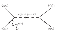
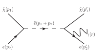
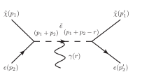
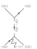
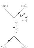
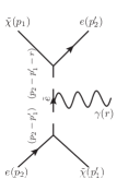
Figure 1: Feynman diagrams for the process eχ~eχ~γsuperscript𝑒~𝜒superscript𝑒~𝜒𝛾e^{-}~{}\tilde{\chi}\rightarrow e^{-}~{}\tilde{\chi}~{}\gamma through e~~𝑒\tilde{e} exchange. The amplitudes corresponding to these diagrams are, sequentially, M1M6subscript𝑀1subscript𝑀6M_{1}-M_{6}.

The total cross section for the process eχ~eχ~γ𝑒~𝜒𝑒~𝜒𝛾e~{}\tilde{\chi}\rightarrow e~{}\tilde{\chi}~{}\gamma may be written,

dσ=(2π)4δ4(p1+p2p1p2r)14mχ~E2d3p1(2π)32E1d3p2(2π)22E2d3r(2π)32Eγ||2,𝑑𝜎superscript2𝜋4superscript𝛿4subscript𝑝1subscript𝑝2superscriptsubscript𝑝1superscriptsubscript𝑝2𝑟14subscript𝑚~𝜒subscript𝐸2superscript𝑑3superscriptsubscript𝑝1superscript2𝜋32superscriptsubscript𝐸1superscript𝑑3superscriptsubscript𝑝2superscript2𝜋22superscriptsubscript𝐸2superscript𝑑3𝑟superscript2𝜋32subscript𝐸𝛾superscript2d\sigma=(2\pi)^{4}\delta^{4}(p_{1}+p_{2}-p_{1}^{\prime}-p_{2}^{\prime}-r)\frac{1}{4m_{\tilde{\chi}}E_{2}}\frac{d^{3}p_{1}^{\prime}}{(2\pi)^{3}2E_{1}^{\prime}}\frac{d^{3}p_{2}^{\prime}}{(2\pi)^{2}2E_{2}^{\prime}}\frac{d^{3}r}{(2\pi)^{3}2E_{\gamma}}\sum|\mathcal{M}|^{2}\;, (3.1)

where the ||2superscript2\sum|\mathcal{M}|^{2} is the sum of all of the matrix elements squared. In addition to the s𝑠s-channel contributions included in [13]), the u𝑢u-channel e~~𝑒\tilde{e} exchange diagrams are also included, as shown in the Fig. 1. We ignore t𝑡t-channel contributions mediated by the SM Z𝑍Z boson as it is non-resonant, and thus negligible. The amplitudes corresponding to these diagrams are labelled M1M6subscript𝑀1subscript𝑀6M_{1}-M_{6}.

The experimental observable is the distribution of photon energies, νSνEγ2dΦγdEγ𝜈subscript𝑆𝜈superscriptsubscript𝐸𝛾2𝑑subscriptΦ𝛾𝑑subscript𝐸𝛾\nu S_{\nu}\equiv E_{\gamma}^{2}\frac{d\Phi_{\gamma}}{dE_{\gamma}} at a fixed angle relative to the jet axis (68similar-toabsentsuperscript68\sim 68^{\circ} for the Centaurus A). For fixed incoming electron energy, we integrate over the phase space of the final state neutralino and electron, resulting in d2σ/dEγdΩγsuperscript𝑑2𝜎𝑑subscript𝐸𝛾𝑑subscriptΩ𝛾{d^{2}\sigma}/{dE_{\gamma}d\Omega_{\gamma}}. We work in the rest frame of the initial neutralino dark matter particle, which is expected to be moving non-relativistically (300similar-toabsent300\sim 300 km/s [21]) in the rest frame of the Earth. d2σ/dEγdΩγsuperscript𝑑2𝜎𝑑subscript𝐸𝛾𝑑subscriptΩ𝛾{d^{2}\sigma}/{dE_{\gamma}d\Omega_{\gamma}} can be expressed,

d2σdEγdΩγ=1(2π)214mχ~E218E1𝑑Ωp2(E2Eγ1|1+J|||2),superscript𝑑2𝜎𝑑subscript𝐸𝛾𝑑subscriptΩ𝛾1superscript2𝜋214subscript𝑚~𝜒subscript𝐸218superscriptsubscript𝐸1differential-dsubscriptΩsuperscriptsubscript𝑝2superscriptsubscript𝐸2subscript𝐸𝛾11𝐽superscript2\frac{d^{2}\sigma}{dE_{\gamma}d\Omega_{\gamma}}=\frac{1}{(2\pi)^{2}}\frac{1}{4m_{\tilde{\chi}}E_{2}}\frac{1}{8E_{1}^{\prime}}\int d\Omega_{p_{2}^{\prime}}\biggl{(}E_{2}^{\prime}E_{\gamma}\frac{1}{|1+J|}\sum|\mathcal{M}|^{2}\biggr{)}, (3.2)

where J𝐽J is a Jacobian factor from the integration of the function δ4(p1+p2p1p2r)superscript𝛿4subscript𝑝1subscript𝑝2superscriptsubscript𝑝1superscriptsubscript𝑝2𝑟\delta^{4}(p_{1}+p_{2}-p_{1}^{\prime}-p_{2}^{\prime}-r) over dE2𝑑superscriptsubscript𝐸2dE_{2}^{\prime} and can be explicitly written as

J𝐽\displaystyle J =\displaystyle= E2E1(p1+p2r)p2E1E2superscriptsubscript𝐸2superscriptsubscript𝐸1subscript𝑝1subscript𝑝2𝑟superscriptsubscript𝑝2superscriptsubscript𝐸1superscriptsubscript𝐸2\displaystyle\frac{E_{2}^{\prime}}{E_{1}^{\prime}}-\frac{(\vec{p}_{1}+\vec{p}_{2}-\vec{r})\cdot\vec{p}_{2}^{\prime}}{E_{1}^{\prime}E_{2}^{\prime}} (3.3)
=\displaystyle= E2E1(p2xrx)p2x+(p2yry)p2y+(p2zrz)p2zE1E2.superscriptsubscript𝐸2superscriptsubscript𝐸1subscript𝑝2𝑥subscript𝑟𝑥superscriptsubscript𝑝2𝑥subscript𝑝2𝑦subscript𝑟𝑦superscriptsubscript𝑝2𝑦subscript𝑝2𝑧subscript𝑟𝑧superscriptsubscript𝑝2𝑧superscriptsubscript𝐸1superscriptsubscript𝐸2\displaystyle\frac{E_{2}^{\prime}}{E_{1}^{\prime}}-\frac{(p_{2x}-r_{x})p_{2x}^{\prime}+(p_{2y}-r_{y})p_{2y}^{\prime}+(p_{2z}-r_{z})p_{2z}^{\prime}}{E_{1}^{\prime}E_{2}^{\prime}}. (3.4)

The full expression for the amplitude squared may be found in Appendix A. The cross section is enhanced in three kinematic configurations:

  • M13subscript𝑀13M_{1-3} are resonantly enhanced when the incoming electron energy is such that the intermediate selectron is approximately on-shell [9].

  • M2subscript𝑀2M_{2} and M5subscript𝑀5M_{5} have a collinear enhancement when the emitted photon lines up with the final state electron [13].

  • M2subscript𝑀2M_{2} and M5subscript𝑀5M_{5} have a soft enhancement for low energy photon emission.

Note that because the jet axis makes a fixed angle with respect to the line of sight from the Earth, there is no possibility of a collinear enhancement from the initial electron in M1subscript𝑀1M_{1} and M4subscript𝑀4M_{4}. In practice, the soft enhancement (the infinity of which is formally matched by the one-loop QED correction to eχ~eχ~superscript𝑒~𝜒superscript𝑒~𝜒e^{-}~{}\tilde{\chi}\rightarrow e^{-}~{}\tilde{\chi} scattering) is not observationally interesting. The dominant contribution comes from the on-shell selectron, collinear photon region of M2subscript𝑀2M_{2}:

|M2|2superscriptsubscript𝑀22\displaystyle|M_{2}|^{2} =\displaystyle= αeff(p1r)(p1p2)|Σs|2((p2r)me22),subscript𝛼effsuperscriptsubscript𝑝1𝑟subscript𝑝1subscript𝑝2superscriptsubscriptΣ𝑠2superscriptsubscript𝑝2𝑟superscriptsubscript𝑚𝑒22\displaystyle\frac{\alpha_{\mbox{\tiny{eff}}}~{}~{}(p_{1}^{\prime}\cdot r)(p_{1}\cdot p_{2})}{|\Sigma_{s}|^{2}~{}\biggl{(}(p_{2}^{\prime}\cdot r)-\frac{m_{e}^{2}}{2}\biggr{)}}\;, (3.5)

where αeff=4παEM(aL4+aR4)subscript𝛼eff4𝜋subscript𝛼EMsuperscriptsubscript𝑎L4superscriptsubscript𝑎R4\alpha_{\mbox{\tiny{eff}}}=4\pi\alpha_{\mbox{\tiny{EM}}}(a_{\mbox{\tiny{L}}}^{4}+a_{\mbox{\tiny{R}}}^{4}) is the effective neutralino-selectron-electron coupling. We assume the left- and right-handed selectrons are degenerate in mass, and a mostly bino neutralino, for which,

aR2superscriptsubscript𝑎R2\displaystyle a_{\mbox{\tiny{R}}}^{2} =\displaystyle= 2gw2tanθw2,2superscriptsubscript𝑔𝑤2superscriptsubscript𝜃𝑤2\displaystyle 2g_{w}^{2}\tan\theta_{w}^{2}~{}, (3.6)
aL2superscriptsubscript𝑎L2\displaystyle a_{\mbox{\tiny{L}}}^{2} =\displaystyle= aR2/4.superscriptsubscript𝑎R24\displaystyle a_{\mbox{\tiny{R}}}^{2}/4~{}. (3.7)

The factor 1/|Σs|21superscriptsubscriptΣ𝑠21/|\Sigma_{s}|^{2} is the selectron propagator, which has been modified to maintain gauge invariance222Proof of gauge invariance (correcting Ref [13]) can be found in Appendix B., using the prescription of Ref. [23]. To avoid the divergence from soft radiation, (p2r)superscriptsubscript𝑝2𝑟(p_{2}^{\prime}\cdot r) in the propagator has been shifted by me2/2superscriptsubscript𝑚𝑒22{m_{e}^{2}}/{2}.

Refer to caption
Refer to caption
Refer to caption
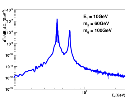
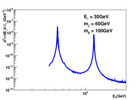
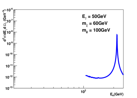
Figure 2: Differential cross sections, d2σ/dEγdΩγsuperscript𝑑2𝜎𝑑subscript𝐸𝛾𝑑subscriptΩ𝛾d^{2}\sigma/dE_{\gamma}d\Omega_{\gamma} for the process eχ~eχ~γsuperscript𝑒~𝜒superscript𝑒~𝜒𝛾e^{-}\tilde{\chi}\rightarrow e^{-}\tilde{\chi}\gamma, for a neutralino mass of 60 GeV and selectron mass of 100 GeV, and fixed photon energies (top to bottom) of 10 GeV, 30 GeV, and 50 GeV.

The differential cross sections d2σ/dEedΩγsuperscript𝑑2𝜎𝑑subscript𝐸𝑒𝑑subscriptΩ𝛾d^{2}\sigma/dE_{e}d\Omega_{\gamma} are shown as a function of the incoming electron energy in Fig. 2, for fixed photon energies of 10 GeV, 30 GeV and 50 GeV. As a benchmark point, we have chosen the mass of the neutralino to be mχ~=60subscript𝑚~𝜒60m_{\tilde{\chi}}=60 GeV and the mass of the selectron to be me~=100subscript𝑚~𝑒100m_{\tilde{e}}=100 GeV. Notice that for a photon energy of 10 GeV or 30 GeV, there are two peaks which arise from the (shifted) resonant behavior of M2subscript𝑀2M_{2} and M1subscript𝑀1M_{1} separately. However, as the photon energy increases, the incoming electron energy must be large enough to produce such a hard photon in the scattering process, closing off the possibility for scattering (for fixed Eγsubscript𝐸𝛾E_{\gamma}) below a certain threshold. Once the threshold rises above me~/2similar-toabsentsubscript𝑚~𝑒2\sim m_{\tilde{e}}/2, it becomes impossible to produce a final state photon from an on-shell e~~𝑒\tilde{e} decay, and the M2subscript𝑀2M_{2} resonance effectively disappears.

4 Bounds on Supersymmetric Parameter Space

Putting the astrophysical inputs together with the cross section, we have:

dΦγdEγ𝑑subscriptΦ𝛾𝑑subscript𝐸𝛾\displaystyle\frac{d\Phi_{\gamma}}{dE_{\gamma}} =\displaystyle= (δDM)×𝑑Ee(1D2dΦeAGNdEe)×(1mχ~d2σdEγdΩγ).subscript𝛿DMdifferential-dsubscript𝐸𝑒1superscript𝐷2𝑑superscriptsubscriptΦ𝑒AGN𝑑subscript𝐸𝑒1subscript𝑚~𝜒superscript𝑑2𝜎𝑑subscript𝐸𝛾𝑑subscriptΩ𝛾\displaystyle\biggl{(}\delta_{\rm DM}\biggr{)}\times\int~{}dE_{e}~{}\biggl{(}\frac{1}{D^{2}}\frac{d\Phi_{e}^{\mbox{\tiny{AGN}}}}{dE_{e}}\biggr{)}\times\biggl{(}\frac{1}{m_{\tilde{\chi}}}\frac{d^{2}\sigma}{dE_{\gamma}d\Omega_{\gamma}}\biggr{)}. (4.1)

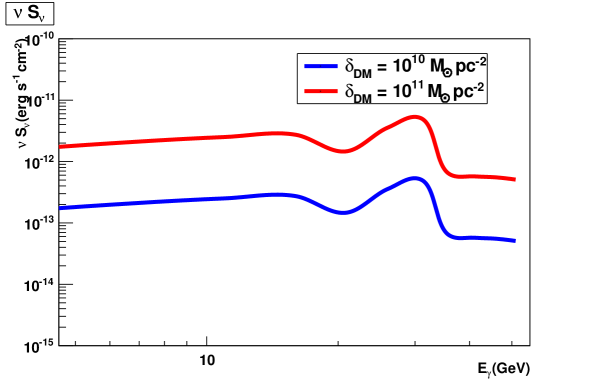
where the three factors δDMsubscript𝛿𝐷𝑀\delta_{DM}, dΦeAGN/dEe𝑑superscriptsubscriptΦ𝑒AGN𝑑subscript𝐸𝑒{d\Phi_{e}^{\mbox{\tiny{AGN}}}}/{dE_{e}} and d2σ/dEγdΩγsuperscript𝑑2𝜎𝑑subscript𝐸𝛾𝑑subscriptΩ𝛾{d^{2}\sigma}/{dE_{\gamma}d\Omega_{\gamma}} have been discussed in Sections 2.1, 2.2 and 3, respectively. We adopt two choices of δDM=1010Mpc2subscript𝛿DMsuperscript1010subscript𝑀direct-productsuperscriptpc2\delta_{\rm DM}=10^{10}~{}M_{\odot}~{}{\rm pc}^{-2} and δDM=1011Mpc2subscript𝛿DMsuperscript1011subscript𝑀direct-productsuperscriptpc2\delta_{\rm DM}=10^{11}~{}M_{\odot}~{}{\rm pc}^{-2} and to begin with, the benchmark point with a bino neutralino of mass mχ~=60subscript𝑚~𝜒60m_{\tilde{\chi}}=60 GeV and degenerate left- and right-handed sleptons of masses me~=100subscript𝑚~𝑒100m_{\tilde{e}}=100 GeV. In Figure 3, we plot the distribution of photon energies for the benchmark point, for both values of δDMsubscript𝛿DM\delta_{\rm DM} discussed above. We note the drop at energies around Eγ35similar-tosubscript𝐸𝛾35E_{\gamma}\sim 35 GeV, where, as discussed above, the required photon energy is so large that it is no longer produced efficiently from on-shell intermediate selectrons.
Refer to caption
Figure 3: The photon energy distributions for δDM=1010Mpc2subscript𝛿DMsuperscript1010subscript𝑀direct-productsuperscriptpc2\delta_{\rm DM}=10^{10}~{}M_{\odot}~{}{\rm pc}^{-2} (lower curve) and δDM=1011Mpc2subscript𝛿DMsuperscript1011subscript𝑀direct-productsuperscriptpc2\delta_{\rm DM}=10^{11}~{}M_{\odot}~{}{\rm pc}^{-2} (upper curve) exhibiting a drop-off around Eγ35similar-tosubscript𝐸𝛾35E_{\gamma}\sim 35 GeV.

Using the existing energy sprectrum data from Fermi LAT observations of Centaurus A, we can put bounds on the coannihilation region of SUSY parameter space. Ideally, one could do a shape-based analysis, as advocated in Ref. [13], looking for a significant drop in the energy spectrum, which occurs as one demands the photon energy be high enough that kinematics forbid it from arising from an on-shell selectron decay. However, with the limited statistics of the current data, it is more feasible to consider a counting experiment analysis in each energy bin. We place 95%percent9595\% confidence limits on regions of MSSM parameter space where a contribution larger than the expected 95%percent9595\% fluctuations (based on the error bars) in the spectrum is predicted. We use the quoted uncertainties on the Fermi measurement points,

B𝐵\displaystyle\sqrt{B} similar-to\displaystyle\sim 2.5×10¹²ergs1cm2,2.5superscript1012ergsuperscripts1superscriptcm2\displaystyle 2.5\times 10^{-12}~{}{\rm erg}~{}{\rm s}^{-1}\,{\rm cm}^{-2}~{}, (4.2)

roughly independent of energy [20]. These bounds are subject to our assumptions concerning δDMsubscript𝛿DM\delta_{\rm DM} and the beam composition and energy spectrum.
Refer to caption
Refer to caption
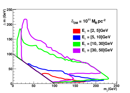
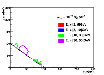
Figure 4: Contours of 95%percent9595\% CL constraint on the mχ~Δmsubscript𝑚~𝜒Δ𝑚m_{\tilde{\chi}}-\Delta{m} plane based on one year of observation of Centaurus A by the Fermi LAT. The colored regions indicate constraints from each energy bin reported by Fermi, and the black dashed line indicates me~=100subscript𝑚~𝑒100m_{\tilde{e}}=100 GeV. The two panels assume different δDMsubscript𝛿DM\delta_{\rm DM}, as indicated.

In Figure 4, we plot the 95%percent9595\% CL bounds in the plane of mχ~subscript𝑚~𝜒m_{\tilde{\chi}} and ΔmΔ𝑚\Delta m, where

ΔmΔ𝑚\displaystyle\Delta m \displaystyle\equiv me~mχ~subscript𝑚~𝑒subscript𝑚~𝜒\displaystyle m_{\tilde{e}}-m_{\tilde{\chi}} (4.3)

is the mass splitting between the neutralino and selectron. The left panel corresponds to δDM=1010Mpc2subscript𝛿DMsuperscript1010subscript𝑀direct-productsuperscriptpc2\delta_{\rm DM}=10^{10}~{}M_{\odot}~{}{\rm pc}^{-2}, and the right to δDM=1011Mpc2subscript𝛿DMsuperscript1011subscript𝑀direct-productsuperscriptpc2\delta_{\rm DM}=10^{11}~{}M_{\odot}~{}{\rm pc}^{-2}. These values correspond to a neutralino annihilation cross section of σv1030similar-todelimited-⟨⟩𝜎𝑣superscript1030\langle\sigma v\rangle\sim 10^{-30} cm3 s-1 (appropriate for a coannihilation scenario) and a black hole lifetime of tBH108similar-tosubscript𝑡BHsuperscript108t_{\rm BH}\sim 10^{8} or 1010superscript101010^{10} years, respectively. We continue to assume a bino neutralino and selectrons which are degenerate in mass. Since the optimal energy bin for the search varies with mχ~subscript𝑚~𝜒m_{\tilde{\chi}} and me~subscript𝑚~𝑒m_{\tilde{e}}, we derive the ruled out region from each energy bin independently, as indicated on the figure. We find that the largest resolving power comes from the highest energy bins, but nevertheless the lower energy bins provide interesting constraints, and a combined shape analysis would probably do a little better than treating each bin independently. The black dashed line on each panel indicates the line of me~100subscript𝑚~𝑒100m_{\tilde{e}}\geq 100 GeV, roughly the bound from LEP-II null searches [24]. There are no current LHC bounds on slepton masses and what they turn out to be will ultimately depend on the LHC performance. For comparison, the theoretical study in Ref. [14] concluded that the LHC at s=14𝑠14\sqrt{s}=14 TeV and with 100similar-toabsent100\sim 100 fb-1 has sensitivity for slepton masses around 100 GeV, provided the mass splitting is larger than about Δm=20Δ𝑚20\Delta m=20 GeV.

5 Conclusions and Outlook

Active galactic nuclei are among the most energetic natural accelerators in the Universe. They are also located in regions rich with dark matter, and provide a great opportunity to study the high energy interactions of WIMPs with SM particles. In this paper, we have estimated the regions of MSSM parameter space which can be probed from Fermi observations. We find that there is greatest sensitivity for models with low annihilation cross sections and nearly degenerate sleptons – as occurs in coannihilation regions of the MSSM, where sleptons are active during freeze-out. Indeed, sleptons are very challenging to discover at the LHC under ideal circumstances, and almost impossible when nearly degenerate with the lightest supersymmetry particle. Observations of the gamma rays from AGNs can help cover an interesting and important gap in LHC coverage of MSSM parameter space. Analogously, one can study the scattering process between dark matter and AGN jets consisting of protons, although the rates at the highest energies will be suppressed by the parton distribution functions; we leave this direction for future work.

Ultimately, the limiting factors in utilizing these naturally occurring accelerators as probes of the property of dark matter are the uncertainties in the properties of the AGNs themselves and the dark matter environment around them. These uncertainties can be mitigated by further observations, to help pin down the underlying properties of the jet, and observation of the dynamics of the surrounding stars and gas to better constrain the gravitational dynamics. The MSSM signal considered here also leads to a distinctive feature in the gamma ray spectrum, which could be exploited with more statistics to minimize the dependence on the unknown background emission. Ultimately, if the particle properties of dark matter can be pinned down more precisely using data from the LHC or direct or indirect dark matter detection experiments, one could even turn the process around and use collisions between jets and the WIMPs to learn about the astrophysics of these fascinating systems.

6 Acknowledgements

T. Tait is glad to acknowledge conversations with L. Costamente, S. Profumo, and L. Ubaldi, and the hospitality of the SLAC theory group, for their generosity during his many visits. The work of AR and JH is supported in part by NSF grants PHY-0653656 and PHY-0709742. The work of TMPT is supported in part by NSF grant PHY-0970171.

Appendix A Matrix Elements for eχ~eχ~γsuperscript𝑒~𝜒superscript𝑒~𝜒𝛾e^{-}\tilde{\chi}\rightarrow e^{-}\tilde{\chi}\gamma

In this appendix, we summarize the full expression for the amplitude squared for the process eχ~eχ~γsuperscript𝑒~𝜒superscript𝑒~𝜒𝛾e^{-}\tilde{\chi}\rightarrow e^{-}\tilde{\chi}\gamma. We begin with some notations,

αeffsubscript𝛼eff\displaystyle\alpha_{\mbox{\tiny{eff}}} =\displaystyle= 4παEM(aL4+aR4);4𝜋subscript𝛼EMsuperscriptsubscript𝑎L4superscriptsubscript𝑎R4\displaystyle 4\pi\alpha_{\mbox{\tiny{EM}}}(a_{\mbox{\tiny{L}}}^{4}+a_{\mbox{\tiny{R}}}^{4})\;;
s𝑠\displaystyle s =\displaystyle= (p1+p2)2;superscriptsubscript𝑝1subscript𝑝22\displaystyle(p_{1}+p_{2})^{2}\;;
ssuperscript𝑠\displaystyle s^{\prime} =\displaystyle= (p1+p2)2;superscriptsuperscriptsubscript𝑝1superscriptsubscript𝑝22\displaystyle(p_{1}^{\prime}+p_{2}^{\prime})^{2}\;;
u𝑢\displaystyle u =\displaystyle= (p1p2)2;superscriptsubscript𝑝1superscriptsubscript𝑝22\displaystyle(p_{1}-p_{2}^{\prime})^{2}\;;
usuperscript𝑢\displaystyle u^{\prime} =\displaystyle= (p2p1)2;superscriptsubscript𝑝2superscriptsubscript𝑝12\displaystyle(p_{2}-p_{1}^{\prime})^{2}\;;
E1ssubscript𝐸1𝑠\displaystyle E_{1s} =\displaystyle= (s+mχ~2me2)/(2s);𝑠superscriptsubscript𝑚~𝜒2superscriptsubscript𝑚𝑒22𝑠\displaystyle(s+m_{\tilde{\chi}}^{2}-m_{e}^{2})/(2\sqrt{s})\;;
E2ssubscript𝐸2𝑠\displaystyle E_{2s} =\displaystyle= sE1s;𝑠subscript𝐸1𝑠\displaystyle\sqrt{s}-E_{1s}\;;
E1ssubscript𝐸1superscript𝑠\displaystyle E_{1s^{\prime}} =\displaystyle= (s+mχ~2me2)/(2s);superscript𝑠superscriptsubscript𝑚~𝜒2superscriptsubscript𝑚𝑒22superscript𝑠\displaystyle(s^{\prime}+m_{\tilde{\chi}}^{2}-m_{e}^{2})/(2\sqrt{s^{\prime}})\;;
E2ssubscript𝐸2superscript𝑠\displaystyle E_{2s^{\prime}} =\displaystyle= sE1s;superscript𝑠subscript𝐸1superscript𝑠\displaystyle\sqrt{s^{\prime}}-E_{1s^{\prime}}\;;
rssubscript𝑟𝑠\displaystyle r_{s} =\displaystyle= (s(me+mχ~)2)(s(mχ~me)2)/(2s);𝑠superscriptsubscript𝑚𝑒subscript𝑚~𝜒2𝑠superscriptsubscript𝑚~𝜒subscript𝑚𝑒22𝑠\displaystyle\sqrt{(s-(m_{e}+m_{\tilde{\chi}})^{2})(s-(m_{\tilde{\chi}}-m_{e})^{2})}/(2\sqrt{s})\;;
rssubscript𝑟superscript𝑠\displaystyle r_{s^{\prime}} =\displaystyle= (s(me+mχ~)2)(s(mχ~me)2)/(2s);superscript𝑠superscriptsubscript𝑚𝑒subscript𝑚~𝜒2superscript𝑠superscriptsubscript𝑚~𝜒subscript𝑚𝑒22superscript𝑠\displaystyle\sqrt{(s^{\prime}-(m_{e}+m_{\tilde{\chi}})^{2})(s^{\prime}-(m_{\tilde{\chi}}-m_{e})^{2})}/(2\sqrt{s^{\prime}})\;;
Γ1subscriptΓ1\displaystyle\Gamma_{1} =\displaystyle= ((aL2+aR2)(E1sE2s+rs2)rs)/(4πme~s);superscriptsubscript𝑎L2superscriptsubscript𝑎R2subscript𝐸1𝑠subscript𝐸2𝑠superscriptsubscript𝑟𝑠2subscript𝑟𝑠4𝜋subscript𝑚~𝑒𝑠\displaystyle((a_{\mbox{\tiny{L}}}^{2}+a_{\mbox{\tiny{R}}}^{2})(E_{1s}E_{2s}+r_{s}^{2})r_{s})/(4\pi m_{\tilde{e}}\sqrt{s});
Γ2subscriptΓ2\displaystyle\Gamma_{2} =\displaystyle= ((aL2+aR2)(E1sE2s+rs2)rs)/(4πme~s);superscriptsubscript𝑎L2superscriptsubscript𝑎R2subscript𝐸1superscript𝑠subscript𝐸2superscript𝑠superscriptsubscript𝑟superscript𝑠2subscript𝑟superscript𝑠4𝜋subscript𝑚~𝑒superscript𝑠\displaystyle((a_{\mbox{\tiny{L}}}^{2}+a_{\mbox{\tiny{R}}}^{2})(E_{1s^{\prime}}E_{2s^{\prime}}+r_{s^{\prime}}^{2})r_{s^{\prime}})/(4\pi m_{\tilde{e}}\sqrt{s^{\prime}})\;;
ΣssubscriptΣ𝑠\displaystyle\Sigma_{s} =\displaystyle= sme~2ime~Γ1;𝑠superscriptsubscript𝑚~𝑒2𝑖subscript𝑚~𝑒subscriptΓ1\displaystyle s-m_{\tilde{e}}^{2}-i\,m_{\tilde{e}}\Gamma_{1}\;;
ΣssubscriptΣsuperscript𝑠\displaystyle\Sigma_{s^{\prime}} =\displaystyle= sme~2ime~Γ2;superscript𝑠superscriptsubscript𝑚~𝑒2𝑖subscript𝑚~𝑒subscriptΓ2\displaystyle s^{\prime}-m_{\tilde{e}}^{2}-i\,m_{\tilde{e}}\Gamma_{2}\;;
ΣusubscriptΣ𝑢\displaystyle\Sigma_{u} =\displaystyle= ume~2;𝑢superscriptsubscript𝑚~𝑒2\displaystyle u-m_{\tilde{e}}^{2}\;;
ΣusubscriptΣsuperscript𝑢\displaystyle\Sigma_{u^{\prime}} =\displaystyle= ume~2;superscript𝑢superscriptsubscript𝑚~𝑒2\displaystyle u^{\prime}-m_{\tilde{e}}^{2}\;;
f3subscript𝑓3\displaystyle f_{3} =\displaystyle= 1+i(me~(Γ1Γ2))/(2((p1+p2)r));1𝑖subscript𝑚~𝑒subscriptΓ1subscriptΓ22subscript𝑝1subscript𝑝2𝑟\displaystyle 1+i(m_{\tilde{e}}(\Gamma_{1}-\Gamma_{2}))/(2((p_{1}+p_{2})\cdot r))\;;
|Σs|2superscriptsubscriptΣ𝑠2\displaystyle|\Sigma_{s}|^{2} =\displaystyle= (sme~2)2+(me~Γ1)2;superscript𝑠superscriptsubscript𝑚~𝑒22superscriptsubscript𝑚~𝑒subscriptΓ12\displaystyle(s-m_{\tilde{e}}^{2})^{2}+(m_{\tilde{e}}~{}\Gamma_{1})^{2}\;;
|Σs|2superscriptsubscriptΣsuperscript𝑠2\displaystyle|\Sigma_{s^{\prime}}|^{2} =\displaystyle= (sme~2)2+(me~Γ2)2.superscriptsuperscript𝑠superscriptsubscript𝑚~𝑒22superscriptsubscript𝑚~𝑒subscriptΓ22\displaystyle(s^{\prime}-m_{\tilde{e}}^{2})^{2}+(m_{\tilde{e}}~{}\Gamma_{2})^{2}\;. (A.1)

Here p1,p1,p2,p2,rsubscript𝑝1superscriptsubscript𝑝1subscript𝑝2superscriptsubscript𝑝2𝑟p_{1}\,,p_{1}^{\prime}\,,p_{2}\,,p_{2}^{\prime}\,,r are the four-vectors for the momenta of the incoming and outgoing dark matter particles (neutralino), incoming and outgoing electrons and photon. E1ssubscript𝐸1𝑠E_{1s}, E2ssubscript𝐸2𝑠E_{2s}, E1ssubscript𝐸1superscript𝑠E_{1s^{\prime}}, and E2ssubscript𝐸2superscript𝑠E_{2s^{\prime}} are the energies of the initial and final neutralino and electron in the lab frame where the initial neutralino is at rest. The s𝑠s and ssuperscript𝑠s^{\prime} subscripts correspond to the s𝑠s and ssuperscript𝑠s^{\prime} diagrams, respectively. ΓisubscriptΓ𝑖\Gamma_{i} are the momentum dependent decay widths and ΣssubscriptΣ𝑠\Sigma_{s}, ΣssubscriptΣsuperscript𝑠\Sigma_{s^{\prime}} and ΣusubscriptΣ𝑢\Sigma_{u}, ΣusubscriptΣsuperscript𝑢\Sigma_{u^{\prime}} are the propagators in the s𝑠s- and u𝑢u-channels. f3subscript𝑓3f_{3} is the modified vertex factor in amplitude M3subscript𝑀3M_{3} which insures gauge invariance, see appendix B. The squared amplitudes, including the interference terms, are:

|M1|2=[αeff(p1r)(p1p2)]/[|Σs|2(p2r)];|M2|2=[αeff(p1r)(p1p2)]/[|Σs|2((p2r)me22)];|M3|2=[4αeff(p1p2)(p1p2)(2(p1p2)(p1r)(p2r)+mχ~2)|f3|2]/[|Σs|2|Σs|2];2Re(M1M2)=Re[αeffΣsΣs(p2r)((p2r)me2/2)((p1p2)(p1r)(p2r)(p1p2)(p1r)(p1p2)+(p1p2)(p2r)23(p1p2)(p2r)(p1p2)+2(p1p2)(p1p2)2(p2p2)(p1r)2(p2p2)(p1r)(p2r)+(p2p2)(p1r)(p1p2)(p2p2)(p2r)(p1p2)(p1r)2(p1p2)2(p1r)(p2r)(p1p2)+3(p1r)(p1p2)2(p2r)2(p1p2)+3(p2r)(p1p2)22(p1p2)3)];2Re(M1M3)=Re[2αefff3|Σs|2Σs(p2r)(2(p1r)2(p2p1)+3(p1r)(p2r)(p1p2)(p1r)(p2r)mχ~24(p1r)(p2p1)2+(p2r)2(p1p2)(p2r)2mχ~23(p2r)(p2p1)2+(p2r)(p1p2)mχ~2+2(p2p1)3)];2Re(M2M3)=Re[2αefff3|Σs|2Σs((p2r)me2/2)((p1p2)(p1r)(p1p2)+(p1p2)(p2r)(p1p2)(p1p2)(p2p1)2(p1p2)(p1p2)mχ~2+(p2p2)(p1r)(p1p2)+(p2p2)(p2r)(p1p2)(p2p2)(p1p2)2(p2p2)(p2p1)mχ~2+(p1r)2(p1p2)+2(p1r)(p2r)(p1p2)4(p1r)(p1p2)2(p1r)(p1p2)mχ~2+(p2r)2(p1p2)4(p2r)(p1p2)2(p2r)(p1p2)mχ~2+3(p1p2)3+(p1p2)2mχ~2)];\begin{array}[]{lll}|M_{1}|^{2}&=&[\alpha_{\mbox{\tiny{eff}}}(p_{1}\cdot r)(p_{1}^{\prime}\cdot p_{2}^{\prime})]/[|\Sigma_{s^{\prime}}|^{2}(p_{2}\cdot r)]\;;\\ |M_{2}|^{2}&=&[\alpha_{\mbox{\tiny{eff}}}(p_{1}^{\prime}\cdot r)(p_{1}\cdot p_{2})]/[|\Sigma_{s}|^{2}((p_{2}^{\prime}\cdot r)-\frac{m_{e}^{2}}{2})]\;;\\ |M_{3}|^{2}&=&[-4\alpha_{\mbox{\tiny{eff}}}(p_{1}\cdot p_{2})(p_{1}^{\prime}\cdot p_{2}^{\prime})(2(p_{1}\cdot p_{2})-(p_{1}\cdot r)-(p_{2}\cdot r)+m_{\tilde{\chi}}^{2})|f_{3}|^{2}]/[|\Sigma_{s}|^{2}|\Sigma_{s^{\prime}}|^{2}]\;;\\ 2Re(M_{1}M_{2}^{\dagger})&=&Re\biggl{[}\frac{-\alpha_{\mbox{\tiny{eff}}}}{\Sigma_{s^{\prime}}\Sigma_{s}^{*}(p_{2}\cdot r)((p_{2}^{\prime}\cdot r)-m_{e}^{2}/2)}\biggl{(}(p_{1}\cdot p_{2}^{\prime})(p_{1}\cdot r)(p_{2}\cdot r)-(p_{1}\cdot p_{2}^{\prime})(p_{1}\cdot r)(p_{1}\cdot p_{2})\\ &&{}+(p_{1}\cdot p_{2}^{\prime})(p_{2}\cdot r)^{2}-3(p_{1}\cdot p_{2}^{\prime})(p_{2}\cdot r)(p_{1}\cdot p_{2})+2(p_{1}\cdot p_{2}^{\prime})(p_{1}\cdot p_{2})^{2}\\ &&{}-(p_{2}\cdot p_{2}^{\prime})(p_{1}\cdot r)^{2}-(p_{2}\cdot p_{2}^{\prime})(p_{1}\cdot r)(p_{2}\cdot r)+(p_{2}\cdot p_{2}^{\prime})(p_{1}\cdot r)(p_{1}\cdot p_{2})\\ &&{}-(p_{2}\cdot p_{2}^{\prime})(p_{2}\cdot r)(p_{1}\cdot p_{2})-(p_{1}\cdot r)^{2}(p_{1}\cdot p_{2})-2(p_{1}\cdot r)(p_{2}\cdot r)(p_{1}\cdot p_{2})\\ &&{}+3(p_{1}\cdot r)(p_{1}\cdot p_{2})^{2}-(p_{2}\cdot r)^{2}(p_{1}\cdot p_{2})+3(p_{2}\cdot r)(p_{1}\cdot p_{2})^{2}-2(p_{1}\cdot p_{2})^{3}\biggr{)}\biggr{]}\;;\\ 2Re(M_{1}M_{3}^{\dagger})&=&Re\biggl{[}\frac{2\alpha_{\mbox{\tiny{eff}}}f_{3}}{|\Sigma_{s^{\prime}}|^{2}\Sigma_{s}^{*}(p_{2}\cdot r)}\biggl{(}2(p_{1}\cdot r)^{2}(p_{2}\cdot p_{1})+3(p_{1}\cdot r)(p_{2}\cdot r)(p_{1}\cdot p_{2})\\ &&{}-(p_{1}\cdot r)(p_{2}\cdot r)m_{\tilde{\chi}}^{2}-4(p_{1}\cdot r)(p_{2}\cdot p_{1})^{2}+(p_{2}\cdot r)^{2}(p_{1}\cdot p_{2})\\ &&{}-(p_{2}\cdot r)^{2}m_{\tilde{\chi}}^{2}-3(p_{2}\cdot r)(p_{2}\cdot p_{1})^{2}+(p_{2}\cdot r)(p_{1}\cdot p_{2})m_{\tilde{\chi}}^{2}+2(p_{2}\cdot p_{1})^{3}\biggr{)}\biggr{]}\;;\\ 2Re(M_{2}M_{3}^{\dagger})&=&Re\biggl{[}\frac{-2\alpha_{\mbox{\tiny{eff}}}f_{3}}{|\Sigma_{s}|^{2}\Sigma_{s^{\prime}}^{*}((p_{2}^{\prime}\cdot r)-m_{e}^{2}/2)}\biggl{(}(p_{1}\cdot p_{2}^{\prime})(p_{1}\cdot r)(p_{1}\cdot p_{2})+(p_{1}\cdot p_{2}^{\prime})(p_{2}\cdot r)(p_{1}\cdot p_{2})\\ &&{}-(p_{1}\cdot p_{2}^{\prime})(p_{2}\cdot p_{1})^{2}-(p_{1}\cdot p_{2}^{\prime})(p_{1}\cdot p_{2})m_{\tilde{\chi}}^{2}+(p_{2}\cdot p_{2}^{\prime})(p_{1}\cdot r)(p_{1}\cdot p_{2})\\ &&{}+(p_{2}\cdot p_{2}^{\prime})(p_{2}\cdot r)(p_{1}\cdot p_{2})-(p_{2}\cdot p_{2}^{\prime})(p_{1}\cdot p_{2})^{2}-(p_{2}\cdot p_{2}^{\prime})(p_{2}\cdot p_{1})m_{\tilde{\chi}}^{2}\\ &&{}+(p_{1}\cdot r)^{2}(p_{1}\cdot p_{2})+2(p_{1}\cdot r)(p_{2}\cdot r)(p_{1}\cdot p_{2})-4(p_{1}\cdot r)(p_{1}\cdot p_{2})^{2}\\ &&{}-(p_{1}\cdot r)(p_{1}\cdot p_{2})m_{\tilde{\chi}}^{2}+(p_{2}\cdot r)^{2}(p_{1}\cdot p_{2})-4(p_{2}\cdot r)(p_{1}\cdot p_{2})^{2}\\ &&{}-(p_{2}\cdot r)(p_{1}\cdot p_{2})m_{\tilde{\chi}}^{2}+3(p_{1}\cdot p_{2})^{3}+(p_{1}\cdot p_{2})^{2}m_{\tilde{\chi}}^{2}\biggr{)}\biggr{]}\;;\end{array} (A.2)
|M4|2=[αeff(p1r)(p1p2)]/[Σu2(p2r)];|M5|2=[αeff(p1r)(p1p2)]/[Σu2(p2rme2/2)];|M6|2=[4αeff(p1p2)(p2p1)((p2p1)+(p1p2)mχ~2)]/[Σu2Σu2]2Re(M4M5)=Re[αeffΣuΣu(p2r)((p2r)me2/2)(2(p1p2)2(p2p2)+(p1p2)2(p2r)(p1p2)2(p1p2)+(p1p2)(p2p2)(p1r)+(p2p1)3(p1p2)(p2p2)(p2r)(p1p2)(p1r)(p2p1)(p1p2)(p2r)2+(p1p2)(p2r)(p1p2)(p2p2)2(p1r)+(p2p2)2(p1p2)(p2p2)(p1r)(p2r)+2(p2p2)(p1r)(p2p1)+2(p2p2)(p2r)(p1p2)2(p2p2)(p2p1)2+(p1r)(p2r)(p1p2)(p1r)(p1p2)2+(p2r)2(p1p2)2(p2r)(p1p2)2)];2Re(M4M6)=Re[2αeffΣu2Σu(p2r)(2(p1p2)2(p2p2)+2(p1p2)2(p2r)2(p1p2)2(p1p2)(p1p2)(p2p2)(p2r)(p1p2)(p2r)2+(p1p2)(p2r)(p1p2)(p1p2)(p2r)mχ~2)];2Re(M5M6)=Re[2αeffΣu2Σu2((p2r)me2/2)((p1p2)2(p2p2)+(p1p2)2(p2r)(p1p2)2(p1p2)(p1p2)(p2p2)2+(p1p2)(p2p2)(p1r)2(p1p2)(p2p2)(p2r)+2(p1p2)(p2p2)(p1p2)(p1p2)(p2p2)mχ~2+(p1p2)(p1r)(p2r)(p1p2)(p1r)(p1p2)(p1p2)(p2r)2+2(p1p2)(p2r)(p1p2)(p1p2)(p2r)mχ~2(p1p2)(p1p2)2+(p1p2)(p1p2)mχ~2(p2p2)2mχ~2(p2p2)(p1r)mχ~22(p2p2)(p2r)mχ~2+2(p2p2)(p1p2)mχ~2(p1r)(p2r)mχ~2+(p1r)(p1p2)mχ~2(p2r)2mχ~2+2(p2r)(p1p2)mχ~2(p1p2)2mχ~2)];\begin{array}[]{lll}|M_{4}|^{2}&=&[\alpha_{\mbox{\tiny{eff}}}(p_{1}^{\prime}\cdot r)(p_{1}\cdot p_{2}^{\prime})]/[\Sigma_{u}^{2}(p_{2}\cdot r)]\;;\\ |M_{5}|^{2}&=&[\alpha_{\mbox{\tiny{eff}}}(p_{1}\cdot r)(p_{1}^{\prime}\cdot p_{2})]/[\Sigma_{u^{\prime}}^{2}(p_{2}^{\prime}\cdot r-m_{e}^{2}/2)]\;;\\ |M_{6}|^{2}&=&[4\alpha_{\mbox{\tiny{eff}}}(p_{1}\cdot p_{2}^{\prime})(p_{2}\cdot p_{1}^{\prime})((p_{2}\cdot p_{1}^{\prime})+(p_{1}\cdot p_{2}^{\prime})-m_{\tilde{\chi}}^{2})]/[\Sigma_{u}^{2}\Sigma_{u^{\prime}}^{2}]\\ 2Re(M_{4}M_{5}^{\dagger})&=&Re\biggl{[}\frac{\alpha_{\mbox{\tiny{eff}}}}{\Sigma_{u}\Sigma_{u^{\prime}}(p_{2}\cdot r)((p_{2}^{\prime}\cdot r)-m_{e}^{2}/2)}\biggl{(}2(p_{1}\cdot p_{2}^{\prime})^{2}(p_{2}\cdot p_{2}^{\prime})+(p_{1}\cdot p_{2}^{\prime})^{2}(p_{2}\cdot r)\\ &&{}-(p_{1}\cdot p_{2}^{\prime})^{2}(p_{1}\cdot p_{2})+(p_{1}\cdot p_{2}^{\prime})(p_{2}\cdot p_{2}^{\prime})(p_{1}\cdot r)+(p_{2}\cdot p_{1})^{3}\\ &&{}-(p_{1}\cdot p_{2}^{\prime})(p_{2}\cdot p_{2}^{\prime})(p_{2}\cdot r)-(p_{1}\cdot p_{2}^{\prime})(p_{1}\cdot r)(p_{2}\cdot p_{1})-(p_{1}\cdot p_{2}^{\prime})(p_{2}\cdot r)^{2}\\ &&{}+(p_{1}\cdot p_{2}^{\prime})(p_{2}\cdot r)(p_{1}\cdot p_{2})-(p_{2}\cdot p_{2}^{\prime})^{2}(p_{1}\cdot r)+(p_{2}\cdot p_{2}^{\prime})^{2}(p_{1}\cdot p_{2})\\ &&{}-(p_{2}\cdot p_{2}^{\prime})(p_{1}\cdot r)(p_{2}\cdot r)+2(p_{2}\cdot p_{2}^{\prime})(p_{1}\cdot r)(p_{2}\cdot p_{1})+2(p_{2}\cdot p_{2}^{\prime})(p_{2}\cdot r)(p_{1}\cdot p_{2})\\ &&{}-2(p_{2}\cdot p_{2}^{\prime})(p_{2}\cdot p_{1})^{2}+(p_{1}\cdot r)(p_{2}\cdot r)(p_{1}\cdot p_{2})-(p_{1}\cdot r)(p_{1}\cdot p_{2})^{2}\\ &&{}+(p_{2}\cdot r)^{2}(p_{1}\cdot p_{2})-2(p_{2}\cdot r)(p_{1}\cdot p_{2})^{2}\biggr{)}\biggr{]}\;;\\ 2Re(M_{4}M_{6}^{\dagger})&=&Re\biggl{[}\frac{2\alpha_{\mbox{\tiny{eff}}}}{\Sigma_{u}^{2}\Sigma_{u^{\prime}}(p_{2}\cdot r)}\biggl{(}2(p_{1}\cdot p_{2}^{\prime})^{2}(p_{2}\cdot p_{2}^{\prime})+2(p_{1}\cdot p_{2}^{\prime})^{2}(p_{2}\cdot r)\\ &&{}-2(p_{1}\cdot p_{2}^{\prime})^{2}(p_{1}\cdot p_{2})-(p_{1}\cdot p_{2}^{\prime})(p_{2}\cdot p_{2}^{\prime})(p_{2}\cdot r)-(p_{1}\cdot p_{2}^{\prime})(p_{2}\cdot r)^{2}\\ &&{}+(p_{1}\cdot p_{2}^{\prime})(p_{2}\cdot r)(p_{1}\cdot p_{2})-(p_{1}\cdot p_{2}^{\prime})(p_{2}\cdot r)m_{\tilde{\chi}}^{2}\biggr{)}\biggr{]}\;;\\ 2Re(M_{5}M_{6}^{\dagger})&=&Re\biggl{[}\frac{-2\alpha_{\mbox{\tiny{eff}}}}{\Sigma_{u}^{2}\Sigma_{u^{\prime}}^{2}((p_{2}^{\prime}\cdot r)-m_{e}^{2}/2)}\biggl{(}(p_{1}\cdot p_{2}^{\prime})^{2}(p_{2}\cdot p_{2}^{\prime})+(p_{1}\cdot p_{2}^{\prime})^{2}(p_{2}\cdot r)\\ &&{}-(p_{1}\cdot p_{2}^{\prime})^{2}(p_{1}\cdot p_{2})-(p_{1}\cdot p_{2}^{\prime})(p_{2}\cdot p_{2}^{\prime})^{2}+(p_{1}\cdot p_{2}^{\prime})(p_{2}\cdot p_{2}^{\prime})(p_{1}\cdot r)\\ &&{}-2(p_{1}\cdot p_{2}^{\prime})(p_{2}\cdot p_{2}^{\prime})(p_{2}\cdot r)+2(p_{1}\cdot p_{2}^{\prime})(p_{2}\cdot p_{2}^{\prime})(p_{1}\cdot p_{2})-(p_{1}\cdot p_{2}^{\prime})(p_{2}\cdot p_{2}^{\prime})m_{\tilde{\chi}}^{2}\\ &&{}+(p_{1}\cdot p_{2}^{\prime})(p_{1}\cdot r)(p_{2}\cdot r)-(p_{1}\cdot p_{2}^{\prime})(p_{1}\cdot r)(p_{1}\cdot p_{2})-(p_{1}\cdot p_{2}^{\prime})(p_{2}\cdot r)^{2}\\ &&{}+2(p_{1}\cdot p_{2}^{\prime})(p_{2}\cdot r)(p_{1}\cdot p_{2})-(p_{1}\cdot p_{2}^{\prime})(p_{2}\cdot r)m_{\tilde{\chi}}^{2}-(p_{1}\cdot p_{2}^{\prime})(p_{1}\cdot p_{2})^{2}\\ &&{}+(p_{1}\cdot p_{2}^{\prime})(p_{1}\cdot p_{2})m_{\tilde{\chi}}^{2}-(p_{2}\cdot p_{2}^{\prime})^{2}m_{\tilde{\chi}}^{2}-(p_{2}\cdot p_{2}^{\prime})(p_{1}\cdot r)m_{\tilde{\chi}}^{2}\\ &&{}-2(p_{2}\cdot p_{2}^{\prime})(p_{2}\cdot r)m_{\tilde{\chi}}^{2}+2(p_{2}\cdot p_{2}^{\prime})(p_{1}\cdot p_{2})m_{\tilde{\chi}}^{2}-(p_{1}\cdot r)(p_{2}\cdot r)m_{\tilde{\chi}}^{2}\\ &&{}+(p_{1}\cdot r)(p_{1}\cdot p_{2})m_{\tilde{\chi}}^{2}-(p_{2}\cdot r)^{2}m_{\tilde{\chi}}^{2}+2(p_{2}\cdot r)(p_{1}\cdot p_{2})m_{\tilde{\chi}}^{2}-(p_{1}\cdot p_{2})^{2}m_{\tilde{\chi}}^{2}\biggr{)}\biggr{]}\;;\end{array} (A.3)
2Re(M1M4)=Re[αeffmχ~2ΣsΣu(p2r)((p1p2)+(p2p2)+(p1r)+(p2r)(p1p2))];2Re(M1M5)=Re[αeffmχ~2ΣsΣu(p2r)((p2r)me2/2)((p1p2)(p2p2)+(p2p2)(p1r)(p2p2)(p1p2))];2Re(M1M6)=Re[αeffmχ~2ΣsΣuΣu(p2r)(2(p1p2)(p2p2)+(p1p2)(p2r)(p1p2)(p1p2)+(p2p2)(p1r)+(p2p2)(p2r)(p2p2)(p1p2)(p1r)(p1p2)(p2r)(p1p2)+(p1p2)2)];2Re(M4M2)=Re[αeffmχ~2ΣuΣs(p2r)((p2r)me2/2)((p1p2)(p2p2)+(p2p2)(p1r)(p2p2)(p1p2))];2Re(M2M5)=Re[[αeffmχ~2(p2r)]/[ΣsΣu((p2r)me2/2)]];2Re(M2M6)=Re[αeffmχ~2ΣsΣuΣu((p2r)me2/2)((p1p2)(p2p2)+(p1p2)(p2r)(p1p2)(p1p2)(p2p2)2(p2p2)(p2r)(p1r)(p1p2)(p2r)(p1p2)+(p1p2)2)];2Re(M4M3)=Re[αeffmχ~2f3ΣuΣsΣs(p2r)((p1p2)(p2r)(p1p2)(p1p2)(p2p2)(p1r)(p2p2)(p2r)+(p2p2)(p1p2)(p1r)(p1p2)(p2r)(p1p2)+(p1p2)2)];2Re(M5M3)=Re[αeffmχ~2f3ΣuΣsΣs((p2r)me2/2)((p1p2)(p2p2)+(p1p2)(p2r)(p1p2)(p1p2)+(p2p2)2+(p2p2)(p2r)(p1r)(p1p2)(p2r)(p1p2)+(p1p2)2)];2Re(M3M6)=Re[2αeffmχ~2f3ΣsΣsΣuΣu((p1p2)(p2p2)+(p2p2)2+(p2p2)(p1r)(p2p2)(p1p2)2(p2p2)mχ~2)].\begin{array}[]{lll}2Re(M_{1}M_{4}^{\dagger})&=&Re\biggl{[}\frac{\alpha_{\mbox{\tiny{eff}}}\,m_{\tilde{\chi}}^{2}}{\Sigma_{s^{\prime}}\Sigma_{u}(p_{2}\cdot r)}\biggl{(}(p_{1}\cdot p_{2}^{\prime})+(p_{2}\cdot p_{2}^{\prime})+(p_{1}\cdot r)+(p_{2}\cdot r)-(p_{1}\cdot p_{2})\biggr{)}\biggr{]}\;;\\ 2Re(M_{1}M_{5}^{\dagger})&=&Re\biggl{[}\frac{-\alpha_{\mbox{\tiny{eff}}}\,m_{\tilde{\chi}}^{2}}{\Sigma_{s^{\prime}}\Sigma_{u^{\prime}}(p_{2}\cdot r)((p_{2}^{\prime}\cdot r)-m_{e}^{2}/2)}\biggl{(}(p_{1}\cdot p_{2}^{\prime})(p_{2}\cdot p_{2}^{\prime})+(p_{2}\cdot p_{2}^{\prime})(p_{1}\cdot r)-(p_{2}\cdot p_{2}^{\prime})(p_{1}\cdot p_{2})\biggr{)}\biggr{]}\;;\\ 2Re(M_{1}M_{6}^{\dagger})&=&Re\biggl{[}\frac{-\alpha_{\mbox{\tiny{eff}}}\,m_{\tilde{\chi}}^{2}}{\Sigma_{s^{\prime}}\Sigma_{u^{\prime}}\Sigma_{u}(p_{2}\cdot r)}\biggl{(}2(p_{1}\cdot p_{2}^{\prime})(p_{2}\cdot p_{2}^{\prime})+(p_{1}\cdot p_{2}^{\prime})(p_{2}\cdot r)\\ &&{}-(p_{1}\cdot p_{2}^{\prime})(p_{1}\cdot p_{2})+(p_{2}\cdot p_{2}^{\prime})(p_{1}\cdot r)+(p_{2}\cdot p_{2}^{\prime})(p_{2}\cdot r)\\ &&{}-(p_{2}\cdot p_{2}^{\prime})(p_{1}\cdot p_{2})-(p_{1}\cdot r)(p_{1}\cdot p_{2})-(p_{2}\cdot r)(p_{1}\cdot p_{2})+(p_{1}\cdot p_{2})^{2}\biggr{)}\biggr{]}\;;\\ 2Re(M_{4}M_{2}^{\dagger})&=&Re\biggl{[}\frac{-\alpha_{\mbox{\tiny{eff}}}\,m_{\tilde{\chi}}^{2}}{\Sigma_{u}\Sigma_{s}^{*}(p_{2}\cdot r)((p_{2}^{\prime}\cdot r)-m_{e}^{2}/2)}\biggl{(}(p_{1}\cdot p_{2}^{\prime})(p_{2}\cdot p_{2}^{\prime})+(p_{2}\cdot p_{2}^{\prime})(p_{1}\cdot r)-(p_{2}\cdot p_{2}^{\prime})(p_{1}\cdot p_{2})\biggr{)}\biggr{]}\;;\\ 2Re(M_{2}M_{5}^{\dagger})&=&Re\biggl{[}[\alpha_{\mbox{\tiny{eff}}}\,m_{\tilde{\chi}}^{2}(p_{2}\cdot r)]/[\Sigma_{s}\Sigma_{u^{\prime}}((p_{2}^{\prime}\cdot r)-m_{e}^{2}/2)]\biggr{]}\;;\\ 2Re(M_{2}M_{6}^{\dagger})&=&Re\biggl{[}\frac{\alpha_{\mbox{\tiny{eff}}}\,m_{\tilde{\chi}}^{2}}{\Sigma_{s}\Sigma_{u}\Sigma_{u^{\prime}}((p_{2}^{\prime}\cdot r)-m_{e}^{2}/2)}\biggl{(}(p_{1}\cdot p_{2}^{\prime})(p_{2}\cdot p_{2}^{\prime})+(p_{1}\cdot p_{2}^{\prime})(p_{2}\cdot r)\\ &&{}-(p_{1}\cdot p_{2}^{\prime})(p_{1}\cdot p_{2})-(p_{2}\cdot p_{2}^{\prime})^{2}-(p_{2}\cdot p_{2}^{\prime})(p_{2}\cdot r)\\ &&{}-(p_{1}\cdot r)(p_{1}\cdot p_{2})-(p_{2}\cdot r)(p_{1}\cdot p_{2})+(p_{1}\cdot p_{2})^{2}\biggr{)}\biggr{]};\\ 2Re(M_{4}M_{3}^{\dagger})&=&Re\biggl{[}\frac{\alpha_{\mbox{\tiny{eff}}}\,m_{\tilde{\chi}}^{2}\,f_{3}}{\Sigma_{u}\Sigma_{s}^{*}\Sigma_{s^{\prime}}^{*}(p_{2}\cdot r)}\biggl{(}(p_{1}\cdot p_{2}^{\prime})(p_{2}\cdot r)-(p_{1}\cdot p_{2}^{\prime})(p_{1}\cdot p_{2})\\ &&{}-(p_{2}\cdot p_{2}^{\prime})(p_{1}\cdot r)-(p_{2}\cdot p_{2}^{\prime})(p_{2}\cdot r)+(p_{2}\cdot p_{2}^{\prime})(p_{1}\cdot p_{2})\\ &&{}-(p_{1}\cdot r)(p_{1}\cdot p_{2})-(p_{2}\cdot r)(p_{1}\cdot p_{2})+(p_{1}\cdot p_{2})^{2}\biggr{)}\biggr{]};\\ 2Re(M_{5}M_{3}^{\dagger})&=&Re\biggl{[}\frac{-\alpha_{\mbox{\tiny{eff}}}\,m_{\tilde{\chi}}^{2}\,f_{3}}{\Sigma_{u^{\prime}}\Sigma_{s}^{*}\Sigma_{s^{\prime}}^{*}((p_{2}^{\prime}\cdot r)-m_{e}^{2}/2)}\biggl{(}(p_{1}\cdot p_{2}^{\prime})(p_{2}\cdot p_{2}^{\prime})+(p_{1}\cdot p_{2}^{\prime})(p_{2}\cdot r)\\ &&{}-(p_{1}\cdot p_{2}^{\prime})(p_{1}\cdot p_{2})+(p_{2}\cdot p_{2}^{\prime})^{2}+(p_{2}\cdot p_{2}^{\prime})(p_{2}\cdot r)\\ &&{}-(p_{1}\cdot r)(p_{1}\cdot p_{2})-(p_{2}\cdot r)(p_{1}\cdot p_{2})+(p_{1}\cdot p_{2})^{2}\biggr{)}\biggr{]};\\ 2Re(M_{3}M_{6}^{\dagger})&=&Re\biggl{[}\frac{-2\alpha_{\mbox{\tiny{eff}}}\,m_{\tilde{\chi}}^{2}\,f_{3}^{*}}{\Sigma_{s}\Sigma_{s^{\prime}}\Sigma_{u}\Sigma_{u^{\prime}}}\biggl{(}(p_{1}\cdot p_{2}^{\prime})(p_{2}\cdot p_{2}^{\prime})+(p_{2}\cdot p_{2}^{\prime})^{2}\\ &&{}+(p_{2}\cdot p_{2}^{\prime})(p_{1}\cdot r)-(p_{2}\cdot p_{2}^{\prime})(p_{1}\cdot p_{2})-2(p_{2}\cdot p_{2}^{\prime})m_{\tilde{\chi}}^{2}\biggr{)}\biggr{]}\;.\end{array} (A.4)

Appendix B Proof of Gauge Invariance

In this appendix, we verify the invariance of the amplitude under U(1)EM𝑈subscript1EMU(1)_{\rm EM} gauge transformations. We begin with the set of u𝑢u-channel Feynman graphs. The amplitudes of M4,M5subscript𝑀4subscript𝑀5M_{4},M_{5} and M6subscript𝑀6M_{6} can be written as,

M4subscript𝑀4\displaystyle M_{4} =\displaystyle= [χ~¯(p1)(aLPL+aRPR)iγ.(p2r)me(ieγμ)e(p2)]delimited-[]¯~𝜒superscriptsubscript𝑝1subscript𝑎𝐿subscript𝑃𝐿subscript𝑎𝑅subscript𝑃𝑅𝑖formulae-sequence𝛾subscript𝑝2𝑟subscript𝑚𝑒𝑖𝑒superscript𝛾𝜇𝑒subscript𝑝2\displaystyle\biggl{[}\overline{\tilde{\chi}}(p_{1}^{\prime})(a_{L}P_{L}+a_{R}P_{R}){i\over\gamma.(p_{2}-r)-m_{e}}(-ie\gamma^{\mu}){e}(p_{2})\biggr{]}
[e¯(p2)(aLPL+aRPR)χ(p1)][i(p2p1r)2me~2],delimited-[]¯𝑒superscriptsubscript𝑝2subscript𝑎𝐿subscript𝑃𝐿subscript𝑎𝑅subscript𝑃𝑅𝜒subscript𝑝1delimited-[]𝑖superscriptsubscript𝑝2superscriptsubscript𝑝1𝑟2superscriptsubscript𝑚~𝑒2\displaystyle\biggl{[}\bar{e}(p_{2}^{\prime})(a_{L}P_{L}+a_{R}P_{R})\chi(p_{1})\biggr{]}\biggl{[}{i\over(p_{2}-p_{1}^{\prime}-r)^{2}-m_{\tilde{e}}^{2}}\biggr{]}\;,
M5subscript𝑀5\displaystyle M_{5} =\displaystyle= [χ~¯(p1)(aLPL+aRPR)e(p2)][i(p2p1)2me~2]delimited-[]¯~𝜒superscriptsubscript𝑝1subscript𝑎𝐿subscript𝑃𝐿subscript𝑎𝑅subscript𝑃𝑅𝑒subscript𝑝2delimited-[]𝑖superscriptsubscript𝑝2superscriptsubscript𝑝12superscriptsubscript𝑚~𝑒2\displaystyle\biggl{[}\overline{\tilde{\chi}}(p_{1}^{\prime})(a_{L}P_{L}+a_{R}P_{R}){e}(p_{2})\biggr{]}\biggl{[}{i\over(p_{2}-p_{1}^{\prime})^{2}-m_{\tilde{e}}^{2}}\biggr{]}
[e¯(p2)(ieγμ)iγ.(p2+r)me(aLPL+aRPR)χ(p1)],delimited-[]¯𝑒superscriptsubscript𝑝2𝑖𝑒superscript𝛾𝜇𝑖formulae-sequence𝛾superscriptsubscript𝑝2𝑟subscript𝑚𝑒subscript𝑎𝐿subscript𝑃𝐿subscript𝑎𝑅subscript𝑃𝑅𝜒subscript𝑝1\displaystyle\biggl{[}\bar{e}(p_{2}^{\prime})(-ie\gamma^{\mu}){i\over\gamma.(p_{2}^{\prime}+r)-m_{e}}(a_{L}P_{L}+a_{R}P_{R})\chi(p_{1})\biggr{]}\;,
M6subscript𝑀6\displaystyle M_{6} =\displaystyle= [χ~¯(p1)(aLPL+aRPR)e(p2)][e¯(p2)(aLPL+aRPR)χ(p1)]delimited-[]¯~𝜒superscriptsubscript𝑝1subscript𝑎𝐿subscript𝑃𝐿subscript𝑎𝑅subscript𝑃𝑅𝑒subscript𝑝2delimited-[]¯𝑒superscriptsubscript𝑝2subscript𝑎𝐿subscript𝑃𝐿subscript𝑎𝑅subscript𝑃𝑅𝜒subscript𝑝1\displaystyle\biggl{[}\overline{\tilde{\chi}}(p_{1}^{\prime})(a_{L}P_{L}+a_{R}P_{R}){e}(p_{2})\biggr{]}\biggl{[}\bar{e}(p_{2}^{\prime})(a_{L}P_{L}+a_{R}P_{R})\chi(p_{1})\biggr{]} (B.1)
[i(p2p1)2me~2(ie)(2p22p1r)μi(p2p1r)2me~2].delimited-[]𝑖superscriptsubscript𝑝2superscriptsubscript𝑝12superscriptsubscript𝑚~𝑒2𝑖𝑒superscript2subscript𝑝22superscriptsubscript𝑝1𝑟𝜇𝑖superscriptsubscript𝑝2superscriptsubscript𝑝1𝑟2superscriptsubscript𝑚~𝑒2\displaystyle\biggl{[}{i\over(p_{2}-p_{1}^{\prime})^{2}-m_{\tilde{e}}^{2}}(-ie)(2p_{2}-2p_{1}^{\prime}-r)^{\mu}{i\over(p_{2}-p_{1}^{\prime}-r)^{2}-m_{\tilde{e}}^{2}}\biggr{]}\;.

Applying the Ward identity to M4subscript𝑀4M_{4}-M6subscript𝑀6M_{6} individually gives rise to

M4subscript𝑀4\displaystyle M_{4} =\displaystyle= e[χ~¯(p1)(aLPL+aRPR)e(p2)][e¯(p2)(aLPL+aRPR)χ~(p1)][i(p2p1r)2me~2],𝑒delimited-[]¯~𝜒superscriptsubscript𝑝1subscript𝑎𝐿subscript𝑃𝐿subscript𝑎𝑅subscript𝑃𝑅𝑒subscript𝑝2delimited-[]¯𝑒superscriptsubscript𝑝2subscript𝑎𝐿subscript𝑃𝐿subscript𝑎𝑅subscript𝑃𝑅~𝜒subscript𝑝1delimited-[]𝑖superscriptsubscript𝑝2superscriptsubscript𝑝1𝑟2superscriptsubscript𝑚~𝑒2\displaystyle e\biggl{[}\overline{\tilde{\chi}}(p_{1}^{\prime})(a_{L}P_{L}+a_{R}P_{R}){e}(p_{2})\biggr{]}\biggl{[}\bar{e}(p_{2}^{\prime})(a_{L}P_{L}+a_{R}P_{R})\tilde{\chi}(p_{1})\biggr{]}\biggl{[}{i\over(p_{2}-p_{1}^{\prime}-r)^{2}-m_{\tilde{e}}^{2}}\biggr{]}\;,
M5subscript𝑀5\displaystyle M_{5} =\displaystyle= e[χ~¯(p1)(aLPL+aRPR)e(p2)][e¯(p2)(aLPL+aRPR)χ~(p1)][i(p2p1)2me~2],𝑒delimited-[]¯~𝜒superscriptsubscript𝑝1subscript𝑎𝐿subscript𝑃𝐿subscript𝑎𝑅subscript𝑃𝑅𝑒subscript𝑝2delimited-[]¯𝑒superscriptsubscript𝑝2subscript𝑎𝐿subscript𝑃𝐿subscript𝑎𝑅subscript𝑃𝑅~𝜒subscript𝑝1delimited-[]𝑖superscriptsubscript𝑝2superscriptsubscript𝑝12superscriptsubscript𝑚~𝑒2\displaystyle-e\biggl{[}\overline{\tilde{\chi}}(p_{1}^{\prime})(a_{L}P_{L}+a_{R}P_{R}){e}(p_{2})\biggr{]}\biggl{[}\bar{e}(p_{2}^{\prime})(a_{L}P_{L}+a_{R}P_{R})\tilde{\chi}(p_{1})\biggr{]}\biggl{[}{i\over(p_{2}-p_{1}^{\prime})^{2}-m_{\tilde{e}}^{2}}\biggr{]}\;,
M6subscript𝑀6\displaystyle M_{6} =\displaystyle= e[χ~¯(p1)(aLPL+aRPR)e(p2)][e¯(p2)(aLPL+aRPR)χ~(p1)]𝑒delimited-[]¯~𝜒superscriptsubscript𝑝1subscript𝑎𝐿subscript𝑃𝐿subscript𝑎𝑅subscript𝑃𝑅𝑒subscript𝑝2delimited-[]¯𝑒superscriptsubscript𝑝2subscript𝑎𝐿subscript𝑃𝐿subscript𝑎𝑅subscript𝑃𝑅~𝜒subscript𝑝1\displaystyle e\biggl{[}\overline{\tilde{\chi}}(p_{1}^{\prime})(a_{L}P_{L}+a_{R}P_{R}){e}(p_{2})\biggr{]}\biggl{[}\bar{e}(p_{2}^{\prime})(a_{L}P_{L}+a_{R}P_{R})\tilde{\chi}(p_{1})\biggr{]} (B.2)
[i(p2p1)2me~2i(p2p1r)2me~2],delimited-[]𝑖superscriptsubscript𝑝2superscriptsubscript𝑝12superscriptsubscript𝑚~𝑒2𝑖superscriptsubscript𝑝2superscriptsubscript𝑝1𝑟2superscriptsubscript𝑚~𝑒2\displaystyle\biggl{[}{i\over(p_{2}-p_{1}^{\prime})^{2}-m_{\tilde{e}}^{2}}-{i\over(p_{2}-p_{1}^{\prime}-r)^{2}-m_{\tilde{e}}^{2}}\biggr{]}\;,

and they sum to zero as expected.

Refer to caption
Figure 5: A general “bubble” diagram containing no photon radiation.

The set of s𝑠s-channel diagrams is somewhat more complicated. To begin with, we consider the process with no final state photon, but a sum of bubble diagrams as shown in Fig. 5, which will be useful later. The key is the imaginary part of the loop which produces the width of the selectron. Writting the sum of diagrams with all numbers of bubble insertions as,

ip2me~2+ip2me~2(iΣ(p))ip2me~2+=ip2me~2Σ(p)𝑖superscript𝑝2superscriptsubscript𝑚~𝑒2𝑖superscript𝑝2superscriptsubscript𝑚~𝑒2𝑖Σ𝑝𝑖superscript𝑝2superscriptsubscript𝑚~𝑒2𝑖superscript𝑝2superscriptsubscript𝑚~𝑒2Σ𝑝{i\over p^{2}-m_{\tilde{e}}^{2}}+{i\over p^{2}-m_{\tilde{e}}^{2}}(-i\Sigma(p)){i\over p^{2}-m_{\tilde{e}}^{2}}+...={i\over p^{2}-m_{\tilde{e}}^{2}-\Sigma(p)} (B.3)

we have

iΣ(p)=d4q(2π)4Tr[iγ.qme(aLPL+aRPR)iγ.(qp)mχ~(aLPL+aRPR)],𝑖Σ𝑝superscript𝑑4𝑞superscript2𝜋4Trdelimited-[]𝑖formulae-sequence𝛾𝑞subscript𝑚𝑒subscript𝑎𝐿subscript𝑃𝐿subscript𝑎𝑅subscript𝑃𝑅𝑖formulae-sequence𝛾𝑞𝑝subscript𝑚~𝜒subscript𝑎𝐿subscript𝑃𝐿subscript𝑎𝑅subscript𝑃𝑅-i\Sigma(p)=-\int{d^{4}q\over(2\pi)^{4}}{\rm Tr}\left[{i\over\gamma.q-m_{e}}\left(a_{L}P_{L}+a_{R}P_{R}\right){i\over\gamma.(q-p)-m_{\tilde{\chi}}}\left(a_{L}P_{L}+a_{R}P_{R}\right)\right]\;, (B.4)

where the width is determined by mΓ=Im(Σ(p))𝑚Γ𝐼𝑚Σ𝑝m\Gamma=Im(\Sigma(p)) at p2=me~2superscript𝑝2superscriptsubscript𝑚~𝑒2p^{2}=m_{\tilde{e}}^{2}. The diagram with no photon radiation is further simplified to,

[χ~¯(p1)(aLPL+aRPR)e(p2)][ip2me~2ime~Γ][e¯(p2)(aLPL+aRPR)χ~(p1)]delimited-[]¯~𝜒subscript𝑝1subscript𝑎𝐿subscript𝑃𝐿subscript𝑎𝑅subscript𝑃𝑅𝑒subscript𝑝2delimited-[]𝑖superscript𝑝2superscriptsubscript𝑚~𝑒2𝑖subscript𝑚~𝑒Γdelimited-[]¯𝑒superscriptsubscript𝑝2subscript𝑎𝐿subscript𝑃𝐿subscript𝑎𝑅subscript𝑃𝑅~𝜒superscriptsubscript𝑝1\biggl{[}\overline{\tilde{\chi}}(p_{1})\left(a_{L}P_{L}+a_{R}P_{R}\right)e(p_{2})\biggr{]}\biggl{[}{i\over p^{2}-m_{\tilde{e}}^{2}-im_{\tilde{e}}\Gamma}\biggr{]}\biggl{[}\bar{e}(p_{2}^{\prime})\left(a_{L}P_{L}+a_{R}P_{R}\right)\tilde{\chi}(p_{1}^{\prime})\biggr{]} (B.5)

with p=p1+p2𝑝subscript𝑝1subscript𝑝2p=p_{1}+p_{2}.

When the photon line is added, we get new diagrams by attaching the photon in all possible ways. The first possibility is

[Uncaptioned image]
M1subscript𝑀1\displaystyle M_{1} =\displaystyle= [χ~¯(p1)(aLPL+aRPR)iγ.(p2r)me(ie)γμe(p2)][i(p1+p2)2me~2ime~Γ(p1+p2r)]delimited-[]¯~𝜒subscript𝑝1subscript𝑎𝐿subscript𝑃𝐿subscript𝑎𝑅subscript𝑃𝑅𝑖formulae-sequence𝛾subscript𝑝2𝑟subscript𝑚𝑒𝑖𝑒superscript𝛾𝜇𝑒subscript𝑝2delimited-[]𝑖superscriptsuperscriptsubscript𝑝1superscriptsubscript𝑝22superscriptsubscript𝑚~𝑒2𝑖subscript𝑚~𝑒Γsubscript𝑝1subscript𝑝2𝑟\displaystyle\biggl{[}\overline{\tilde{\chi}}(p_{1})(a_{L}P_{L}+a_{R}P_{R}){i\over\gamma.(p_{2}-r)-m_{e}}(-ie)\gamma^{\mu}e(p_{2})\biggr{]}\biggl{[}{i\over(p_{1}^{\prime}+p_{2}^{\prime})^{2}-m_{\tilde{e}}^{2}-im_{\tilde{e}}\Gamma(p_{1}+p_{2}-r)}\biggr{]} (B.6)
[e¯(p2)(aLPL+aRPR)χ~(p1)]delimited-[]¯𝑒superscriptsubscript𝑝2subscript𝑎𝐿subscript𝑃𝐿subscript𝑎𝑅subscript𝑃𝑅~𝜒superscriptsubscript𝑝1\displaystyle\biggl{[}\bar{e}(p_{2}^{\prime})(a_{L}P_{L}+a_{R}P_{R})\tilde{\chi}(p_{1}^{\prime})\biggr{]}

We have taken the momentum of the photon (with polarization μ𝜇\mu) to be r𝑟r going out from the diagram. This graph corresponds to M1subscript𝑀1M_{1}. We also have the diagram corresponding to M2subscript𝑀2M_{2},

[Uncaptioned image]
M2subscript𝑀2\displaystyle M_{2} =\displaystyle= [χ~¯(p1)(aLPL+aRPR)e(p2)][i(p1+p2)2me~2ime~Γ(p1+p2)]delimited-[]¯~𝜒subscript𝑝1subscript𝑎𝐿subscript𝑃𝐿subscript𝑎𝑅subscript𝑃𝑅𝑒subscript𝑝2delimited-[]𝑖superscriptsubscript𝑝1subscript𝑝22superscriptsubscript𝑚~𝑒2𝑖subscript𝑚~𝑒Γsubscript𝑝1subscript𝑝2\displaystyle\biggl{[}\overline{\tilde{\chi}}(p_{1})(a_{L}P_{L}+a_{R}P_{R})e(p_{2})\biggr{]}\biggl{[}{i\over(p_{1}+p_{2})^{2}-m_{\tilde{e}}^{2}-im_{\tilde{e}}\Gamma(p_{1}+p_{2})}\biggr{]} (B.7)
[e¯(p2)(ie)γμiγ.(p2+r)(aLPL+aRPR)χ~(p1)]delimited-[]¯𝑒superscriptsubscript𝑝2𝑖𝑒superscript𝛾𝜇𝑖formulae-sequence𝛾superscriptsubscript𝑝2𝑟subscript𝑎𝐿subscript𝑃𝐿subscript𝑎𝑅subscript𝑃𝑅~𝜒superscriptsubscript𝑝1\displaystyle\biggl{[}\bar{e}(p_{2}^{\prime})(-ie)\gamma^{\mu}{i\over\gamma.(p_{2}^{\prime}+r)}(a_{L}P_{L}+a_{R}P_{R})\tilde{\chi}(p_{1}^{\prime})\biggr{]}

While for M3subscript𝑀3M_{3}, the photon attaches to the selectron; there are two diagrams where one is

[Uncaptioned image]
M3,1subscript𝑀31\displaystyle M_{3,1} =\displaystyle= [χ~¯(p1)(aLPL+aRPR)e(p2)][e¯(p2)(aLPL+aRPR)χ~(p1)][(ie)(2p2+2p1r)μ]delimited-[]¯~𝜒subscript𝑝1subscript𝑎𝐿subscript𝑃𝐿subscript𝑎𝑅subscript𝑃𝑅𝑒subscript𝑝2delimited-[]¯𝑒superscriptsubscript𝑝2subscript𝑎𝐿subscript𝑃𝐿subscript𝑎𝑅subscript𝑃𝑅~𝜒superscriptsubscript𝑝1delimited-[]𝑖𝑒superscript2subscript𝑝22subscript𝑝1𝑟𝜇\displaystyle\biggl{[}\overline{\tilde{\chi}}(p_{1})(a_{L}P_{L}+a_{R}P_{R})e(p_{2})\biggr{]}\biggl{[}\bar{e}(p_{2}^{\prime})(a_{L}P_{L}+a_{R}P_{R})\tilde{\chi}(p_{1}^{\prime})\biggr{]}\biggl{[}(-ie)(2p_{2}+2p_{1}-r)^{\mu}\biggr{]} (B.8)
[i(p1+p2)2me~2ime~Γ(p1+p2)i(p2+p2r)2me~2ime~Γ(p1+p2r)]delimited-[]𝑖superscriptsubscript𝑝1subscript𝑝22superscriptsubscript𝑚~𝑒2𝑖subscript𝑚~𝑒Γsubscript𝑝1subscript𝑝2𝑖superscriptsubscript𝑝2subscript𝑝2𝑟2superscriptsubscript𝑚~𝑒2𝑖subscript𝑚~𝑒Γsubscript𝑝1subscript𝑝2𝑟\displaystyle\biggl{[}{i\over(p_{1}+p_{2})^{2}-m_{\tilde{e}}^{2}-im_{\tilde{e}}\Gamma(p_{1}+p_{2})}{i\over(p_{2}+p_{2}-r)^{2}-m_{\tilde{e}}^{2}-im_{\tilde{e}}\Gamma(p_{1}+p_{2}-r)}\biggr{]}

and the other one has the photon attached to an internal loop,

[Uncaptioned image]
M3,2subscript𝑀32\displaystyle M_{3,2} =\displaystyle= [χ~¯(p2)(aLPL+aRPR)e(p1)][e¯(p1)(aLPL+aRPR)χ~(p2)][iΣμ(p1+p2,r)]delimited-[]¯~𝜒subscript𝑝2subscript𝑎𝐿subscript𝑃𝐿subscript𝑎𝑅subscript𝑃𝑅𝑒subscript𝑝1delimited-[]¯𝑒superscriptsubscript𝑝1subscript𝑎𝐿subscript𝑃𝐿subscript𝑎𝑅subscript𝑃𝑅~𝜒superscriptsubscript𝑝2delimited-[]𝑖superscriptΣ𝜇subscript𝑝1subscript𝑝2𝑟\displaystyle\biggl{[}\overline{\tilde{\chi}}(p_{2})(a_{L}P_{L}+a_{R}P_{R})e(p_{1})\biggr{]}\biggl{[}\bar{e}(p_{1}^{\prime})(a_{L}P_{L}+a_{R}P_{R})\tilde{\chi}(p_{2}^{\prime})\biggr{]}\biggl{[}-i\Sigma^{\mu}(p_{1}+p_{2},-r)\biggr{]} (B.9)
[i(p1+p2)2me~2ime~Γ(p1+p2)i(p1+p2r)2me~2ime~Γ(p1+p2r)].delimited-[]𝑖superscriptsubscript𝑝1subscript𝑝22superscriptsubscript𝑚~𝑒2𝑖subscript𝑚~𝑒Γsubscript𝑝1subscript𝑝2𝑖superscriptsubscript𝑝1subscript𝑝2𝑟2superscriptsubscript𝑚~𝑒2𝑖subscript𝑚~𝑒Γsubscript𝑝1subscript𝑝2𝑟\displaystyle\biggl{[}{i\over(p_{1}+p_{2})^{2}-m_{\tilde{e}}^{2}-im_{\tilde{e}}\Gamma(p_{1}+p_{2})}{i\over(p_{1}+p_{2}-r)^{2}-m_{\tilde{e}}^{2}-im_{\tilde{e}}\Gamma(p_{1}+p_{2}-r)}\biggr{]}.

Now we need to extract the imaginary part of iΣμ(p,r)𝑖superscriptΣ𝜇𝑝𝑟-i\Sigma^{\mu}(p,-r) in this vertex,

iΣμ(p,r)𝑖superscriptΣ𝜇𝑝𝑟\displaystyle-i\Sigma^{\mu}(p,-r) =\displaystyle= d4q(2π)4Tr[iγ.(qr)me(ie)γμiγ.qme\displaystyle\int{d^{4}q\over(2\pi)^{4}}{\rm Tr}\biggl{[}{i\over\gamma.(q-r)-m_{e}}(-ie)\gamma^{\mu}{i\over\gamma.q-m_{e}} (B.10)
(aLPL+aRPR)iγ.(qp)mχ~(aLPL+aRPR)]\displaystyle(a_{L}P_{L}+a_{R}P_{R}){i\over\gamma.(q-p)-m_{\tilde{\chi}}}(a_{L}P_{L}+a_{R}P_{R})\biggr{]}
=\displaystyle= d4q(2π)4Tr[iγ.(qr)me(ie)γ.(r)iγ.qme\displaystyle-\int{d^{4}q\over(2\pi)^{4}}{\rm Tr}\biggl{[}{i\over\gamma.(q-r)-m_{e}}(-ie)\gamma.(-r){i\over\gamma.q-m_{e}}
(aLPL+aRPR)iγ.(qp)mχ~(aLPL+aRPR)]\displaystyle(a_{L}P_{L}+a_{R}P_{R}){i\over\gamma.(q-p)-m_{\tilde{\chi}}}(a_{L}P_{L}+a_{R}P_{R})\biggr{]}
=\displaystyle= (e)d4q(2π)4Tr[(iγ.(qr)meiγ.qme)\displaystyle-(-e)\int{d^{4}q\over(2\pi)^{4}}{\rm Tr}\biggl{[}({i\over\gamma.(q-r)-m_{e}}-{i\over\gamma.q-m_{e}})
(aLPL+aRPR)iγ.(qp)mχ~(aLPL+aRPR)]\displaystyle(a_{L}P_{L}+a_{R}P_{R}){i\over\gamma.(q-p)-m_{\tilde{\chi}}}(a_{L}P_{L}+a_{R}P_{R})\biggr{]}
=\displaystyle= (e)(iΣ(pr)+iΣ(p)).𝑒𝑖Σ𝑝𝑟𝑖Σ𝑝\displaystyle(-e)(-i\Sigma(p-r)+i\Sigma(p))\;.

We can write generally, iΣμ(p,r)=A(p+p)μ+Brμ𝑖superscriptΣ𝜇𝑝𝑟𝐴superscript𝑝superscript𝑝𝜇𝐵superscript𝑟𝜇-i\Sigma^{\mu}(p,-r)=A~{}(p+p^{\prime})^{\mu}+B~{}r^{\mu}. The equation above tells us that

A(p+p).(r)=(e)(iΣ(pr)+iΣ(p))A=(e)(iΣ(pr)+iΣ(p))2pr.formulae-sequence𝐴𝑝superscript𝑝𝑟𝑒𝑖Σ𝑝𝑟𝑖Σ𝑝𝐴𝑒𝑖Σ𝑝𝑟𝑖Σ𝑝2𝑝𝑟A(p+p^{\prime}).(-r)=(-e)(-i\Sigma(p-r)+i\Sigma(p))\\ A={(-e)(-i\Sigma(p-r)+i\Sigma(p))\over-2p\cdot r}\;. (B.11)

The coefficient B𝐵B is irrelevant since rϵ=0𝑟italic-ϵ0r\cdot\epsilon=0, and the vertex is effectively iΣμ(p,r)=(ie)(p+p)μ(Σ(pr)+Σ(p))2pr𝑖superscriptΣ𝜇𝑝𝑟𝑖𝑒superscript𝑝superscript𝑝𝜇Σ𝑝𝑟Σ𝑝2𝑝𝑟-i\Sigma^{\mu}(p,-r)=(-ie)(p+p^{\prime})^{\mu}{(-\Sigma(p-r)+\Sigma(p))\over-2p\cdot r} which can be thought of as a correction to the tree level vertex. Since we are only interested in the imaginary piece of the correction,

(ie)(p+p)μ(Γ(pr)+Γ(p))2pr,𝑖𝑒superscript𝑝superscript𝑝𝜇Γ𝑝𝑟Γ𝑝2𝑝𝑟(-ie)(p+p^{\prime})^{\mu}{(-\Gamma(p-r)+\Gamma(p))\over-2p\cdot r}, (B.12)

we can combine the last two diagrams, arriving at the expression,

M3subscript𝑀3\displaystyle M_{3} =\displaystyle= [χ~¯(p1)(aLPL+aRPR)e(p2)][e¯(p2)(aLPL+aRPR)χ~(p1)][1+ime~Γ(p1+p2)Γ(p1+p2r)2(p1+p2)(r)]delimited-[]¯~𝜒subscript𝑝1subscript𝑎𝐿subscript𝑃𝐿subscript𝑎𝑅subscript𝑃𝑅𝑒subscript𝑝2delimited-[]¯𝑒superscriptsubscript𝑝2subscript𝑎𝐿subscript𝑃𝐿subscript𝑎𝑅subscript𝑃𝑅~𝜒superscriptsubscript𝑝1delimited-[]1𝑖subscript𝑚~𝑒Γsubscript𝑝1subscript𝑝2Γsubscript𝑝1subscript𝑝2𝑟2subscript𝑝1subscript𝑝2𝑟\displaystyle\biggl{[}\overline{\tilde{\chi}}(p_{1})(a_{L}P_{L}+a_{R}P_{R})e(p_{2})\biggr{]}\biggl{[}\bar{e}(p_{2}^{\prime})(a_{L}P_{L}+a_{R}P_{R})\tilde{\chi}(p_{1}^{\prime})\biggr{]}\biggl{[}1+im_{\tilde{e}}{\Gamma(p_{1}+p_{2})-\Gamma(p_{1}+p_{2}-r)\over 2(p_{1}+p_{2})\cdot(-r)}\biggr{]} (B.13)
i(p1+p2)2me~2ime~Γ(p1+p2)(ie)(p1+p2r)μi(p1+p2r)2me~2ime~Γ(p1+p2r)𝑖superscriptsubscript𝑝1subscript𝑝22superscriptsubscript𝑚~𝑒2𝑖subscript𝑚~𝑒Γsubscript𝑝1subscript𝑝2𝑖𝑒superscriptsubscript𝑝1subscript𝑝2𝑟𝜇𝑖superscriptsubscript𝑝1subscript𝑝2𝑟2superscriptsubscript𝑚~𝑒2𝑖subscript𝑚~𝑒Γsubscript𝑝1subscript𝑝2𝑟\displaystyle{i\over(p_{1}+p_{2})^{2}-m_{\tilde{e}}^{2}-im_{\tilde{e}}\Gamma(p_{1}+p_{2})}(-ie)(p_{1}+p_{2}-r)^{\mu}{i\over(p_{1}+p_{2}-r)^{2}-m_{\tilde{e}}^{2}-im_{\tilde{e}}\Gamma(p_{1}+p_{2}-r)}
=\displaystyle= [χ~¯(p1)(aLPL+aRPR)e(p2)][e¯(p2)(aLPL+aRPR)χ~(p1)(ie)(p1+p2r)μ][12(p1+p2)(r)]delimited-[]¯~𝜒subscript𝑝1subscript𝑎𝐿subscript𝑃𝐿subscript𝑎𝑅subscript𝑃𝑅𝑒subscript𝑝2delimited-[]¯𝑒superscriptsubscript𝑝2subscript𝑎𝐿subscript𝑃𝐿subscript𝑎𝑅subscript𝑃𝑅~𝜒superscriptsubscript𝑝1𝑖𝑒superscriptsubscript𝑝1subscript𝑝2𝑟𝜇delimited-[]12subscript𝑝1subscript𝑝2𝑟\displaystyle\biggl{[}\overline{\tilde{\chi}}(p_{1})(a_{L}P_{L}+a_{R}P_{R})e(p_{2})\biggr{]}\biggl{[}\bar{e}(p_{2}^{\prime})(a_{L}P_{L}+a_{R}P_{R})\tilde{\chi}(p_{1}^{\prime})(-ie)(p_{1}+p_{2}-r)^{\mu}\biggr{]}\biggl{[}{1\over 2(p_{1}+p_{2})\cdot(-r)}\biggr{]}
[1(p1+p2)2me~2ime~Γ(p1+p2)1(p1+p2r)2me~2ime~Γ(p1+p2r)].delimited-[]1superscriptsubscript𝑝1subscript𝑝22superscriptsubscript𝑚~𝑒2𝑖subscript𝑚~𝑒Γsubscript𝑝1subscript𝑝21superscriptsubscript𝑝1subscript𝑝2𝑟2superscriptsubscript𝑚~𝑒2𝑖subscript𝑚~𝑒Γsubscript𝑝1subscript𝑝2𝑟\displaystyle\biggl{[}{1\over(p_{1}+p_{2})^{2}-m_{\tilde{e}}^{2}-im_{\tilde{e}}\Gamma(p_{1}+p_{2})}-{1\over(p_{1}+p_{2}-r)^{2}-m_{\tilde{e}}^{2}-im_{\tilde{e}}\Gamma(p_{1}+p_{2}-r)}\biggr{]}.

Therefore, M1+M2+M3=0subscript𝑀1subscript𝑀2subscript𝑀30M_{1}+M_{2}+M_{3}=0, as expected, and we complete the proof of the independent gauge invariance for both the s𝑠s- and the u𝑢u-channel sets of Feynman graphs.

References

  • [1] R. Schlickeiser, Space Sci. Rev.  75, 299 (1996).
  • [2] A. Mastichiadis, Space Sci. Rev.  75, 317 (1996).
  • [3] M. Bottcher, H. Mause and R. Schlickeiser, [astro-ph/9604003].
  • [4] A. Dar and A. Laor, Astrophys. J.  478, L5 (1997) [astro-ph/9610252].
  • [5] C. D. Dermer and R. Schlickeiser, Astrophys. J.  416, 458 (1993).
  • [6] K. Mannheim, P. Biermann, Astron. Astrophys. 221 (1989) 211.
  • [7] T. K. Gaisser, F. Halzen and T. Stanev, Phys. Rept.  258, 173 (1995) [Erratum-ibid.  271, 355 (1996)] [hep-ph/9410384].
  • [8] H. Goldberg, Phys. Rev. Lett.  50, 1419 (1983) [Erratum-ibid.  103, 099905 (2009)].
  • [9] E. D. Bloom and J. D. Wells, Phys. Rev.  D 57, 1299 (1998) [arXiv:astro-ph/9706085].
  • [10] T. Appelquist, H. C. Cheng and B. A. Dobrescu, Phys. Rev.  D 64, 035002 (2001) [arXiv:hep-ph/0012100].
  • [11] G. Servant and T. M. P. Tait, Nucl. Phys.  B 650, 391 (2003) [arXiv:hep-ph/0206071].
  • [12] H. C. P. Cheng, J. L. Feng and K. T. Matchev, Phys. Rev. Lett.  89, 211301 (2002) [arXiv:hep-ph/0207125].
  • [13] M. Gorchtein, S. Profumo and L. Ubaldi, Phys. Rev. D 82, 083514 (2010) [Erratum-ibid. D 84, 069903 (2011)] [arXiv:1008.2230 [astro-ph.HE]].
  • [14] Y. .M. Andreev, S. I. Bityukov and N. V. Krasnikov, Phys. Atom. Nucl.  68, 340 (2005) [Yad. Fiz.  68, 366 (2005)] [hep-ph/0402229].
  • [15] W. B. Atwood et al. [LAT Collaboration], Astrophys. J.  697, 1071 (2009) [arXiv:0902.1089 [astro-ph.IM]].
  • [16] L. Ferrarese, J. R. Mould, P. B. Stetson, J. L. Tonry, J. P. Blakeslee and E. A. Ajhar, Astrophys. J.  654, 186 (2006) [arXiv:astro-ph/0605707].
  • [17] P. Gondolo and J. Silk, Phys. Rev. Lett.  83, 1719 (1999) [arXiv:astro-ph/9906391].
  • [18] O. Y. Gnedin and J. R. Primack, Phys. Rev. Lett.  93, 061302 (2004) [arXiv:astro-ph/0308385].
  • [19] N. Neumayer, arXiv:1002.0965 [astro-ph.CO].
  • [20] A. Abdo et. al, A. Falcone, H. Hase, C. Pagoni and C. Ploetz [Fermi Collaboration], Astrophys. J.  719, 1433 (2010) [arXiv:1006.5463 [astro-ph.HE]].
  • [21] I. D. Karachentsev, arXiv:astro-ph/0410065.
  • [22] J. Edsjo, arXiv:hep-ph/9704384v1
  • [23] U. Baur, D. Zeppenfeld, Phys. Rev. Lett.  75, 1002-1005 (1995). [hep-ph/9503344].
  • [24] K. Nakamura et al. [ Particle Data Group Collaboration ], J. Phys. G G37, 075021 (2010).