Bayesian Inference with Optimal Maps

Abstract

We present a new approach to Bayesian inference that entirely avoids Markov chain simulation, by constructing a map that pushes forward the prior measure to the posterior measure. Existence and uniqueness of a suitable measure-preserving map is established by formulating the problem in the context of optimal transport theory. We discuss various means of explicitly parameterizing the map and computing it efficiently through solution of an optimization problem, exploiting gradient information from the forward model when possible. The resulting algorithm overcomes many of the computational bottlenecks associated with Markov chain Monte Carlo. Advantages of a map-based representation of the posterior include analytical expressions for posterior moments and the ability to generate arbitrary numbers of independent posterior samples without additional likelihood evaluations or forward solves. The optimization approach also provides clear convergence criteria for posterior approximation and facilitates model selection through automatic evaluation of the marginal likelihood. We demonstrate the accuracy and efficiency of the approach on nonlinear inverse problems of varying dimension, involving the inference of parameters appearing in ordinary and partial differential equations.

1 Introduction

The estimation of model parameters from observations is a ubiquitous problem in science and engineering. Inference or “inversion” are central challenges in geophysics and atmospheric science, chemical kinetics, quantitative biology, and a host of additional domains. In all these settings, observational data may be indirect, noisy, and limited in number or resolution. Quantifying the resulting uncertainty in parameters is then an essential part of the inference process. Uncertainty in model parameters in turn drives uncertainty in predictions; characterizing the latter is vital to the use of computational models in design and decision-making, and even to subsequent rounds of data collection.

The Bayesian statistical approach provides a foundation for learning from noisy and incomplete data, a natural mechanism for incorporating heterogeneous sources of information, and a complete assessment of uncertainty in model predictions [1, 2, 3, 4, 5]. Uncertain quantities are treated as random variables, and the posterior distribution, i.e., the probability distribution of any quantity of interest (be it a parameter or a model prediction) conditioned on data, represents one’s state of knowledge about that quantity. Characterizing the posterior—simulating the distribution with samples; marginalizing; evaluating moments, quantiles, or credibility intervals—thus becomes one of the central computational challenges in Bayesian inference.

In specialized cases (e.g., simple statistical models with conjugate priors) expectations with respect to the posterior may be evaluated in closed form. But in the general setting—and particularly when complex physical models enter the likelihood function—computational approaches are needed. By far the most widespread and versatile method for posterior simulation in this context is Markov chain Monte Carlo (MCMC) [6, 7, 2, 8, 9, 10]. MCMC requires only pointwise evaluations of an unnormalized density, and generates a stream of samples that can be used to evaluate posterior expectations.

Despite its power and practical utility, MCMC suffers from many limitations. Samples generated by the algorithm are necessarily correlated; strong correlation among successive samples leads to smaller effective sample sizes and larger errors in posterior estimates [9]. An efficient MCMC algorithm endeavors to make the effective sample size after $N$ steps as close to $N$ as possible, as the posterior evaluation(s) required at each step may be costly. Efficient sampling in Metropolis-Hastings MCMC [8] rests on the design of effective proposal distributions, but this task is difficult for target distributions that contain strong correlations or localized structure, particularly in high dimensions. Improvements to MCMC proposal mechanisms are therefore the subject of intense current interest. A non-exhaustive list of recent methodological advances includes adaptivity based on past samples [11, 12], Langevin methods [13, 14], the use of Hessian information [15] and Hessians with low-rank structure [16], Hamiltonian dynamics [17], the exchange of information among multiple chains [18, 19, 20], multi-stage proposals incorporating approximate models [21, 22], and the use of surrogate or reduced models to accelerate likelihood evaluations [23, 24, 25, 26, 27].

Even with these advances, MCMC remains a computationally intensive process; typical problems require many thousands or even millions of posterior evaluations. Moreover, the sampling process does not come with a clear convergence criterion, indicating when the chain has adequately explored the distribution or how many initial samples to discard as “burn-in.” Convergence diagnostics for MCMC are largely heuristic and remain something of an art [28]. Finally, the nature of MCMC is to represent the posterior distribution with samples; this may seem an obvious remark, but a sample representation immediately favors the use of Monte Carlo methods for subsequent uncertainty propagation steps. For computationally intensive models, however, sampling may be impractical. More efficient uncertainty propagation methods already exist [29, 30, 31] and it would be desirable to use them. Even sequential Monte Carlo methods [32], designed with recursive inference and forecasting in mind, still rely on a weighted-sample representation of the posterior.

In this paper, we present a novel approach to Bayesian inference that relies on the construction of maps. We entirely avoid Markov chain simulation, and instead explicitly construct a map that pushes forward the prior measure to the posterior measure. In other words, the map transforms a random variable $X$, distributed according to the prior, into a random variable $Z$, distributed according to the posterior. Existence and uniqueness of a monotone map is assured under rather weak conditions [33]. The map is actually found through solution of an optimization problem, which requires only the ability to evaluate the posterior density up to a normalizing constant (exactly as in Metropolis-Hastings MCMC). If gradients of the likelihood function or forward model are available, however, then we immediately take advantage of them. To make the optimization problem finite dimensional, the map is described by multivariate orthogonal polynomials; it therefore becomes a polynomial chaos expansion [29, 34] of the posterior.

As a byproduct of the optimization procedure, the scheme automatically calculates the posterior normalizing constant, i.e., the marginal likelihood or evidence, which is an essential quantity in Bayesian model selection [35]. We show that the optimization procedure also provides an unambiguous convergence criterion, with a quantity that can be monitored in order to decide whether to terminate iterations or to enrich the polynomial space used to describe the map. With a map in hand, one can cheaply generate independent posterior samples by simulating from the prior. Also, as the map is represented by polynomials orthogonal with respect to standard measures, posterior moments may be evaluated algebraically.

To place the map-based scheme in context, we note that variational Bayesian methods [36] also convert inference into an optimization problem, by approximating the posterior with a simpler distribution from a parameterized family, perhaps also chosen to have a particular conditional independence structure. These are approximations of the posterior (or posterior predictive) distribution function, however. Distributions must be chosen from particular families to facilitate optimization and sampling—in contrast to the present scheme, which approximates random variables directly. The present scheme has closer links to implicit filtering methods [37, 38] for sequential data assimilation. These methods rely on a weighted-sample representation of each probability distribution, but use maps to transport particles to high-probability regions of the posterior. Implicit filtering effectively uses many maps, though, one for each particle and assimilation step. Unlike the present scheme, maps are not constructed explicitly; rather one evaluates the action of each map on a single particle. The role of optimal transport in data assimilation has also been raised in [39].

This paper is organized as follows: In Section 2 we present the basic formulation and several alternative versions of the optimization problem that yields the map (Sections 2.3 and 2.4). Methods for solving these optimization problems are presented in Section 3. Section 4 presents a range of numerical results. First, we demonstrate our inferential approach on a linear problem where the posterior has known analytical form (Section 4.1). Then we perform parameter inference in several nonlinear ODE systems with strongly non-Gaussian posteriors, and where the posterior differs markedly from the prior (Sections 4.2 and 4.3). Finally, we demonstrate the approach on high-dimensional inverse problems involving the estimation of spatially heterogeneous coefficients in elliptic PDEs (Section 4.4).

2 Formulation

2.1 Bayesian framework

We begin by describing the Bayesian inference framework and setting notation for the subsequent developments. Consider the task of inferring model parameters $x$ from observations $d$. For simplicity, we will let both the parameters and observations be real-valued and finite-dimensional. In the Bayesian setting, the parameters and observations are treated as random variables. Let $(\Omega,\mathcal{F},\mathbb{P})$ be a probability space, where $\Omega$ is a sample space, $\mathcal{F}$ is a $\sigma$-field, and $\mathbb{P}$ is a probability measure on $(\Omega,\mathcal{F})$. Then the model parameters $X:\Omega\rightarrow\mathbb{R}^{n}$ are associated with a prior measure $\mu_{0}$ on $\mathbb{R}^{n}$, such that $\mu_{0}(A)=\mathbb{P}\left(X^{-1}\left(A\right)\right)$ for $A\in\mathbb{R}^{n}$. We then define $p(x)=d\mu_{0}/dx$ to be the density of $X$ with respect to Lebesgue measure. For the present purposes, we assume that such a density always exists. We then define the expectation with respect to the prior measure as $\mathbb{E}\left[g(X)\right]=\int g(x)d\mu_{0}(x)=\int g(x)p(x)dx$, for any Borel-measurable function $g$ on $\mathbb{R}^{n}$. The observational data are described by a random variable $d$ taking values in $\mathbb{R}^{m}$. Inference requires that we define a probabilistic model for the data; in terms of probability densities, this model is simply $p(d|x)$. Viewed as a function of $x$, this conditional density defines the likelihood function $L(x;d)\equiv p(d|x)$. Bayes’ rule then yields the posterior probability density $q(x)\equiv p(x|d)$:

$$q(x)=\frac{L(x;d)\,p(x)}{\beta}$$ (1)

where $\beta$ is the evidence or marginal likelihood $\beta=\int L(x;d)p(x)\,dx$. This posterior density $q$ is associated with a posterior measure $\mu$ on $\mathbb{R}^{n}$, such that $d\mu(z)=q(z)dz$ and the likelihood function is proportional to the Radon-Nikodym derivative of $\mu$ with respect to $\mu_{0}$, $L(z)\propto d\mu/d\mu_{0}$ [1].

In inverse problems [3, 40, 1], the likelihood frequently incorporates a deterministic function $h$ mapping the parameters to some idealized observations. This function $h:\mathbb{R}^{n}\rightarrow\mathbb{R}^{m}$ is termed the forward model. The discrepancy between the idealized model predictions and the actual data is often assumed to be additive: $d=h(x)+\varepsilon$, where $\varepsilon$ is a random variable. A common further assumption is that $\varepsilon$ is Gaussian, zero-mean, and independent of the model parameters, i.e., $\varepsilon\sim N(0,\Sigma)$, leading to the following form for the likelihood function:

$$L(x;d)=\frac{1}{(2\pi)^{m/2}\left(\det\Sigma\right)^{1/2}}\exp\left(-\frac{1}{2}\left\|h(x)-d\right\|^{2}_{\Sigma}\right)$$ (2)

where $\|u\|_{A}:=\|A^{-\frac{1}{2}}u\|$, for any positive symmetric matrix $A$.

While the Bayesian formulation of inverse problems commonly leads to likelihood functions that take the form of (2), we emphasize that this particular form is not an assumption or requirement of the map-based inference method described below.

2.2 Inference with a map

The core idea of our approach is to find a map that pushes forward the prior measure to the posterior measure. In other words, suppose that $X$ is a random variable distributed according to the prior and that $Z$ is a random variable distributed according to the posterior. Then we seek a map $f:\mathbb{R}^{n}\rightarrow\mathbb{R}^{n}$ that satisfies the following constraint, where equality is in distribution:

$$Z=f(X),\ \mathrm{with}\ X\sim\mu_{0},\,Z\sim\mu.$$ (3)

Equivalently, we seek a map $f$ which pushes forward $\mu_{0}$ to $\mu$, i.e., for which $\mu=f_{\sharp}\mu_{0}$. A schematic of such a map is given in Figure 1. The map necessarily depends on the data and the form of the likelihood function. (In the case of (2), the map would thus depend on the data $d$, the forward model $h$, and the distribution of the observational noise $\varepsilon$.) If the posterior distribution were equal to the prior distribution, an identity map would suffice; otherwise more complicated functions are necessary. Note that, for clarity, we adhere to the strict association of a random variable with a distribution. Thus the prior and posterior distributions are associated with distinct random variables ($X$ and $Z$, respectively) representing distinct states of knowledge about the same set of parameters. This view is slightly different than the usual notion of a single random variable for which we “update” our belief.

Assuming that a map satisfying (3) exists and is monotone, the measure of $Z$, represented by the posterior probability density $q$, can be transformed into a probability density $\tilde{p}$ for the input random variable $X$:

$$\tilde{p}(x)=q\left(f(x)\right)\left|\det{D_{x}f}\right|=\frac{L\left(f(x);d\right)p\left(f(x)\right)}{\beta}\left|\det D_{x}f\right|$$ (4)

where $D_{x}f=\partial f/\partial x$ is the Jacobian of the map. But we already have a density for $X$, namely the prior density $p$. This in turn defines an alternate criterion for an inferential map: the transformed density $\tilde{p}$ should be equal to $p$, as depicted in Figure 2:

$$\tilde{p}(x)=p(x).$$ (5)

The Bayesian inference problem can thus be cast in the following equivalent form:

Problem 2.1.

Find a monotone map $f(x)$ such that

$$\frac{\left[L\circ f\right](x)\left[p\circ f\right](x)}{\beta}\left|\det D_{x}f\right|=p(x).$$ (6)

In many cases (e.g., when the likelihood function and the prior density contain exponentials) the following expression is more appropriate for computation than (6):

$$\log{\left(L\circ f\right)}+\log{\left(p\circ f\right)}-\log{\beta}+\log\left|\det{D_{x}f}\right|-\log p=0.$$ (7)

We emphasize that despite the appearance of the posterior normalizing constant $\beta$ in the problem above, our final formulation will never require knowledge of $\beta$. Indeed, the value of $\beta$ will emerge as a by-product of identifying the map.

Instead of aiming for exact equality in (6), we will define an optimization problem that seeks to minimize the discrepancy between the prior density $p$ and the approximate and map-dependent prior density $\tilde{p}$. This discrepancy can be expressed, for instance, as the Kullback-Leibler divergence or the Hellinger distance from $p$ to $\tilde{p}$. We will begin by rewriting these discrepancies in a more convenient form. For the Hellinger distance $Q(p,\tilde{p})$ we have:

$$Q\left(p,\tilde{p}\right) = \frac{1}{2}\int\left(\sqrt{p(x)}-\sqrt{\tilde{p}(x)}\right)^{2}\,dx$$ (8)

$$= \frac{1}{2}\int{p(x)+\tilde{p}(x)-2\sqrt{p(x)\tilde{p}(x)}\,dx}$$

$$= \int{1-\sqrt{p(x)\tilde{p}(x)}\,dx}$$

$$= 1-\int{p(x)\sqrt{\frac{\tilde{p}(x)}{p(x)}}\,dx}$$

$$= 1-\mathbb{E}\left[\sqrt{\frac{\tilde{p}(X)}{p(X)}}\right].$$

Similarly, the Kullback-Leibler (KL) divergence from $p$ to $\tilde{p}$ can be rewritten as follows:

$$D_{\mathrm{KL}}\left(p||\tilde{p}\right)=\int{p(x)\log\frac{p(x)}{\tilde{p}(x)}\,dx}=-\mathbb{E}\left[\log{\frac{\tilde{p}(X)}{p(X)}}\right].$$ (9)

Both the square root in (8) and the $\log$ in (9) are concave functions $\Phi$, and Jensen’s inequality provides that

$$\mathbb{E}\left[\Phi\left(\frac{\tilde{p}}{p}\right)\right]\leq\Phi\left(\mathbb{E}\left[\frac{\tilde{p}}{p}\right]\right).$$ (10)

To minimize either Hellinger distance (8) or KL divergence (9) we would therefore like to achieve equality above, but equality holds if and only if the ratio $\tilde{p}/{p}$ is constant in $x$ [41]. Consistent with (6), the value of this constant should be unity. Re-arranging equation (4), we obtain the following expression for $\beta$

$$\beta=\frac{\left[L\circ f\right](x)\left[p\circ f\right](x)}{p(x)}\left|\det{D_{x}f}\right|.$$ (11)

Taking the logarithm of this expression we obtain

$$T(x;f):=\log{\left(L\circ f\right)}+\log{\left(p\circ f\right)}+\log\left|\det{D_{x}f}\right|-\log p=\log\beta.$$ (12)

Equation (12) is the cornerstone of our analysis. It states that $T(x;f)$ should be constant over the support of the prior. Setting $T$ to be a constant suggests the following problem formulation:

Problem 2.2.

Find $f^{\ast}(x)$ such that

$$f^{\ast}=\arg\min_{f}{\operatorname{Var}\left[T(X;f)\right]}$$ (13)

where $X\sim\mu_{0}$.

Note that this formulation is equivalent to minimizing either of the discrepancy measures between $\tilde{p}$ and $p$ considered above (and others as well). Moreover, if $f$ is allowed to lie within a sufficiently rich function space, we know exactly what minimum value of $\operatorname{Var}\left[T\right]$ can be attained: zero. As emphasized earlier, $f^{\ast}$ is computed without any knowledge of the evidence $\beta$, since the latter does not appear in $T$. However, $\beta$ can be evaluated as

$$\beta=\exp{\left(\mathbb{E}\left[T(X)\right]\right)}\ .$$ (14)

An alternative optimization problem can obtained by observing that

$$D_{\mathrm{KL}}\left(p||\tilde{p}\right)=-\mathbb{E}\left[\log{\frac{\tilde{p}(X)}{p(X)}}\right]=\log\beta-\mathbb{E}\left[T(X)\right].$$

Since $\log\beta$ is a constant, minimizing $D_{\mathrm{KL}}\left(p||\tilde{p}\right)$ is equivalent to seeking:

$$f^{\ast}=\arg\max_{f}{\mathbb{E}\left[T(X;f)\right]}.$$ (15)

In other words, we maximize the numerical estimate of the evidence. Unlike Problem 2.2, this formulation does not have a known optimal value of the objective function, but $\operatorname{Var}[T]$ can nonetheless be monitored to assess convergence.

2.3 The optimal transport formulation

The multivariate map $f:\mathbb{R}^{n}\rightarrow\mathbb{R}^{n}$ takes the following general form:

$$z_{i}=f_{i}(x_{1},x_{2},\ldots,x_{n}),\qquad i=1\ldots n$$ (16)

where $f_{i}$ are the components of $f$. Using the classic measure transform literature [42, 33, 43, 44, 45] one can show that a map pushing $\mu_{0}$ forward to $\mu$ exists under relatively weak conditions, but is not unique. To guarantee uniqueness, extra constraints or penalties must be enforced. Two types of constraints are employed in this paper. The first, discussed in this section, is an optimal transport constraint. It can be shown [33], under remarkably general conditions, that the optimization problem

$$\min_{f}{\mathbb{E}\left[\left\|X-f(X)\right\|^{2}\right]}$$

$$\mathrm{subject\ to}\ \mu=f_{\sharp}\mu_{0}$$ (17)

has a unique solution $f^{\ast}$ and that this solution is monotone. Conditions for existence and uniqueness essentially require that the measure $\mu_{0}$ (here, the prior) not contain any atoms. We restate this result more precisely as follows:

Theorem 2.3.

(After [33, 45]) Let $\mu_{0}$ and $\mu$ be Borel probability measures on $\mathbb{R}^{n}$ with $\mu_{0}$ vanishing on subsets of $\mathbb{R}^{n}$ having Hausdorff dimension less than or equal to $n-1$. Then the optimization problem (17) has a solution $f$ that is uniquely determined $\mu_{0}$-almost everywhere. This map is the gradient of a convex function and is therefore monotone.

For a detailed proof of this theorem see, e.g., [45].

To be sure, our true objective is not to find the optimal transport of Theorem 2.3 per se. Instead we want to add enough regularity to Problem 2.2 such that we can find a monotone map satisfying $f_{\sharp}\mu_{0}\approx\mu$ (or equivalently $\tilde{p}\approx p$). To this end, we use the optimal transport problem (17) to motivate the following penalized objective:

$$\min_{f}\left\{D_{\mathrm{KL}}\left(p||\tilde{p}\right)+\lambda\mathbb{E}\left[\left\|X-f(X)\right\|^{2}\right]\right\}.$$ (18)

By analogy with Problem 2.2, (18) can be replaced by:

Problem 2.4.

Find $f$ to solve the following optimization problem

$$\min_{f}\left\{\operatorname{Var}\left[T(X)\right]+\lambda\mathbb{E}\left[\left\|X-f(X)\right\|^{2}\right]\right\}.$$ (19)

Equations (18) and (19) should be understood as follows. The first term enforces the measure transformation from prior to posterior, while the second term is a penalty inspired by the optimal transport formulation to promote regularity and monotonicity in $f$. The magnitude of the penalty term is controlled by the multiplier $\lambda$. In the optimization scheme to be detailed in Section 3, this multiplier is chosen adaptively, such that the magnitude of the penalty term is a prescribed fraction (e.g., $1/10$) of the magnitude of $\operatorname{Var}\left[T\right]$ or $D_{\mathrm{KL}}\left(p||\tilde{p}\right)$ at the start of each cycle. The stopping criterion for the optimization scheme evaluates only the first term of (18) or (19), since this is the term that enforces the accuracy of the posterior representation. We also emphasize that in every example tested below (see Section 4), the value of $\lambda$ was not a critical parameter in the optimization procedure. In fact $\lambda$ can be assigned a zero value when $\operatorname{Var}\left[T(X)\right]$ is sufficiently small.

One could also, of course, revert to solving the constrained optimization problem (17) and thus find the true $L^{2}$-optimal transport. We do not pursue such a scheme here, however, because our core interest is in satisfying the measure transformation condition, not in finding the optimal transport per se.

2.4 Triangular formulation

An alternative method for guaranteeing a unique solution is to enforce a “triangular” structure for the map. This construction is inspired by the Rosenblatt transformation [46, 47], where now the $i$th component of $f$ can depend only on the first $i$ inputs:

$$z_{i}=f_{i}(x_{1},\ldots,x_{i}).$$ (20)

In this formulation, the regularity of the problem is provided by the triangular structure and no additional penalty term is required to ensure uniqueness. Indeed, [48] shows that there exists a unique monotone map $f$ of the form (20) satisfying $\mu=f_{\sharp}\mu_{0}$. This map is known as the Knothe-Rosenblatt re-arrangement [48, 45].

The Rosenblatt re-arrangement is typically computed via an iterative procedure [45] that involves evaluating and inverting a series of marginalized conditional cumulative distribution functions. This procedure is computationally very intensive, since it involves computing a large number of high-dimensional integrals. Instead of explicitly computing the Rosenblatt transformation in this way, we propose to solve the following problem:

Problem 2.5.

Find

$$f^{\ast}=\arg\min_{f}\operatorname{Var}\left[T(X)\right],$$ (21)

where $f$ is subject to the structure (20).

One could modify the optimization problem by replacing $\operatorname{Var}\left[T(X)\right]$ with $D_{\mathrm{KL}}\left(p||\tilde{p}\right)$ in (21). We thus propose to find a Rosenblatt-type re-arrangement all-at-once rather than component by component, and with a stopping criterion that involves the magnitude of the entire objective function being smaller than a prescribed threshold. We must acknowledge, however, that the current theory [48] does not preclude the existence of non-monotone measure-preserving maps that have the triangular structure. Thus the question of whether minimizing $\operatorname{Var}\left[T(X)\right]$ subject to (20) guarantees monotonicity of the map remains open. In numerical tests on a wide variety of inference problems, however, the solutions we obtain using the triangular constraint are consistently monotone. Monotonicity is easily verified by examining $\det D_{x}f$; it should have the same sign ($\mu_{0}$-a.e.) over the support of the prior.

Note that one can exploit the triangular structure in order to express the determinant of the Jacobian of the map as a product of the diagonal terms:

$$\det D_{x}f=\det\frac{\partial f}{\partial x}=\prod\limits_{i=1}^{n}\frac{\partial f_{i}(x_{1},\ldots,x_{i})}{\partial x_{i}}.$$ (22)

3 Solution Algorithm

Problem 2.4 and its triangular variant are stochastic optimization problems, in that they involve expectations with respect to the prior distribution. They are also infinite-dimensional, in that $f$ (in principle) may be an element of an infinite-dimensional function space. Moreover, they may involve likelihood functions $L$ that are defined implicitly through the solution of forward problems $h$ and that are computationally intensive. We will describe algorithms for the solution of these problems, taking into account all of the above challenges. The algorithms involve sample approximations of the prior expectation, a flexible parameterization of $f$, and efficient gradient-based optimization. Later we describe a continuation-type method for solving a sequence of simpler optimization problems to yield a “cascade” or sequence of maps.

3.1 Monte Carlo sampling

It is in general complicated or impossible to compute moments of $T(X)$ using analytical formulae. Instead, we use Monte Carlo sampling to approximate the expectation operator

$$\mathbb{E}\left[T(X)\right]\approx\frac{1}{N_{s}}\sum_{i=1}^{N_{s}}T\left(x^{(i)}\right)$$ (23)

where $x^{(i)}\sim\mu_{0}$. Notice that the expectation is taken with respect to the prior, which is assumed to be a distribution from which one can easily generate independent samples. (Extensions to the method may address situations where prior sampling is difficult; see Section 5.) The number of samples $N_{s}$ is chosen adaptively over the course of the optimization algorithm, as described in Section 3.4. Moreover, the set ${x^{(i)}}$ is “refreshed” with a new batch of i.i.d. samples between cycles. In this sense, the present scheme bears strong similarities to the SAA (sample average approximation) approach to stochastic programming [49].

3.2 Polynomial approximation of $f$

As noted above, the optimization problems posed in Section 2.3 and 2.4 are infinite-dimensional. To make them more computationally feasible, the map $f(x)$ is approximated using a finite set of basis functions. In a high dimensional inference problem, the use of localized basis functions is in general not efficient; instead, a global basis is more suitable. In our implementation, we represent $f$ using multivariate polynomials orthogonal with respect to the prior measure; in other words, we write the map as a polynomial chaos expansion [50, 29, 30, 34]. Some additional intuition for polynomial maps is as follows. An identity map $f:\mathbb{R}^{n}\rightarrow\mathbb{R}^{n}$ yields a posterior that is equal to the prior. An affine map containing a diagonal linear transformation, i.e., where $f_{i}$ depends only on $x_{i}$, allows changes of location and scale in each component of the parameter vector, from prior to posterior, but preserves the form of each distribution. An affine map containing a general linear transformation (with each $f_{i}$ depending on all components of $x$) allows the introduction of new correlations in the posterior. Quadratic, cubic, and higher-degree maps allow even more complex distributional changes from prior to posterior.

We write the polynomial expansion of $f$ as:

$$f(x)=\sum_{\mathbf{i}\in\mathcal{J}}g_{\mathbf{i}}\,\psi_{\mathbf{i}}(x)$$ (24)

where $\mathbf{i}=(i_{1},i_{2},...,i_{n})\in\mathbb{N}^{n}$ is a multi-index, $g_{\mathbf{i}}\in\mathbb{R}^{n}$ are the expansion coefficients, and $\psi_{\mathbf{i}}$ are $n$-variate polynomials. We write each of these polynomials as

$$\psi_{\mathbf{i}}(x)=\prod_{j=1}^{n}\varphi_{i_{j}}(x_{j})$$ (25)

where $\varphi_{i_{j}}$ is a univariate polynomial of order $i_{j}$ in the variable $x_{j}$, orthogonal with respect to the distribution of $x_{j}$. For simplicity, we assume here that the prior can be described, perhaps after some transformation, by a set of independent random variables. That said, orthogonal polynomial expansions for dependent random variables with arbitrary probability measure can certainly be constructed [51]. The set of multi-indices ${\mathcal{J}}$ describes the truncation of the expansion. For example $\mathcal{J}=\{\mathbf{i}:\left|\mathbf{i}\right|_{1}\leq n_{0}\}$ corresponds to a total-order expansion of degree $n_{0}$, containing

$$K=\operatorname{card}\left(\mathcal{J}\right)=\left(\begin{array}[]{c}n+n_{0}\\ n_{0}\end{array}\right)=\frac{(n+n_{0})!}{n!\,n_{0}!}$$ (26)

terms.

The orthogonal polynomial representation of the map offers several advantages, besides being convenient and flexible (by choice of $\mathcal{J}$). First, moments of the posterior distribution—i.e., moments of $f(X)$, with $X\sim\mu_{0}$—can be evaluated analytically, without the need for further sampling or additional forward model solves. For example, the posterior covariance is a weighted sum of outer products of the coefficients: $\operatorname{Cov}(Z)=\sum_{\mathbf{i}}g_{\mathbf{i}}g_{\mathbf{i}}^{T}\,\mathbb{E}\left[\psi_{\mathbf{i}}^{2}\right]$. Higher moments can be evaluated using known formulas for the expectations of products of orthogonal polynomials [30, 52]. Second, obtaining a polynomial chaos expansion of the posterior facilitates efficient propagation of data-conditioned uncertainty through subsequent computational models. This is a key step in posterior prediction and in sequential data assimilation (e.g., filtering). With a polynomial chaos representation in hand, a vast array of stochastic Galerkin and stochastic collocation methods can be employed for uncertainty propagation.

Treating each coefficient $g_{\mathbf{i}}\in\mathbb{R}^{n}$ as a column vector, we assemble the set $\{g_{\mathbf{i}}\}_{\mathbf{i}\in\mathcal{J}}$ into a matrix $F^{T}$ of size $n\times K$, where $K$ denotes $\operatorname{card}\left(\mathcal{J}\right)$:

$$F^{T}=\left[\begin{array}[]{cccc}g_{1}&g_{2}&\ldots&g_{K}\end{array}\right].$$ (27)

In the optimal transport formulation all $n\times K$ coefficients are considered the optimization variables, whereas in the triangular formulation some of these coefficients are fixed to zero. The map $f$ is then then represented as

$$f(x)=F^{T}\Psi(x)$$ (28)

where $\Psi(x)$ is a column vector containing every basis polynomial $\psi_{\mathbf{i}}$, $\mathbf{i}\in\mathcal{J}$.

3.3 Newton’s method and nonlinear least squares

In our implementation we use two alternative algorithms to solve the optimization problem: Newton’s method and nonlinear least squares. In the standard Newton’s method, we compute both the first and second derivatives of the objective function. It is then necessary to compute the derivatives of $T(x)$ with respect to the optimization variables $F$:

$$T(x;F)=\log\left({L\circ f}\right)+\log\left({p\circ f}\right)+\log{\left|\det{D_{x}f}\right|}-\log p$$

$$\frac{\partial T}{\partial F}=\left(\frac{1}{L\circ f}\frac{dL(f)}{df}+\frac{1}{p\circ f}\frac{dp(f)}{df}\right)\frac{\partial f}{\partial F}+D_{x}\Psi\left(D_{x}f\right)^{-1}$$

where ${\partial f}/{\partial F}=\left[I_{n}\otimes\Psi(z)\right]$. The last term is obtained as follows:

$$D_{x}f=D_{x}\left(F^{T}\Psi\right) = F^{T}D_{x}\Psi$$

$$\frac{\partial}{\partial F_{ij}}\left(\log\left|\det D_{x}f\right|\right) = \operatorname{trace}(\left(D_{x}f\right)^{-1}E_{ji}D_{x}\Psi)$$

$$= \operatorname{trace}(\left(D_{x}f\right)^{-1}e_{j}\left[D_{x}\Psi\right](i,:))$$

$$= \left[D_{x}\Psi\right](i,:)\left(D_{x}f\right)^{-1}e_{j}$$

$$\frac{\partial}{\partial F}\left(\log\left|\det D_{x}f\right|\right) = D_{x}\Psi\left(D_{x}f\right)^{-1}$$ (29)

where $E_{ji}$ is a matrix of all zeros except for a single 1 at the location $(j,i)$ and $e_{j}$ is a vector of zeros except for a 1 in row $j$.

The second derivatives of $T$ can be obtained in a similar fashion. In the case of a Gaussian prior and Gaussian additive noise, explicit expressions for the first and second derivatives are given in C. Note that to compute any derivatives of the likelihood function, derivatives of the forward model are required. Using modern adjoint techniques, gradients and Hessian-vector products can typically be computed at the cost of $O(1)$ forward solves, independent of the dimension of the parameter space [16]. In many problems, however, the forward model and its derivatives can be accurately approximated using surrogate models [24].

The second derivatives of the log-determinant can be calculated explicitly as:

$$\frac{\partial^{2}}{\partial F\partial F_{ij}}\left(\log\left|\det D_{x}f\right|\right) = -D_{x}\Psi\left(D_{x}f\right)^{-1}\left(E_{ji}D_{x}\Psi\right)\left(D_{x}f\right)^{-1}$$ (30)

$$= -D_{x}\Psi\left(D_{x}f\right)^{-1}\left(e_{j}\left[D_{x}\Psi\right](i,:)\right)\left(D_{x}f\right)^{-1}$$

$$= -\left(D_{x}\Psi\left(D_{x}f\right)^{-1}e_{j}\right)\left(\left[D_{x}\Psi\right](i,:)\left(D_{x}f\right)^{-1}\right).$$

From the previous relations it is clear that in order to compute the Hessian of the log-determinant, we must first compute the matrix $D_{x}\Psi\left(D_{x}f\right)^{-1}$ and then use the outer product of appropriate column and row vectors to assemble the desired Hessian.

Alternatively, one can use a nonlinear least squares (NLS) method to solve the problem. This method is particularly suited to the triangular formulation of Section 2.4, which does not have a penalty term. To cast the optimization objective as a nonlinear least squares problem, it is observed that the zero variance condition $\operatorname{Var}\left[T(X)\right]=0$ is equivalent to $T\left(x^{(i)}\right)=\mbox{constant}$, for $x^{(i)}\sim p$. In other words, $T$ is constant in an $L^{2}$ sense. This leads to the set of equations

$$T\left(x^{(i)};F\right)=\frac{1}{N_{s}}\sum\limits_{j=1}^{N_{s}}T\left(x^{(j)};F\right).$$ (31)

If the number of optimization parameters $\ell<nK$ in $F$ is less than $N_{s}$, then (31) is an overdetermined set of nonlinear equations in $F$, which can be solved via

$$M\Delta F = b$$

$$F^{k+1} = F^{k}-\Delta F$$ (32)

where the rectangular matrix $M\in\mathbb{R}^{N_{s}\times\ell}$ and the column vector $b\in R^{N_{s}}$ are:

$$M(i,:) = \frac{\partial T\left(x^{(i)}\right)}{\partial F}-\frac{1}{N_{s}}\sum\limits_{j=1}^{N_{s}}\frac{\partial T\left(x^{(j)}\right)}{\partial F}$$

$$b(i) = T\left(x^{(i)};F\right)-\frac{1}{N_{s}}\sum\limits_{j=1}^{N_{s}}T\left(x^{(j)}\right).$$ (33)

Here, the derivative of a scalar with respect to a vector is assumed to be a row vector.

We have observed that in certain cases, e.g., weakly multi-modal posteriors, convergence of the algorithm from arbitrary initial maps is more reliable if the objective function is modified to become

$$\min_{f}\left\{\operatorname{Var}\left[T(X)\right]+\lambda\mathbb{E}\left[\left(T(X)-\tilde{\beta}\right)^{2}\right]\right\},$$ (34)

where $\tilde{\beta}$ is an estimate of the evidence computed from the previous iteration. In this case, the nonlinear least squares formulation proceeds from the following set of equations:

$$T\left(x^{(i)};F\right)=\frac{1}{1+\lambda}\left(\frac{1}{N_{s}}\sum\limits_{j=1}^{N_{s}}T\left(x^{(j)};F\right)+\lambda\tilde{\beta}\right),\ \ i=1\ldots N_{s}.$$ (35)

In general, we initialize our algorithm using the identity map, $f(x)=x$. Alternatively, if the likelihood contains additive Gaussian noise and the prior is Gaussian, we linearize the forward model and compute the resulting map analytically. This approximate linear map is then used to initialize the algorithm.

3.4 Algorithm structure

We solve the optimization problem in stages, by iterating over the order of the polynomial representation of $f(x)$. We typically start the algorithm with only linear basis functions in $\Psi(x)$. After computing the best linear map, the total order of the polynomial basis is increased and a new corresponding map is computed—allowing coefficients of all the polynomial terms to be adjusted, not just those of the highest degree. This process is repeated until reaching a stopping criterion $\operatorname{Var}\left[T(X)\right]<\delta$, where $\delta$ is a preset threshold. The samples used to approximate the prior expectation or variance are renewed each time the order of the expansion is increased. The number of samples $N_{s}$ is chosen such that approximations of the mean or variance obtained with successive sample batches lie within some predetermined relative tolerance $\alpha$ of each other, typically 5%.

Algorithm 1 summarizes our complete approach. Notice that the multiplier $\lambda$ is used only when computing the penalized map of Problem 2.4. The value of this multiplier is adjusted each time the order of the expansion is increased; it is chosen such that the penalty term is 10% of the total value of the objective function at the start of the current stage. Thus $\lambda$ decreases as $f$ converges towards the desired measure transformation.

Data: Likelihood function $L$, observed data, prior density $p$, stopping criterion $\delta$, sample tolerance $\alpha$

Result: Map $f(x)$

$f(x)=x$, $i=0$, and $\lambda=1$;

$n_{0}=1$;

while $\operatorname{Var}\left[T(X)\right]>\delta$ do

       i = i + 1;

       Generate $N_{s}$ i.i.d. samples of the prior random variable;

       if $i>1$ then

             Compute $\operatorname{Var}[T(X)]$;

             if $\left|\left(\operatorname{Var}[T(X)]/V^{\ast}\right)-1\right|>\alpha$ then

                   Double the number of samples $N_{s}\leftarrow 2N_{s}$;

                  

            end

      end Solve the optimization problem for $f(x)$ up to desired order $n_{0}$, stopping when $\Delta F$ is smaller than a threshold;

       Get current $\operatorname{Var}[T(X)]$ and store it in $V^{\ast}=\operatorname{Var}[T(X)]$;

       Increase order of expansion: $n_{0}\leftarrow n_{0}+2$;

       If applicable compute a new $\lambda=0.1\,V^{\ast}/\mathbb{E}\left[\|X-f(X)\|^{2}\right]$

end

Algorithm 1 Structure of optimization algorithm for computing the map.

3.5 Composite map

In certain problems, the map from prior to posterior can be accurately approximated only with very high-degree polynomials. Unfortunately, the number of coefficients in a multivariate polynomial expansion grows very rapidly with degree, leading to a more challenging optimization problem.

To overcome this difficulty, we can use a composition of maps to efficiently approximate a high-degree transformation from prior to posterior. That is, instead of mapping the prior to the posterior with a single map, we introduce a sequence of intermediate distributions that evolve gradually from prior to posterior. With this sequence of distributions, we introduce a corresponding sequence of maps. Intuitively, this approach “relaxes” the measure transformation problem; if the input and output distributions are similar to each other, then the presumably the map can be well approximated using low-degree polynomials. Letting the number of steps approach infinity, one could imagine a continuous transformation from prior to posterior, for instance as proposed in [39].

Here we focus on finite sequences of intermediate distributions. There are many ways that one could create such a sequence: iterating over the accuracy of the forward model, gradually introducing components of the data vector $d$, or iterating over the scale of the noise covariance in the likelihood function. We choose the latter tactic, beginning with a large covariance $\Sigma^{1}$ and introducing $k$ stages such that the variance of the last stage is the true $\Sigma$ of the original inference problem:

$$\Sigma^{1}>\Sigma^{2}>\cdots>\Sigma^{k}=\Sigma$$ (36)

For a given noise variance $\Sigma^{i}$, a composite map

$$\phi^{i}\equiv f^{i}\circ f^{i-1}\circ\cdots\circ f^{1}$$ (37)

is computed such that it maps the prior distribution $\mu_{0}$ (with density $p$) to the intermediate posterior distribution $\mu_{i}$ (with density $q^{i}$) corresponding to $i$th-stage noise level. Then we can minimize, e.g.,

$$\min_{F^{i}}{D_{\mathrm{KL}}\left(p\,||\left(q^{i}\circ\phi^{i}\right)\left|\det D_{x}\phi^{i}\right|\right)}$$ (38)

with a regularization term added above as needed. Here only the parameters $F^{i}$ of the $i$th map $f^{i}$ are optimization variables! Coefficients of the preceding maps are fixed, having been determined in the previous stages’ optimization problems. See Figure 3 for a schematic. The resulting map $f=\phi^{k}\equiv f^{k}\circ f^{k-1}\circ\cdots\circ f^{1}$ will have been computed with significantly less effort (and fewer degrees of freedom) than a total-order polynomial of the same maximum degree.

One advantage of the sequential construction above is that the accuracy of an intermediate map, transforming the prior to any of the intermediate distributions $q^{i}$, does not affect the accuracy of the final map. Because the prior density $p$ always appears in (38), the final stage can be be computed with tight error tolerances to yield the appropriate measure transformation. Intermediate maps may be computed with looser tolerances, as they serve in a sense only to find distributions that are closer in shape to the actual posterior. Any error in an intermediate $f$ can be compensated for by the final $f^{k}$. In our implementation, we have observed that this scheme is robust and that it allows for simple error control.

Alternatively, one could think of computing the map one stage at a time—i.e., at each step computing a transformation $f^{i}$ from $q^{i-1}$ to $q^{i}$ by minimizing

$$\min_{F^{i}}{D_{\mathrm{KL}}\left(q^{i-1}\,||\left(q^{i}\circ f^{i}\right)\left|\det D_{x}f^{i}\right|\right)}.$$ (39)

The final map is again $f=\phi^{k}\equiv f^{k}\circ f^{k-1}\circ\cdots\circ f^{1}$. A possible advantage of this second construction is that one needs to consider only a single map at a time. Each stage must be solved exactly, however, as the construction depends on satisfying $\mu_{i}=\phi_{\sharp}^{i}\mu_{0}$ for all $i$. If $\phi^{i}$ does not push forward $\mu_{0}$ to $\mu_{i}$, then any error incurred in the first $i$ stages of the sequence will remain and corrupt the final stage. Also, because the error tolerances in the intermediate stages cannot be relaxed, the difficulty of computing any of the intermediate maps could conceivably be as great as that of computing the full map. For these reasons, we prefer the first construction (38) and will use it when demonstrating composite maps in the numerical examples (Section 4.3) below.

4 Results

We now demonstrate map-based inference on a series of example problems, ranging from parameter estimation in linear-Gaussian models (allowing verification against a known analytical solution) to nonlinear ODEs and high-dimensional PDEs.

4.1 Linear-Gaussian model

Here we demonstrate the accuracy and convergence of our method on over- and under-determined linear-Gaussian models. We evaluate both the optimal transport formulation and the triangular formulation.

Consider a linear forward model $h(x)=Ax$, where the parameters $x$ are endowed with a Gaussian prior, $x\sim N(0,\Sigma_{P})$, and additive measurement noise $\varepsilon$ yields the data:

$$d=h(x)+\varepsilon=Ax+\varepsilon\,.$$ (40)

If the noise is further assumed to be Gaussian, $\varepsilon\sim N(0,\Sigma_{N})$, then the posterior is Gaussian, and the map $f$ is linear and available in closed form:

$$f(x)=z_{0}+Z_{1}x$$ (41)

with

$$Z_{1}\Sigma_{P}Z_{1}^{T} = \Sigma_{\mathrm{post}}=\left(A^{T}\Sigma_{N}^{-1}A+\Sigma_{P}^{-1}\right)^{-1}$$

$$z_{0} = \mu_{\mathrm{post}}=\Sigma A^{T}\Sigma_{N}^{-1}d.$$ (42)

In addition, the evidence can be computed in closed form:

$$\beta=\exp{\left(-\frac{1}{2}\left(d^{T}\Sigma_{N}^{-1}d-\mu_{\mathrm{post}}^{T}\Sigma_{\mathrm{post}}^{-1}\mu_{\mathrm{post}}\right)\right)}\sqrt{\left|\det\Sigma_{N}\right|}.$$ (43)

A detailed derivation of the previous relations is given in B.

We first test the two optimization formulations (the penalized optimal transport objective of Section 2.3 and the triangular construction of Section 2.4) on an over-determined inference problem with 10 parameters and 16 observations. The forward model, represented by $A\in\mathbb{R}^{16\times 10}$, is randomly generated with entries of $A$ independently sampled from a standard normal distribution. We use an identity prior covariance $\Sigma_{P}=I$ and put $\Sigma_{N}=\sigma^{2}I$ with $\sigma=0.06$.

With both formulations (Problem 2.4 and Problem 2.5), we observe convergence to a map matching (42) after 15 iterations. The evidence $\beta$ also converges to its analytical value, to within machine precision. With the optimal transport formulation, we observe that our $Z_{1}$ differs from the symmetric matrix square root of the posterior covariance by roughly 5%. More precisely, the Frobenius norm $\|\cdot\|_{F}$ of the difference, $\|Z_{1}-\Sigma_{\mathrm{post}}^{1/2}\|_{F}$, is roughly 5% of $\|\Sigma_{\mathrm{post}}^{1/2}\|_{F}$. When the triangular construction is employed, the Frobenius norm of $Z_{1}-L$ is less than $10^{-6}\|L\|_{F}$, where $L$ is the lower-triangular Cholesky factor of $\Sigma_{\mathrm{post}}$, i.e., $\Sigma_{\mathrm{post}}=LL^{T}$. With the optimal transport formulation, we have further observed that if the map $f$ is forced to remain symmetric and if the penalty factor $\lambda$ is gradually reduced to zero, then $Z_{1}$ matches $\Sigma_{\mathrm{post}}^{1/2}$ with a relative error of less than 10^-6.

Next we consider a larger but under-determined linear-Gaussian problem with 100 parameters and 8 observations, again randomly generating $A$. Using the triangular construction, we compute the map. Convergence plots of $\operatorname{Var}\left[T\right]$ and the Kullback-Leibler divergence $D_{\mathrm{KL}}\left(p||\tilde{p}\right)$ are given in Figure 4, while convergence of the evidence $\beta$ is shown in Figure 5. The optimization iterations begin with the identity map, and the variance and KL divergence decrease rapidly to zero as the correct map is identified. (Note that KL divergence is not shown in the first five iterations of Figure 4, because the sample-estimated divergence is infinity.) Near convergence, it is observed that the value of the Kullback-Leibler divergence is approximately half the variance of $T(X)$. This relation is proven in A.

4.2 Reaction kinetics

This example demonstrates map-based inference on a nonlinear problem that yields a non-Gaussian posterior, with a sharp lower bound and strong correlations. The problem is two-dimensional, enabling direct visualization of the map. We examine the impact of truncating the polynomial order on convergence and monotonicity of the map.

The objective of the problem is to infer the forward and reverse rates of reaction in the chemical system $A\stackrel{{\scriptstyle[}}{{k}}_{2}]{k_{1}}{\leftrightharpoons}B$ [11]. The governing equations are as follows, with $u$ representing the concentration of component $A$ and $v$ the concentration of component $B$:

$$\frac{du}{dt} = -k_{1}u+k_{2}v$$

$$\frac{dv}{dt} = k_{1}u-k_{2}v\,.$$ (44)

The initial condition is fixed at $u(0)=1$ and $v(0)=0$. The rate parameters $k_{1}$ and $k_{2}$ are endowed with independent Gaussian prior distributions, $k_{1}\sim N(2,200^{2})$ and $k_{2}\sim N(4,200^{2})$. The “true” parameter values are set to $k_{1}=2$, $k_{2}=4$, and synthetic data consisting of noisy observations of $u$ at times $t=2$, 4, 5, 8, and 10 are generated. Observational noise is assumed to be i.i.d. Gaussian. Because the observations occur relatively late in the dynamics of the ODE initial value problem, the only information which can be inferred is the ratio of $k_{1}$ and $k_{2}$—i.e., the equilibrium constant of the system.

We compute a map using the algorithm detailed in Section 3. The map is represented using a total-order polynomial expansion. We begin with a linear map and progressively increase its order; at the end of iterations with a 5th-order map ($n_{0}=5$), the Kullback-Leibler divergence $D_{\mathrm{KL}}\left(p||\tilde{p}\right)$ is less than 10^-3. The algorithm requires a total of 30 inner-loop optimization steps to reach this level of accuracy.

Figure 6 shows $10^{4}$ samples from both the prior and posterior distributions. As expected, the posterior samples concentrate around the line $k_{2}=2k_{1}$. Also, posterior samples are localized in the upper left quadrant of the $k_{1}$-$k_{2}$ plane, which corresponds to stable trajectories of the ODE. In both Figures 6(a) and 6(b), sample points at which the determinant of the Jacobian $D_{x}f$ is negative are shown in red. Elsewhere (blue points), the Jacobian determinant is positive. This sign change corresponds to regions of the parameter space where monotonicity of the map is lost; we note that all of these points are relegated to the tails of the prior distribution. Only 0.08% of the samples have negative determinant.

Figures 7(a) and 7(b) show components of the map itself, via surface plots of $f_{1}(k_{1},k_{2})$ and $f_{2}(k_{1},k_{2})$. The two components of the map are nearly identical up to a scaling factor of two, which is to be expected, as the posterior distribution contains a strong correlation between the parameters.

4.3 Genetic toggle switch

In this example we demonstrate the composite map on a six-dimensional nonlinear parameter inference problem using real experimental data. We compare the accuracy of our results to those obtained with a standard MCMC algorithm.

The example involves the dynamics of a genetic “toggle switch” [53]. The toggle switch consists of two repressible promotors arranged in a mutually inhibitory network: promoter 1 transcribes a repressor for promoter 2, while promoter 2 transcribes a repressor for promoter 1. Either repressor may be induced by an external chemical or thermal signal. Genetic circuits of this form have been implemented on E. coli plasmids, and the following ODE model has been proposed [53]:

$$\frac{du}{dt} = \frac{\alpha_{1}}{1+v^{\beta}}-u$$

$$\frac{dv}{dt} = \frac{\alpha_{2}}{1+w^{\gamma}}-v$$

$$w = u\left(1+\frac{\mathrm{[IPTG]}}{\kappa}\right)^{-\eta}$$ (45)

Here $u$ is the concentration of the first repressor and $v$ is the concentration of the second repressor. $\mathrm{[IPTG]}$ is the concentration of IPTG, the chemical compound that induces the switch. At low values of $\mathrm{[IPTG]}$, the switch is in the ‘low’ state, reflected in low values of $v$; conversely, high values of $\mathrm{[IPTG]}$ lead to strong expression of $v$. As in [54], we would like to infer the six model parameters $\alpha_{1}$, $\alpha_{2}$, $\beta$, $\gamma$, $\eta$ and $\kappa$. To this end, we employ actual experimental data consisting of normalized steady-state values of $v$ at selected IPTG concentrations, spanning the ‘low’ and ‘high’ sides of the switch: $\mathrm{[IPTG]}\in\left\{10^{-3},0.6,1,3,6,10\right\}\times 10^{-3}$.

At steady state, the model yields the following relations

$$u = \frac{\alpha_{1}}{1+v^{\beta}}$$

$$v = \frac{\alpha_{2}}{1+w^{\gamma}}$$

$$w = u\left(1+\frac{\mathrm{[IPTG]}}{\kappa}\right)^{-\eta}$$

which can be expressed as an implicit function $v=g(v,\xi)$, where $\xi=\left(\alpha_{1},\alpha_{2},\beta,\gamma,\eta,\kappa\right)$. The elements of $\xi$ are endowed with independent uniform prior distributions, centered at the nominal values $\xi_{0}$ suggested in [53]:

$$\xi_{0}=\left(156.25,15.6,2.5,1,2.0015,2.9618\times 10^{-5}\right).$$

In other words, we have

$$\xi_{i}=\xi_{0,i}\left(1+\sigma_{i}\theta_{i}\right)$$ (46)

where $\theta$ is a vector of uniformly-distributed random variables, $\theta_{i}\sim U(-1,1)$, and entries of $\sigma$ are $(0.20,0.15,0.15,0.15,0.30,0.20)$. As detailed in [54], the observational error is assumed Gaussian and zero-mean, with a standard deviation that depends on whether the expression level is low or high. This simplified error model is consistent with experimental observations.

The use of uniform priors adds an extra constraint on the map: since the prior support is a unit hypercube (with appropriate scaling), the range of the map must be an improper subset of the unit hypercube, just as the support of the posterior is contained within the support of the prior. This constraint is difficult to satisfy when the map is approximated using global polynomials. To circumvent this difficulty, we first map the uniform random variables $\theta$ to independent standard normal random variables $x\sim N(0,I)$ using the error function:

$$\theta=\operatorname{erf}\left(x/\sqrt{2}\right)\sim U(-1,1)$$ (47)

Computation of the map can now proceed using a Gaussian prior on the input $x$. After computing the map $f(x)$, the posterior random variable $\xi_{\mathrm{post}}$ is obtained through the same transformation:

$$\xi_{\mathrm{post}}=\xi_{0}\left[1+\sigma\operatorname{erf}\left({f(x)}/{\sqrt{2}}\right)\right]$$ (48)

All derivatives of $\xi$ with respect to $x$ are computed analytically using (46) and (47), e.g.,

$$\frac{d\xi}{dx}=\xi_{0}\sigma\frac{\sqrt{2}}{\pi}\exp{\left(-\frac{x^{2}}{2}\right)}.$$ (49)

Using the implicit expression for $v$, we can compute the derivatives of $v$ with respect to any model parameter $\xi_{i}$:

$$\frac{\partial v}{\partial\xi_{i}} = \frac{\partial g}{\partial\xi_{i}}+\frac{\partial g}{\partial v}\frac{\partial v}{d\xi_{i}}$$

$$\frac{\partial v}{\partial\xi_{i}} = \frac{\partial g}{\partial\xi_{i}}\left(1-\frac{\partial g}{\partial v}\right)^{-1}.$$ (50)

The second derivatives are:

$$\frac{\partial^{2}v}{\partial\xi_{i}\xi_{j}} = \frac{\partial g^{2}}{\partial\xi_{i}\partial\xi_{j}}+\frac{\partial^{2}g}{\partial\xi_{i}\partial v}\frac{\partial v}{\partial\xi_{j}}+\left(\frac{\partial^{2}g}{\partial v^{2}}\frac{\partial v}{d\xi_{j}}+\frac{\partial^{2}g}{\partial v\partial\xi_{j}}\right)\frac{\partial v}{\partial\xi_{i}}+\frac{\partial g}{\partial v}\frac{\partial^{2}v}{\partial\xi_{i}\partial\xi_{j}}$$

$$\frac{\partial^{2}v}{\partial\xi_{i}\xi_{j}} = \left(1-\frac{\partial g}{\partial v}\right)^{-1}\left(\frac{\partial^{2}g}{\partial\xi_{i}\partial\xi_{j}}+\frac{\partial^{2}g}{\partial\xi_{i}\partial v}\frac{\partial v}{\partial\xi_{j}}+\left(\frac{\partial^{2}g}{\partial v^{2}}\frac{\partial v}{d\xi_{j}}+\frac{\partial^{2}g}{\partial v\partial\xi_{j}}\right)\frac{\partial v}{\partial\xi_{i}}\right).$$ (51)

To compute derivatives with respect to the transformed Gaussian random variables $x$, the chain rule is applied:

$$\frac{\partial v}{\partial x} = \frac{\partial v}{\partial\xi}\frac{d\xi}{dx}$$

$$\frac{\partial^{2}v}{\partial x^{2}} = \frac{\partial v}{\partial\xi}\frac{d^{2}\xi}{dx^{2}}+\left(\frac{d\xi}{dx}\right)^{T}\frac{\partial^{2}v}{\partial\xi^{2}}\frac{d\xi}{dx}.$$

With these transformations in place, we turn to the numerical results in Figures 8–10. In this problem, a high-order map is required to accurately capture the posterior distribution, and thus we employ the composite map of Section 3.5. In particular, we compute the overall map using a four-stage cascade of third order maps, $f=f^{1}\circ\cdots\circ f^{4}$. The distributions obtained after each stage are shown in Figures 8(a)–8(d), using a scatter plot of output samples from each map ($\phi^{1}$, $\phi^{2}$, etc). While the posterior is six-dimensional, these plots focus on the pairwise marginal distribution of $\alpha_{1}$ and $\gamma$; this is the most “complex” pairwise marginal and is particularly sensitive to the accuracy of $f$. These distributions are shown on the transformed Gaussian domain, and thus they correspond to the first and fourth components of $x$: $x_{\alpha_{1}}$ and $x_{\gamma}$. For comparison, Figure 8(e) shows results obtained using a long run of delayed-rejection adaptive Metropolis (DRAM) MCMC [11], with 10⁶ samples.

In Figures 9(a)–9(f) we show the marginal posterior probability density of each component of $\xi$, obtained at the end of the four-map sequence. These densities are compared with densities obtained using the long MCMC run; the map-based results show good agreement with the latter. Figure 10 shows samples from the joint prior of $x_{\alpha_{1}}$ and $x_{\alpha_{2}}$. As specified above, these parameters are independent and standard normal. The point of this figure is not the distribution per se, but rather the color labeling, which diagnoses the monotonicity of the map. The map is evaluated on $10^{6}$ samples from the prior. Among these samples, only 861 have Jacobian determinants that are negative; all the rest are positive. As in the previous example, the few samples with negative Jacobian determinant are concentrated in the tails of the distribution. Away from the tails, the map is monotone.

4.4 PDE-constrained inverse problems

Examples in this section focus on high-dimensional inverse problems involving partial differential equations (PDEs). In particular, our objective is to estimate a spatially heterogeneous coefficient $\kappa$ appearing in an elliptic PDE, from noisy and limited observations of the solution field [55]. We solve the problem on one-dimensional (Section 4.4.1) and two-dimensional (Section 4.4.2) spatial domains. We employ the triangular parameterization of the map, performing quantitative comparisons of computational efficiency and accuracy with MCMC for a range of data sets and observational noise magnitudes.

4.4.1 One-dimensional domain

Consider a linear elliptic PDE on the unit interval $\mathcal{S}=[0,1]$

$$\nabla\cdot\left(\kappa(s)\nabla u\right)=-f(s)$$ (52)

where $s\in\mathcal{S}$ is the spatial coordinate, $\nabla\equiv\partial/\partial s$, and $f$ is a known source term. In the subsurface context, this equation describes Darcy flow through porous media, where $\kappa$ represents a permeability field and $u$ is the pressure. We apply boundary conditions $\left.\frac{\partial u}{\partial s}\right|_{s=0}=0$ and $\left.u\right|_{s=1}=1$. The source term is given by:

$$f(s)=a\exp\left(-\frac{1}{2b^{2}}\left(s-s_{m}\right)^{2}\right)$$ (53)

with $a=100$, $s_{m}=0.5$, and $b=0.01$.

We place a log-normal prior on the permeability field $\kappa$,

$$\log\left[\kappa(s,\omega)-\kappa_{0}\right]\sim\mathcal{GP}\left(0,C\right)$$ (54)

and let the covariance kernel $c(s,s^{\prime})$ of the Gaussian process have exponential form

$$c\left(s,s^{\prime}\right)=\sigma^{2}\exp\left(-\frac{\left|s-s^{\prime}\right|}{L_{c}}\right).$$ (55)

We use a prior standard deviation of $\sigma=1.5$ and a correlation length $L_{c}=0.5$, along with an offset $\kappa_{0}=0.5$. Realizations of this spatial process are rough; in fact, they are not mean-square differentiable.

The problem is spatially discretized using finite differences on a uniform grid, with spacing $\Delta s=1/100$. The log-normal permeability field is stochastically discretized using the Karhunen-Loève expansion of the underlying Gaussian process:

$$\log{\left[\kappa(s,\omega)-\kappa_{0}\right]}\approx\sum\limits_{i=1}^{n}\phi_{i}(s)\sqrt{\lambda_{i}}x_{i}(\omega)$$ (57)

where $x_{i}\sim N(0,1)$ are independent standard normal random variables, and $\phi_{i}$, $\lambda_{i}$ are the eigenfunctions and eigenvalues of the linear operator corresponding to the covariance kernel: $\int_{\mathcal{S}}c(s,s^{\prime})\phi_{i}(s)ds=\lambda_{i}\phi(s^{\prime})$. We discretize the eigenfunctions on the same grid used to discretize the PDE solution field $u$. To capture 99% of the spatially-integrated variance of the log-normal process, we retain $n=66$ Karhunen-Loève modes.

Noisy observations of $u$ are obtained at $m$ points in space. The noise is additive and i.i.d. Gaussian, such that $d_{j}=u(s_{j};x)+\varepsilon_{j}$ with $\varepsilon_{j}\sim N(0,\sigma_{n}^{2})$, $j=1\ldots m$. The observational data is generated by choosing a “true” permeability field $\kappa$, solving the full PDE model (52) to obtain the corresponding pressure field $u(s)$, then corrupting $u(s)$ at the $m$ measurement locations with independent realizations of the noise. In the inference process, on the other hand, we use the polynomial chaos expansion (58) as the forward model. This discrepancy ensures that we do not commit an “inverse crime” [3].

Any Bayesian inference strategy, whether the map-based optimization approach or MCMC, requires repeated evaluations of the forward model. As suggested in [24], exploiting regularity in the dependence of $u$ on the parameters $x$ can make these evaluations more computationally tractable. We therefore approximate $u(s;x)$ using a polynomial chaos expansion. We apply the iterative algorithm developed in [58], for the solution of high-dimensional stochastic PDEs, to obtain an approximation of $u$ in the form:

$$u(s;x)=\sum\limits_{\mathbf{k}\in\mathcal{K}}u_{\mathbf{k}}(s)\psi_{\mathbf{k}}(x)$$ (58)

where $u_{\mathbf{k}}$ are coefficients and $\psi_{\mathbf{k}}(x)$ are multivariate Hermite polynomials, chosen adaptively within a very large basis set $\mathcal{K}$.

Algorithm 1 allows the expansion order of the map $f(x)$ to be increased in stages; i.e., we begin by finding a linear map, then a cubic map, and so on. Since inference problems involving distributed parameters are typically high-dimensional (in the current problem $f$ maps $\mathbb{R}^{66}$ onto itself, for example), writing $f$ as a total-order polynomial expansion in all $n$ of its components will lead to a very large number of degrees of freedom, most of which are not needed to achieve an accurate representation of the posterior. Instead, we refine the polynomial description of the map in a more finely-grained fashion. Recall that $f(x)=F^{T}\Psi(x)$, where $\Psi$ is a vector of orthogonal polynomials in $x_{1}\ldots x_{n}$. In the structure of Algorithm 1, decisions to expand the polynomial description of the map are made outside of the inner optimization loop, after checking whether $\operatorname{Var}[T]$ satisfies the desired threshold $\delta$. Now, rather than raising the polynomial degree of the entire map (e.g., $n_{0}\leftarrow n_{0}+2$), we choose a subset of the inputs $\{x_{i}:i\in\mathcal{I}\}$ and introduce higher-degree polynomial terms in these variables only. The index set $\mathcal{I}$ initially consists of $\{1,2,\ldots,i_{1}<n\}$. At the next iteration, if the variance threshold is still not satisfied, $i_{1}$ is replaced with a larger index $i_{2}$, where $i_{1}<i_{2}<n$. This process continues until the largest element in $\mathcal{I}$ is $n$ or until $\operatorname{Var}[T]$ stagnates. Now $\mathcal{I}$ is reset and new polynomial terms of even higher degree, involving only $x_{1}$ through $x_{i_{1}}$, are added to the expansion. Then the index set is expanded once again. In any of these iterations, adding terms to the expansion is equivalent to adding rows to $\Psi(x)$ and to the matrix of polynomial coefficients $F$.

To make this process more concrete, consider what happens in the present inference problems. We begin by solving for the polynomial coefficients of a linear map (possibly subject to the triangular constraint). The optimal linear map is not able to reduce $\operatorname{Var}[T]$ below the requisite threshold. Polynomial terms of total order $n_{0}=3$ in the first $i_{1}=10$ (for example) components of $x$ are then introduced, and all the coefficients collected in $F$ are adjusted via optimization. This refinement of $f$ is still not sufficient, so now the order-3 expansion is extended to the first $i_{2}=20$ (again for example) components of $x$. Extension to additional components of $x$ is observed to yield little decrease in the minimal value of $\operatorname{Var}[T]$, so now the polynomial space is enriched by adding terms of total order $n_{0}=5$ in the first $i_{1}$ components of $x$. Iterations continue until convergence, resulting an “adapted” map $f$ whose components are a subset of a total-order expansion in $x_{1}\ldots x_{n}$.

Results of our algorithm are shown in Figures 11–13, where we also report comparisons with MCMC. We consider three cases, corresponding to different numbers of observations $m$ and different noise levels $\sigma_{n}^{2}$. In Case I, we have $m=31$ observations and a noise standard deviation of $\sigma_{n}=0.05$; in Case II, we increase the number of data points to $m=101$ and retain $\sigma_{n}=0.05$; in Case III we keep $m=101$ observations and reduce the noise standard deviation to $\sigma_{n}=0.01$. In all cases, the maximum polynomial order of the map is 5 and the optimization routine is terminated when $\operatorname{Var}[T]<\delta=0.1$. We use the triangular formulation and a single map (rather than a composite map) for these problems.

Figures 11(a)–11(f) plot the posterior mean and standard deviation of the log-permeability field as computed with optimal maps and with MCMC. The “truth” log-permeability field, used to generate the data, is shown in black. As expected in this ill-conditioned problem, only the smooth part of the permeability field can be reconstructed. As the number of data points increases and the noise level decreases, however, more features of the permeability field can be recovered. The posterior covariance is non-stationary, and we note that the posterior variance is much smaller at the right boundary, where there is a Dirichlet boundary condition, than at the left boundary, where a zero Neumann condition was imposed. Overall, posterior uncertainty decreases from Case I to Case III, reflecting additional information in the data. Good agreement between the map and MCMC results is observed, though MCMC yields a slightly larger standard deviation in the left half of the domain. The current MCMC results were obtained using $10^{6}$ samples of DRAM, with the first $5\times 10^{5}$ samples discarded as burn-in. Simple MCMC convergence diagnostics suggest that this is an adequate number of samples, but it is not entirely clear which set of results is more authoritative. Indeed, we observed that DRAM failed to converge in almost half the attempted runs of Case III. (These runs were initiated from the prior mean; differences among the attempted runs result from randomness in the proposals.) On the other hand, the optimal map algorithm reliably converges to the desired tolerance $\delta$.

Figure 12 shows posterior realizations for Case I and Case III, as computed with the map and with MCMC. Note that the realizations are different in character than the posterior mean; they are significantly rougher, as one would expect given the exponential covariance kernel in the Gaussian process prior. But the map and MCMC results yield posterior realizations of similar character.

In Figure 13 we plot the posterior covariance of $\log{(\kappa-\kappa_{0})}$ from Case I. We choose this case because of the apparent discrepancy in posterior standard deviations shown in Figure 11(b). Figure 13(a) is a surface plot of the posterior covariance as computed using our map algorithm. The exponential prior covariance has a discontinuity in its derivative at the diagonal, smoothed slightly due to truncation at a finite number of Karhunen-Loève modes. This feature is preserved in the posterior, reflecting the fact that posterior realizations are also rough and that data are not informative at the smallest scales. The overall scale of the covariance is reduced significantly from prior to posterior, however. While the prior covariance was stationary with $\sigma^{2}=1.5$, the posterior shows smaller variance throughout the spatial domain.

In Figure 13(b) we compare the contours of posterior covariance obtained with the map to those obtained using MCMC algorithm. The 16 contour levels range uniformly from $-0.1$ to 1.4. Contours computed using the two methods are remarkably similar. It should be emphasized that finding the map $f$ enables the posterior covariance to be computed analytically.

4.4.2 Two-dimensional domain

To explore the performance of our algorithm in a more challenging setting, we solve the same inverse problem as in Section 4.4.1 but on a two-dimensional spatial domain $\mathcal{S}=[0,1]^{2}$. The governing equation is still (52), but now $s\equiv(s_{1},s_{2})\in\mathcal{S}$ and $\nabla\equiv(\partial/\partial s_{1},\partial/\partial s_{2})$. We apply deterministic Dirichlet boundary conditions on all four sides of $\mathcal{S}$, with $u(0,0)=0$, $u(0,1)=1$, $u(1,1)=-1$, $u(1,0)=2$ and a linear variation on $\partial S$ between these corners. The source term $f$ is of the form (53), centered at $s_{m}=(0.5,0.5)$ and with width $b=\sqrt{10}/40$. The equation is discretized on a $41\times 41$ grid.

Again we place a log-normal prior on the permeability field (54) with $\kappa_{0}=1$, choosing an isotropic exponential covariance kernel $c(s,s^{\prime})$ with $\sigma=1.25$ and $L_{c}=0.5$. To capture 95% of the spatially integrated variance of the prior permeability field, the next two cases employ $n=39$ Karhunen-Loève modes.

Two different data configurations are considered. The first (Case A) uses $m=121$ observations randomly scattered on the spatial domain, with noise standard deviation $\sigma_{n}=0.08$; the second (Case B) involves $m=234$ randomly scattered observations and noise standard deviation $\sigma_{n}=0.04$. As in the one-dimensional problem, a polynomial chaos approximation of $u(s,x)$ is used as the forward model for inversion.

We first focus our analysis on the posterior distribution of the Karhunen-Loève mode weights $\{z_{i}\}$, where $z=f(x)$ and $x_{i}\sim N(0,1)$. Figure 14(a) shows a boxplot of the mode weights computed using the map. The extent of each blue box marks the 25% and 75% quantiles of the posterior marginal of each $z_{i}$, while the vertical lines or “whiskers” span the entire range of the posterior samples drawn via the map. We also plot the posterior mean of $z_{i}$ obtained with the map (circle) and with MCMC (an $\times$). Finally we show the mode weights corresponding to the “true” permeability field used to generate the data, before the addition of observational noise. The map and MCMC means agree reasonably well. Comparing the results of inference with the true weights, it is observed that the first few modes are accurately identified, whereas the higher-index modes are not. This is because the higher-index modes are rougher; they correspond to higher-frequency components of the permeability field, which are smoothed by the elliptic operator and therefore difficult to identify from observations of $u$. This trend is further demonstrated by Figure 14(b), which shows the posterior standard deviation of each mode, computed with the map and with MCMC. As the mode indices increase, their posterior variances approach unity—which is exactly the prior variance on $x_{i}$. Thus the data contained little information to constrain the variability of these modes.

Turning from analysis of the Karhunen-Loève modes to analysis of the permeability field itself, Figure 15 shows the truth log-permeability field used to generate the data (which here reflects truncation to $n=39$ Karhunen-Loève modes). Figure 16(a) shows the posterior mean log-permeability obtained with the map in Case A. Given the smoothing character of the forward model, the presence of noise on the data, and mismatch between the full PDE model used to generate the noiseless data and the PC approximation used for inversion, we should not expect the posterior mean and the true permeability field to match exactly. Indeed, the posterior mean matches the true field in its large-scale behavior, but most of the localized or small-scale features are lost; the corresponding mode weights necessarily revert to their prior mean of zero. Figure 16(b) shows the posterior standard deviation of the log-permeability as computed with the map, while Figures 17(a) and 17(b) show the posterior mean and standard deviation fields computed with MCMC. Results obtained via the two algorithms are very similar. The computational time required to solve the optimization problem for the map, with tolerance $\delta=0.5$, is equal to the time required for $5\times 10^{5}$ steps of MCMC.

Figures 18–20 show analogous results for Case B, with roughly twice as many observations and half the noise standard deviation of Case A. The boxplot of Karhunen-Loève (KL) mode weights in Figure 18(a) shows that a larger number of modes (at higher index) are accurately identified, compared to Case A. In Figure 18(b), the posterior standard deviation of the modes is less than in Case A, reflecting the additional information carried by the data. Figure 19(a) shows the posterior mean log-permeability obtained with the map for Case B; though this field is still smooth, more of the small-scale features of the true permeability field are captured. MCMC results shown in Figure 20 are quite similar to those obtained with the map.

The MCMC results reported here were obtained using a DRAM chain of $10^{6}$ samples, half of which were discarded as burn-in. We make no claim that this is most efficient MCMC approach to this problem; certainly a carefully hand-tuned algorithm could yield better mixing. However, we do claim that it represents good MCMC performance. Because the inference problem has been transformed to the Karhunen-Loève modes, which have unit variance and are uncorrelated in the prior, the adaptive Metropolis algorithm starts from a favorable parameterization with known scaling. Even with a good parameterization and an adaptive algorithm, however, MCMC mixing remains a challenge in these ill-posed inverse problems. Figure 21 shows the effective sample size (ESS) of each component of the chain corresponding to $N=5\times 10^{5}$ post burn-in samples. The effective sample size is computed by integrating the chain autocorrelation $\rho_{i}$ at lag $i$:

$$\mathrm{ESS}=\frac{N}{1+2\sum_{i=1}^{\infty}\rho_{i}}.$$ (59)

The ESS for most of the chain components lies between 1500 and 4000. In order to obtain a reasonable number of posterior samples—e.g., for an accurate estimate of a posterior moment, or to propagate posterior uncertainty through a subsequent simulation—an unreasonable number of MCMC steps is thus required. For instance, if one desires $10^{5}$ effectively independent posterior samples, then at least 30 million MCMC steps are needed (here, corresponding to about 2 days of simulation time). On the same computational platform and for the same problem, using the map algorithm to generate $10^{5}$ independent samples requires about 45 minutes of wallclock time to solve the optimization problem and construct $f$, followed by 5 minutes to pass $10^{5}$ prior samples through the map and generate the desired posterior samples. This corresponds to a factor of 50 reduction in computational time.

We also note that when the noise standard deviation is reduced to $\sigma_{n}=0.01$, then the adaptive MCMC algorithm fails to converge, producing a chain with near-zero acceptance rate regardless of how many times we rerun it (starting from the prior mean). On the other hand, the map algorithm has no trouble converging to the desired accuracy $\delta$ in roughly 55 minutes of wallclock time (only 10 minutes more than that required for Case B).

As a final example we consider a more refined stochastic discretization of the prior log-normal process. We now retain $n=139$ Karhunen-Loève modes, such that 97.5% of the input permeability field’s integrated variance is preserved. We make $m=227$ noisy observations, with a noise standard deviation of $\sigma_{n}=0.04$. In this example we focus on comparing the computational performance of MCMC and map-based inference.

Two different MCMC chains are run, each of length $10^{6}$ samples. Both chains start from the prior mean and proceed with adaptive random-walk proposals. It is observed that the burn-in period is relatively long; we thus remove half the chain and use the remaining $5\times 10^{5}$ samples to compute all quantities below. Each chain takes approximately 5 hours to produce. The map algorithm is run until the variance of $T(X)$ is less than 1% of the mean of $T(X)$; this corresponds to a KL divergence $D_{\mathrm{KL}}\left(p||\tilde{p}\right)$ of 1 nat. The computational time required to solve the optimization problem to this threshold is less than 3 hours.

Figure 22 shows the posterior mean values of the Karhunen-Loève modes computed using MCMC and the map. The two MCMC runs shown in Figure 22(a) differ significantly in their higher-index modes, indicating that these components of the chain mix rather poorly. Comparing the map-based posterior means with the “truth” shows, as usual, that the smoother modes are well identified in the posterior while the rougher modes are not, reverting instead to the prior. Poor mixing of the MCMC algorithm is also evident in Figure 23, which shows the posterior standard deviation of each mode weight. For mode indices larger than 10, the two MCMC runs yield very different standard deviations. And the standard deviations of the higher-index modes plateau below 0.8. The discrepancy between the chains suggests that this value is not credible, and that the chains are in fact not exploring the full parameter space (despite using $10^{6}$ samples). One would instead expect the rough highest-index modes to revert to the prior standard deviation of 1.0, exactly as observed in the map-based results. Indeed, agreement of the prior and posterior distributions on the high-index KL modes is a consequence of absolute continuity of the posterior with respect to the prior [55]. Limitations of standard MCMC algorithms in this context have been discussed in [59].

In Figure 24 we compute effective sample sizes for one of the MCMC chains from the previous figures. The minimum ESS over all chain components is 275; the median, mean, and max ESS are 543, 561, 1100, respectively. Extrapolating these numbers lets us determine the total computational (wallclock) time needed to compute any number of effectively independent samples via MCMC. Figure 25 thus compares the computational effort of MCMC to that required by the map. We neglect the computational time associated with any MCMC burn-in period, effectively giving MCMC a significant boost in the performance comparison. The time required by the MCMC algorithm grows linearly with the number of independent samples. On the other hand, the map requires a fixed amount of time at the outset, in order to solve the optimization problem, while the computational cost for each new sample point is almost negligible. (The latter still grows linearly with the number of samples but with a very small slope.) Here, if one is interested in generating fewer than 300 independent samples, then MCMC is faster; otherwise finding the optimal map is more efficient.

Figure 26 shows a similar comparison, but uses the number of forward model evaluations as a measure of computational effort, rather than wallclock time. We assume that derivatives of the forward model output with respect to the model parameters can be computed with an adjoint method, which means that the cost of computing the first derivatives is equivalent to approximately two forward solves. Furthermore, per the current implementation, we assume that second derivatives of the forward model with respect to the parameters are not computed. In this comparison, the break-even point is approximately 200 samples. If the desired number of samples is smaller, then MCMC is more efficient; otherwise the map algorithm can offer order-of-magnitude reductions in computational effort.

Finally, we note that all of the computations above have used a serial implementation of the map-based inference approach. It should be emphasized, however, that the bulk of the computational effort involved in solving the optimization problem for the map and subsequently generating samples is embarrassingly parallel.

5 Conclusions

We have presented a new approach to Bayesian inference, based on the explicit construction of a map that pushes forward the prior measure to the posterior measure. The approach is a significant departure from Markov chain methods that characterize the posterior distribution by generating correlated samples. Instead, the present approach finds a deterministic map $f$ through the solution of an optimization problem. Existence and uniqueness of a monotone measure-preserving map is established using results from optimal transport theory. We adapt these results and propose two alternative optimization formulations, one with an explicit regularization term in the objective and one that regularizes the problem by constraining the structure of $f$. The new formulation offers several advantages over previous methods for Bayesian computation:

• The optimization problem provides a clear convergence criterion, namely that $\operatorname{Var}[T(X)]\rightarrow 0$, with $T(X)$ defined in (12). Monitoring this criterion can be used to terminate iterations or to adaptively enrich the function space used to describe the map, until a desired level of accuracy is reached.

• The posterior normalizing constant, or evidence, is computed “for free” as an output of the optimization problem.

• Because we describe the map using standard orthogonal polynomials, posterior moments may be computed analytically from the polynomial coefficients.

• Once a map is in hand, arbitrary numbers of independent posterior samples may be generated with minimal computational cost, by applying the map to samples from the prior.

• While the optimization objective involves prior expectations and is thus stochastic, efficient gradient-based methods (e.g., Newton or quasi-Newton methods, with the full machinery of adjoints) can nonetheless be used to solve the optimization problem.

• A sequence of low-order maps may be composed to capture the transition from prior to posterior; this construction allows a complex change of measure to be captured more economically than with a single map.

We demonstrate the map-based approach on a range of examples. Fast convergence to the exact solution is observed in a linear parameter inference problem. We also infer parameters in a nonlinear ODE system, using real experimental data, where the posterior is of complicated form and differs in shape from the prior. Finally, we use the map to tackle several high-dimensional, ill-posed, and nonlinear inverse problems, involving inference of a spatially heterogeneous diffusion coefficient in an elliptic PDE.

Overall, inference with maps proceeds with greater reliability and efficiency than MCMC—particularly on high-dimensional inverse problems. Speedup can be quantified in simple ways, such as counting the computational effort required to produce a certain number of effectively independent posterior samples. In the present problems, the cost of computing the map with typical tolerances is equivalent to obtaining roughly 200 independent samples with MCMC. But these comparisons are necessarily insufficient, because inference with maps provides more information and more useful diagnostics than MCMC, as detailed above.

Several promising avenues exist for future work. There is ample opportunity to improve the efficiency of the optimization algorithms. First, we note that each optimization step can be made embarrassingly parallel, as it relies on prior sampling. Among the most computationally intensive elements of the optimization procedure is the evaluation of the forward model $h$, composed with the map, on each prior sample. Parallelizing these computations and their corresponding adjoint solves would lead to immediate and substantial computational gains. More efficient optimization approaches may also employ importance sampling to compute the variance or mean of $T$, or introduce stochastic expansions for $T$ itself.

The map itself is a polynomial chaos expansion of the posterior distribution, and thus it is readily suited to propagation of posterior uncertainty through subsequent dynamics. With this posterior propagation step comes an immediate extension to recursive inference problems, i.e., filtering and prediction with sequential data. Moreover, in the present work, we have focused on measure transformations from prior to posterior, but one could also create maps that push forward some third “base” measure to both the posterior and prior. Such a construction could be useful when it is not convenient or easy to generate independent prior samples, or if the prior is improper.

There are several types of static inference problem for which the map approach must be further developed. The examples presented in this paper had only one ‘level’; extensions of map-based inference to include hyperparameters, or more generally, to exploit the structure of Bayesian hierarchical models, are currently ongoing. Another challenge arises when the posterior has bounded support, with significant probability mass accumulating near a boundary. The range of the map must be appropriately bounded in such cases. Thus far we have circumvented such problems by reparameterization, transforming bounded domains into unbounded ones. This trick comes at a computational price, e.g., greater nonlinearity. We ask, then, how more directly to bound the range of the map, whether on a bounded or unbounded input domain, via constraints in optimization or perhaps a non-polynomial basis.

We would also like to better understand the limiting behavior of the map in ill-posed and high-dimensional problems. When inferring distributed parameters with some meaningful correlation structure—in the elliptic inverse problem, for example—there is a natural ordering of the random variables and adaptive enrichment of the map works well. But in high-dimensional nonlinear problems with no natural ordering (for instance, nonlinear ODE systems with hundreds of unknown parameters), a high-order polynomial expansion in all the modes is computationally prohibitive. Further exploration of adaptive methods, perhaps coupled with dimensionality reduction, is needed. We ask, for example, whether inferential maps have a low-rank tensorial representation or a sparse representation in some basis. Finally, we note that generating multi-modal posterior distributions from unimodal priors will require more localized structure in the maps than global polynomial basis functions can feasibly provide. Piecewise polynomials, multi-element polynomial chaos [60], and similar representations may be quite useful in such problems.

Figure 1: Schematic of a function $f$ that pushes forward the prior probability distribution (represented by density $p$) to the posterior probability distribution (represented by density $q$). The objective of our algorithm is to efficiently compute such a function in high dimensional spaces.

Figure 2: Pictorial representation of the optimization scheme. A candidate map $f$ transforms the posterior density $q$ into an approximation $\tilde{p}$ of the true prior density $p$. The map is adjusted to minimize the distance between $\tilde{p}$ and $p$; when this distance is brought below a prescribed threshold, optimization iteration termainate and one has obtained the desired map.

Figure 3: A pictorial representation of the composite-map algorithm. Successive stages represent a gradual transition from prior to posterior, imposed, e.g., via a sequence of noise levels, or by iterating through the data set or the fidelity of the forward model.

Figure 4: Linear-Gaussian problem: Variance and Kullback-Leibler divergence versus iteration number. The magnitude of both quantities converges to machine precision after 12 iterations.

Figure 5: Linear-Gaussian problem: Difference between the exact evidence $\beta$ and the evidence $\mathbb{E}[T(X)]$ computed with the map algorithm. The evidence converges to the exact value in 12 iterations.

(a) Samples from the prior distribution.

(b) Corresponding samples of the posterior distribution.

Figure 6: Reaction kinetics problem: samples from the prior and posterior distributions. Red dots represent samples at which the determinant of the Jacobian of the map is negative. The determinant is positive for 9992 out of 10000 samples. The posterior density is concentrated along a line of slope 2, which is the ratio $k_{2}/k_{1}$

(a) First component of the map.

(b) Second component of the map.

Figure 7: Reaction kinetics problem: two-dimensional transformation $f$ from $X\sim\mu_{0}$ (the prior random variable) to $Z\sim\mu$ (the posterior random variable). Due to the strong correlation between $z_{1}$ and $z_{2}$, both figures look almost identical up to a multiplicative factor of two.

(a) First stage: noise level $\Sigma^{1}=16\Sigma$

(b) Second stage: noise level $\Sigma^{2}=8\Sigma$

(c) Third stage: noise level $\Sigma^{3}=2\Sigma$

(d) Fourth stage: noise level $\Sigma^{4}=\Sigma$

(e) MCMC samples

Figure 8: Toggle switch problem: posterior samples of $x_{\alpha_{1}}$ and $x_{\gamma}$ computed using four stages of the composite map algorithm. For comparison, we also show posterior samples obtained with adaptive MCMC.

(a) Posterior pdf of $\alpha_{1}$.

(b) Posterior pdf of $\alpha_{2}$.

(c) Posterior pdf of $\beta$.

(d) Posterior pdf of $\gamma$.

(e) Posterior pdf of $\eta$.

(f) Posterior pdf of $\kappa$.

Figure 9: Toggle switch problem: Marginal posterior probability density functions of each model parameter, computed using the map and compared with MCMC.

Figure 10: Toggle switch problem: colors represent the sign of the determinant of the Jacobian of $f$ (the final composite map). Only 861 out of $10^{6}$ points, shown in red, have negative Jacobian determinant. These points lie in the low probability region of $x_{\alpha_{1}}$.

(a) Case I: Posterior mean of $\log(\kappa-\kappa_{0})$.

(b) Case I: Posterior std of $\log(\kappa-\kappa_{0})$

(c) Case II: Posterior mean of $\log(\kappa-\kappa_{0})$

(d) Case II: Posterior std of $\log(\kappa-\kappa_{0})$

(e) Case III: Posterior mean of $\log(\kappa-\kappa_{0})$

(f) Case III: Posterior std of $\log(\kappa-\kappa_{0})$

Figure 11: One-dimensional elliptic PDE: results of the map algorithm compared to results of MCMC for three different data cases, detailed in the text. The cases are: (I) fewer data points and larger noise variance; (II) many data points and larger noise variance; (III) many data points and smaller noise variance. MCMC experiences significant convergence difficulties in the final case.

(a) Case I: Map realizations

(b) Case I: MCMC realizations

(c) Case III: Map realizations

(d) Case III: MCMC realizations

Figure 12: One-dimensional elliptic PDE: four posterior realizations (colored lines) from Case I and Case III, computed with the map and with MCMC. The true permeability field is shown in black on all figures.

(a) Surface plot of the posterior covariance $C(s_{1},s_{2})$, calculated with the map.

(b) Map (thick contours) versus MCMC (thin contours).

Figure 13: One-dimensional elliptic PDE: posterior covariance of the log-permeability field, Case I. The lower plot compares results obtained with the map against results obtained with MCMC, for a fixed set of contour levels.

(a) Boxplot of Karhunen-Loève mode weights, obtained with the map. Superimposed are posterior means obtained with the map and with MCMC, along with truth values of the weights.

(b) Posterior standard deviation of the Karhunen-Loève mode weights, map versus MCMC.

Figure 14: Two-dimensional elliptic PDE: 121 observations, $\sigma_{n}=0.08$. Posterior distribution of the Karhunen-Loève modes of the log-permeability, as computed with the map and with MCMC.

Figure 15: Two-dimensional elliptic PDE: truth $\log{(\kappa-\kappa_{0})}$

(a) Posterior mean of $\log{(\kappa-\kappa_{0})}$

(b) Posterior standard deviation of $\log{(\kappa-\kappa_{0})}$

Figure 16: Two-dimensional elliptic PDE: 121 observations, $\sigma_{n}=0.08$. Posterior mean and standard deviation of $\log{(\kappa-\kappa_{0})}$ computed with the map.

(a) Posterior mean of $\log{(\kappa-\kappa_{0})}$

(b) Posterior standard deviation of $\log{(\kappa-\kappa_{0})}$

Figure 17: Two-dimensional elliptic PDE: 121 observations, $\sigma_{n}=0.08$. Posterior mean and standard deviation of $\log{(\kappa-\kappa_{0})}$ computed with MCMC.

(a) Boxplot of Karhunen-Loève mode weights, obtained with the map. Superimposed are posterior means obtained with the map and with MCMC, along with truth values of the weights.

(b) Posterior standard deviation of the Karhunen-Loève mode weights, map versus MCMC.

Figure 18: Two-dimensional elliptic PDE: 234 observations, $\sigma_{n}=0.04$. Posterior distribution of the Karhunen-Loève modes of the log-permeability, as computed with the map and with MCMC.

(a) Posterior mean of $\log{(\kappa-\kappa_{0})}$

(b) Posterior standard deviation of $\log{(\kappa-\kappa_{0})}$

Figure 19: Two-dimensional elliptic PDE: 234 observations, $\sigma_{n}=0.04$. Posterior mean and standard deviation of $\log{(\kappa-\kappa_{0})}$ computed with the map.

(a) Posterior mean of $\log{(\kappa-\kappa_{0})}$

(b) Posterior standard deviation of $\log{(\kappa-\kappa_{0})}$

Figure 20: Two-dimensional elliptic PDE: 234 observations, $\sigma_{n}=0.04$. Posterior mean and standard deviation of $\log{(\kappa-\kappa_{0})}$ computed with MCMC.

Figure 21: Two-dimensional elliptic PDE: 234 observations, $\sigma_{n}=0.04$. Effective sample size after $5\times 10^{5}$ MCMC iterations.

(a) Two different MCMC chains, each of length $10^{6}$.

(b) Map versus truth.

Figure 22: Two-dimensional elliptic PDE: 227 observations, $\sigma_{n}=0.04$, 139-dimensional posterior. Posterior mean of the Karhunen-Loève modes as computed with MCMC and with the map.

Figure 23: Two-dimensional elliptic PDE: 227 observations, $\sigma_{n}=0.04$, 139-dimensional posterior. Posterior standard deviation of the Karhunen-Loève modes as computed with MCMC and with the map.

Figure 24: Two-dimensional elliptic PDE: 227 observations, $\sigma_{n}=0.04$, 139-dimensional posterior. Effective sample size after $5\times 10^{5}$ MCMC iterations.

Figure 25: Two-dimensional elliptic PDE: 227 observations, $\sigma_{n}=0.04$, 139-dimensional posterior. Estimated wallclock time required to generate a particular number of independent posterior samples. The break-even point is at approximately 400 samples. MCMC burn-in time has not been included.

Figure 26: Two-dimensional elliptic PDE: 227 observations, $\sigma_{n}=0.04$, 139-dimensional posterior. Estimated number of forward model evaluations required to generate a particular number of independent posterior samples. The break-even point is at approximately 200 samples. MCMC burn-in time has not been included.

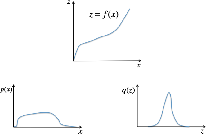
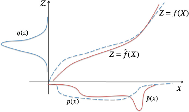
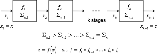
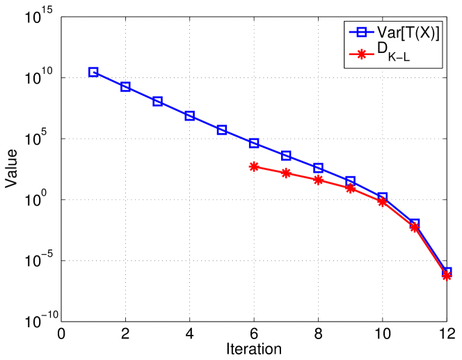
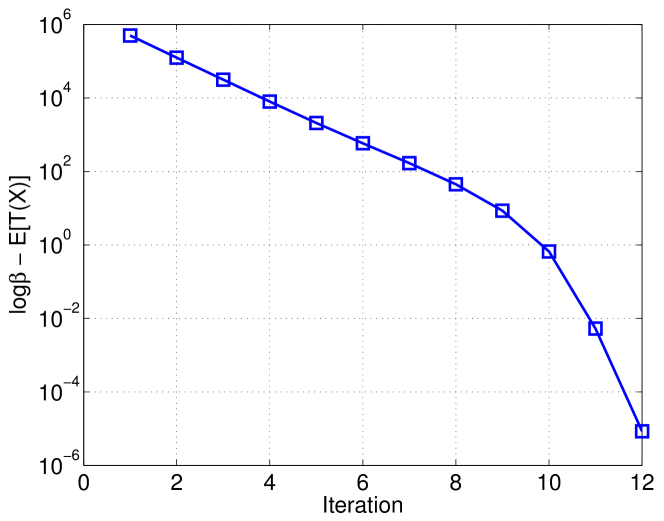
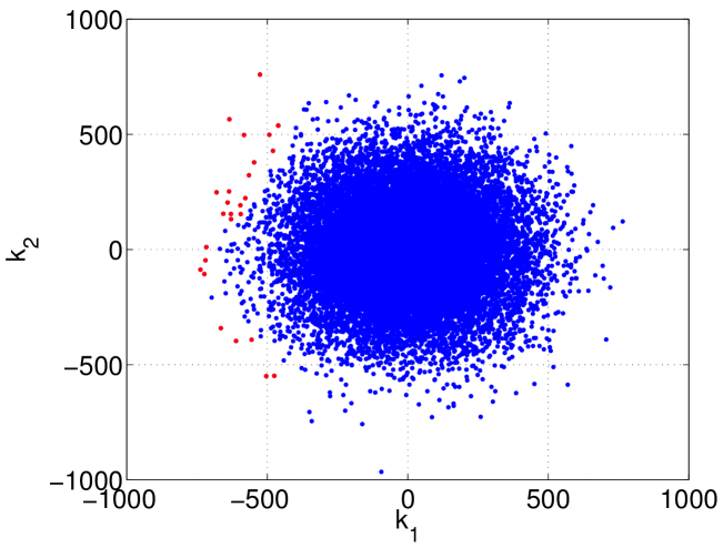
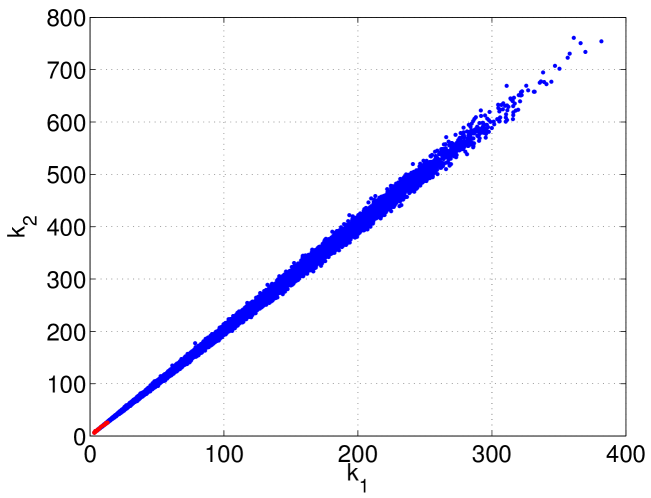
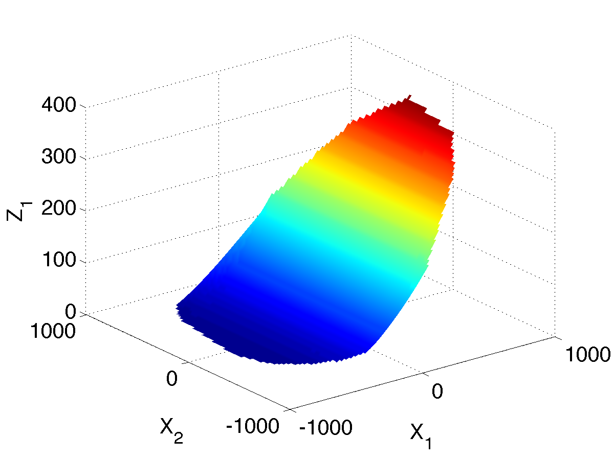
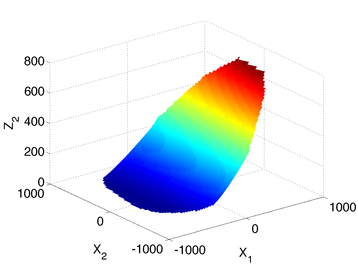
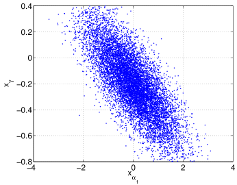
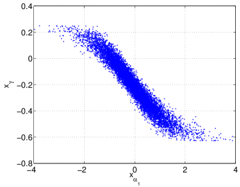
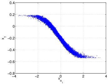
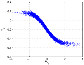
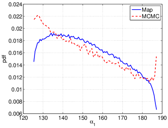
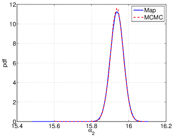
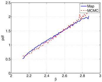
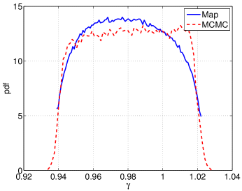
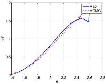
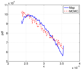
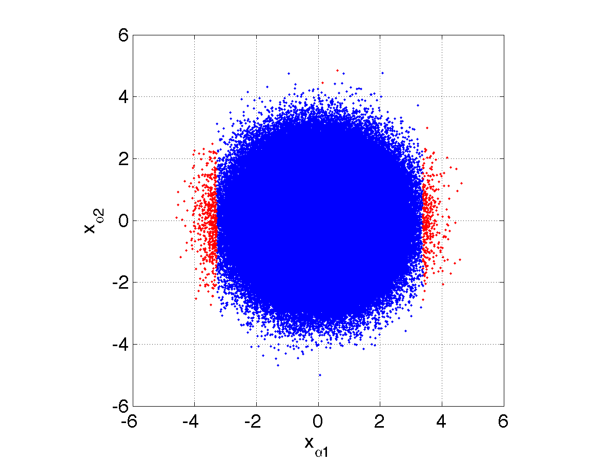
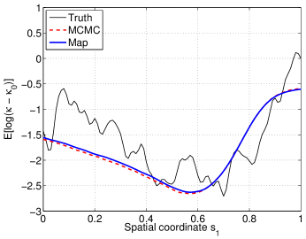
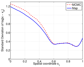
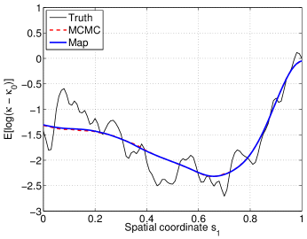
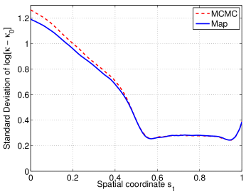
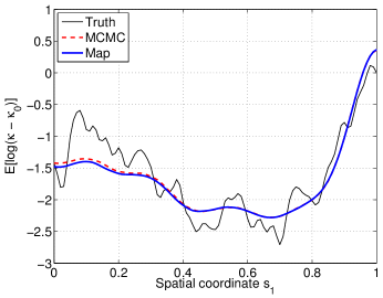
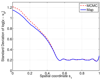
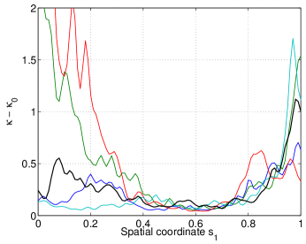
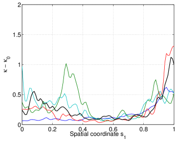
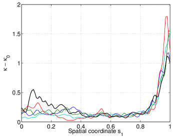
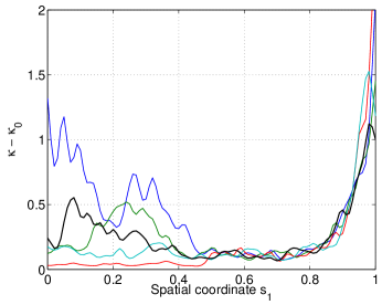
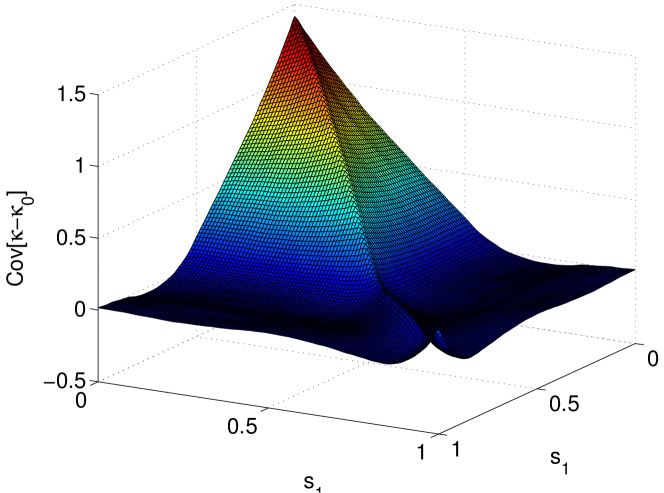
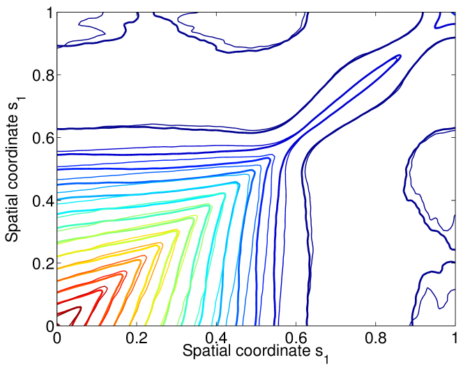
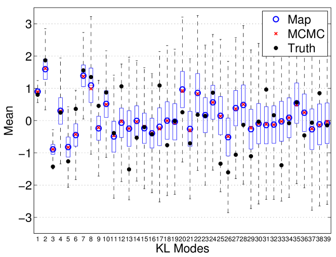
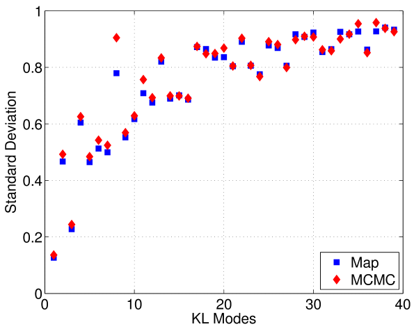
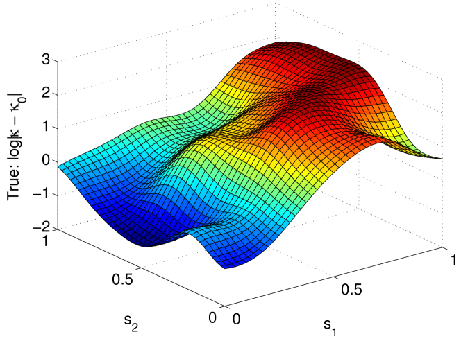
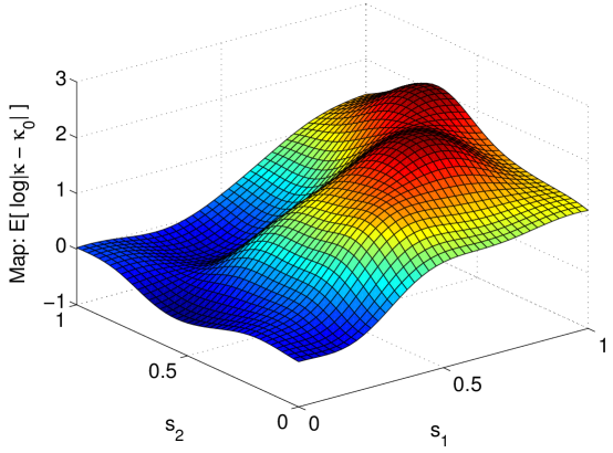
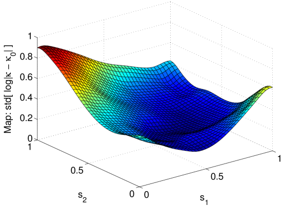
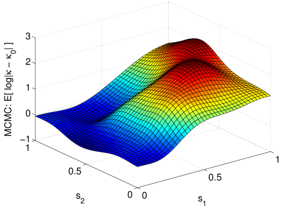
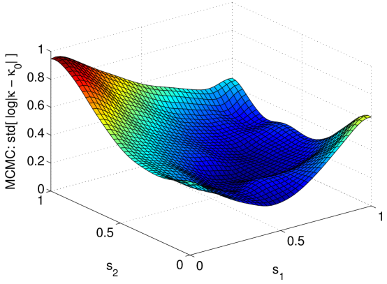
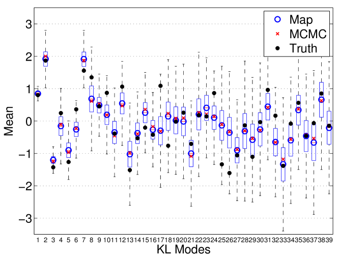
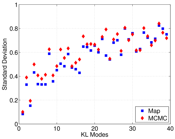
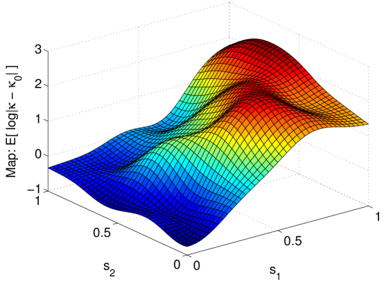
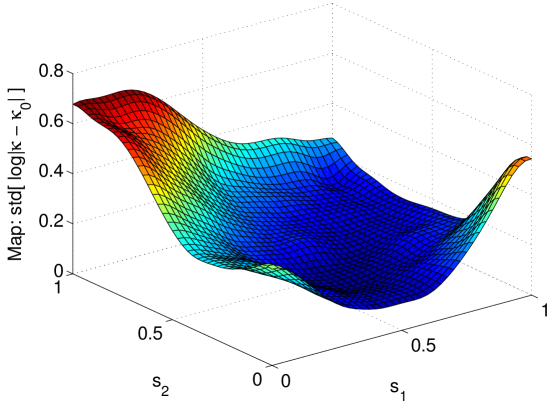
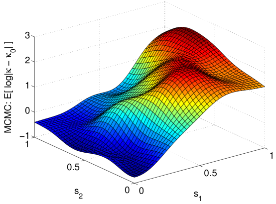
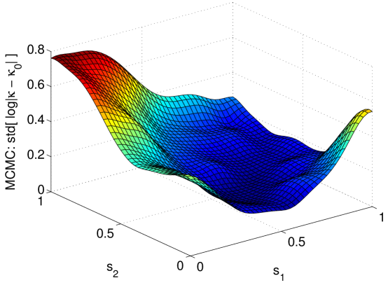
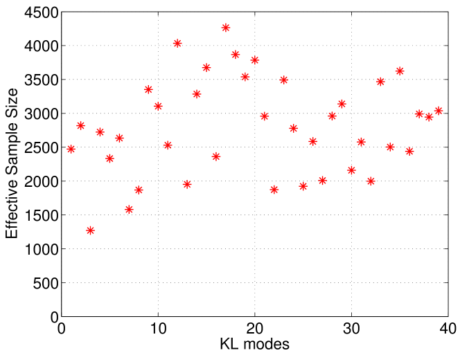
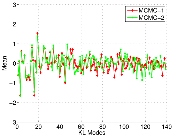
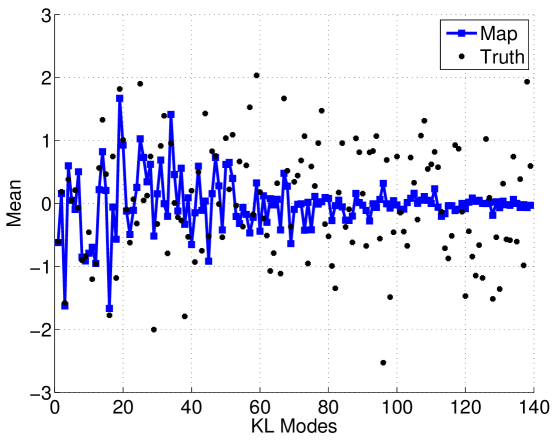
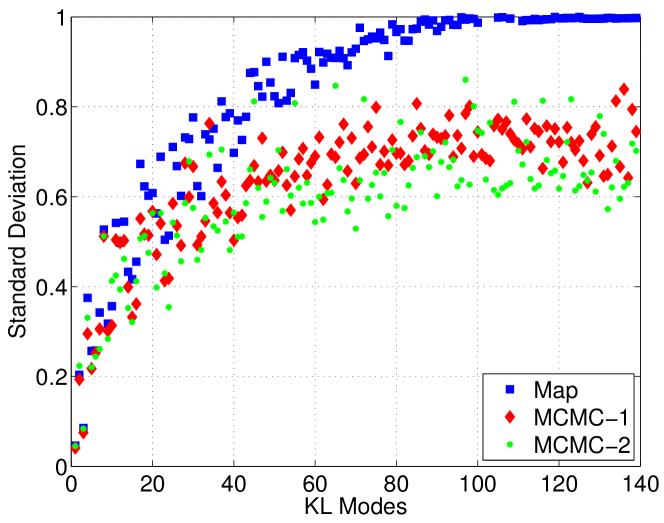
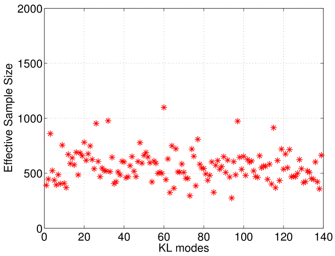
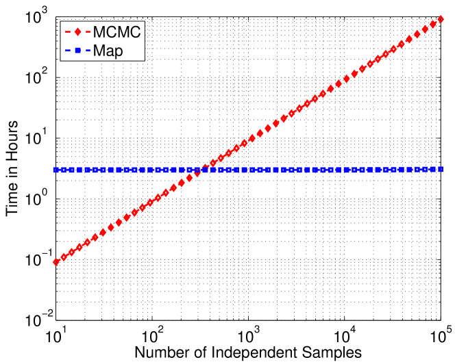
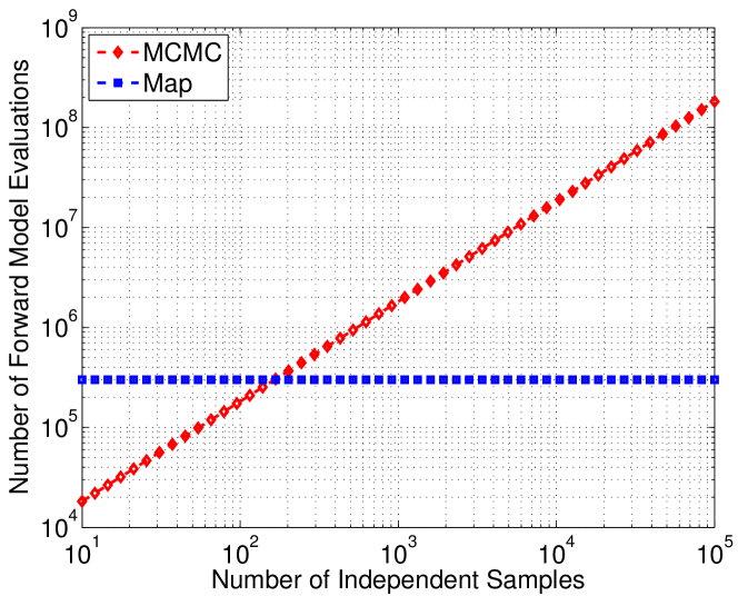
Appendix A Relation between variance and Kullback-Leibler divergence near convergence

When the variance of $T(X)$ is small, the Kullback Leibler-divergence from $p$ to $\tilde{p}$ is small as well. In this case, the relationship between these two quantities is asymptotically linear. To demonstrate this, we start from the KL divergence:

$$D_{\mathrm{KL}}\left(p||\tilde{p}\right)=\log\mathbb{E}\left[\exp\left(T\right)\right]-\mathbb{E}\left[T\right].$$ (60)

For small perturbations of $T$ around $T_{0}={\mathbb{E}}\left[T\right]$, we obtain

$$D_{\mathrm{KL}}\left(p||\tilde{p}\right) \approx \log\mathbb{E}\left[\exp{(T_{0})}\left(1+(T-T_{0})+\frac{1}{2}(T-T_{0})^{2}\right)\right]-\mathbb{E}\left[T_{0}\right]$$ (61)

$$= \log{\mathbb{E}\left[\left(1+(T-T_{0})+\frac{1}{2}(T-T_{0})^{2}\right)\right]}$$

$$= \log\left(1+\frac{1}{2}\operatorname{Var}\left[T\right]\right)$$

$$\approx \operatorname{Var}\left[T\right]/\,2$$

Appendix B Linear-Gaussian model

The special case of a linear forward model $h(x)=Ax$ with additive Gaussian noise $\varepsilon\sim N(0,\Sigma_{n})$ and a Gaussian prior $x\sim N(0,\Sigma_{P})$ admits a closed form solution, where the posterior is also Gaussian. Without loss of generality, we assume a prior mean of zero and write the posterior density $q$ as:

$$q(z) = \frac{1}{\beta}\exp{\left(-\frac{1}{2}\left(\|Az-d\|^{2}_{\Sigma_{n}}+\|z\|^{2}_{\Sigma_{P}}\right)\right)}$$ (62)

$$= \frac{1}{\beta}\exp{\left(-\frac{1}{2}\left(\|d\|^{2}_{\Sigma_{n}}+z^{T}\left(A^{T}{\Sigma_{n}^{-1}}A+{\Sigma_{P}^{-1}}\right)z+2d^{T}{\Sigma_{n}^{-1}}Az\right)\right)}$$

$$= \frac{1}{\beta}\exp{\left(-\frac{1}{2}\left(\|d\|^{2}_{\Sigma_{n}}+z^{T}\Sigma^{-1}z-2\mu^{T}\Sigma^{-1}z\right)\right)}$$

where $\mu$, $\Sigma$, and ${\beta}$ are the posterior mean, covariance, and evidence, respectively. Equating the second and third lines above, we obtain the following relations:

$$\Sigma = \left(A^{T}{\Sigma_{n}^{-1}}A+{\Sigma_{P}^{-1}}\right)^{-1}$$

$$\mu = \Sigma A^{T}{\Sigma_{n}^{-1}}d$$

$$\beta = \exp{\left(-\frac{1}{2}\left(\|d\|^{2}_{{\Sigma_{n}}}-\mu^{T}\Sigma^{-1}\mu^{T}\right)\right)}\sqrt{\left|\det{\Sigma}\right|}.$$ (63)

The map from the prior to the posterior is then given by

$$f(x)=z_{0}+Z_{1}x$$ (64)

where $z_{0}=\mu$ and the only constraint on $Z_{1}$ is that $\Sigma=Z_{1}\Sigma_{P}Z_{1}^{T}$.

This result is informative because it indicates that the matrix $Z_{1}$ is not uniquely determined. Indeed, if the prior covariance is the identity, then any orthonormal matrix $Q$ can result in a new map with $Z_{1}Q$ replacing $Z_{1}$.

Appendix C Nonlinear model with Gaussian prior and Gaussian additive noise

In this appendix we provide detailed expressions for derivatives with respect to optimization parameters in the case of a nonlinear forward model $h$, additive Gaussian observational error $\varepsilon\sim N(0,\Sigma_{n})$, and a Gaussian prior on the parameters $x$. For simplicity we let the prior have zero mean and identity covariance, $x\sim N(0,I)$. In particular, we obtain derivative expressions needed to solve the optimization problem when the map $f$ is represented with multivariate polynomials.

Let $p$ be the prior density, $q$ the posterior density, and $d$ the data. The problem setup is summarized as follows:

$$p(x) \propto \exp{\left(-\frac{1}{2}x^{T}x\right)}$$

$$d = h(z)+\varepsilon$$

$$q(z) = \frac{1}{\beta}\exp{\left(-\frac{1}{2}\left(\left\|h(z)-d\right\|_{\Sigma_{n}}^{2}+z^{T}z\right)\right)}$$

Using the map:

$$z=f(x)$$

we obtain the following $\tilde{p}$

$$\tilde{p}(x)=\frac{1}{\beta}\exp{\left(-\frac{1}{2}\left(\|h\left(f(x)\right)-d\|_{\Sigma_{n}}^{2}+f(x)^{T}f(x)-2\log{\left|\det D_{x}f\right|}\right)\right)}$$

where

$$\|h\left(f(x)\right)-d\|_{\Sigma_{n}}^{2}\equiv\left(h\left(f(x)\right)-d\right)^{T}\Sigma_{n}^{-1}\left(h\left(f(x)\right)-d\right)$$

and $\det D_{x}f$ is the determinant of the Jacobian of the map. Following (12), $T$ is given by

$$-2T(x)=\|h(f(x))-d\|^{2}_{\Sigma_{n}}+\|f(x)\|^{2}-2\log\left|\det D_{x}f\right|-\|x\|^{2}$$ (65)

Assume that the map is given by the polynomial chaos expansion (28)

$$f(x)=F^{T}\Psi(x).$$

We need to compute derivatives of $T(x;F)$ with respect to elements of the matrix $F$. Recall that $n$ is the dimension of the model parameter vector. Hence

$$z=f(x) = \left(\Psi(x)^{T}FI_{n}\right)^{T}=\left(I_{n}\otimes\Psi(x)^{T}\right)F(:)$$

$$\frac{\partial z}{\partial F}=\frac{\partial f(x)}{\partial F} = I_{n}\otimes\Psi^{T}$$ (66)

$$\frac{\partial h\left(f(x)\right)}{\partial F}=\frac{\partial h\left(F^{T}\Psi\right)}{\partial F} = \frac{\partial h(z)}{\partial z}\frac{\partial z}{\partial F}=\frac{\partial h}{\partial z}\left(I_{n}\otimes\Psi^{T}\right)$$ (67)

and

$$D_{x}f\equiv\frac{\partial f}{\partial x} = F^{T}\frac{\partial\Psi}{\partial x}$$

$$\frac{\partial\left(\log\left|\det D_{x}f\right|\right)}{\partial F} = \operatorname{trace}\left(\left[D_{x}f\right]^{-1}\frac{\partial}{\partial F_{ij}}\left[D_{x}f\right]\right)$$ (68)

$$= \left[\frac{\partial\Psi}{\partial x}\left(F^{T}\frac{\partial\Psi}{\partial x}\right)^{-1}\right](:)$$

where the notation $\left[A\right](:)$ signifies a rearrangement of the elements of the rectangular matrix $A$ into a single column vector. Returning to (65) above, we obtain the following expression for the first derivatives of $T$ evaluated at $x$:

$$\frac{\partial T(x;F)}{\partial F}=-\left(\frac{\partial h\left(f(x)\right)}{\partial F}\right)^{T}\Sigma_{n}^{-1}\left(h\left(f\left(x\right)\right)-d\right)-\left(\frac{\partial f(x)}{\partial F}\right)^{T}f(x)+\left[\frac{\partial\Psi}{\partial x}\left(F^{T}\frac{\partial\Psi}{\partial x}\right)^{-1}\right](:)$$

Using (66) and (67)

$$\frac{\partial T(x;F)}{\partial F} = -\left(\frac{\partial h(z)}{\partial z}^{T}\Sigma_{n}^{-1}\left(h\left(f\left(x\right)\right)-d\right)+f(x)\right)\otimes\Psi$$ (69)

$$+\left[\frac{\partial\Psi}{\partial x}\left(F^{T}\frac{\partial\Psi}{\partial x}\right)^{-1}\right](:),$$

where derivatives with respect to $z$ are evaluated at $z=f(x)$.

To evaluate the second derivatives needed for Newton’s method, one needs to compute the second derivative of the logarithm of the Jacobian determinant:

$$\frac{\partial\log|\det D_{x}f|}{\partial F_{ij}} = \left(\frac{\partial\Psi}{\partial x}(i,:)\left(D_{x}f\right)^{-1}\right)[j]$$

$$\frac{\partial\log{|\det D_{x}f|}}{\partial F_{ij}} = \frac{\partial\Psi}{\partial x}(i,:)\left(D_{x}f\right)^{-1}e_{j}$$

$$\frac{\partial^{2}\log{|\det D_{x}f|}}{\partial F_{ij}\partial F_{mn}} = -\frac{d\Psi}{dx}(i,:)\left(D_{x}f\right)^{-1}\left(e_{n}\frac{\partial\Psi}{\partial x}(m,:)\right)\left(D_{x}f\right)^{-1}e_{j}$$

$$\frac{\partial^{2}\log{|\det D_{x}f|}}{\partial F_{ij}\partial F_{mn}} = -\left(\frac{\partial\Psi}{\partial x}(i,:)\left(D_{x}f\right)^{-1}\right)e_{n}\left(\frac{\partial\Psi}{\partial x}(m,:)\left(D_{x}f\right)^{-1}\right)e_{j}$$

where $e_{j}$ is a vector of all zeros except for a 1 in the $j$th location. It is clear that the only expensive quantity to be computed is the matrix

$$\mathcal{M}=\frac{\partial\Psi}{\partial x}\left(D_{x}f\right)^{-1}$$

$$\frac{\partial^{2}\log|\det D_{x}f|}{\partial F_{ij}\partial F_{mn}}=-\mathcal{M}(i,n)\mathcal{M}(m,j)$$

$$\frac{\partial^{2}T}{\partial F_{ij}\partial F_{mn}} = -\left(\frac{\partial h(f(x))}{\partial F_{ij}}\right)^{T}\Sigma_{n}^{-1}\frac{\partial h(f(x))}{\partial F_{mn}}-\left(\frac{\partial^{2}h(f(x))}{\partial F_{ij}\partial F_{mn}}\right)^{T}\Sigma_{n}^{-1}(h(f(x))-d)$$ (70)

$$-\left(\frac{\partial f(x)}{\partial F_{ij}}\right)^{T}\frac{\partial f(x)}{\partial F_{mn}}-\mathcal{M}(i,n)\mathcal{M}(m,j).$$

Notice that storage of the object ${\partial^{2}h(f(x))}/{\partial F\partial F}$ requires special care in implementation, since it is the second derivative of a vector-valued function with respect to a vector. We find that it is best stored as a third-order tensor of dimension $m\times\ell\times\ell$, where $m$ is the number of observations and $\ell$ is the number of optimization variables. Alternatively, one could instead retain only the second derivative of the term $\|h(z)-d\|_{\Sigma_{n}}^{2}$ with respect to $F$, which can be stored in standard matrix format. For example, consider the special case in which the forward model $h$ is approximated using the polynomial chaos expansion

$$h(z)=C^{T}\Psi_{h}(z)$$

where $C$ is the output matrix and has $m$ columns. The second derivative of $\|h(z)-d\|_{\Sigma_{n}}^{2}$ with respect to $F$ is computed as follows:

$$\left(\frac{\partial h(f(x))}{\partial F}\right)^{T}\Sigma_{n}^{-1}\left(\frac{\partial h(f(x))}{\partial F}\right) + \sum\limits_{j=1}^{m}\sum\limits_{i=1}^{m}\left(\frac{\partial^{2}h_{i}(f(x))}{\partial F\partial F}\right)^{T}\left[\Sigma_{n}^{-1}\right](i,j)(h_{j}(f(x))-d_{j})$$

$$= \left(C^{T}\frac{\partial\Psi_{h}(z)}{\partial z}\frac{\partial f(x)}{\partial F}\right)^{T}\Sigma_{n}^{-1}\left(C^{T}\frac{\partial\Psi_{h}(z)}{\partial z}\frac{\partial f(x)}{\partial F}\right)$$

$$+\sum\limits_{j=1}^{n}\left(C^{T}\frac{\partial^{2}\Psi_{h}(z)}{\partial z\partial z_{j}}\frac{\partial f(x)}{\partial F}\right)^{T}\Sigma_{n}^{-1}(h(f(x))-d)\left(\frac{\partial f_{j}(x)}{\partial F}\right).$$

Putting everything together we arrive at the following expression for ${\partial^{2}T(x)}/{\partial F\partial F}$:

$$\frac{\partial^{2}T}{\partial F\partial F} = -\left(\left(\frac{\partial\Psi_{h}(f(x))}{\partial f(x)}\right)^{T}C\Sigma_{n}^{-1}C^{T}\frac{\partial\Psi_{h}(f(x))}{\partial f(x)}\right)\otimes\Psi\Psi^{T}$$ (71)

$$-\left(\sum\limits_{j=1}^{n}\left(\frac{\partial^{2}\Psi_{h}(f(x))}{\partial f(x)\partial f_{j}(x)}\right)^{T}C\Sigma_{n}^{-1}(C^{T}\Psi_{h}(f(x))-d)e_{j}^{T}+I_{n}\right)\otimes\Psi\Psi^{T}$$

$$-{\mathcal{M}}^{T}\otimes{\mathcal{M}}.$$

References

- Stuart [2010] A. M. Stuart, Inverse problems: a Bayesian perspective, Acta Numerica 19 (2010) 451–559.
- Gelman et al. [2003] A. Gelman, J. B. Carlin, H. S. Stern, D. B. Rubin, Bayesian Data Analysis, Chapman and Hall/CRC, 2nd edition, 2003.
- Kaipio and Somersalo [2004] J. Kaipio, E. Somersalo, Statistical and Computational Inverse Problems, Springer, 2004.
- Sivia and Skilling [2006] D. S. Sivia, J. Skilling, Data Analysis: A Bayesian Tutorial, Oxford Science Publications, 2nd edition, 2006.
- Bernardo and Smith [1994] J. M. Bernardo, A. F. M. Smith, Bayesian Theory, Wiley, 1994.
- Metropolis et al. [1953] N. Metropolis, A. W. Rosenbluth, M. N. Rosenbluth, A. H. Teller, E. Teller, Equation of state calculations by fast computing machines, The Journal of Chemical Physics 21 (1953) 1087–1092.
- Hastings [1970] W. K. Hastings, Monte Carlo sampling methods using Markov chains and their applications, Biometrika 57 (1970) 97–109.
- Gilks et al. [1996] W. Gilks, W. Gilks, S. Richardson, D. Spiegelhalter, Markov Chain Monte Carlo in Practice, Chapman & Hall, 1996.
- Robert and Casella [2004] C. P. Robert, G. Casella, Monte Carlo Statistical Methods, Springer-Verlag, 2nd edition, 2004.
- Liu [2008] J. S. Liu, Monte Carlo Strategies in Scientific Computing, Springer, 2008.
- Haario et al. [2006] H. Haario, M. Laine, A. Mira, E. Saksman, DRAM: Efficient adaptive MCMC, Statistics and Computing 16 (2006) 339–354.
- Roberts and Rosenthal [2009] G. O. Roberts, J. S. Rosenthal, Examples of adaptive MCMC, Journal of Computational and Graphical Statistics 18 (2009) 349–367.
- Stramer and Tweedie [1999] O. Stramer, R. Tweedie, Langevin-type models II: Self-targeting candidates for MCMC algorithms, Methodology and Computing in Applied Probability 1 (1999) 307–328.
- Apte et al. [2007] A. Apte, M. Hairer, A. Stuart, J. Voss, Sampling the posterior: an approach to non-Gaussian data assimilation, Physica D: Nonlinear Phenomena 230 (2007) 50–64.
- Girolami and Calderhead [2011] M. Girolami, B. Calderhead, Riemann manifold Langevin and Hamiltonian Monte Carlo methods, Journal of the Royal Statistical Society: Series B (Statistical Methodology) 73 (2011) 123–214.
- Martin et al. [2012] J. Martin, L. Wilcox, C. Burstedde, O. Ghattas, A stochastic Newton MCMC method for large-scale statistical inverse problems, SIAM Journal on Scientific Computing (2012). To appear.
- Neal [2011] R. M. Neal, MCMC using Hamiltonian dynamics, in: S. Brooks, A. Gelman, G. Jones, X. Meng (Eds.), Handbook of Markov Chain Monte Carlo, Chapman and Hall/CRC Press, 2011, pp. 113–162.
- Higdon et al. [2002] D. Higdon, H. Lee, Z. Bi, A Bayesian approach to characterizing uncertainty in inverse problems using coarse and fine-scale information, IEEE Transactions on Signal Processing 50 (2002) 389–399.
- Vrugt et al. [2009] J. A. Vrugt, C. J. F. ter Braak, C. G. H. Diks, B. A. Robinson, J. M. Hyman, D. Higdon, Accelerating Markov chain Monte Carlo simulation by differential evolution with self-adaptive randomized subspace sampling, International Journal of Nonlinear Sciences and Numerical Simulation 10 (2009) 273–290.
- Craiu et al. [2009] R. V. Craiu, J. Rosenthal, C. Yang, Learn from thy neighbor: Parallel-chain and regional adaptive MCMC, Journal of the American Statistical Association 104 (2009) 1454–1466.
- Christen and Fox [2005] J. A. Christen, C. Fox, Markov chain Monte Carlo using an approximation, Journal of Computational and Graphical Statistics 14 (2005) 795–810.
- Efendiev et al. [2006] Y. Efendiev, T. Y. Hou, W. Luo, Preconditioning Markov chain Monte Carlo simulations using coarse-scale models, SIAM Journal on Scientific Computing 28 (2006) 776–803.
- Marzouk et al. [2007] Y. M. Marzouk, H. N. Najm, L. A. Rahn, Stochastic spectral methods for efficient Bayesian solution of inverse problems, Journal of Computational Physics 224 (2007) 560–586.
- Marzouk and Najm [2009] Y. M. Marzouk, H. N. Najm, Dimensionality reduction and polynomial chaos acceleration of Bayesian inference in inverse problems, Journal of Computational Physics 228 (2009) 1862–1902.
- Lieberman et al. [2010] C. Lieberman, K. Willcox, O. Ghattas, Parameter and state model reduction for large-scale statistical inverse problems, SIAM Journal on Scientific Computing 32 (2010) 2485–2496.
- Frangos et al. [2010] M. Frangos, Y. Marzouk, K. Willcox, B. van Bloemen Waanders, Surrogate and reduced-order modeling: a comparison of approaches for large-scale statistical inverse problems, in: L. Biegler, G. Biros, O. Ghattas, M. Heinkenschloss, D. Keyes, B. Mallick, Y. Marzouk, L. Tenorio, B. van Bloemen Waanders, , K. Willcox (Eds.), Computational Methods for Large-Scale Inverse Problems and Quantification of Uncertainty, Wiley, 2010, pp. 123–149.
- Wang and Zabaras [2005] J. Wang, N. Zabaras, Using Bayesian statistics in the estimation of heat source in radiation, International Journal of Heat and Mass Transfer 48 (2005) 15–29.
- Gelman and Shirley [2011] A. Gelman, K. Shirley, Inference from simulations and monitoring convergence, in: S. Brooks, A. Gelman, G. Jones, X. Meng (Eds.), Handbook of Markov Chain Monte Carlo, Chapman and Hall/CRC Press, 2011, pp. 163–174.
- Ghanem and Spanos [2003] R. Ghanem, P. Spanos, Stochastic Finite Elements: a Spectral Approach, Dover Publications, 2003.
- LeMaître and Knio [2010] O. P. LeMaître, O. M. Knio, Spectral Methods for Uncertainty Quantification: with Applications to Computational Fluid Dynamics, Springer, 2010.
- Xiu [2010] D. Xiu, Numerical Methods for Stochastic Computations: A Spectral Method Approach, Princeton University Press, 2010.
- Doucet et al. [2001] A. Doucet, N. Freitas, N. Gordon, Sequential Monte Carlo Methods in Practice, Springer, 2001.
- McCann [1995] R. J. McCann, Existence and uniqueness of monotone measure-preserving maps, Duke Mathematical Journal 80 (1995) 309–323.
- Xiu and Karniadakis [2002] D. Xiu, G. Karniadakis, The Wiener-Askey polynomial chaos for stochastic differential equations, SIAM Journal on Scientific Computing 24 (2002) 619–644.
- Kass and Raftery [1995] R. E. Kass, A. E. Raftery, Bayes factors, Journal of the American Statistical Association 90 (1995) 773–795.
- Jaakkola and Jordan [2000] T. Jaakkola, M. Jordan, Bayesian parameter estimation via variational methods, Statistics and Computing 10 (2000) 25–37.
- Chorin and Tu [2009] A. J. Chorin, X. Tu, Implicit sampling for particle filters, Proceedings of the National Academy of Sciences USA 106 (2009) 17249–17254.
- Chorin et al. [2010] A. Chorin, M. Morzfeld, X. Tu, Implicit particle filters for data assimilation, Communications in Applied Mathematics and Computational Science 5 (2010) 221–240.
- Reich [2011] S. Reich, A dynamical systems framework for intermittent data assimilation, BIT Numerical Mathematics 51 (2011) 235–249.
- Tarantola [2005] A. Tarantola, Inverse problem theory and methods for model parameter estimation, Society for Industrial and Applied Mathematics, 2005.
- McShane [1937] E. J. McShane, Jensen’s inequality, Bulletin of the American Mathematical Society 43 (1937) 521–527.
- Brenier [1991] Y. Brenier, Polar factorization and monotone rearrangement of vector-valued functions, Communications on Pure and Applied Mathematics 44 (1991) 375–417.
- Caffarelli [1992] L. A. Caffarelli, The regularity of mappings with a convex potential, Journal of the American Mathematical Society 5 (1992) 99–104.
- Gangbo and McCann [1996] W. Gangbo, R. J. McCann, The geometry of optimal transportation, Acta Mathematica 177 (1996) 113–161.
- Villani [2009] C. Villani, Optimal Transport: Old and New, Springer, 2009.
- Rosenblatt [1952] M. Rosenblatt, Remarks on a multivariate transformation, The Annals of Mathematical Statistics 23 (1952) 470–472.
- Knothe [1957] H. Knothe, Contributions to the theory of convex bodies, Michigan Mathematical Journal 4 (1957) 39–52.
- Carlier et al. [2010] G. Carlier, A. Galichon, F. Santambrogio, From Knothe’s transport to Brenier’s map and a continuation method for optimal transport, SIAM Journal on Mathematical Analysis 41 (2010).
- Nemirovski et al. [2009] A. Nemirovski, A. Juditsky, G. Lan, A. Shapiro, Robust stochastic approximation approach to stochastic programming, SIAM Journal on Optimization 19 (2009) 1574–1609.
- Wiener [1938] N. Wiener, The homogeneous chaos, American Journal of Mathematics 60 (1938) 897–936.
- Soize and Ghanem [2004] C. Soize, R. Ghanem, Physical systems with random uncertainties: Chaos representations with arbitrary probability measure, SIAM Journal on Scientific Computing 26 (2004) 395–410.
- Rupert and Miller [2007] C. Rupert, C. Miller, An analysis of polynomial chaos approximations for modeling single-fluid-phase flow in porous medium systems, Journal of Computational Physics 226 (2007) 2175–2205.
- Gardner et al. [2000] T. S. Gardner, C. R. Cantor, J. J. Collins, Construction of a genetic toggle switch in escherichia coli., Nature 403 (2000) 339–342.
- Marzouk and Xiu [2009] Y. M. Marzouk, D. Xiu, A stochastic collocation approach to Bayesian inference in inverse problems, Communications in Computational Physics 6 (2009) 826–847.
- Dashti and Stuart [2012] M. Dashti, A. Stuart, Uncertainty quantification and weak approximation of elliptic inverse, SIAM Journal on Numerical Analysis (2012). To appear.
- Rasmussen and Williams [2006] C. E. Rasmussen, C. K. I. Williams, Gaussian processes for machine learning, MIT Press, 2006.
- Papaspiliopoulos et al. [2012] O. Papaspiliopoulos, Y. Pokern, G. O. Roberts, A. Stuart, Nonparametric estimation of diffusions: a differential equations approach, Biometrika (2012). To appear.
- Moselhy and Marzouk [2011] T. A. Moselhy, Y. M. Marzouk, An adaptive iterative method for high-dimensional stochastic PDEs, 2011. Preprint.
- Cotter et al. [2012] S. Cotter, G. Roberts, A. Stuart, D. White, MCMC methods for functions: Modifying old algorithms to make them faster (2012). ArXiv:1202.0709.
- Wan and Karniadakis [2005] X. Wan, G. E. Karniadakis, An adaptive multi-element generalized polynomial chaos method for stochastic differential equations, Journal of Computational Physics 209 (2005) 617–642.