Transmission in waveguides with compositional and structural disorder: experimental effects of disorder cross-correlations

Abstract

We analyse the single-mode transmission of microwaves in a guide with internal random structure. The waveguide contains scatterers characterised by random heights and positions, corresponding to compositional and structural disorder. We measure the effects of cross-correlations between two kinds of disorder, showing how they enhance or attenuate the experimentally found transmission gaps generated by long-range self-correlations. The results agree with the theoretical predictions obtained for the aperiodic Kronig-Penney model and prove that self- and cross-correlations have relevant effects also in finite disordered samples of small size.

Keywords: Correlated disorder, anomalous localisation, microwave guide, Kronig-Penney model, cross-correlation

1 Introduction

At the end of the 1990s it was realised that, contrary to previously held beliefs, effective localisation-delocalisation transitions can take place in one-dimensional (1D) and quasi-1D random models, provided that disorder is endowed with specific long-range correlations [1, 2, 3, 4]. In particular, the study of 1D models with correlated random potentials was greatly spurred by the seminal paper of Izrailev and Krokhin [3, 4], who derived an analytical formula for the localisation length in one-dimensional models with weak correlated disorder. The discovery triggered an intense research activity in the field of low-dimensional models, which are now understood to possess a much richer behaviour than once thought (for a review, see [5]).

The theoretical predictions about the existence of delocalised states in 1D or quasi-1D models with correlated disorder [6, 1, 2, 3, 4] soon found experimental confirmations in semiconductor superlattices [7] and microwave waveguides [8, 9]. Since these early works, 1D models with correlated disorder have found applications in an increasing number of physical fields, including Bose-Einstein condensates [10, 11, 12], bilayered media [13], structures with corrugated surfaces [14, 15], and DNA modelling [16, 17].

In most of these works, the system under consideration has a single self-correlated random potential. Recently, however, some theoretical studies have begun to explore more complex models, characterised by the simultaneous presence of two kinds of disorder. For instance, in [13] the authors considered the transport properties of generic bilayered structures formed by infinite arrays of alternating slabs of two different kinds. Since slabs of both types can have random widths, each structure is characterised not by one but by two random sequences which, in addition to self-correlations, can exhibit cross-correlations. Another model exhibiting two types of disorder is the aperiodic Kronig-Penney model with both compositional and structural disorder [18, 19, 20]. For this model, it was possible to work out a perturbative expression for the localisation length of the quantum states valid for weak disorder with any kind of self- and cross-correlations [18]. The theoretical results for the localisation length of electronic states showed that the interplay of structural and compositional disorder could enhance the delocalisation-localisation transition created by long-range self-correlations of each type of disorder. It was also shown that cross-correlations could affect the transmission properties of a long random sample, increasing or decreasing the transmittivity in the opaque windows corresponding to the localised states.

These findings posed the question of whether these effects could be experimentally observed in appropriately designed random microwave waveguides. In fact, the structure of the electronic states in a Kronig-Penney model and the transmission of the waveguide with point-like scatterers are closely related problems because the Schrödinger equation for the former model has the same form of the Helmholtz equation for the latter. Because of this analogy, the theoretical results originally obtained in [21] for a Kronig-Penney model with purely structural disorder immediately found experimental applications in the analysis of the transmission properties of single-mode waveguides [8, 9, 22]. It was therefore natural to ask whether the theoretical predictions concerning the effects of cross-correlations in the aperiodic Kronig-Penney model could find an experimental confirmation in suitable random waveguides. The main goal of this paper is to analyse this question, which we answer in the affirmative.

We considered microwave transmission of the first mode in a Q1D waveguide open on both ends and with no intermode coupling. The waveguide contained scatterers constituted by brass bars situated at random positions (structural disorder) and having random heights (compositional disorder). We found that cross-correlations of the random spacings with the heights have a sizable effect on the transmission properties of the waveguide in agreement with theoretical predictions. This is a remarkable finding, because the theoretical results for the localisation length are derived for an infinite array with weak disorder, whereas the experimental measures were obtained using a setup of finite size, with a modest number of scatterers (40 bars) and relatively strong disorder. The experimental data therefore show that the effect of disorder correlation is robust and is not washed away by other features of the apparatus (such as absorption) which are neglected in the simplified theoretical description.

This paper is organised as follows. In section 2 we outline the theoretical framework. In section 3 we describe the setup. Our experimental findings are presented in section 4. We summarise our findings and expose our conclusions in section 5.

2 Theoretical considerations

We analyse the transmission of microwaves in a rectangular waveguide with internal scatterers, constituted by brass bars situated at random positions and having random heights. If one assumes that the bars can be assimilated to point-like scatterers and represented as delta-barriers, the propagation of a single mode in the waveguide can be described using a Helmholtz equation which has the same mathematical form of the Schrödinger equation for the aperiodic Kronig-Penney model with delta-barriers [8, 9]

$$-\psi^{\prime\prime}(x)+\left[\sum_{n=-\infty}^{\infty}(U+u_{n})\delta(x-n-a_{n})\right]\psi(x)=E\psi(x).$$ (1)

For the sake of simplicity, here and in the rest of the paper we use energy units such that $\hbar^{2}/2m=1$ and set the lattice step as unit length.

The model (1), as the associated waveguide, has a twofold randomness: on the one hand, the positions of the delta-barriers present random shifts $a_{n}$ with respect to the lattice sites (structural disorder). On the other hand, compositional disorder is introduced via the fluctuations $u_{n}$ of the barrier strengths around the mean value $U$. The statistical properties of model (1) are defined by assuming that the random variables $u_{n}$ and $a_{n}$ have vanishing averages and known binary correlators. In the case of weak-disorder no further specification of the statistical features of the model is required. The weak-disorder case is identified by the conditions [18, 19, 20]

$$\begin{array}[]{cccc}\langle u_{n}^{2}\rangle\ll U^{2},&\langle\Delta_{n}^{2}\rangle E\ll 1,&\mbox{ and }&\langle\Delta_{n}^{2}\rangle U\ll 1,\end{array}$$

with $\Delta_{n}=a_{n+1}-a_{n}$ representing the relative displacement of two contiguous barriers.

If disorder is weak, one can obtain an analytical expression for the localisation length $l_{loc}$ of the electronic states $\psi$ of the model (1) [18, 19, 20]. Following the Hamiltonian map approach, one can show that, within the second-order approximation, the electronic states have an inverse localisation length equal to

$$\begin{array}[]{ccl}l_{\mathrm{loc}}^{-1}&=&\displaystyle\frac{1}{8\sin^{2}\kappa}\left[\frac{\sin^{2}k}{k^{2}}\langle u_{n}^{2}\rangle W_{1}(\kappa)+U^{2}\langle\Delta_{n}^{2}\rangle W_{2}(\kappa)\right.\\ &-&\displaystyle\left.2U\frac{\sin(k)}{k}\langle u_{n}\Delta_{n}\rangle\cos\left(\kappa\right)W_{3}(\kappa)\right].\end{array}$$ (2)

In (2) the symbols $k$ and $\kappa$ represent respectively the propagation wavevector within the wells $k=\sqrt{E}$ and the Bloch wavevector $\kappa$ of the quantum particle. The two quantities are linked by the condition

$$\cos\kappa=\cos k+\frac{U}{2k}\sin k,$$ (3)

which defines the band structure of the Kronig-Penney model (1) in the absence of disorder. The functions $W_{i}(\kappa)$ in (2), on the other hand, are the Fourier transforms of the normalised binary correlators of the random variables $u_{n}$ and $\Delta_{n}$, i.e.,

$$\begin{array}[]{ccl}W_{1}\left(\kappa\right)&=&\displaystyle 1+2\sum_{l=1}^{\infty}\frac{\langle u_{n}u_{n+l}\rangle}{\langle u_{n}^{2}\rangle}\cos(2\kappa l)\\ W_{2}\left(\kappa\right)&=&\displaystyle 1+2\sum_{l=1}^{\infty}\frac{\langle\Delta_{n}\Delta_{n+l}\rangle}{\langle\Delta_{n}^{2}\rangle}\cos(2\kappa l)\\ W_{3}\left(\kappa\right)&=&\displaystyle 1+2\sum_{l=1}^{\infty}\frac{\langle u_{n}\Delta_{n+l}\rangle}{\langle u_{n}\Delta_{n}\rangle}\cos(2\kappa l).\\ \end{array}$$ (4)

Equation (2) shows that the localisation length diverges (within the second-order approximation) in any given energy interval with vanishing power spectra (4). Therefore an effective localisation-delocalisation transition can occur in the 1D Kronig-Penney model (1) provided that the disorder exhibits the specific long-range correlations which make the power spectra (4) vanish over a continuous energy range.

In order to obtain a specific localisation-delocalisation transition with pre-assigned mobility edges, one must know how to construct two random sequences $\{u_{n}\}$ and $\{\Delta_{n}\}$ such that the corresponding power spectra (4) vanish in pre-defined energy intervals. A solution to this problem was presented in [20]; the basic idea is to generate two independent white-noise sequences which, after having been cross-correlated, can be endowed with the appropriate self-correlations with a filtering process. More precisely, one starts with two sequences $\{X_{n}^{(1)}\}$ and $\{X_{n}^{(2)}\}$ of independent identically distributed random variables. Two cross-correlated white noises can then be obtained by using the transformation

$$\begin{array}[]{ccl}Y_{n}^{(1)}&=&X_{n}^{(1)}\cos\eta+X_{n}^{(2)}\sin\eta\\ Y_{n}^{(2)}&=&X_{n}^{(1)}\sin\eta+X_{n}^{(2)}\cos\eta,\\ \end{array}$$

where $\eta$ determines the degree of cross-correlation of the $Y$ variables. The values of $\eta$ lie in the interval $[-\pi/4,\pi/4]$ with $\eta=\pm\pi/4$ corresponding to the extreme cases of total positive and negative cross-correlation, while for $\eta=0$ the cross-correlations vanish. The cross-correlated white noises $Y_{n}^{(1)}$ and $Y_{n}^{(2)}$ can then acquire the required self-correlations by means of the convolution products

$$\begin{array}[]{ccl}u_{n}&=&\displaystyle\sum_{l=-\infty}^{\infty}\alpha_{l}Y_{n-l}^{(1)}\\ \Delta_{n}&=&\displaystyle\sum_{l=-\infty}^{\infty}\beta_{l}Y_{n-l}^{(2)}\\ \end{array}$$ (5)

in which the coefficients $\alpha_{n}$ and $\beta_{n}$ are derived by the pre-defined power spectra $W_{1}$ and $W_{2}$ via the equations

$$\begin{array}[]{ccl}\alpha_{n}&=&\displaystyle\frac{2}{\pi}\int_{0}^{\pi/2}\sqrt{\langle u_{l}^{2}\rangle W_{1}(x)}\cos\left(2nx\right)\mathrm{d}x\\ \beta_{n}&=&\displaystyle\frac{2}{\pi}\int_{0}^{\pi/2}\sqrt{\langle\Delta_{l}^{2}\rangle W_{2}(x)}\cos\left(2nx\right)\mathrm{d}x.\\ \end{array}$$ (6)

After substituting the random variables defined by (5) and (6) in (2), the inverse localisation length takes the form

$$\begin{array}[]{ccl}l_{\mathrm{loc}}^{-1}&=&\displaystyle\frac{1}{8\sin^{2}\kappa}\left[\left(\frac{\sin k}{k}\right)^{2}\langle u_{n}^{2}\rangle W_{1}(\kappa)+U^{2}\langle\Delta_{n}^{2}\rangle W_{2}(\kappa)\right.\\ &-&\displaystyle\left.2\left|\frac{\sin k}{k}\right|U\sqrt{\langle u_{n}^{2}\rangle\langle\Delta_{n}^{2}\rangle W_{1}(\kappa)W_{2}(\kappa)}\;\cos\kappa\sin\left(2\eta\right)\right].\end{array}$$ (7)

As a simple example of delocalisation transition produced by self-correlations and modulated by cross-correlations, one can consider the case in which both structural and compositional disorder have a power spectrum of the form

$$W_{1}(\kappa)=W_{2}(\kappa)=\left\{\begin{array}[]{ccl}\displaystyle\frac{\pi}{2a\left(\kappa_{2}-\kappa_{1}\right)}&\mbox{ if }&\kappa\in\left[\kappa_{1},\kappa_{2}\right]\\ 0&\mbox{ if }&\kappa\in\left[0,\kappa_{1}\right]\cup\left[\kappa_{2},\frac{\pi}{2}\right]\\ \end{array}\right.$$ (8)

with $0<\kappa_{1}<\kappa_{2}<\pi/2$. Note that it is enough to consider the $[0,\pi/2]$ interval in the previous definition because the power spectra (4) are even functions of period $\pi$. The binary self-correlators corresponding to the power spectra (8) decrease with a power law

$$\frac{\langle u_{l+n}u_{l}\rangle}{\langle u_{l}^{2}\rangle}=\frac{\langle\Delta_{l+n}\Delta_{l}\rangle}{\langle\Delta_{l}^{2}\rangle}=\frac{1}{2\left(\kappa_{2}-\kappa_{1}\right)n}\left[\sin\left(2\kappa_{2}n\right)-\sin\left(2\kappa_{1}n\right)\right],$$ (9)

which shows that the random variables $u_{n}$ and $\Delta_{n}$ have long-range self-correlations. To simplify further the physical picture, one can consider the case in which structural and compositional disorder have the same strength:

$$\langle u_{n}^{2}\rangle=\langle\Delta_{n}^{2}\rangle=\sigma^{2}.$$ (10)

When conditions (8) and (10) are met, the inverse localisation length (7) for $\kappa>0$ reduces to the form

$$l_{\mathrm{loc}}^{-1}=\left\{\begin{array}[]{cl}\displaystyle\frac{\pi\sigma^{2}}{16(\kappa_{2}-\kappa_{1})\sin^{2}\kappa}\left[\left(\frac{\sin k}{k}\right)^{2}+U^{2}-2U\left|\frac{\sin k}{k}\right|\cos\kappa\sin(2\eta)\right]&,\mbox{if }\kappa\in I\\ 0&,\mbox{otherwise}\\ \end{array}\right.$$ (11)

with $I=[\kappa_{1},\kappa_{2}]\cup[\pi-\kappa_{2},\pi-\kappa_{1}]$. In this case the electronic states are expected to be localised in the intervals $[\kappa_{1},\kappa_{2}]$ and $[\pi-\kappa_{2},\pi-\kappa_{1}]$ and extended (within the second-order approximation) in the complementary regions of the $[0,\pi]$ interval (which is the left half of the first Brillouin zone).

Figure 1: (Colour online) Inverse localisation length $l_{\mathrm{loc}}^{-1}$ versus Bloch vector $\kappa$. The solid black line (2) represents the results obtained in the absence of cross-correlations between structural and compositional disorder, while the blue dotted line (1) and the red dashed line (3) respectively correspond to the cases of total positive and negative cross-correlations.

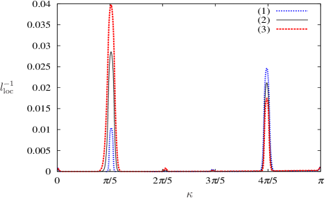
A numerical evaluation of the inverse localisation length confirms this conclusion, as can be seen from figure 1. The data represented in figure 1 were obtained for $\kappa_{1}=0.20\pi$ and $\kappa_{2}=0.21\pi$, while the mean field and the disorder strength were set equal to $U=1$ and $\sqrt{\langle u_{n}^{2}\rangle}=\sqrt{\langle\Delta_{n}^{2}\rangle}=0.05$. The long-range self-correlations (9) enhance the localisation of the electronic states in the two narrow regions $[0.20\pi,0.21\pi]$ and $[0.79\pi,0.80\pi]$ and delocalise the other states. Cross-correlations, on the other hand, modulate the localisation-delocalisation transition, making it more or less pronounced according to the sign of the $\cos\kappa\sin(2\eta)$ term in the right-hand side of (11).

Obviously, the localisation-delocalisation transition produced by long-range self-correlations has repercussions on the transmission properties of a finite aperiodic Kronig-Penney model sandwiched between two perfect leads. When the longitudinal size of the random sample is larger than the localisation length of the localised states, it is natural to expect that a continuum of delocalised states manifests itself in the form of a transparent energy window, while the regions of enhanced localisation become low-transmittivity gaps. As for cross-correlations, they can either enhance or reduce the opacity of the low-transmittivity intervals. Numerical studies confirmed this expectations [20]. They also showed that the effects of self- and cross-correlations can be detected in random samples of moderate size, as can be seen in figure 2, which represents the transmission coefficient $T$ of a random Kronig-Penney model of $N=40$ sites for a specific realisation of the disorder.

Figure 2: (Colour online) Transmission coefficient $T$ versus Bloch wavevector $\kappa$ in an aperiodic Kronig-Penney model of $N=40$ sites. The cases of total positive and negative cross-correlations are compared with the case in which cross-correlations are absent. The represented data were obtained for the same parameters of the model used in the case of figure 1, i.e., $U=1$ and $\sqrt{\langle u_{n}^{2}\rangle}=\sqrt{\langle\Delta_{n}^{2}\rangle}=0.05$.

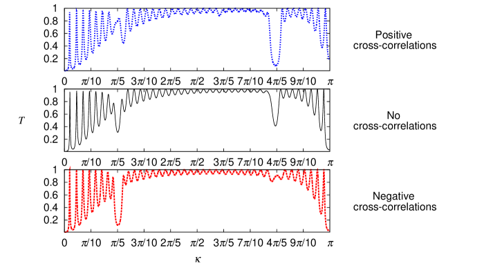
One can see that self-correlations create transmission gaps corresponding to the windows of localised states. Positive cross-correlations increase the transmittivity in the low-energy gap (almost removing the gap itself) and further reduce it in the high-energy gap, whereas for negative cross-correlations the inverse effect is observed in the two gaps. As a final comment on this issue we note that, when one considers transmission in short random samples, sample-to-sample fluctuations may prevent the transmission coefficient from following closely the behaviour of the theoretical localisation length for some disorder realisations. In the next section we will discuss how the effects of cross-correlations appear in our random waveguide.

3 Experimental setup and measurement technique

We describe the experimental setup and the measurement technique in three steps. We first present the apparatus and explain how we measured the mode-resolved microwave transport through the waveguide. Then we explain how we realised the random cross-correlated lattice inside the waveguide. Finally we discuss how the experimental band structure was related to that of the theoretical model (1) thereby establishing a functional relation between the wavevector $k_{x}$ and the Bloch vector $\kappa$.

3.1 Microwave measurement

For our experiment we used a variant of the setup employed in [23] to analyse transport in quasi-1D structures. The setup consists of a rectangular waveguide. The top plate can be lifted so that scatterers can be placed at will inside the waveguide. Figure 3 shows the waveguide with the top plate removed and four bars placed inside as an example of scattering structure.

Figure 3: (Colour online) Schematic picture of the experimental setup with top plate removed (not to scale). Brass bar inlays can be freely placed inside the waveguide. The number of bars varies according to the spacing $d_{n}$. Antennas shown here with parts of the top plate can be moved separately along the $z$-direction. The distance along the $x$-axis between the antennas is $L=1.50$ m, the total waveguide length is 2.38 m. Absorbers at the ends of the waveguide are omitted.

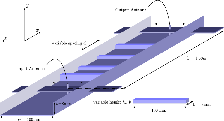
Two antennas are set at positions $x_{\mathrm{in}}=0$ and $x_{\mathrm{out}}=1.5\mbox{ m}$, with one serving as an emitter and the other as a receiver. The distance between the antennas, $L=x_{\mathrm{out}}-x_{\mathrm{in}}=1.5\mbox{ m}$ represents the effective length of the waveguide, whose width and height are $w=100\mbox{ mm}$ and $h=8\mbox{ mm}$. The antennas are plugged into the waveguide through mobile slides so that they can be moved freely from $0$ to $w$ along the transversal $z$-direction. Microwave absorbers are placed between each antenna and the corresponding end of the waveguide to avoid back-reflection from the open end. The total length of the apparatus is $2.38\mbox{ m}$.

A microwave vector network analyser allowed us to measure the transmission coefficient of the waveguide from the input antenna at $(x_{\mathrm{in}},z_{\mathrm{in}})$ to the output antenna at $(x_{\mathrm{out}},z_{\mathrm{out}})$, i.e., the scattering matrix $S(x_{\mathrm{in}},z_{\mathrm{in}};x_{\mathrm{out}},z_{\mathrm{out}})$. Because the antennas are fixed in the $x$-direction, in what follows we write $S(z_{\mathrm{in}},z_{\mathrm{out}})$ as a short-hand notation for $S(0,z_{\mathrm{in}};L,z_{\mathrm{out}})$. We measured the waveguide transmission coefficient as a function of the frequency $\nu$ for the lowest-frequency TE componentlowest-frequency transverse electric (TE) component of the electromagnetic field. In fact, for a given frequency $\nu$ there are several propagating waves with wavenumber $|k|=2\pi\nu/c$. Due to the confinement along the width of the waveguide, the $z$-component of the wavevector takes discrete values, $k_{z}^{(n)}=\pi n/w$, corresponding to propagating modes with longitudinal wavenumbers

$$k_{x}^{(n)}=\sqrt{k^{2}-(\pi n/w)^{2}}$$

with $n=1,2,\ldots,N_{w}$. The total number $N_{w}$ of propagating modes is determined by the integer part $[[\cdots]]$ of the mode parameter $kw/\pi$:

$$N_{w}=[[kw/\pi]].$$

To separate the different modes we measure $S(z_{\mathrm{in}},z_{\mathrm{out}})$ at several positions $z_{\mathrm{in}}$ and $z_{\mathrm{out}}$ distributed over the whole width $w$. The transmission between the initial point $(x=0,y_{1})$ and the final point $(x=L,y_{2})$ can be decomposed into all contributing modes

$$S(z_{\mathrm{in}},z_{\mathrm{out}})=\sum_{nm}S_{nm}\sin\left(\frac{m\pi z_{\mathrm{in}}}{w}\right)\sin\left(\frac{n\pi z_{\mathrm{out}}}{w}\right).$$ (12)

From (12) one can obtain the scattering matrix in mode representation with a twofold sine transform. The matrix element $S_{nm}$ denotes the scattering from the $m$-th to the $n$-th mode.

If all propagating modes were considered, the waveguide would correspond to a quasi-1D open strip [23], while the transmission coefficient for the first mode would be related to the scattering matrix via the identity

$$T_{1}=\sum_{n=1}^{N_{w}}|S_{1n}|^{2}.$$

However, we found that, as long as the scatterers fill homogenously the waveguide along the $z$ direction, the individual modes propagate independently of each other through the waveguide. Therefore we chose bars whose length perfectly matched the waveguide width keeping a translation invariance in the $y$ direction. In this way, as in [23], we obtained a waveguide in which the mode-mode couplings were usually negligible. This made the scattering matrix $S_{mn}$ practically diagonal (so that $T_{1}\simeq|S_{11}|^{2}$). The absence of intermodal scattering allowed us to restrict our measurements to the first propagating mode: we were thus able to put the experimental setup in correspondence with the strictly 1D theoretical model (1). Note that the equivalence of the waveguide to a 1D device did not require that the setup itself be strictly 1D.

3.2 Correlated random scattering structures

We used brass bars as scatterers in the waveguide. As explained in section 3.1, the requirement that the setup should behave as a 1D device defined the length of the scattering bars. The bar width $b=8\mbox{ mm}$ was chosen as in [23], because it is a good trade-off between small width and sufficient scattering strength. The width of the bars and the finite length of the waveguide limited the number of bars that we could insert: we formed a scattering array of 40 bars in total.

In contrast to [23], in the present case the bars were not only separated by random spacings $d_{n}$ (structural disorder), but also had random heights $h_{n}$ (compositional disorder). The bar heights spanned the range from $0.1\mbox{ mm}$ to $0.8\mbox{ mm}$ in steps of $0.1\mbox{ mm}$. We derived sequences of bar heights $h_{n}$ and spacings $d_{n}$ by scaling the corresponding variables $u_{n}$ and $\Delta_{n}$ of the Kronig-Penney model (1) which we used to obtain the transmission coefficient represented in figure 2 (see section 2). In this way we obtained two random successions $\{h_{n}\}$ and $\{d_{n}\}$ with self-correlations of the form (9) with $\kappa_{1}=0.20\pi$ and $\kappa_{2}=0.21\pi$. This choice implied a rather high value of the transmittivity for most frequencies, with a sharp drop in the two narrow gaps corresponding to the intervals $[0.20\pi,0.21\pi]$ and $[0.79\pi,0.80\pi]$ of the left half of the first Brillouin zone. As in the example discussed in section 2, in addition to long-range self-correlations, the random sequences of bar heights and spacings were cross-correlated: we considered the cases of maximally positive ($\eta=\pi/4$) and negative ($\eta=-\pi/4$) cross-correlations as well as the case in which heights and spacings of the bars were not cross-correlated ($\eta=0$).

In figure 4 we show the arrangements of the scattering bars within the waveguide for the three cases discussed. The influence of the cross-correlations is clearly visible. In fact, positive cross-correlations tend to produce large spacings between high bars, while negative cross-correlation reduce the distance separating high bars.

Figure 4: (Colour online) Profile of the scattering arrangement within the waveguide for the cases of positive (top), absent (middle), and negative (bottom) cross-correlations.

3.3 Transmission bands and Bloch vector calculation

Figure 5: (Colour online) Transmission coefficient $T_{1}$ for the first propagating mode versus wave vector $k_{x}$. The dotted line (blue) and the dashed line (red) respectively correspond to the cases of maximal positive and negative cross-correlations. The solid line (black) corresponds to the case in which no cross-correlations are present.

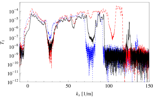
The measured transmission for the first mode versus the longitudinal wavevector is shown in figure 5. One can clearly see the first band. The band edges are the same for the cases of positive and absent cross-correlations, but in the case of negative cross-correlations the band is broader and the second gap is shifted towards higher wavenumbers $k_{x}$. Note that in all the measurements we used the same bars, which were only shuffled and put in different positions in the three cases. This means that, although the constituents of the scattering arrangements are the same, cross-correlations can broaden the transmission band. We attribute this effect to a shadowing effect. In the case of negative cross-correlations, in fact, high bars are separated by much smaller distances than in the other cases. Therefore the waves do not “feel” the same underlying lattice structure in the case of negative cross-correlations and this is probably the origin of the enlarged band.

To analyse the changes in the transmission gaps brought about by cross-correlations, we need to know the band structure of the experimental setup or, equivalently, the relation between the longitudinal wavevector $k_{x}$ and the Bloch vector $\kappa$.

We followed an empirical approach to establish a correspondence between $k_{x}$ and $\kappa$. Specifically, we associated the edges of the transmission band to the values $\kappa=0$ and $\kappa=\pi$ of the Bloch vector. We then used a linear interpolation to extend the $k_{x}-\kappa$ correspondence to the whole Brilllouin zone. This corresponds to a linear fit $\kappa=ak$, which is consistent with the fact that, as shown in [23], the finite width of the bars can be theoretically described by introducing an effective refractive index $a$ so that $k\rightarrow ak$.

4 Experimental results

The theoretical results for the Kronig-Penney model, represented by the inverse localisation length (11) and the transmission coefficient pictured in figure 2, suggest that the transmission gap in the right neighbourhood of $\kappa=\pi/5$ should be reduced or enhanced according to whether the height-position correlations are positive or negative, whereas the contrary should happen for the gap in the left neighbourhood of $\kappa=4\pi/5$. These expectations are confirmed by the experimental results, represented in figure 6, figure 7, and figure 8.

Figure 6: (Colour online) Transmission coefficient $T_{1}$ for the first propagating mode versus Bloch wavevector $\kappa$. The dotted line (blue) and the dashed line (red) respectively correspond to the cases of maximal positive and negative cross-correlations. The shaded area highlights the variation of $T_{1}$ due to cross-correlations.

Figure 7: (Colour online) Transmission coefficient $T_{1}$ for the first propagating mode versus Bloch wavevector $\kappa$. The dotted line (blue) and the solid line (black) respectively correspond to the cases of positive and absent cross-correlations. The shaded area highlights the variation of $T_{1}$ due to positive cross-correlations.

Figure 8: (Colour online) Transmission coefficient $T_{1}$ for the first propagating mode versus Bloch wavevector $\kappa$. The dashed line (red) and the solid line (black) respectively correspond to the cases of negative and absent cross-correlations. The shaded area highlights the variation of $T_{1}$ due to negative cross-correlations.

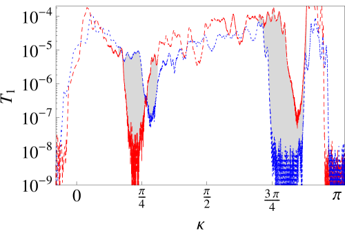
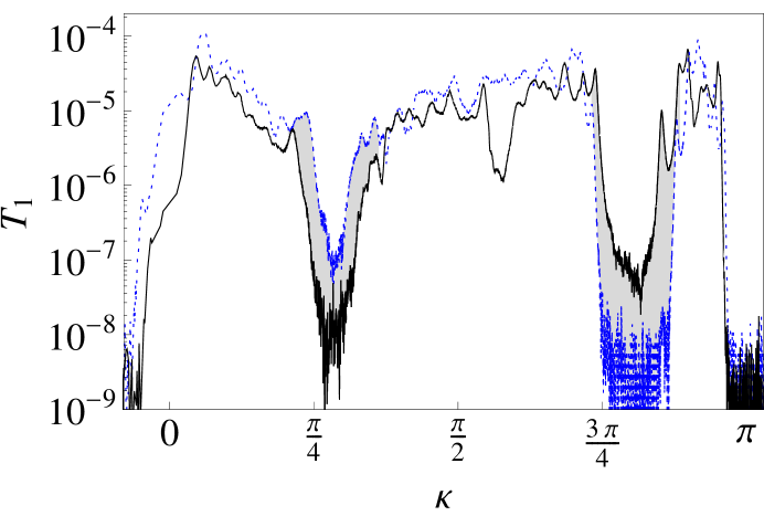
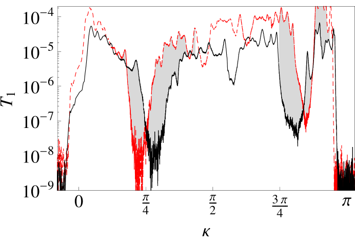
In figure 6 we show the transmission coefficient $T_{1}$ for the first propagating mode in the two extreme cases of maximum positive and negative cross-correlations between compositional and structural disorders. Figure 7 and figure 8 respectively compare the transmission coefficient $T_{1}$ in the absence of cross-correlations ($\eta=0$) with the same quantity measured when cross-correlations take the maximal positive ($\eta=\pi/4$) and negative ($\eta=-\pi/4$) values. The experimental data show that the transmission coefficient in the opaque gaps is reduced or enhanced according to the theoretical expectations. This is made particularly evident by the comparison of figure 2 and figure 6. In both cases switching from positive to negative cross-correlations decreases the transmittivity in the first opaque window and enhances it in the second gap. Figure 7 and figure 8, on the other hand, agree well with the behaviour of the inverse localisation length in the Kronig-Penney model represented in figure 1: one can easily see, for instance, that positive cross-correlations decrease localisation in the first region of localised states and enhance it in the second interval while, correspondingly, they make the first transmission gap more shallow and deepen the second one. Negative cross-correlations have the same effects, but with reversed gaps. The shift to lower (higher) frequency of the induced lower (higher) gaps in case of negative cross-correlations seen in figure 8 and in figure 6 is due to the fact that the linear rescaling using the band edge is only an approximation.

5 Conclusions

This work is the first experimental study of the effects that cross-correlations between different random potentials have on the transport properties of a 1D waveguide. We analysed the microwave transmission of the first mode in a multimode waveguide with compositional and structural disorder where no mode coupling was present. Specifically, we inserted brass bars in the waveguide which acted as scatterers and were characterised by self- and cross-correlated random heights and positions. We showed how cross-correlations between the random heights and spacings of the scatterers can modulate the transmittivity in the non-transparent frequency windows created by long-range self-correlations of the disorder. The results agree with the theoretical predictions previously obtained for an aperiodic Kronig-Penney model.

The agreement between theoretical predictions and experimental data is far from trivial, because the theoretical analysis was based on a number of simplifying assumptions, such as weak disorder and irrelevance of some experimental imperfections, e.g. absorption, which are present in any actual waveguide. Besides, the theoretical results for the transmission coefficient did not guarantee that the effect of cross-correlations would be visible also in 1D devices of reduced length. The results obtained in the present experiments, therefore, support the validity of the theoretical predictions and show that the effects of cross-correlations are not eliminated by the reduced length of the random waveguide.

References

- [1] F. A. B. F. de Moura and M. L. Lyra. Delocalization in 1D Anderson model with long-range correlated disorder. Phys. Rev. Lett., 81:3735, 1998.
- [2] F. A. B. F. de Moura and M. L. Lyra. de Moura and Lyra reply. Phys. Rev. Lett., 84:199, 2000.
- [3] F. M. Izrailev and A. A. Krokhin. Localization and the mobility edge in one-dimensional potentials with correlated disorder. Phys. Rev. Lett., 82:4062, 1999.
- [4] A. A. Krokhin and F. M. Izrailev. Anderson localization and the mobility edge in 1D random potentials with long-range correlations. Ann. Phys. (Leipzig), SI-8:153, 1999.
- [5] P. Markoš and C. M. Soukoulis. Wave Propagation: From Electrons to Photonic Crystals and Left-Handed Materials. Princeton University Press, Princeton, 2008.
- [6] D. H. Dunlap, H.-L. Wu, and P. W. Phillips. Absence of localization in a random-dimer model. Phys. Rev. Lett., 65:88, 1990.
- [7] V. Bellani, E. Diez, R. Hey, L. Toni, L. Tarricone, G. B. Parravicini, F. Domínguez-Adame, and R. Gomez-Alcala. Experimental evidence of delocalized states in random dimer superlattices. Phys. Rev. Lett., 82:2159, 1999.
- [8] U. Kuhl, F. M. Izrailev, A. A. Krokhin, and H.-J. Stöckmann. Experimental observation of the mobility edge in a waveguide with correlated disorder. Appl. Phys. Lett., 77:633, 2000.
- [9] A. Krokhin, F. Izrailev, U. Kuhl, H.-J. Stöckmann, and S. E. Ulloa. Random 1D structures as filters for electrical and optical signals. Physica E, 13:695, 2002. Conf. on Modulated Semicond. Structures (MSS 10).
- [10] J. A. Sánchez-Gil, V. Freilikher, A. A. Maradudin, and I. V. Yurkevich. Anderson localization of expanding Bose-Einstein condensates in random potentials. Phys. Rev. Lett., 98:210401, 2007.
- [11] P. Lugan, A. Aspect, L. Sanchez-Palencia, D. Delande, B. Grémaud, C. A. Müller, and C. Miniatura. One-dimensional Anderson localization in certain correlated random potentials. Phys. Rev. A, 80:023605, 2009.
- [12] P. Bouyer. Anderson localization of matter waves. Ann. Phys., 18:844, 2009.
- [13] F. M. Izrailev and N. M. Makarov. Localization in correlated bilayer structures: From photonic crystals to metamaterials and semiconductor superlattices. Phys. Rev. Lett., 102:203901, 2009.
- [14] F. M. Izrailev and N. M. Makarov. Onset of delocalization in quasi-one-dimensional waveguides with correlated surface disorder. Phys. Rev. B, 67:113402, 2003.
- [15] F. M. Izrailev, N. M. Makarov, and M. Rendón. Rough surface scattering in many-mode conducting channels: gradient versus amplitude scattering. Phys. Stat. Sol (b), 242:1224, 2005.
- [16] A. A. Krokhin, V. M. K. Bagci, F. M. Izrailev, O. V. Usatenko, and V. A. Yampol skii. Inhomogeneous DNA: Conducting exons and insulating introns. Phys. Rev. B, 80:085420, 2009.
- [17] E. L. Albuquerque, M. L. Lyra, and F. A. B. F. de Moura. Electronic transport in dna sequences: The role of correlations and inter-strand coupling. Physica A, 370:625, 2006.
- [18] J. C. Hernández Herrejón, F. M. Izrailev, and L. Tessieri. Anomalous properties of the Kronig-Penney model with compositional and structural disorder. Physica E, 40:3137, 2008.
- [19] J. C. Hernández Herrejón, F. M. Izrailev, and L. Tessieri. Anomalous localization in the aperiodic Kronig-Penney model. J. Phys. A, 43:425004, 2010.
- [20] J. C. Hernández Herrejón, F. M. Izrailev, and L. Tessieri. Electronic states and transport properties in the Kronig-Penney model with correlated compositional and structural disorder. Physica E, 42:2203, 2010.
- [21] F. M. Izrailev, A. A. Krokhin, and S. E. Ulloa. Mobility edge in aperiodic Kronig-Penney potentials with correlated disorder: Perturbative approach. Phys. Rev. B, 63:041102(R), 2001.
- [22] U. Kuhl, F. M. Izrailev, and A. A. Krokhin. Enhancement of localization in one-dimensional random potentials with long-range correlations. Phys. Rev. Lett., 100:126402, 2008.
- [23] O. Dietz, U. Kuhl, H.-J. Stöckmann, N. M. Makarov, and F. M. Izrailev. Microwave realization of quasi-one-dimensional systems with correlated disorder. Phys. Rev. B, 83:134203, 2011.