Abstract

Within the preprocessing pipeline of a Next Generation Sequencing sample, its set of Single-Base Mismatches is one of the first outcomes, together with the number of correctly aligned reads. The union of these two sets provides a $4\times 4$ matrix (called Single Base Indicator, SBI in what follows) representing a blueprint of the sample and its preprocessing ingredients such as the sequencer, the alignment software, the pipeline parameters. In this note we show that, under the same technological conditions, there is a strong relation between the SBI and the biological nature of the sample. To reach this goal we need to introduce a similarity measure between SBIs: we also show how two measures commonly used in machine learning can be of help in this context.

Introduction

A first measure of the goodness of alignment of a Next Generation Sequencing (NGS) sample is given on one side by the number of correctly aligned reads, and on the other side on the number of wrongly detected bases, collected in the single-base mismatches count. All these values are among the basic outcomes of the sample preprocessing, regardless of the ingredients of the used pipeline. These information can be grouped together in a $4\times 4$ matrix of integer values indexed by the four bases A,C,G,T, where the entry in position X,Y is the number of true bases (in the reference genome) X interpreted as Y. In what follows, we call this matrix the Single-Base Indicator, SBI for short, of the studied sample.

Obviously, the SBI is depending not only on the sample, but also on the adopted pipeline: thus, the sources of variabilities possibily affecting the final outcome are several. In fact, different alignment performance have been assessed for different software (Bowtie and BWA only to mention the two most popular ones), the preprocessing (with separated or unified lanes) and filtering procedures applied, and the sequencing platform. Thus the SBI can be seen as (a sort of) signature for the investigated sample with respect to the employed pipeline configuration, with the aim of using it to quantitatively formalize differences; for example, to be used as a baseline reference for the noise level that may be expected for a given configuration and thus, in some sense, for the stability of the configuration itself mimicking what has been carried out in [1]. To reach this goal, a similarity measure for SBI is needed: in this paper, we propose to use concepts from Statistical Machine Learning to deal with this problem, and namely the theory of classifier performance comparison.

In fact, the SBI can be seen as the confusion matrix of a classification problem on the four classes A,G,C,T, where the classifier is the alignment pipeline and the ground truth is the reference genome. Within this framework, several measures are available in literature for translating a confusion matrix into a single performance value: see for instance [2, 3, 4] for a review of the more classical methods, or [5] for novel measures or [6, 7, 8] for totally different approaches. Among others, the Matthews Correlation Coefficient (MCC, for short) has recently attracted the attention of many researchers in the field: in particular, it has been designed as the elective measure in initiatives defining methodologic guidelines such as MAQC-II [9] led by the U.S. Food and Drug Administration (FDA). Originally introduced for binary problems [10], its generalization to the multiclass case was defined in [11] and since then used in a wide range of tasks. Here the (generalized) MCC is used to summarize in a unique real value the quality of the alignment of a sample: the range of the values is $[-1,1]$ and the higher the value the better the alignment, with 1 representing the ideal situation of no mismatch occurring.

In addition to the comparison with a common ideal situation, it is worthwhile to consider the mutual similarities and differences between SBIs: we perform this by looking at each SBI as a (nominal) histogram, and use a suitable distance. Among the many available distances [12, 13], we chose to use the Canberra distance [14]. This is motivated by the fact that, being defined as the ratio between the (absolute value) of the difference and the sum of two quantities, the Canberra distance is intrinsically more susceptible to even slight changes around zero. This case is indeed the one we are interested in, since when considering the (frequency) histogram corresponding to a SBI, the values inherited by the single-base mismatches are very close to zero because of the preponderance of the occurrences of the exact matches.

As an application of these two similarity measures, we show the evaluation of the alignment of a NGS dataset where all the components of the pipeline are fixed, yielding the tissue type as the sole controlled source of variability. The analysis with both MCC and Canberra distance leads to the hypothesis that there is a strong relation between the tissue type and the corresponding SBI structures, thus representing a first promising step towards the development of a stability theory for NGS data through the SBI.

Materials and Methods

Deep sequencing data

A NGS data set, denoted here as “BM1”, was used as testbed for evaluating the proposed method. The data set, previously described in [15] and available on EMBL-EBI European Nucleotide Archive (ENA) with accession number SRP000727, consists of deep transcriptome sequencing (RNA-seq) of 11 human tissues and 6 cell lines. The biological samples were sequenced on the Illumina Genome Analyzer (Illumina, Inc., San Diego, CA, USA), obtaining over 400 million short (32 bp) reads. In case a biological sample was sequenced over multiple lanes, in the following we refer to each single lane as a sample. The data considered here include a total of 103 samples (lanes) distributed as in Table 1.

Alignment and postprocessing

The short reads were mapped to the reference human genome (UCSC assembly hg18, NCBI Build GRCh36.1), including unordered sequences and alternate haplotypes, with either BWA 0.5.7 [16] (alignment A1), bowtie 0.12.5 [17] (alignment A2), and TopHat 1.1.4 [18] (alignment A3). The mapping was performed allowing at most two nucleotide differences (i.e., mismatches or gaps) over the read length.

For each tissue or cell line and for each alignment method, a consensus sequence of the whole genome (i.e., a genetic sequence of mapped regions, including variants) was called from read mappings using SAMtools 0.1.7a [19] with the model implemented in MAQ [20]. Small variants (i.e., single-base mismatches) were subsequently called from the consensus sequences and filtered according to read coverage and mapping quality constraints. In detail, only variants with a mapping Phred quality score larger than 30 and covered by at least 3 (to prevent spurious calls) and at most 100 reads (to avoid calls in regions with very high depth) were kept, following guidelines commonly adopted in the literature [21, 22] and suggested by Illumina, Inc. for small variant discovery [23]. Finally, we computed an additional “virtual sample” by merging the alignments of different lanes, when present.

Single Base Indicator

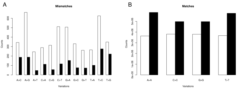
A typical outcome of any alignment software is a summary of the exact matches and the occurring single-base mismatches, and these information may appear under very different shapes. For our purposes, we are interested in collecting (for each sample, or lane $s$) the 16 integer values $X>Y$ counting the number of times the base $X$ in the reference genome has been read as $Y$ by the alignemnt pipeline, where $X,Y\in\mathcal{B}=\{A,C,G,T\}$. The 16 values are then organized in a square matrix $\textrm{SBI}(s)\in\mathcal{M}(|\mathcal{B}^{2}|,\mathbb{N})$, called Single Base Indicator (SBI), or as a nominal (i.e., with no ordering among the 16 categories $X>Y$) histogram, possibily normalized over the total number of counts $\displaystyle{\textrm{TC}=\sum_{i,j\in\mathcal{B}}\textrm{SBI}(s)_{ij}}$. An example of two SBI histograms is shown in Figure 1, respectively for the two samples SRR015311 (skeletal muscle tissue) and SRR015286 (mixed brain tissue) in BM1.

Distance from perfect alignment

Starting from the SBI matrix, define two matrices $X,Y\in\mathcal{M}(\textrm{TC}\times|\mathcal{B}|,\mathbb{F}_{2})$ where $X_{sn}=1$ if the base $s$ is predicted to be of class $n$ ($\textrm{pc}(s)=n$) and $X_{sn}=0$ otherwise, and $Y_{sn}=1$ if base $s$ belongs to class $n$ ($\textrm{tc}(s)=n$) and $0$ otherwise. Using Kronecker’s delta function, the definition becomes:

$$X=\left(\delta_{\textrm{pc}(s),n}\right)_{sn}\quad Y=\left(\delta_{\textrm{tc}(s),n}\right)_{sn}\ .$$

Then the Matthews Correlation Coefficient MCC can be defined as the ratio:

$$\textrm{MCC}=\frac{\textrm{cov}(X,Y)}{\sqrt{{\textrm{cov}(X,X)}\cdot{\textrm{cov}(Y,Y)}}}\ ,$$

where $\textrm{cov}(\cdot,\cdot)$ is the covariance function. In terms of the matrix SBI, the above equation can be written as:

$$\frac{\displaystyle{\sum_{k,l,m=1}^{N}\textrm{SBI}_{kk}\textrm{SBI}_{ml}-\textrm{SBI}_{lk}\textrm{SBI}_{km}}}{\sqrt{\displaystyle{\sum_{k=1}^{N}}\left(\displaystyle{\sum_{l=1}^{N}}\textrm{SBI}_{lk}\right)\left(\displaystyle{\sum_{\begin{subarray}{c}f,g=1\\ f\not=k\end{subarray}}^{N}}\textrm{SBI}_{gf}\right)}\sqrt{\displaystyle{\sum_{k=1}^{N}}\left(\displaystyle{\sum_{l=1}^{N}}\textrm{SBI}_{kl}\right)\left(\displaystyle{\sum_{\begin{subarray}{c}f,g=1\\ f\not=k\end{subarray}}^{N}}\textrm{SBI}_{fg}\right)}}$$

MCC lives in the range $[-1,1]$, where $1$ is perfect classification, $-1$ is reached in the alternative extreme misclassification case of a confusion matrix with all zeros but in two symmetric entries $\textrm{SBI}_{\bar{i},\bar{j}}$, $\textrm{SBI}_{\bar{j},\bar{i}}$, and $0$ when the confusion matrix is all zeros but for one single column (all samples have been classified to be of a class $k$), or when all entries are equal $\textrm{SBI}_{ij}=K\in\mathbb{N}$. Note that MCC is invariant with respect to multiplication of all SBI’s entries by a constant.

Canberra distance between SBIs

Given the histogram (normalized over the respective TC) of the SBI for two samples $s,t$ it is possible to define their Canberra distance as follows:

$$\textrm{Ca}(s,t)=\sum_{i,j\in\mathcal{B}}\frac{|\textrm{SBI}(s)_{ij}-\textrm{SBI}(t)_{ij}|}{\textrm{SBI}(s)_{ij}+\textrm{SBI}(t)_{ij}}\ .$$

Because of the shape of the denominator, variations on the mismatch categories tend to get higher weight in the sum than the exact matches, thus highlighting the differences on the wrongly assigned bases of the two compared samples.

Sammon’s mapping

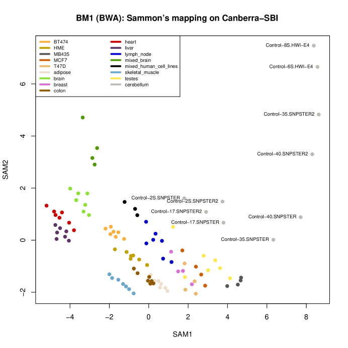
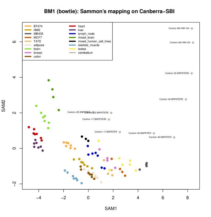
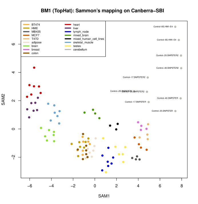
The projection of SBIs into a two-dimensional space was carried out by the nonlinear scaling algorithm proposed by Sammon[24], using $\textrm{Ca}(s,t)$ as the distance function. The mapping is achieved by minimizing the Sammon stress function, which in our terms is defined as

$$\textrm{E}=\frac{1}{\sum_{s\not=t}\textrm{Ca}^{*}(s,t)}\sum_{s\not=t}\frac{\left(\textrm{Ca}^{*}(s,t)-\textrm{Ca}(s,t)\right)^{2}}{\textrm{Ca}^{*}(s,t)}$$

where $\textrm{Ca}^{*}(s,t)$ is the Canberra distance of samples $s,t$ in the original space and $\textrm{Ca}(s,t)$ is the Canberra distance in the projected space.

Results

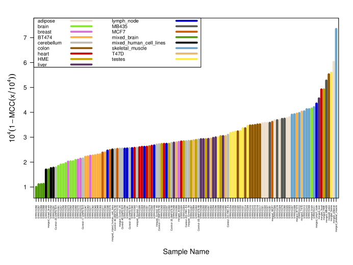
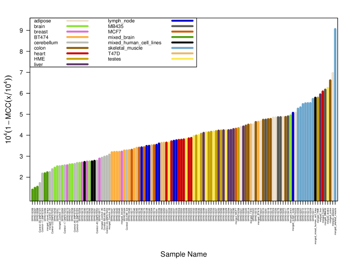
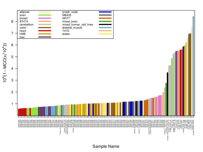
The first part of the analysis consists in computing the MCC values for all the elements of the data set. In order to speed up computations and to ease data handling, the SBI matrices are loaded in a portable SQLite database. To better highlight differences, in Figures 2 (alignment A1), 4 (alignment A2) and 6 (alignment A3) we ordered the 123 samples (including 24 virtual samples) of data set BM1 for decreasing MCC and displayed on the $y$ axes the quantity $10^{4}(1-\textrm{MCC})$; thus, the smaller the numbers (leftmost samples), the closer the SBI to the perfect alignment case. The main observation here is that samples belonging to the same class tend to have very similar MCC values, and thus to group together in the plot: in Tables 2, 3 and 4 we list the rank of all BM1 samples grouped by class and sorted in decreasing MCC order, for alignments A1, A2 and A3. The samples of the brain class are the best aligned in average, with mixed brain (whose tissue is biogically close to brain tissue) ranking first for A1 and A2. On the other hand, almost all the merged virtual samples have the worst alignment quality in terms of number of single-base mismatches.

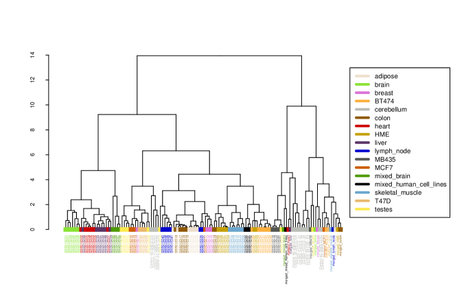
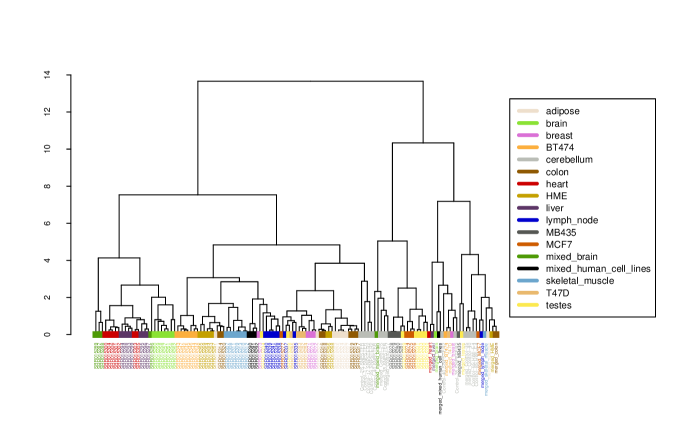
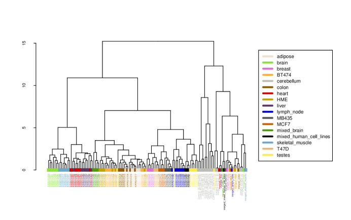
These claims are furthermore supported by the dendrogram in Figure 3, where the mutual 123 Canberra distances among SBI histograms from alignment A1 are hierarchically clustered together with complete linkage: Table 5 summarizes the structure of the clusters resulting by cutting the dendrogram at height 2. Similar results are reported for alignments A2 (Fig. 5, Tab. 6) and A3 (Fig. 7, Tab. 7). Again, for many classes, samples in the same class are consistently grouped together, with the merged lanes virtual samples forming a separate entity.

In both analyses, samples of the same class tend to quantitatively show an intrinsinc similarity. This result seems to support our claim that the SBI mismatch profile associated to a sample is strongly dependent on its tissue type, when all other sources of variability within the preprocessing pipeline are kept stable.

Sammon’s mapping of all BM1 samples using Canberra distance between SBIs (Figures 8, 9, 10) shows how technical replicates form well-defined clusters stratified by tissue types, while a separate trend exists for the biological replicates (cerebellum samples), as expected.

Conclusions

We propose candidate indicators for profiling RNA-seq experiments based on generalized MCC and Canberra distance. The goal is to assess whether variability in RNA-Seq experiments depends on factors that resemble the analogous of “batch effects” for microarrays.

Indicators are built on top of single-base mismatches, which are a first direct measurement of the goodness of alignment. Results show that the proposed indicators make it possible to identify (sub)structures of data determined by underlying experimental characteristics such as tissue types, paving the way for a normalization method for NGS that could guarantee the reproducibility of results, as being nowadays explored by initiatives such as the Sequencing Quality Control (SEQC) led by U.S. FDA.

The study is currently being extended to consider multiple NGS platforms, such as Illumina, Helicos, and SOLiD.

Figure Legends

Figure 1: Alignment A1: histogram of the SBI for the two BM1 samples SRR015311 (skeletal muscle tissue, in white) and SRR015286 (mixed brain tissue, in black) with different scales for the 12 single-base mismatches categories (A) and the 4 exact matches categories (B).

Figure 2: NGS samples of data set BM1 (alignment A1) ranked according to increasing value of zoomed generalized MCC and colored according to their class: leftmost samples are closer to the ideal situation of zero mismatches.

Figure 3: Data set BM1, alignment A1: dendrogram of 123 NGS samples (colored according to their class) hierarchically clustered (complete linkage) by Canberra distance.

Figure 4: NGS samples of data set BM1 (alignment A2) ranked according to increasing value of zoomed generalized MCC and colored according to their class: leftmost samples are closer to the ideal situation of zero mismatches.

Figure 5: Data set BM1, alignment A2: dendrogram of 123 NGS samples (colored according to their class) hierarchically clustered (complete linkage) by Canberra distance.

Figure 6: NGS samples of data set BM1 (alignment A3) ranked according to increasing value of zoomed generalized MCC and colored according to their class: leftmost samples are closer to the ideal situation of zero mismatches.

Figure 7: Data set BM1, alignment A3: dendrogram of 123 NGS samples (colored according to their class) hierarchically clustered (complete linkage) by Canberra distance.

Figure 8: Sammon map of BM1 samples (alignment A1) using Canberra distance between SBIs: cerebellum samples are highlighted.

Figure 9: Sammon map of BM1 samples (alignment A2) using Canberra distance between SBIs: cerebellum samples are highlighted.

Figure 10: Sammon map of BM1 samples (alignment A3) using Canberra distance between SBIs: cerebellum samples are highlighted.

Tables

Table 1: Samples and classes (T: tissues, CL: cell lines) for BM1 data set

Type	Class	Samples	Notes
T	adipose	7
T	brain	7
T	breast	4
T	colon	7
T	heart	7
T	liver	7
T	lymph node	7
T	mixed brain	4
T	skeletal muscle	7
T	testes	7
T	cerebellum	10	6 biological samples: 2 x 1 lane, 4 x 2 lanes
CL	BT474	7	Breast tumor
CL	HME	7	Mammary epithelial
CL	MB435	4	Estrogen-ind. breast carcinoma
CL	MCF7	4	Breast adenocarcinoma
CL	T47D	4	Ductal breast epithelial tumor
CL	mixed human cell lines	3	Breast tumor

For each class, a virtual sample is added, consisting of the merged lanes.

Table 2: Alignment A1: ranking of the samples of each class in decreasing MCC order

Class	Rank
mixed brain	1,2,3,4,6
mixed human cell lines	5,7,8,32
cerebellum	9,20,33,35,36,39,42,50,51,56,62,63,67,79
brain	10,11,12,13,15,16,17,113
breast	14,18,19,23,59
BT474	21,22,24,25,26,27,29,107
MCF7	28,31,34,47,97
lymph node	30,37,38,40,45,49,54,115
heart	41,43,44,46,48,53,60,117
HME	52,55,61,64,66,70,76,118
liver	57,68,69,71,73,74,77,116
T47D	58,65,72,78,109
testes	75,80,81,82,84,85,87,121
colon	83,86,88,89,90,91,92,120
adipose	93,94,95,98,100,103,104,122
MB435	96,99,101,102,119
skeletal muscle	105,106,108,110,111,112,114,123

Italic: merged lanes virtual sample.

Table 3: Alignment A2: ranking of the samples of each class in decreasing MCC order

Class	Rank
mixed brain	1,2,3,6,7
cerebellum	4,5,8,9,12,14,18,19,27,29,30,31,32,39
brain	10,11,13,16,17,20,24,105
breast	15,21,23,28,37
mixed human cell lines	22,25,26,115
BT474	33,34,35,36,38,40,42,92
MCF7	41,44,46,50,83
T47D	43,49,53,54,89
lymph node	45,47,48,51,52,58,59,106
heart	55,57,60,61,62,64,65,118
testes	56,63,66,68,71,74,79,120
HME	67,69,72,73,75,77,84,116
liver	70,76,78,80,81,82,86,117
adipose	85,90,93,98,99,102,107,122
colon	87,88,91,94,96,97,103,121
MB435	95,100,101,104,119
skeletal muscle	108,109,110,111,112,113,114,123

Italic: merged lanes virtual sample.

Table 4: Alignment A3: ranking of the samples of each class in decreasing MCC order

Class	Rank
heart	1,2,3,4,5,6,9,114
brain	7,8,10,11,12,13,14,108
liver	15,16,17,18,19,22,23,111
skeletal muscle	20,21,24,25,26,28,32,123
mixed brain	27,31,38,40,104
testes	29,37,45,49,60,61,69,119
cerebellum	30,33,34,35,39,82,85,92,93,103,106,107,109,110
BT474	36,41,43,48,52,56,59,113
HME	42,44,46,47,51,54,70,117
lymph node	50,53,63,75,79,80,86,116
colon	55,57,64,66,67,68,72,121
adipose	58,62,65,71,73,77,88,122
mixed human cell lines	74,83,87,105
MB435	76,78,81,84,120
MCF7	89,90,91,95,115
breast	94,97,99,100,112
T47D	96,98,101,102,118

Italic: merged lanes virtual sample.

Table 5: Alignment A1: elements (classwise) of the 24 clusters emerging by cutting the whole dendrogram at height 2.

Cluster	Elements
1	Brain
2	Heart, Liver
3	1 Mixed brain
4	3 Mixed brain
5	1 Breast, 3 MCF7, T47D, 5 Testes
6	1 Cerebellum
7	3 Cerebellum
8	5 Lymph node, 1 Testes
9	5 Colon, Adipose
10	3 Breast, 1 MCF7, 2 Lymph Node
11	5 HME, 2 Colon, Skeletal muscle
12	Mixed human cell lines
13	BT474, 2 HME
14	1 Testes, MB435
15	Mixed brain, Mixed human cell lines
16	Liver, Heart
17	1 Cerebellum
18	2 Cerebellum, 1 Cerebellum
19	2 Cerebellum, 1 Cerebellum
20	MB435, Testes
21	1 Cerebellum, Breast, Brain
22	1 Cerebellum, MCF7, BT474, T47D
23	Skeletal muscle
24	Lymph node, HME, Colon, Adipose

Bold: all elements of the class are included in the cluster; Italic: cluster includes the merged lanes virtual sample.

Table 6: Alignment A2: elements (classwise) of the 23 clusters emerging by cutting the whole dendrogram at height 2.

Cluster	Elements
1	3 Mixed brain
2	Heart, Liver
3	1 Mixed brain
4	Brain
5	BT474
6	5 HME, 1 Adipose, 2 Colon, Skeletal muscle
7	1 Breast, Mixed human cell lines, 5 Lymph node, 1 Testes
8	3 Breast, 1 MCF7, T47D, 2 Lymph node, 1 Testes
9	2 HME, 6 Adipose, 5 Colon
10	1 Cerebellum
11	3 Cerebellum
12	1 Cerebellum
13	Mixed brain, 2 Cerebellum, 1 Cerebellum
14	1 Testes, MB435
15	3 MCF7, 4 Testes
16	Liver, Heart
17	Brain, Mixed human cell lines
18	1 Cerebellum
19	1 Cerebellum, Breast, T47D, BT474
20	MB435, Testes
21	2 Cerebellum, 2 Cerebellum
22	MCF7, Lymph node
23	1 HME, 1 Colon, 1 Adipose, 1 Skeletal muscle

Bold: all elements of the class are included in the cluster; Italic: cluster includes the merged lanes virtual sample.

Table 7: Alignment A3: elements (classwise) of the 32 clusters emerging by cutting the whole dendrogram at height 2.

Cluster	Elements
1	Brain
2	Skeletal muscle
3	1 Heart
4	5 Heart, 1 Liver
5	1 Heart, 6 Liver
6	1 Mixed brain
7	3 Mixed brain
8	5 BT474, 6 HME
9	1 Testes
10	Colon, 2 BT474, Adipose, 1 HME
11	4 Breast, T47D
12	3 MCF7
13	MB435, 1 MCF7
14	1 Testes, 1 Lymph node
15	6 Lymph node
16	Mixed human cell lines
17	5 Testes
18	2 Cerebellum
19	2 Cerebellum
20	2 Cerebellum
21	1 Cerebellum
22	1 Cerebellum
23	2 Cerebellum
24	Testes
25	2 Cerebellum
26	Liver, Heart
27	Mixed human cell lines
28	Breast, MCF7, Lymph node, T47D, MB435
29	BT474, HME, Colon, Adipose
30	2 Cerebellum
31	Brain
32	Skeletal muscle

Bold: all elements of the class are included in the cluster; Italic: cluster includes the merged lanes virtual sample.

References

- 1. Jurman G, Merler S, Barla A, Paoli S, Galea A, et al. (2008) Algebraic stability indicators for ranked lists in molecular profiling. Bioinformatics 24: 258–264.
- 2. Felkin M (2007) Comparing Classification Results between N-ary and Binary Problems, Springer-Verlag, volume 43. pp. 277–301.
- 3. Sokolova M, Lapalme G (2009) A systematic analysis of performance measures for classification tasks. Information Processing and Management 45: 427–437.
- 4. Ferri C, Hernández-Orallo J, Modroiu R (2009) An experimental comparison of performance measures for classification. Pattern Recognition Letters 30: 27–38.
- 5. Wei JM, Yuan XJ, Hu QH, Wang SQ (2010) A novel measure for evaluating classifiers. Expert Systems with Applications 37: 3799–3809.
- 6. Landgrebe TC, Duin RP (2008) Efficient multiclass ROC approximation by decomposition via confusion matrix perturbation analysis. IEEE Transactions Pattern Analysis Machine Intelligence 30: 810–822.
- 7. Freitas COA, De Carvalho JM, Oliveira JJ Jr, Aires SBK, Sabourin R (2007) Confusion matrix disagreement for multiple classifiers. In: Rueda L, Mery D, Kittler J, editors, Proceedings of 12th Iberoamerican Congress on Pattern Recognition, CIARP 2007, LNCS 4756. Springer-Verlag, pp. 387–396.
- 8. Freitas COA, De Carvalho JM, Oliveira JJ Jr, Aires SBK, Sabourin R (2007) Distance-based Disagreement Classifiers Combination. In: Proceedings of the International Joint Conference on Neural Networks, IJCNN 2007. IEEE, pp. 2729–2733.
- 9. The MicroArray Quality Control (MAQC) Consortium (2010) The MAQC-II Project: A comprehensive study of common practices for the development and validation of microarray-based predictive models. Nature Biotechnology 28: 827–838.
- 10. Matthews BW (1975) Comparison of the predicted and observed secondary structure of T4 phage lysozyme. Biochimica et Biophysica Acta - Protein Structure 405: 442–451.
- 11. Gorodkin J (2004) Comparing two k-category assignments by a k-category correlation coefficient. Computational Biology and Chemistry 28: 367–374.
- 12. Cha SH, Srihari S (2002) On Measuring the Distance between Histograms. Pattern Recognition 35: 1355–1370.
- 13. Cha SH (2008) Taxonomy of Nominal Type Histogram Distance Measures. In: Proc. American Conference on Applied Mathemathics, MATH08. WSEAS, pp. 325–330.
- 14. Lance G, Williams W (1967) Mixed-Data Classificatory Programs I - Agglomerative Systems. Aust Comput J 1: 15–20.
- 15. Wang ET, Sandberg R, Luo S, Khrebtukova I, Zhang L, et al. (2008) Alternative isoform regulation in human tissue transcriptomes. Nature 456: 470–476.
- 16. Li H, Durbin R (2009) Fast and accurate short read alignment with Burrows-Wheeler transform. Bioinformatics 25: 1754–1760.
- 17. Langmead B, Trapnell C, Pop M, Salzberg SL (2009) Ultrafast and memory-efficient alignment of short DNA sequences to the human genome. Genome Biology 10: R25.
- 18. Trapnell C, Pachter L, Salzberg SL (2009) TopHat: discovering splice junctions with RNA-Seq. Bioinformatics 25: 1105.
- 19. Li H, Handsaker B, Wysoker A, Fennell T, Ruan J, et al. (2009) The sequence alignment/Map format and SAMtools. Bioinformatics 25: 2078–2079.
- 20. Li H, Ruan J, Durbin R (2008) Mapping short DNA sequencing reads and calling variants using mapping quality scores. Genome research 18: 1851–1858.
- 21. Wendl MC, Wilson RK (2008) Aspects of coverage in medical DNA sequencing. BMC bioinformatics 9: 239.
- 22. Ng SB, Turner EH, Robertson PD, Flygare SD, Bigham AW, et al. (2009) Targeted capture and massively parallel sequencing of 12 human exomes. Nature 461: 272–276.
- 23. Winn-Deen E (2010). A platform approach to translational cancer discovery and diagnostic development. Oral presentation at IlluminaDx Seminar Series.
- 24. Sammon JW Jr (1969) A nonlinear mapping for data structure analysis. Computers, IEEE Transactions on 100: 401–409.
- 25. R Development Core Team (2010) R: A Language and Environment for Statistical Computing. R Foundation for Statistical Computing, Vienna, Austria. URL http://www.R-project.org. ISBN 3-900051-07-0.