Thermalization in a one-dimensional integrable system

Abstract

We present numerical results demonstrating the possibility of thermalization of single-particle observables in a one-dimensional system, which is integrable in both the quantum and classical (mean-field) descriptions (a quasicondensate of ultracold, weakly interacting bosonic atoms are studied as a definite example). We find that certain initial conditions admit the relaxation of single-particle observables to the equilibrium state reasonably close to that corresponding to the Bose-Einstein thermal distribution of Bogoliubov quasiparticles.

I Introduction

A one-dimensional (1D) system of identical bosons with contact interactions is known to be integrable since Lieb and Liniger have solved analytically the corresponding quantum problem by means of Bethe ansatz LL . In the weakly interacting limit, this system can be described in the mean-field approximation by the Gross-Pitaevskii equation (GPE), also known as the nonlinear Schrödinger equation (NLSE). Zakharov and Shabat ZS73 have demonstrated that the NLSE with defocusing nonlinearity (which corresponds to the repulsive interactions between particles) is integrable by the inverse scattering transform (see ISTM for a general review of the inverse scattering transform method). Since the number of integrals of motion in an integrable system equals to the number of degrees of freedom (infinite in the continuous mean-field description ZS73 or equal to the number of particles in the quantum Lieb-Liniger model LL ), one might expect that the finally attained equilibrium state must still bear signatures of the initial conditions.

One-dimensional bosonic systems have been experimentally implemented with ultra-cold atoms on atom chips H1 ; H2 , with the radial trapping frequency being $\sim 10^{3}$ times higher than the longitudinal one. The ultracold degenerate atomic system (quasicondensate, i.e. a system describable by a macroscopic wave function with a fluctuating local phase) was in the 1D regime since both the temperature and the mean interaction energy per atom were well below the energy interval between the ground and the first excited states of the radial motion. The fact that the static and dynamic correlation properties of these systems were in a very good agreement with the Bose-Einstein equilibrium distribution of quasiparticles seemed to be in contradiction with the system integrability and called for explanation. To explain the observed relaxation of single- and two-particle distribution functions for the elementary excitations (Bogoliubov quasiparticles) to the Bose-Einstein equilibrium, a mechanism of integrability breakdown via three-body effective collisions involving virtual excitations of the radial degrees of freedom has been proposed M089 .

In the present paper we numerically show the existence of a certain case of nonequilibrium initial conditions of the GPE, which provide a very fast relaxation of the simplest (single-particle) observables to an equilibrium state very close to thermal equilibrium, despite the integrability of the problem.

Some indications of thermalization in 1D bosonic systems have been obtained in numerical simulations of various physical processes in quasicondensates, such as the subexponential decay of coherence between coherently split quasicondensates Stim1 , soliton formation in a 1D bosonic system in the course of (quasi)condensation DZW , in-trap density fluctuations Proukakis1 , wave chaos wchaos , and condensate formation after the addition of a dimple to a weak harmonic longitudinal confinement of a 1D ultracold atomic gas Proukakis2 . However, a systematic study of thermalization of the GPE solution in the course of time evolution was lacking up to now. Even Burnett1 , where thermalization of the GPE solution with the initial conditions corresponding to the high-temperature limit has been numerically obtained, states that formal and systematic understanding of the problem is still incomplete. We fill this gap, at least to a certain extent, with our present study.

We also have to draw a clear distinction between our approach and that of Rigol et al. Rigol1 , who theoretically studied dephasing in a quantum system of hard-core bosons on a lattice, prepared initially in a coherent superposition of eigenstates, and its relaxation to a generalized Gibbs (fully constrained) equilibrium. Our aim is to demonstrate that a weakly interacting 1D degenerate bosonic gas can approach, in the course of its evolution, a state that is reasonably close to the conventional thermal Bose-Einstein equilibrium.

II Numerical approach

We solve the GPE

$$i\hbar\frac{\partial}{\partial t}\Psi(x,t)=-\frac{\hbar^{2}}{2m}\frac{\partial^{2}}{\partial x^{2}}\Psi(x,t)+g|\Psi(x,t)|^{2}\Psi(x,t),$$ (1)

where $\Psi(x,t)$ is a classical complex field representing a quasicondensate of atoms with mass $m$ and $g$ is the effective coupling constant in one dimension (we assume $g>0$). The interaction strength is characterized by the Lieb-Liniger parameter LL $\gamma=mg/(\hbar^{2}\bar{n})\equiv(\bar{n}\xi)^{-2}$, where $\xi$ is the quasicondensate healing length and $\bar{n}\equiv\langle|\Psi(x,t)|^{2}\rangle$ is the mean 1D number density. We consider the weak interaction limit $\gamma\ll 1$. We assume periodic boundary conditions for $\Psi(x,t)$, with the period $L$ being long enough to ensure the loss of correlations over the half period: $\langle\Psi^{*}(x,t)\Psi(x+L/2,t)\rangle\ll\bar{n}$. The angle brackets denote here averaging over the ensemble of realizations. For each realization the initial conditions are prepared in a manner similar to the truncated Wigner approach TW but taking into account thermal fluctuations only (cf. Ref. Stim1 ). We express the macroscopic order parameters in terms of the phase $\phi$ and density $\delta n$ fluctuations: $\Psi=(\bar{n}+\delta n)^{1/2}e^{i\phi}$. The initial (at $t=0$) fluctuations are expanded into plane waves as

$$\delta n(x,0) = 2\sqrt{\bar{n}/L}\sum_{k\neq 0}\beta_{k}\sqrt{\eta_{k}/\epsilon_{k}}\cos(kx+\varpi_{k}),$$

$$\phi(x,0) = (1/\sqrt{\bar{n}L})\sum_{k\neq 0}\beta_{k}\sqrt{\epsilon_{k}/\eta_{k}}\sin(kx+\varpi_{k}),$$ (2)

where $\epsilon_{k}=\sqrt{\eta_{k}(\eta_{k}+2g\bar{n})}$ is the energy of the elementary (Bogoliubov) excitation with the momentum $\hbar k$ and $\eta_{k}=(\hbar k)^{2}/(2m)$. The real numbers $\beta_{k}$ and $\varpi_{k}$ have the meaning of the scaled amplitude and the offset of the thermally excited elementary wave with the momentum $\hbar k$ at $t=0$. The values of $\varpi_{k}$ are taken as (pseudo)random numbers uniformly distributed between 0 and $2\pi$. Each ensemble of realizations is also characterized by a distribution of the $\beta_{k}$ values with $\langle\beta_{k}^{2}\rangle$ being equal to the main number ${\cal N}_{0}(k)$ of elementary excitation quanta (quasiparticles) in the given mode prim1 . In equilibrium at the temperature $T$ the populations of the bosonic quasiparticle modes are given by ${\cal N}_{\mathrm{BE}}(k,T)=\{\exp[\epsilon_{k}/(k_{\mathrm{B}}T)]-1\}^{-1}$.

The use of the classical field (GPE) approach is justified, as it has been shown SMSM that the noise and correlations in an atomic quasicondensate are dominated by thermal (classical) fluctuations under experimentally feasible conditions, and the observation of quantum noise is a challenging task that can be solved in particular regimes by means of involved experimental tools Armijo .

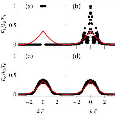
Figure 1: (Color online) Dots: mean energy per mode (scaled to $k_{\mathrm{B}}T_{0}$ with $k_{\mathrm{B}}T_{0}=2\,g\bar{n}$) as the function of wavenumber $k$ (scaled to $\xi$) for the dimensionless time $g\bar{n}t/\hbar=$ (a) 0, (b) 50, (c) 2850, and (d) 5750. The Lieb-Liniger parameter $\gamma=5\times 10^{-3}$, $k_{0}\xi=0.33$. Solid line: mean energy per mode $\epsilon_{k}{\cal N}(k,T_{\mathrm{eq}})$ for the equilibrium state, $T_{\mathrm{eq}}=0.35\,T_{0}$; see Eq. (4). The data are averaged over 200 realizations. Units on the axes in this figure and the subsequent figures are dimensionless.

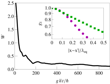
Figure 2: (Color online) Numerically obtained energy-weighted squared deviation of the quasiparticle distribution from the Bose-Einstein thermal equilibrium as a function of time. The initial energy distribution and other parameters are the same as in Fig. 1(a). The inset shows the numerically calculated first-order correlation function $g_{1}(x-x^{\prime})$ (shown on the logarithmic scale) for the dimensionless time $g\bar{n}t/\hbar=$ 0 (circles) and 6000 (squares). The distance is scaled to $\lambda_{\mathrm{eq}}$.

To integrate Eq. (1), we used the fourth-order time-splitting Fourier spectral method Thalhammer , which is rather similar to that used in Ref. Stim1 .

We have found a set of examples of solutions of Eq. (1) that demonstrate quite a good degree of thermalization. Efficient thermalization has been observed in the cases of initial population of Bogoliubov modes within a certain momentum band around $k=0$ [for simplicity, we assume ${\cal N}_{0}(k)={\cal N}_{0}(-k)$], with the bandwidth being narrow enough to ensure the phononic nature of these excitations, $|k|\xi\lesssim 1$. In Fig. 1, we present our results of numerical integration of Eq.  (1) for the initial conditions corresponding to the truncated classical distribution, parametrized by the effective temperature $T_{0}$ and the cutoff momentum $\hbar k_{0}$, i.e., for ${\cal N}_{0}(k)$ being equal to $k_{\mathrm{B}}T_{0}/\epsilon_{k}$ for $|k|<k_{0}$ and zero otherwise. For the sake of convenience, in Fig. 1 we plot the mean energy per mode $E_{k}=\epsilon_{k}{\cal N}(k)$, which does not diverge at $k\rightarrow 0$, in contrast to the time-dependent population distribution ${\cal N}(k)$. Practically, $E_{k}$ can be calculated by averaging over the ensemble of realizations the energy stored in the given mode:

$$E_{k}=\left\langle\frac{m}{2}\bar{n}|v_{k}|^{2}+\left(\frac{\hbar^{2}k^{2}}{8m\bar{n}}+\frac{g}{2}\right)|\delta n_{k}|^{2}\right\rangle,$$ (3)

where $\delta n_{k}$ and $v_{k}$ are the Fourier transforms of the density $\delta n(x,t)$ and velocity $v(x,t)=(\hbar/m)\partial\phi/\partial x$ fluctuations.

Elementary excitations at different momenta are found to be uncorrelated for all propagation times, i.e., $\langle\delta n_{k^{\prime}}\delta n_{k}^{*}\rangle=\langle|\delta n_{k}|^{2}\rangle\delta_{k\,k^{\prime}}$ and $\langle v_{k^{\prime}}v_{k}^{*}\rangle=\langle|v_{k}|^{2}\rangle\delta_{k\,k^{\prime}}$, as expected for a thermal equilibrium state.

The energy distribution approaches its equilibrium, which is quite close to the thermal Bose-Einstein distribution. The main difference is that the former is flat at $k\rightarrow 0$ and the latter has a cusp there. The equivalent temperature $T_{\mathrm{eq}}$ of the corresponding Bose-Einstein thermal distribution is determined from the energy conservation prim2 :

$$\sum_{k\neq 0}\epsilon_{k}{\cal N}_{0}(k)=\sum_{k\neq 0}\epsilon_{k}{\cal N}_{\mathrm{BE}}(k,T_{\mathrm{eq}}).$$ (4)

Note that for a weakly interacting 1D system of ⁸⁷Rb atoms with the parameters as in Fig. 1 the time unit $\hbar/(g\bar{n})\approx 0.1$ ms.

To check our numerical method, we performed the following tests. First, we checked the isospectrality of the (generalized) Lax operator of the inverse scattering problem ZS73 ; ISTM . We calculated the spectrum of the linear differential operator $\left(\begin{array}[]{cc}i\partial/\partial\bar{x}&q\\ q^{*}&-i\partial/\partial\bar{x}\end{array}\right)$, where $\bar{x}=x/\xi$ and $q=\bar{n}^{-1/2}\Psi(x,t)$, by substituting the numerically obtained solution for $\Psi(x,t)$ at different times and comparing the result to the spectrum that corresponds to the initial condition $\Psi(x,0)$. The spectrum of the Lax operator has been found to be time independent with a high accuracy. The maximum relative shift of an eigenvalue over more than 100 realizations was about $10^{-7}$ for a numerical grid consisting of 1024 points in $x$.

Then we checked the time independence of the numerical values of the integrals of motion of Eq. (1). The first three of them are (up to a numerical factor) the particle number, the total momentum, and the total energy of the system. Other integrals of motion can be calculated using the recurrent formula ZS73 . We found that they are conserved with high accuracy, with the relative error being of order of $10^{-11}$ for the first integral of motion (the number of particles) and of order of $10^{-4}$ for the 15th integral of motion.

Following Ref. wchaos , we estimated the numerical error through the fidelity, defined as ${\cal F}=\left|1-(\bar{n}L)^{-1}\int_{0}^{L}dx\,\Psi^{*}(x,0)\Psi_{\mathrm{fb}}(x,t,-t)\right|$, where $\Psi_{\mathrm{fb}}(x,t,-t)$ is the numerical solution of the GPE with the initial condition $\Psi(x,0)$ first propagated forward in time (up to time $t$) and then propagated backward over the same time interval. We obtained ${\cal F}\sim 10^{-8}$ for the propagation times $t$ as long as $10^{3}\,\hbar/(g\bar{n})$, which is sufficient for the establishment of equilibrium, with the spatial grid consisting of 512 points.

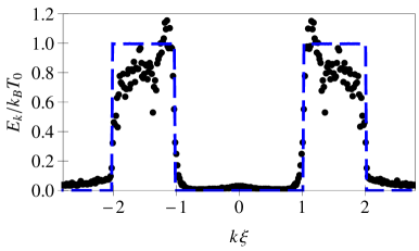
Figure 3: (Color online) Dots: mean energy per mode (scaled to $k_{\mathrm{B}}T_{0}$ with $k_{\mathrm{B}}T_{0}=0.66\,g\bar{n}$) as a function of wave number $k$ (scaled to $\xi$) for the dimensionless time $g\bar{n}t/\hbar=2\times 10^{4}$, which is long enough to provide equilibration. The Lieb-Liniger parameter $\gamma=5\times 10^{-3}$, $k_{1}\xi=1.0$, $k_{2}\xi=2.0$. Note the closeness of the equilibrium states to the initial energy distribution (dashed line).

We found that our method converges if the grid contains more than 200 points for $L\approx 400\,\xi$. A coarse grid (about 100 points) yields a numerical artifact: any initial distributions rapidly smears out to the “classical-like” flat distribution of the energy over modes, i.e. to $E_{k}\approx$  const for all momenta $-\frac{\pi}{\Delta x}<k<\frac{\pi}{\Delta x}$ resolvable by the grid with the step ${\Delta x}$.

To quantify relaxation of the system toward its equilibrium, we introduce the measure

$${W}=\frac{\sum_{k\neq 0}\left\{{\epsilon_{k}}[{\cal N}(k)-{\cal N}_{\mathrm{BE}}(k,T_{\mathrm{eq}})]\right\}^{2}}{\sum_{k\neq 0}[{\epsilon_{k}}{\cal N}_{\mathrm{BE}}(k,T_{\mathrm{eq}})]^{2}},$$ (5)

which has a meaning of the normalized energy-weighted squared deviation of the quasiparticle distribution from the Bose-Einstein thermal equilibrium. For the parameters of Figs. 1 and  2, with $T_{0}=150$ nK, the thermalization time is $\tau_{\mathrm{eq}}\sim 20$ ms. If we change $T_{0}$ to 50 nK and $k_{0}\xi$ to 1, then $\tau_{\mathrm{eq}}$ decreases by an order of magnitude. Note, that the obtained thermalization time $\tau_{\mathrm{eq}}$ is always shorter than the time needed for a sound wave to traverse the distance $L$. Therefore the thermalization observed in our simulations is a local physical effect, which is not related to specific boundary conditions. The thermalization time $\tau_{\mathrm{eq}}$ should not be confused with the time $\tau_{\mathrm{d}}\sim m\lambda_{\mathrm{T}}^{2}/\hbar$ Stim1 , where $\lambda_{T}=2\hbar^{2}\bar{n}/(mk_{\mathrm{B}}T)$, of dephasing between two 1D quasicondensates initially prepared in thermal-like states with strongly mutually correlated fluctuations.

III Discussion and conclusions

Therefore we found numerically an example of the GPE solution that relaxes toward a state with practically measurable noise and correlation properties DRBK well describable by a thermal Bose-Einstein ensemble of quasiparticles. As an illustration, in the inset in Fig. 2 we plot the numerically calculated first-order correlation function $g_{1}(x-x^{\prime})=\langle\Psi^{*}(x^{\prime},t)\Psi(x,t)\rangle/\bar{n}$ for $t=0$ and for $t$ large enough to provide equilibration prim3 . We see that this correlation function finally approaches the exponential form $g_{1}(x-x^{\prime})=\exp(-|x-x^{\prime}|/\lambda_{T})$, predicted for the thermal equilibrium Popov , with $T\approx T_{\mathrm{eq}}$ [the distance in the inset to Fig. 3 is scaled to $\lambda_{\mathrm{eq}}=2\hbar^{2}\bar{n}/(mk_{\mathrm{B}}T_{\mathrm{eq}})$].

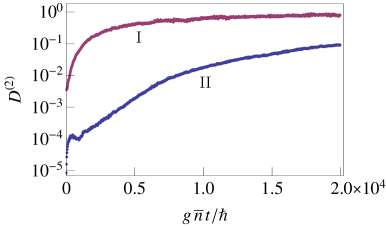
Figure 4: (color online) Distance $D^{(2)}[\psi_{1},\psi_{2}]$ (on the logarithmic scale, dimensionless) as a function of scaled time for the parameters of Fig. 1 (I, upper curve) and Fig. 3 (II, lower curve).

Not every initial distribution relaxes toward the Bose-Einstein thermal equilibrium. For example, if there are initially two oppositely propagating bunches of particle-like elementary excitations well separated in the momentum space, an equilibrium state very far from ${\cal N}_{\mathrm{BE}}(k,T_{\mathrm{eq}})$ is established, as seen from Fig. 3, where we assume $\epsilon_{k}{\cal N}_{0}(k)$ to be equal to $k_{\mathrm{B}}T_{0}$ for $k_{1}<|k|<k_{2}$ and zero otherwise ($k_{1}\gtrsim\xi^{-1}$). This behavior can be viewed as a conspicuous example of relaxation toward the fully constrained equilibrium Rigol1 in the weakly interacting case.

To elucidate the qualitative difference between the cases shown in Figs. 1 and 3, we calculate the time dependence of the distance $D^{(2)}[\psi_{1},\psi_{2}]=(2\bar{n}L)^{-1}\int_{0}^{L}dx\,|\psi_{1}(x,t)-\psi_{2}(x,t)|^{2}$ between two solutions $\psi_{1},\psi_{2}$ of the GPE, which are very close at $t=0$. As we can see from Fig. 4, if phononic modes are initially populated, $D^{(2)}$ grows exponentially and saturates at the unity level (corresponding to the total loss of correlations at $t\rightarrow\infty$), thus signifying the chaotic regime. If only particle-like modes are initially populated, then $D^{(2)}$ grows very slowly and stays well below 1 at all experimentally relevant times (hence, the chaotic behavior is practically not observed in that case).

To conclude, we numerically observed thermalization in a 1D quasicondensate, i.e. in an ultracold atomic system described by the NLSE with a cubic repulsive nonlinearity, if only phononic modes are populated initially. The correctness of the numerical solution has been checked via the criteria of the Lax operator isospectrality, conservation of the integrals of motion, and fidelity. Such a series of tests prevents the possible numerical artifacts that may occur in the split-step method s20 . Although the thermalization is not complete, experimentally measurable correlations are expected to be well described by the thermal equilibrium of bosonic elementary excitations. Our findings are in good agreement with the high efficiency of the evaporative cooling of ultracold atomic gases on the atom chips deeply in the 1D regime H1 ; H2 (our work on numerical modeling of evaporative cooling of ultracold bosonic atoms in elongated traps is in progress). On the other hand, to provide full thermalization of nonequilibrium ensembles of particle-like excitations, like the one displayed in Fig. 3, we have to resort to the option of the integrability breakdown provided by the mechanism of effective three-body elastic collisions in one dimension M089 .

This work was supported by the the FWF (Project No. P22590-N16). The authors thank J. Burgdörfer, N. J. Mauser, N. P. Proukakis, J. Schmiedmayer, and H.-P. Stimming for helpful discussions.

References

- (1) E. H. Lieb and W. Liniger, Phys. Rev. 130, 1605 (1963); E. H. Lieb, Phys. Rev. 130, 1616 (1963).
- (2) V.E. Zakharov and A.B. Shabat, Zh. Eksp. Theor. Fiz. 64, 1627 (1973) [Sov. Phys. JETP 37, 823 (1973)].
- (3) W. Eckhaus and A. van Harten, The Inverse Scattering Transform and the Theory of Solitons (North-Holland, Amsterdam, 1981); M. J. Ablowitz and P. A. Clarkson, Solitons, Nonlinear Evolution Equations and Inverse Scattering (Cambridge University Press, Cambridge, 1991).
- (4) S. Hofferberth, I. Lesanovsky, B. Fischer, T. Schumm, and J. Schmiedmayer, Nature (London) 449, 324 (2007).
- (5) S. Hofferberth, I. Lesanovsky, T. Schumm, A. Imambekov, V. Gritsev, E. Demler, and J. Schmiedmayer, Nature Phys. 4, 489 (2008).
- (6) I. E. Mazets, T. Schumm, and J. Schmiedmayer, Phys. Rev. Lett. 100, 210403 (2008); I. E. Mazets and J. Schmiedmayer, New J. Phys. 12, 055023 (2010); I.E. Mazets, Phys. Rev. A 83, 043625 (2011).
- (7) H.-P. Stimming, N. J. Mauser, J. Schmiedmayer, and I. E. Mazets, Phys. Rev. A 83, 023618 (2011).
- (8) B. Damski and W. H. Zurek, Phys. Rev. Lett. 104, 160404 (2010); E. Witkowska, P. Deuar, M. Gajda, and K. Rza̧żewski, Phys. Rev. Lett. 106, 135301 (2011).
- (9) S. P. Cockburn, D. Gallucci, and N. P. Proukakis, Phys. Rev. A 84, 023613 (2011).
- (10) I. Březinová, L. A. Collins, K. Ludwig, B. I. Schneider, and J. Burgdörfer, Phys. Rev. A 83, 043611 (2011).
- (11) N. P. Proukakis, J. Schmiedmayer, and H. T. C. Stoof, Phys. Rev. A 73, 053603 (2006).
- (12) A. Nunnenkamp, J. N. Milstein, and K. Burnett, Phys. Rev. A 75, 033604 (2007).
- (13) M. Rigol, V. Dunjko, V. Yurovsky, and M. Olshanii, Phys. Rev. Lett. 98, 050405 (2007).
- (14) M. J. Steel, .M. K. Olsen, L. I. Plimak, P. D. Drummond, S. M. Tan, M. J. Collett, D. F. Walls, and R. Graham, Phys. Rev. A 58, 4824 (1998); A. Sinatra, C. Lobo, and Y. Castin, J. Phys. B 35, 3599 (2002).
- (15) In our simulations we neglect the fluctuations of and always choose .
- (16) H.-P. Stimming, N. J. Mauser, J. Schmiedmayer, and I. E. Mazets, Phys. Rev. Lett. 105, 015301 (2010).
- (17) J. Armijo, T. Jacqmin, K. V. Kheruntsyan, and I. Bouchoule, Phys. Rev. Lett. 105, 230402 (2010).
- (18) is to be determined from Eq. (4) and not from since the total number of elementary excitations is not conserved.
- (19) M. Thalhammer, M. Caliari and C. Neuhauser, J. Comput. Phys. 228, 3 (2009).
- (20) S. Manz et al., Phys. Rev. A 81, 031610(R) (2010); T. Betz et al., Phys. Rev. Lett. 106, 020407 (2011).
- (21) The distribution of momenta of atoms (not to be confused with that of Bogoliubov quasiparticles) is given by the Fourier transform of .
- (22) V. N. Popov, Functional Integrals and Collective Excitations (Cambridge University Press, Cambridge, 1987); C. Mora and Y. Castin, Phys. Rev. A 67, 053615 (2003).
- (23) J. A. C. Weideman and B. M. Herbst, SIAM Journal on Numerical Analysis 23, 485 (1986); T. I. Lakoba, Numer. Methods Partial Differ. Equations (2010).