Asymmetric Double Quantum Wells with Smoothed Interfaces

Abstract

We have derived and analyzed the wavefunctions and energy states for an asymmetric double quantum wells, broadened due to static interface disorder effects, within well known discreet variable representation approach for solving the one-dimensional Schrodinger equation. The main advantage of this approach is that it yields the energy eigenvalues and the eigenvectors in semiconductor nanostructures of different shapes as well as the strengths of the optical transitions between them. We have found that interface broadening effects change and shift energy levels to higher energies, but the resonant conditions near an energy coupling regions do not strongly distorted. A quantum-mechanical calculations based on the convolution method (smoothing procedure) of the influence of disorder on the motion of free particles in nanostructures is presented.

I Introduction

When a thin ($\sim$100 A) layers of one semiconductor (e.g. GaAs) are sandwiched between layers of another semiconductor with a larger bandgap (e.g. AlGaAs), carriers are trapped and confined in two dimensions (2D), due to the potential barriers. As a result of quantum confinement discrete energy states (or ”subbands”) occur, which change dramatically electronic and optical properties of such structures, called as the quantum wells (QWs). When the quantum wells are coupled there exist probabilities for the electron tunnel and be in either of the two wells. The novel optical properties of the 2D electron gas, associated with the transitions between quantized subbands, so called ”intersubband transitions”, correspond from mid-infrared to terahertz (THz) photon energies. They have narrow line-widths and extremely large transition dipole moments.

In recent years, there has been considerable interest in asymmetrical multiple-quantum well systems, because many new optical devices based on intersubband transitions are being developed. This feature could fulfill the need for efficient sources of coherent infrared (IR) radiation for several applications, such as communications, radar, and optoelectronics. Their most spectacular applications are quantum well IR photodetectors [1] and the quantum cascade (QC) lasers [2] that relies on the intersubband transitions and resonant tunneling between adjacent QWs. Moreover, intersubband transitions give rise to extremely high linear and nonlinear optical susceptibilities. Specially engineered asymmetric quantum wells possess resonant 2^nd and 3^rd order optical nonlinearities which are respectively 3 and 5 orders of magnitude higher than that in the bulk semiconductors, which may be used for frequency mixing, phase conjugation and all-optical modulation [3]. These devices are made with epitaxially grown GaAs/AlGaAs and InGaAs/AlInAs [4]. With the recent development on semiconductor devices growth by the molecular beam epitaxy and metal-organic chemical vapor deposition techniques, multi-barrier quantum well structures are becoming the basic building blocks of modern semiconductor devices, such as resonant tunneling diodes (RTD) [5], far-infrared and THz lasers [6], quantum cascade (QC) lasers [2,7], etc.

Real QW structures tend to deviate from the ideal homogeneous heterostructure with perfectly smooth interfaces. The reasons are the stochastic processes of the crystal growth leading to local variations of chemical composition, well width, and lattice imperfections to name a few. Since a QW is generally a heterostructure formed by a binary semiconductor (AB) and a ternary disordered alloy (AB_1-xC${}_{x})$, as in InGaAs/GaAs, there are two types of disorders responsible for the inhomogeneous broadening: compositional disorder caused by concentration fluctuations in a ternary component and random diffusion across the interface. In order to design new devices or optimize the device performance, and thus properly predict their behavior, one needs to know the detailed information of quasi-bound levels in real disordered multi-barrier quantum well structures. Theoretical studies of effects due to compositional and interface disorders have a long history [8-10].

To understand the physical properties of the heterostructure devices, one needs to solve the eigenvalue problem of carriers in QWs. It is well known that exact analytic solutions to such problems are only available for simple structures such as square or parabolic well [11] and even in these structures, in general, in the presence of perturbations such as external fields, disorder effects [12], etc. the problem cannot be solved exactly.

There have been various numerical methods used to calculate the band profiles in QWs: the matrix approach (MA) [13], the transfer matrix (TM) method [14, 15], the finite difference method (FDM) [16, 17], the finite element (FE) technique [18, 19], discreet variable representation (DVR) approach [20], envelope function (EF) method [21], Wentzel–Kramers–Brillouin (WKB) approximation [22], variational method (VM) [23], and Monte Carlo (MC) simulations [24]. Among them, the WKB and EF methods adopt approximations, thus give the results unreliable; the VM only works well at simple QWs and weak fields; the MC and FE methods are highly computer-orientated approaches; the MA usually require wave function to be well behaved. While DVR as also TM methods overcomes all the shortcomings listed above and could be easily applied to any potential profiles of biased/unbiased multi-barrier quantum well structures.

In this paper we describe shortly a numerical technique based on the DVR approach, as a grid-point representation of a Hamiltonian matrix elements [12, 20, 25], which is capable of solving the eigenvalue and eigenfunction problems in an arbitrary QWs under arbitrary perturbation, for an asymmetric double quantum wells with interfaces broadened due to static disorder effects.

II Calculation details

II.1 A model of the interface disorder effects

Randomly distributed charged dopants, or composition x in mixed crystals A_xB_1-x, lead to unavoidable fluctuations of the doping impurities concentration on a microscopic scale. Two things influence as an interface disorder effects: coordinate fluctuations of interface position (Fig 1 a), and gap energy E_g(x) fluctuations (Fig 1 b,c) due to the randomly distributed dopants. These fluctuations result in potential fluctuations. This situation is schematically shown in Fig 1. The magnitude of band-edge energy fluctuations (Fig 1 b,c) caused by the random distribution of charged donors and acceptors was first calculated by Kane [26]. States with energy below the unperturbed conduction band edge or above the unperturbed valence band edge are called tail states, which significantly change the density of states in the vicinity of the band edge. The absence of order means that the wavevector k is no longer a good quantum number. At energies high in the band this spread in k values can be described by a mean free path, but deep in the tail localization is complete.

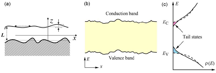
Figure 1: (a) Characteristic length scales describing the interface roughness of a QW. (b) Spatially locally fluctuating band edges caused by random distribution of impurities (internal Franz-Keldysh effect), after [27]. (c) Resulting densities of states in the conduction with tail states extending into the forbidden gap. The dashed lines show the parabolic densities of states in undoped semiconductors.

Particularly simple models of an electron moving in a random potential are possible. If the fluctuations are not too large, good approximation is obtained by calculating spectra for slightly different configurations and adding them up using some broadening weight factor. Inhomogeneous broadening, due to site variation produced by a random distribution of local crystal fields, results in a Gaussian type broadening [26]. Homogeneous broadening, from dynamic perturbations on energy levels and equally on all ions, leads to a Lorentzian type broadening. So, QW’s barrier interface roughness may be approximated [12] by the convolution of Heaviside step function $\Phi$(x-x${}_{0})$ with an area normalized, moving Gaussian broadening envelope function of width $\sigma_{G}$:

$$H_{G}(z,z_{0},\sigma)=\frac{1}{\sqrt{2\pi}\sigma_{G}}\int\limits_{0}^{\infty}{\exp\left[{-\frac{(z-x)^{2}}{2\sigma_{G}^{2}}}\right]}\,\Phi(x-z_{0})dx,$$ (1)

or with the Lorentzian broadening envelope function of width $\Gamma$:

$$H_{L}(z,z_{0},\Gamma)=\frac{\Gamma}{\pi}\int\limits_{0}^{\infty}{\frac{1}{(z-x)^{2}+\Gamma^{2}}\,}\Phi(x-z_{0})dx.$$ (2)

A convolution (smoothing) procedure [28] is an integral that expresses the amount of overlap of envelope function (i.e. Gaussian or Lorentzian) as it is shifted over another function $\Phi$. Instead of the $\infty$ limit in integrations usually is used any enough big value for the result convergation. The barrier steps may be broadened also in extremely simple analytical way, - by applying of the phenomenological atan(x) function against the Heaviside step function $\Phi$(x), usual for an ideal heterostructure with perfect interfaces:

$$\Phi(z-z_{i})\Rightarrow\frac{\pi}{2}+\arctan\frac{z-z_{i}}{\Gamma_{i}}$$ (3)

where $\Gamma_{i}$ is broadening parameter of the interfaces at z_i. This function with zero mean z_i, characterize the deviation of the i^th interface from its average position. Examples of calculated functions (1)-(3) are presented in Fig 2. As we see in Fig 2, this function (3) (red dots) may be a good approximation for convolution of Heaviside function by Lorentzian envelope (2) (curve 3).

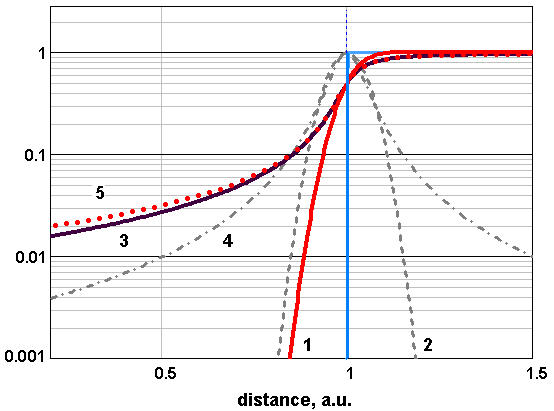
Figure 2: Comparison of convolution broadenings of the Heaviside step-function with different broadening functions: 1 – Gaussian broadened step (1); 2 – Gaussian envelope; 3 – Lorentzian broadened step (2); 4 - Lorentzian envelope; 5 – Analytical arctan(x) approximation curve (3). Broadening parameter $\Gamma$ = 0.05 nm.

II.2 Method of Discrete Variable Representation (DVR)

Analytical expressions for asymmetrical double and triple quantum-wells are possible only for idealized rectangle QWs [29]. We select discrete variable representation (DVR) as a numerical method [20, 30] for our MathCAD calculations of stationary 1D Schrodinger equation for confined eigenstates. Different types of DVR methods have found wide applications in different fields of problems [31, 32]. We also carried out DVR calculations for QWs an unharmonic Morse potential [12, 25].

The DVR is a numerical grid-point method in which the matrix elements of the local potential energy operator V(r) is approximated as a diagonal matrix (mnemonic: DVR - diagonal V(r), or Discrete Variable Representation): V_ik = $\langle\phi_{i}|$V$|\phi_{k}\rangle=\delta_{ik}$V(x${}_{i})$ [31], and the kinetic energy matrix is full, but it has simple analytic form, as a sum of 1D matrices. DVR method is selected since it avoid having to evaluate integrals in order to obtain the Hamiltonian matrix and since an energy truncation procedure allows the DVR grid points to be adapted naturally to the shape of any given potential energy surface. The DVR method greatly simplifies the evaluation of Hamiltonian matrix elements H_ik = $\langle\phi_{i}|$H$|\phi_{k}\rangle$ and obtains the eigenstates and eigenvalues by using standard numerical diagonalization methods of MathCAD or Mathematica.

If we choose an equally spaced grid, x_i = i$\Delta$x, (i = 0, $\pm$1, $\pm$2, … $\pm$N), then the DVR gives an extremely simple grid-point representation of the kinetic energy matrix $\hat{T}_{i,k}={\hbar^{2}k_{i,k}^{2}}\mathord{\left/{\vphantom{{\hbar^{2}k_{i,k}^{2}}{2m^{\ast}}}}\right.\kern-1.2pt}{2m^{\ast}}$ within the conditional formulation [20]:

$$\mathord{\buildrel\lower 3.0pt\hbox{$\scriptscriptstyle\frown$}\over{T}}_{i,k}=g\,\left\{{{\begin{array}[]{*{20}c}{{\,\,\pi^{2}}\mathord{\left/{\vphantom{{\,\,\pi^{2}}3}}\right.\kern-1.2pt}3,{\begin{array}[]{*{20}c}\hfill\hfil&\hfill\hfil\\ \end{array}\hfill}}&{i=k\hfill}\\ {\frac{2\,(-1)^{i-k}}{(i-k)^{2}},\hfill}&{i\neq k\hfill}\\ \end{array}}}\right\}.$$ (4)

The only parameter involved being the grid spacing $\Delta$x via an energetically weighted grid parameter g (“energy quantum of the grid”):

$$g=\frac{\hbar^{2}}{2m^{\ast}}\left({\frac{1}{\Delta x}}\right)^{2}$$ (5)

where m^∗ is the electron effective mass. So, if the grid points are uniformly spaced then numerical solutions of a matrix elements of the full energy Hamiltonian operator

$$\hat{H}=\mathord{\buildrel\lower 3.0pt\hbox{$\scriptscriptstyle\frown$}\over{T}}+\hat{V}=-\frac{\hbar^{2}}{2m^{\ast}}\frac{d^{2}}{dx^{2}}+V(x)\,$$

is as [20]:

$$\hat{H}_{i,k}=\mathord{\buildrel\lower 3.0pt\hbox{$\scriptscriptstyle\frown$}\over{T}}_{i,k}+\hat{V}_{i,k}=\frac{\hbar^{2}}{2m(\Delta x)^{2}}(-1)^{i-k}\left({\frac{\pi^{2}}{3}\delta_{i,k}+\frac{2\,}{(i-k)^{2}}(1-\delta_{i,k})}\right)\,+V(x_{i})\,\delta_{i,k}$$ (6)

when the $\delta$-functions are placed on a grid that extends over the interval x = (-$\infty$,$\infty)$. First term in parenthesis is a value of second term in the limit N $\to$ $\infty$ [20].

In our calculations the potentials of an ideal and of a broadened double QW are used as [12]:

$$V_{1}(x_{i})=U_{1}\,[\,1-\Phi(x_{i}+R_{1})+\Phi(x_{i}-R_{1})],$$

$$V_{2}(x_{i})=V_{1}(x_{i})+U_{2}\,[\,\Phi[x_{i}-(R_{b}+R_{2})]-\Phi(x_{i}-R)],$$ (7)

and

$$V_{1}(x_{i})=U_{1}\,[\,1+\frac{1}{\pi}\arctan{\kern 1.0pt}\left({\frac{x_{i}}{\Gamma}}\right)-\frac{1}{\pi}\arctan{\kern 1.0pt}\left({\frac{x_{i}+R_{1}}{\Gamma}}\right)],$$

$$V_{2}(x_{i})=V_{1}(x_{i})+U_{2}\,[\,\frac{1}{\pi}\arctan{\kern 1.0pt}\left({\frac{x_{i}-(R_{b}+R_{2})}{\Gamma}}\right)-\frac{1}{\pi}\arctan{\kern 1.0pt}\left({\frac{x_{i}-R_{b}}{\Gamma}}\right)],$$ (8)

correspondingly. Here $\Phi$(x) is a Heaviside step function; U₁₍₂₎ are the depths of potential wells (differences in the offset band energies) for the 1^st and 2^nd QW of the widths R₁₍₂₎; and R_b is the barrier width. One can reasonably argue the restriction of used approximation for QWs disorder effects via an effective potentials (8). Arguments may be directed to the problem being subject to short-range energy fluctuations which may be treated as a “white-noise” disorder with small correlation lengths.

III Results and discussion

Inter-well optical-phonon-assisted transitions are studied in an asymmetric double-quantum-well heterostructures [33] comprising one narrow and one wide coupled quantum wells (QWs). It is shown that the depopulation rate of the lower subband states in the narrow QW can be significantly enhanced thus facilitating the intersubband inverse population, if the depopulated subband is aligned with the second subband of the wider QW, while the energy separation from the first subband is tuned to the energy of optical phonon mode.

Seeking to reproduce mentioned effects of [33], the eigenvalues (stationary energy states E${}_{n})$ and the eigenvectors (wavefunctions $\psi_{n})$ for a quantum number $n$, as the solutions of the Schrodinger equation $\hat{H}\psi_{n}(r)=E_{n}\psi_{n}(r)$, were calculated using standard numerical diagonalization methods (eigenvals(H) and eigenvec(H) commands in MathCAD) for the DVR Hamiltonian (6).

Results of our DVR calculations of such a laser structure as in [33] are depicted in Fig 3 as the eigenstates together with the corresponding wavefunctions for the coupled asymmetric square quantum wells with the potentials of the form (7). The states over the dissociation energy U are unbound and delocalized. Dependencies of the positions of the five lowest subbands B_i as a function of the narrow well width values R₁ = 3, 5, 7, 10, 12, 15 nm for the fixed values of barrier width R_b = 2 nm and of the second QW width R₂ = 15 nm are shown in Fig 3. Broken lines are the same dependencies for the A_i states of a 1^st, but single, quantum well with the same width R₁. Comparing the fans of dependencies for A_i and B_i states for single and double QW’s, we can resolve the doublet nature of the states and especial coupling (anti-crossing) regions of the levels in double QW. The insets around in Fig 3 show the model band diagrams with energy levels and corresponding wavefunctions of an ADQW heterostructures (AlAs/GaAs). It is useful also to have some indication of how many grid points are necessary for this DVR to provide an accurate description of a quantum system. Convergence of the calculation can be checked by decreasing the number of grid used in calculation. For full convergence of the calculation results we found that enough number of grid is N $\geq$ 50, however we have used the number of calculus points N = 500 for the better shaping of calculated wavefunctions.

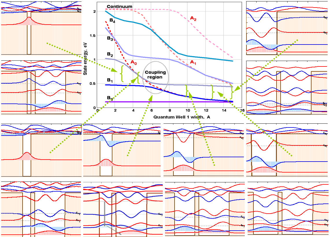
Figure 3: Unbroadened ideal ADQWs case. Dependencies of the positions of the five lowest subbands B₀ – B₄ (in eV) as a function of the narrower well width R₁ (= 3, 5, 7, 10, 12, 15 nm) for fixed values R_b = 2 nm and R₂ = 15 nm. Broken lines are the same dependencies of the A states for a single quantum well of R₁ width. The insets around show the model band diagrams with energy levels and corresponding wavefunctions of an asymmetric double quantum well heterostructures. Double-lined arrow corresponds to the stimulating light-emitting transition, assisted by the resonant phonon emission (arrow between states n=1 and n=0) in the heterostructure. Calculated region: -30 nm $\div$ +30 nm with 500 grids.

All states in double QW are splitted doublets, because the degeneracy is unmounted by different parity properties. When the barrier thickness becomes smaller, quantum coupling due to the tunneling between the wells has the place. As a consequence, an energy splitting occurs (rounded regions indicated in Fig 3 and Fig 4) and the respective electron states, the so-called binding and anti-binding states, are delocalized over both wells. The energy splitting or tunnel coupling $\Delta$E is determined by the barrier thickness R_b and height. The resonant situation can be obtained for asymmetric, coupled double quantum wells with applied bias [33]. The lowest coupled state is mainly localized in the wide well and the other state is mainly localized in the narrow well. Due to the coupling of the two wells the two states have nonzero probability density in both wells. Under a suitable bias these two states become resonant.

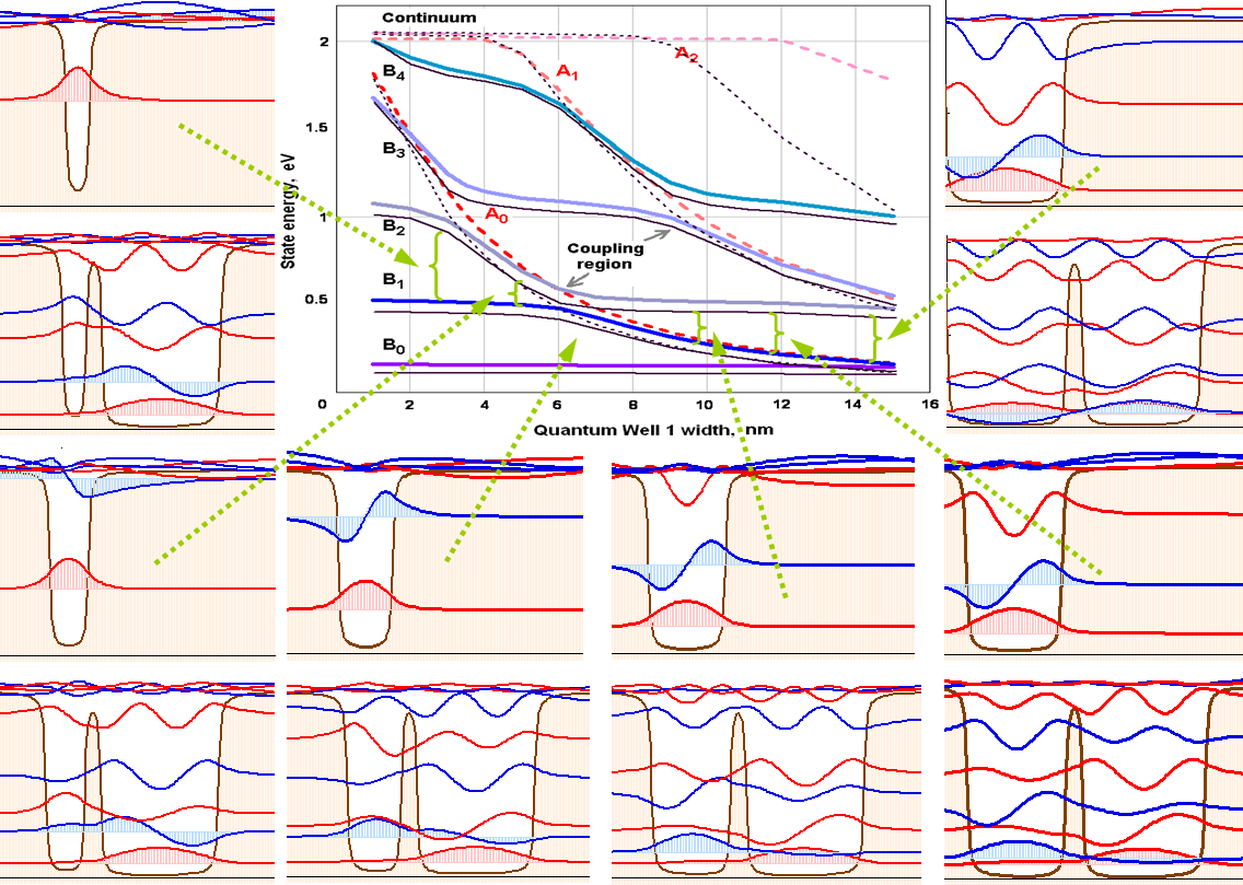
Figure 4: Broadened ADQWs case. Dependencies of the positions of the five lowest subbands B₀ – B₄ (in eV) as a function of the narrower well width R₁ (= 3, 5, 7, 10, 12, 15 nm) for fixed values R_b = 2 nm and R₂ = 15 nm. Broken lines are the same dependencies of the three A_i states for a single QW with the width R₁. For comparison, thin black lines presents the case of ideally rectangle shaped ADQWs as in Fig 3. The insets around shows the model band diagrams with energy levels and corresponding wavefunctions. Interface roughness parameter $\Gamma$ = 0.2 nm. Calculated region: -30 nm $\div$ +30 nm with 500 grids.

One embodiment of THz laser structure is depicted in Fig 3 and Fig 4 where the energy levels in coupling region are separated by energy equal to the optical phonon energy. Double-lined arrow corresponds to the stimulated light-emitting transition, assisted by the resonant phonon emission (arrow between states n=1 and n=0). Phonon-assisted transitions between the coupled levels depend strongly on the phonon energy involved in the transition.

The results of DVR calculations of the same family of ADQWs as in Fig 3, but with structurally broadened interfaces with the potentials approximated by (8), with used interface roughness parameter $\Gamma$ = 0.2 nm, are depicted in Fig 4. In the central part of Fig 4 both energy fans for an ideal rectangular interfaces (as in Fig 3) and for a broadened ones are presented together and mutually compared. Here the thin black lines presents the case of ideally rectangle shaped ADQWs. As we see, interface broadening change and shift energy levels to the higher energies, but the resonant conditions near an energy coupling regions do not strongly distorted. The blue shift is as a sequence of an effective narrowing of the distorted QWs, but the changes seen in the coupling regions are caused from the different inter-well barrier profile.

IV Conclusions

The discreet variable representation approach for solving the one-dimensional Schr dinger equation is performed to calculate the structural and electronic properties of asymmetric double quantum wells broadened due to static interface disorder effects. We have derived and analyzed the wave functions, and the energy states for the structurally disordered (broadened) quantum wells of different profiles. The interlayer interactions would destroy the state degeneracy, induce more states, and vary their energy. Interface broadening effects change and shift energy levels to higher energies, but the resonant conditions near an energy coupling regions do not strongly distorted.

References

- (1) B. Levine, et al., Appl. Phys. Lett. 50, 1092 (1987)
- (2) J. Faist, F. Capasso, D. L. Sivco, C. Sirtori, A. L. Hutchinson, A. Y. Cho, Science 264, 553 (1994)
- (3) K. Vodopyanov, et al., Appl. Phys. Lett. 72, 2654 (1998)
- (4) J. Faist, F. Capasso, C. Sirtori, D. L. Sivco, A. Hutchinson, A. Cho, Appl. Phys. Lett. 67, 3057 (1995)
- (5) T. Sollner, W. Goodhue, P. Tannenwald, C. Parker, Appl. Phys. Lett. 43, 588 (1983)
- (6) R. K hler, et al., Nature 417, 156 (2002)
- (7) J. S. Yu, A. Evans, J. David, L. Doris, S. Slivken, M. Razeghi, IEEE Photonics Technol. Lett., 16, 747 (2004)
- (8) A. Efros, and M. Raikh, in Optical Properties of Mixed Crystals, R. Elliott, I. Ipatova (Ed.) (North-Holland, Amsterdam, 1988), p. 133
- (9) M. Herman, D. Bimberg, J. Christen, J. Appl. Phys. 70, R1 (1991)
- (10) E. Runge, Solid State Physics, H. Ehrenreich, F. Spaepen (Ed.) (Academic, San Diego, 2002)
- (11) H. Wang, H. Xu, and Y. Zhang, Phys. Lett. A 340, 347 (2005)
- (12) V. Gavryushin, SPIE Proc. 6596, 659619 (2007)
- (13) A. K. Ghatak, K. Thyagarajan, M. R. Shenoy, Thin Solid Films, 163, 461 (1988); IEEE J. Quant. Electron. 24, 1524 (1988)
- (14) E. Anemogiannis, E. N. Glysis, T. F. Gaylord, T. K. Gaylord, IEEE J. Quant. Electron. 29, 2731 (1993)
- (15) E. P. Samuel, D. S. Patil, Progress in Electromagnetics Research Lett., 1, 119 (2008)
- (16) P. Harrison, Quantum wells, wires and dots: Theoretical and computational physics, 2nd ed., Wiley, Chichester, UK, 2005
- (17) B. M. Stupovski, J. V. Crnjanski, D. M. Gvozdi , Comput. Phys. Commun. 182, 289 (2011)
- (18) K. Nakamura, A. Shimizu, M. Koshiba, K. Hayata, IEEE J. Quant. Electron. 25, 889 (1989)
- (19) Khai Q. Le, Microwave and Optical Technology Lett. 51, 1 (2009)
- (20) D. Colbert, W. Miller, J. Chem. Phys. 96, 1982 (1992)
- (21) E. J. Austin, M. Jaros, Phys. Rev. B 31, 5569 (1985)
- (22) J. Heremans, D. L. Partin, P. D. Dresselhaus, Appl. Phys. Lett. 48, 644 (1986)
- (23) D. Ahn, S. L. Chuang, Appl. Phys. Lett. 49, 1450 (1986)
- (24) J. Singh, Appl. Phys. Lett. 48, 434 (1986)
- (25) V. Gavryushin, arXiv:q-bio/0510041v1 [q-bio.BM]
- (26) E. O. Kane, Phys. Rev. 131, 79 (1963)
- (27) J. I. Pankove, Optical Processes in Semiconductors, Dover Publications Inc., New York, 1975
- (28) E. W. Weisstein, ”Convolution.” Wolfram Web Resource. http://mathworld.wolfram.com/Convolution.html
- (29) R. Betancourt-Riera, R. Rosas, I. Marzn-Enriquez, R. Riera, J. L. Marin, J. Phys. C. 17, 4451 (2005)
- (30) G. W. Wei, J. Phys. B. 33, 343 (2000)
- (31) H. S. Lee, J. Light, J. Chem. Phys. 120, 4626 (2004)
- (32) J. Tennyson, et al., Comput. Phys. Commun. 163, 85 (2004)
- (33) M. A. Stroscio, M. Kisin, G. Belenky, S. Luryi, Appl. Phys. Lett. 75, 3258 (1999)