High angular resolution imaging with stellar intensity interferometry using air Cherenkov telescope arrays
Abstract
Optical stellar intensity interferometry with air Cherenkov telescope arrays, composed of nearly 100 telescopes, will provide means to measure fundamental stellar parameters and also open the possibility of model-independent imaging. In addition to sensitivity issues, a main limitation of image recovery in intensity interferometry is the loss of phase of the complex degree of coherence during the measurement process. Nevertheless, several model-independent phase reconstruction techniques have been developed. Here we implement a Cauchy-Riemann based algorithm to recover images from simulated data. For bright stars () and exposure times of a few hours, we find that scale features such as diameters, oblateness and overall shapes are reconstructed with uncertainties of a few percent. More complex images are also well reconstructed with high degrees of correlation with the pristine image. Results are further improved by using a forward algorithm.
keywords:
techniques: high angular resolution - instrumentation: interferometers - stars: imaging - stars: fundamental parameters1 Introduction
Even though Stellar Intensity Interferometry (SII) was abandoned in the 1970’s,
there has been a recent interest in reviving this technique, mainly due to the
unprecedented plane coverage that future imaging air Cherenkov telescope (IACT) arrays will
provide (CTA Consortium, 2010; , 2009). The possibility of probing stars at the
sub-milliarcsecond scale and visible wavelengths has motivated new developments in instrumentation and
simulations, the latter being the focus of this paper.
Recent results obtained with amplitude (Michelson) interferometry have started to
reveal stars as extended objects (e.g. Baldwin et al. 1996; 2007), and with non-uniform light
intensity distributions in the milliarcsecond scale.
Such interesting results can be further investigated with SII taking advantage of the longer (km)
baselines and relative ease of observing at shorter (blue) wavelengths.
For example, measuring stellar diameters at different wavelengths, will make it possible to further investigate the
wavelength dependence of limb darkening,
(, 2003) and thus constrain stellar atmosphere models. Radii measurements with uncertainties of a few percent, along
with spectroscopic measurements are necessary
to constrain the position of stars in the HR diagram (e.g. 2008). With the
methods described in this paper, we show that diameters can in principle be measured
with accuracies better than when using realistic array
configurations for future experiments such as CTA (Cherenkov Telescope
Array). As another example we can consider
fast rotating B stars, which are ideal candidates for imaging oblateness,
pole brightening (, 2007, 1924), radiatively driven mass loss (, 1986), and perhaps even pulsation modes
(, 2006). The impact of rotation on stellar evolution is non-trivial, and
several studies have been made in the subject (e.g. 1996, 1997). Images of rotating stars have become available
in the past few years (e.g. Monnier et al. 2007; Aufdenberg et al. 2006), and
measurements of oblateness with accuracies of a few percent have been made.
We will show that this is comparable to what
can be achieved with SII using large arrays of Cherenkov telescopes.
There is also the case of interacting binaries, for which we can measure angular separation,
diameters, and relative brightness. It may even be possible to measure mass transfer (, 2007). Measurements of the angular separation
in binaries is crucial for determining the masses of stars. These masses must be found to within (, 1991)
in order to test main sequence models. With the methods described in this paper, we show that angular
separations can be found to within a few percent from reconstructed images. A more convenient and
accurate analysis (beyond the scope of this paper) does not require imaging, and should yield sub-percent uncertainties,
so that testing main sequence models will become possible with SII.
In preparation for a large-scale SII observatory deployment, several
laboratory experiments are in progress (, 2010). Their main goal is to measure light intensity correlation between two receivers.
It is also worth mentioning the Star Base observatory
(located in Grantsville, Utah) which consists of two light receivers separated by and which will be used
to test high time resolution digital correlators,
and to measure the second order degree of coherence for a few stars. Various analog and digital correlator
technologies (, 1994) are being implemented, and cross correlation of streams of photons with
nanosecond-scale resolution has already been achieved.
Intensity interferometry, unlike amplitude interferometry, relies on the correlation between intensity fluctuations averaged over the spectral band at electronic (nanosecond) time resolution. These averaged fluctuations are much slower than the (femtosecond) light wave period. This correlation is directly related to the complex degree of coherence as (, 2006)
| (1) |
Here, is the time average of the intensity received at a particular
telescope , and is the intensity fluctuation. Measuring
a second-order effect results in lower signal-to-noise ratio when compared to amplitude interferometry (, 2006). This
sensitivity issue can be dealt with by using large light collection areas
(such as those available with air Cherenkov telescopes), longer exposure times
and baseline redundancy.
The low frequency fluctuation can be interpreted classically as the beat formed by
neighboring Fourier components.
Since SII relies on low frequency
fluctuations, which are typically several orders of magnitude smaller than the
frequency of optical light, it does not rely on the phase difference between light waves,
but rather in the difference between the relative phases of the two components
at the detectors (, 1974). The main advantage is the relative insensitivity to
atmospheric turbulence and the absence of a requirement for sub-wavelength precision
in the optics and delay lines (, 1974).
The complex mutual degree of coherence is proportional to the Fourier
transform of the radiance distribution of the object in the sky (Van Cittert-Zernike theorem).
However, since with SII, the
squared-modulus of is the measurable quantity, the main
disadvantage is that the phase of the Fourier transform is lost in the
measurement process. The loss of phase information poses a severe difficulty,
and images have in the past been reconstructed from the bispectrum technique,
using monolithic apertures (e.g. Lawrence et al. 1990).
The imaging limitations
can be overcome using a model-independent phase recovery technique. Even though
several phase reconstruction techniques exist (Fienup, 1981), we concentrate on a two
dimensional version of the one dimensional analysis introduced by (2004), which is based on the theory of analytic functions,
and in particular the Cauchy-Riemann equations.
Following recent successes in Gamma ray astronomy, a next generation Cherenkov telescope array is in a preparatory stage. This project is currently known as CTA (Cherenkov telescope array) (CTA Consortium, 2010), and will contain between 50 and 100 telescopes with apertures ranging between and . In this paper we investigate the sensitivity and imaging capabilities of SII implemented on such an atmospheric Cherenkov telescope array. We start with a discussion of sensitivity (section 2), followed by a discussion of simulating noisy data as would be realistically obtained with such an array (section 3). Since data have a finite sampling in the plane, we discuss our method of fitting an analytic function to the data in order to estimate derivatives which are needed for phase reconstruction (section 4). We then briefly discuss phase recovery (section 5) and proceed to quantify the reconstruction quality using several criteria. We start with the simple case of uniform disks (section 6.1) and progressively increase the degree of image complexity by including oblateness (section 6.2), binary stars (section 6.3), and obscuring disks and spots (section 6.4).
2 Sensitivity
The signal to noise ratio (SNR) for an intensity correlation measurement depends on the degree of correlation , the area of each of the light receivers, the spectral density (number of photons per unit area per unit time, per frequency), the quantum efficiency , the electronic bandwidth , and the observation time . The SNR can be expressed as (, 1974)
| (2) |
The spectral density is related to the visual magnitude of the star as well as its temperature
and observing wavelength . The spectral density is the number of black body photons
per unit area, per unit frequency and per unit time. The dependence of the visual magnitude is found by
recalling that the flux for a magnitude star with a temperature of observed at
is (Bessell, 1979). This in turn corresponds to a spectral density of
. The
spectral density as a function of temperature (for different visual
magnitudes and observing wavelengths) is shown in Fig. 1, and we see that at constant visual magnitude
and observing wavelength, higher temperatures correspond to higher spectral densities. We find that the increase
in temperature is approximately for the
range of temperatures and wavelengths considered in Fig. 1. For example, at , a decrease of 1 visual
magnitude is equivalent to increasing the temperature of the star from to . For
this reason high temperature objects are easier targets for SII.

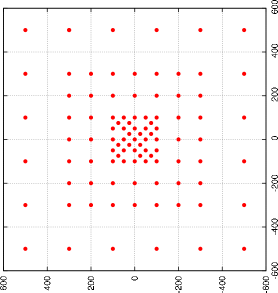
We use a preliminary design of the CTA project as an array configuration (Bernlöhr, 2008), which is shown in
Fig. 2. This array contains
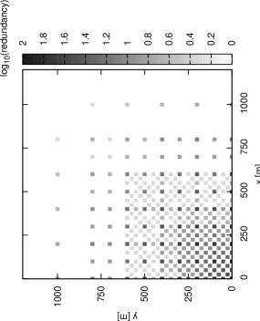
telescopes and baselines (many of which are redundant) which are shown in Fig. 3. Each detector is
assumed to have a light collecting area of and a
light detection quantum efficiency of . Using a criterion, we find that
the largest baselines of resolve angular
scales of at .
The smallest baselines of resolve angular scales
of . However, we show in section 6.1,
that the largest angular scales that can be realistically imaged with our analysis,
in a model independent way, are more determined by
baselines of . This is because the estimation
of derivatives of the phase (needed for phase recovery) degrades as the number of
baselines is reduced. Baselines of resolve
angular scales of at .
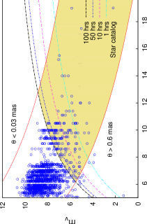
These order-of-magnitude considerations are taken into account when performing simulations and image reconstructions, i.e. the minimum and maximum size of pristine images that can be reconstructed by data analysis, do not go far beyond these limits. More precise array resolution limits are presented in section 6.1 (diameters ranging between ) . By combining these angular scales with the SNR (eq. 2), we obtain Fig. 4. This figure shows the highest visual magnitude, for which photon correlations (with ) can be detected (5 standard deviations), as a function of the temperature, and for several different exposure times. Also shown in Fig. 4, is the shaded region corresponding to angular diameters between and 111These curves of constant angular size can be found approximately by recalling that the visual magnitude is related to a calibrator star of visual magnitude by: . Here, and refer to the flux in the visual band . To express as a function of the angular size, note that flux is proportional to , where is the angular size and is the temperature of the star., and observable within . From the Figure we can see how correlations of photons from faint stars can be more easily detected if they are hot. To quantify the number of stars for which photon correlations can be detected with the IACT array, we perform use the JMMC stellar diameters catalog (Lafrasse et al., 2010). We find that (out of ) stars from the JMMC catalog can be detected within , correlations from stars can be detected within , and can be detected within . In Fig. 2, we show a random sample of 2000 stars (out of ) from the JMMC catalog. Interstellar reddening may play a role in reducing the number of measurable targets
3 Simulation of realistic data
The original “pristine” image consists of
pixels corresponding to of angular extension and a
wavelength of . The
Fourier transform of the image is then performed via an FFT algorithm and
normalized so that its value is one at zero baseline. This results in a
Fourier transform sampled every ,
i.e. cycles per radian field-of-view at a wavelength of . We then find
the squared-modulus of the degree of coherence between the members of each pair of telescopes.
This is obtained from a linear interpolation of the squared Fourier magnitude in the finely
sampled FFT. Diurnal motion is not taken into account in the simulations. Diurnal motion plays
a significant role in increasing the coverage when exposure times are long.
As a consequence there is less coverage in the simulations since
projected baselines do not drift with time. The smaller
coverage is however compensated by smaller statistical error in the correlation measurements.
The final step in the simulation phase is the addition of noise to the
correlation at each baseline. This noise was found to be
Gaussian by performing the time integrated product of two random streams of
simulated photons as detected by a pair of photo-multiplier tubes. The standard
deviation of the noise added to each pair of telescopes is calculated
from eq. 2. In this paper we take the signal bandwidth to be . An example of simulated data as a function of telescope separation
is shown in Fig. 5. This corresponds to a magnitude
uniform disk star () of radius
and of observation time. The software used for the simulations, as well as the
analysis222See sections 4 and 5 for details on the analysis. Some
variants of the analysis software were developed in MATLAB. All software is available upon request., was developed in C.

4 Fitting an Analytic function to the data
The estimation of derivatives of the Fourier log-magnitude is at the heart of the Cauchy-Riemann phase
recovery algorithm (section 5), and is thus greatly simplified when data is known on
a square grid rather than in a ‘randomly’ sampled way as is directly available
from observations. Once simulated data are available (or observations in the future), an analytic function is fitted to
the data.
An analytic function can be expressed as a linear combination of basis functions. When data are available at baselines , with uncertainty , the coefficients of the basis functions can be found by minimizing the following :
| (3) |
Each is the coefficient of a basis function . The constant is a scaling factor,
and is a rotation operator. The scaling factor and rotation angle are found by first performing a two-dimensional
Gaussian fit. Finding the appropriate scale and rotation angle has the advantage of reducing the number of
basis elements needed to fit the data.
Basis functions which tend to zero
at very large baselines, where data are scarce (see Fig. 3), are ideal. For this reason, we use
Hermite functions. There are situations where data are more easily fit with a different set of basis functions, e.g.
a binary with unresolved members. In such a situation, data do not rapidly tend to zero at large baselines, so
the Hermite function fit may contain a large number of elements and result
in high frequency noise where data are scarce333A basis set consisting of products of sines and cosines is more
suitable in this situation. The best choice of basis functions may therefore depend on the structure of the object. However,
for consistency, we use the Hermite fit for all the objects that we analyze,
and find that it gives reasonably good results.
The minimization problem can be turned into a linear system by setting the set of partial derivatives to zero. We typically start with a small number of basis elements, say eight, and only increase the number of basis elements if the optimized reduced is greater than some predefined value.
5 Cauchy-Riemann phase reconstruction
In order to perform a model-independent image reconstruction,
the phase of the Fourier transform needs to be recovered from
magnitude information only (, 2006). Since the image is real, the Fourier magnitude
is symmetric with respect to the origin in the plane. Lack of phase information results
in the reconstructed image being arbitrary up to a translation and reflection. We discuss
the one-dimensional phase reconstruction prior to developing
the two-dimensional analysis. We can start by first approximating the
continuous Fourier transform by a discrete one, i.e. , where
is the image in the sky and is the usual wave
vector. Then it becomes convenient to express the discrete Fourier transform in phasor
representation , i.e. where is complex. Since the discrete Fourier transform is a
polynomial in , the theory of analytic functions can be applied. As a consequence, we obtain
the Cauchy-Riemann equations in polar coordinates, which relate the
log-magnitude and the phase along the purely real and imaginary axis. If data
were available along the purely real or purely imaginary axis, we could directly solve for the
phase by integrating along these directions. However, since , the
independent variable of the Fourier transform (), has modulus equal to 1, the phase differences that we seek
lie along the unit circle in the complex plane. On the other hand, one can
show that by using the Cauchy-Riemann equations, the phase differences
along the radial direction in the complex plane444If
is the real axis and is the imaginary axis, then a difference
along the radial direction is (assuming and ,
where is a proportionality constant). are directly related to the differences in the logarithm of
the magnitude which is available from the data (see appendix A for more details).
The procedure to find the phase consists of first assuming a general solution form, then taking
differences in the radial direction of the complex z-plane, and finally fitting the data to the radial differences of
the assumed solution. A general form of the phase
can be postulated by noting that the phase is a solution of the Laplace equation in the
complex plane (applying the Laplacian operator on the phase and using the Cauchy-Riemann equations
yields zero). Since the phase differences
are known along the radial direction in the complex plane we can take radial differences of the
general solution and then fit the log-magnitude differences (available from the data) to
the radial differences of the general solution.
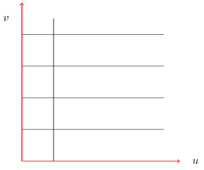
We can think of this one-dimensional reconstruction as a phase estimation along a single slice in the Fourier plane. A
generalization to two dimensions can be made by doing the same procedure for several slices as
described in Fig. 6. In fact, the requirement that a two-dimensional complex function be analytic,
is equivalent to satisfying the Cauchy-Riemann equations in both and (, 1990). The direction of the slices
is arbitrary, however for simplicity we reconstruct the phase along an
arbitrary set of perpendicular directions in the Fourier plane,
and noting that one can relate all slices through a single orthogonal slice, i.e. once the phase at the origin is set to zero,
the single orthogonal slice sets the initial values for the rest of the slices.
One can also require that the phase at a particular point
in the complex plane be exactly equal when reconstructed along or since each reconstruction is arbitrary up to a constant (piston) and a
linear term (tip/tilt). However, imposing this requirement results in a severely over-determined linear system. More precisely, by imposing equality
in points in the complex plane, and having slices (each with an unknown constant and linear term), results in a linear system of equations
and unknowns. Alternative methods of requiring slice consistency are a possible way of improving phase reconstruction, but are beyond
the scope of this paper.
The Cauchy-Riemman approach, with horizontal or vertical slices, and a single orthogonal slice, gives reasonably good results, however, it is not the only possible approach. We have also investigated Gerchberg-Saxton phase retrieval, Generalized Expectation Maximization, and other variants of the Cauchy-Riemann approach. It is premature to conclude which of these approaches is best at this time, given the limited imagery and SNR levels that have been explored. However, the Cauchy-Riemman approach has shown to give better results in a number of cases (, 2010).
6 Imaging capabilities
We investigated the imaging capabilities for simple objects555For preliminary study see Nuñez et al. (2010)., namely uniform disk-like stars, oblate rotating stars, binaries, and more complex images. For most of the objects that we consider, image reconstruction is not necessary, i.e. from the Fourier magnitude alone, one can extract radii, oblateness, relative brightness in binaries, etc. Estimation of these parameters is probably more accurate when extracted directly from Fourier magnitude data only, especially if some a-priori knowledge of the original image is available. However, measuring simple parameters from reconstructed images is the first step in quantifying reconstruction capabilities with IACT arrays. We assume no a-priori knowledge of the images that are being reconstructed, and then do a statistical study of the uncertainties of the reconstructed parameters.
6.1 Uniform disks
In order to quantify the uncertainty in the reconstructed radius, we
simulate data corresponding to magnitude stars () with disk radii up to
for 50 hours of exposure time666 This brightness and exposure time
correspond to uncertainties in the
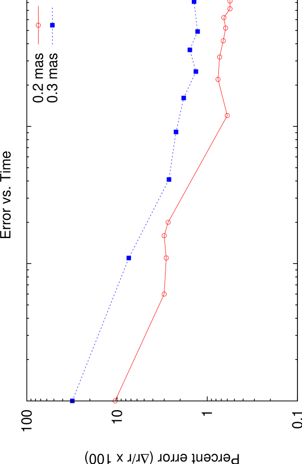
simulated data of a few percent. Such long exposure times can be reduced to
a few hours as is shown in Fig. 10. An example of such a reconstruction is shown in Fig.
7, where the radiance is shown in arbitrary units between 0 and
1. For a uniform disk, the reconstructed phase is null in the first lobe, and we find that the rms deviations from the true
phase are approximately in the null zone. A first look at the reconstruction in Fig. 7 reveals
that the edge of the reconstructed disk is not sharp, so a threshold in the
radiance was applied for measuring the radius. The radius is measured
by counting pixels above a threshold and noting that the area of the disk is
proportional to the number of pixels passing the threshold. After experimenting
with different radii, we chose the threshold for measuring the radius to be
0.2. We can now compare the simulated and
reconstructed radii as is shown in Fig. 8, where each point in the
Fig. corresponds to an individual simulation (including noise) and
reconstruction. Further optimization in the threshold for measuring the radius
should yield a slope even closer to unity in Fig. 8.
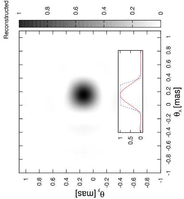
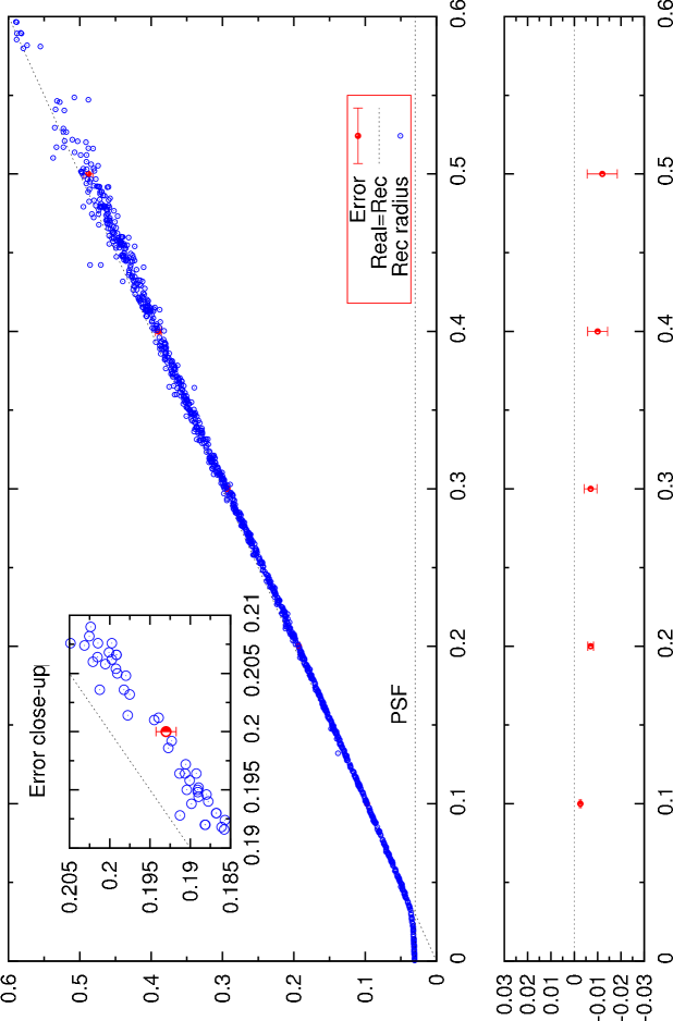
Fig. 8 clearly shows that stellar radii ranging from to can be measured with uncertainties ranging between sub-percent and a few percent (Figures 9 and 10). It can be seen from Fig. 8, that the uncertainty increases linearly as a function of the pristine (simulated) radius. This is due to a decrease in the number of baselines that measure a high degree of correlation when the angular diameter increases. As the pristine radius decreases, the distance to the first zero in the correlation increases as , so the number of telescopes contained within the airy disk increases as . Consequently, decreasing the pristine radius is equivalent to increasing the number of independent measurements by a factor of . Since the uncertainty decreases as the square root of the number of independent measurements, the error decreases linearly with the radius. For radii above , there are simply not enough baselines to constrain the Fourier plane information for image reconstruction. For radii greater than , the distance to the first zero in the degree of correlation is of the order of , but only baselines at and are capable of measuring the Fourier magnitude with more than 3 standard deviations (see eq. 2). In Fig. 10 we show the relative percent error (RMS of a statistic) as a function of time for two different radii, where it can be seen that a relative error of a few percent is achieved after only a few hours.

6.2 Oblate stars
For oblate stars we use the same magnitude and exposure
parameters that are used for disk-like stars. Uniform oblate stars can be
described by three parameters: the semi-major axis , the
semi-minor axis , and the inclination angle . Judging from the
limitations obtained from reconstructing disks, we produce
pristine images whose values for and are random numbers less than , and choose . The value
of the inclination angle also varies randomly between and
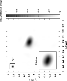
. A typical image reconstruction can be seen in Fig.
11.
After applying a threshold on pixel values as was done for disk shaped stars,
the reconstructed parameters are found by calculating the inertia
tensor of the reconstructed image. The eigenvalues and
eigenvectors of the inertia tensor provide information for the reconstructed values of , and
. To do this, we make use of the relation between the matrix eigenvalue and the semi-major/minor axes
, where is the integrated brightness. A similar relation for holds
for the semi-minor axis .
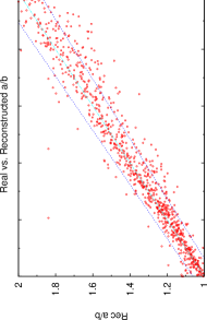
The resulting reconstructed semi-major/minor axes as a function of their real values have a similar
structure as the scatter plot for reconstructed radii shown in Fig.
8, and are well reconstructed up to within a few percent.
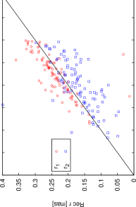
In Fig. 12, it can be seen how the uncertainty in the reconstructed oblateness
increases with increasing oblateness. As with disk shaped stars (section 6.1),
the uncertainty in the reconstructed semi-major/minor axes decreases as the square root
of the number of baselines measuring a high degree of correlation. Therefore, the
uncertainty in the reconstructed semi-major/minor axes is proportional to , and the error in the reconstructed oblateness
is proportional to .
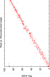
The reconstructed inclination angle as a function of the pristine angle is shown in Fig. 13, and several factors play a role in the uncertainty of the reconstructed value. For a fixed value of and , the orientation of the telescope array with respect to the main lobe of the Fourier magnitude determines the number of baselines that measure a high degree of correlation. The number of baselines that measure a high degree of correlation is greater when the main lobe of the Fourier magnitude is aligned with the or direction of the array (see Fig. 2), and is smaller by a factor of (assuming a uniform grid of telescopes) when its main axis is at with respect to the array. However, the uncertainty (proportional to spread of points) in Fig. 13 does not appear to be symmetric at and , and is smaller at . This due to the way the phase is reconstructed, i.e. due to the slicing of the Fourier plane along the or directions (see section 5). In the case of Fig. 13, the plane is sliced along the direction, with a single orthogonal reference slice along the direction. The main lobe of the Fourier magnitude of an oblate star has more slices passing through it when it is elongated along the direction (corresponding to an inclination angle of in image space), yielding a better reconstruction. This is in contrast to the orthogonal case of , where the main lobe of the Fourier magnitude has a smaller number of slices passing through it.
6.3 Binary stars
Simulated data are generated for magnitude binary stars (), and an exposure of
50 hours after noting that the uncertainty in the degree of correlation is of the order of a few percent (eq. 2).
Binaries stars are parameterized by the radii and of each star,
their separation , position angle , and relative brightness in arbitrary units between 0 and 1.
We generate pristine images with random parameters within
the following ranges: radii are less than , angular separations are
less than , the relative brightness per unit area is less than or equal to 1, and
the orientation angle is less than . A typical reconstruction can
be seen in Fig. 14.
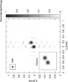
To measure the reconstructed parameters we identify the two brightest spots whose pixel values exceed
a threshold of 0.2. We then find the radius for each bright spot and its centroid position.
Identifying spots is a non trivial task
in noisy reconstructed images and our analysis sometimes fails to identify
the “correct” reconstructed spots. For example, a common issue is that
close reconstructed spots that are faintly connected by artifacts, are sometimes
interpreted as a single spot. It should be again stressed that image reconstruction may not be
the best way to measure reconstructed parameters. For example, the data can just as well be
fit by the general form of the Fourier magnitude of a resolved binary system (containing only a few parameters).
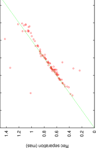
In Fig. 15, we show reconstructed angular separations
as a function of their real values. The reconstructed values of the angular separation are found
to within of their real values and cannot be much
larger than what is allowed by the smallest baselines. We find that stars separated
by more than are not well reconstructed since the variations in the Fourier magnitude
start to become comparable to the shortest baseline.
In Fig. 16 we show the reconstructed values of the radii as a function of their pristine
values. We find uncertainties in each of the reconstructed radii.
Aside from the angular separation, a variable that plays a role
in successfully reconstructing pristine radii is the
ratio of absolute brightness777Product
of relative brightness per unit area (in arbitrary linear units between 0 and 1) and relative area of both stars of both binary members. When
one of the two members is more than times brighter than the other, the fainter star
is found to be smaller than its pristine value, and sometimes not found at all when
one of the members is more than times brighter than the other. This is in part because the sinusoidal variations
in the Fourier magnitude start to become comparable to the uncertainty. For example: a non-resolved binary star
with one component 20 times brighter that the other, has relative variations of . With all the redundant baselines,
a few percent uncertainty in the measured degree of correlation is sufficient to accurately measure these variations.
However, when the binary components
are resolved, the relative variations decrease with increasing baseline and baseline redundancy is not sufficient to
reduce the uncertainty in the measurement of the Fourier magnitude. This signal to noise issue can of course be
improved by increasing exposure time.
There are also issues related to algorithm performance. One such problem has to do with the fit of the data to an analytic function (see section 4). When the scale of the fit (found by an initial Gauss fit) is found to be too small, too many basis elements are used to reconstruct the data, and high frequency artifacts appear in reconstructions. Small initial scales are typically related to the binary separation as opposed to the size of individual components, and it is the latter which correctly sets the scale of the fit. Artifacts may be then mistaken for binary components, and incorrect reconstructed parameters may be found. Results improve significantly when either the correct scale is set or (model-independent) image post-processing is performed (see section 6.5).
6.4 Featured images
We now present two examples of more complex images, and show that the capabilities can, to a large extent, be understood from results of
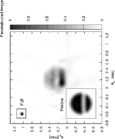
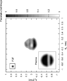
less complex images, such as uniform disks and binaries. In Fig. 17 we show the reconstruction of a star with a dark
band (obscuring disk), corresponding to a magnitude star and 10 hrs of observation time. The metric used to quantify the
agreement with the pristine image (bottom left corner of Fig. 17) is a normalized correlation888For two images and , the normalized correlation is , where and are the standard deviations of images and .
whose absolute value ranges between 0 (no correlation) and 1 (perfect correlation/anti-correlation). To quantify the uncertainty in the correlation, we perform the noisy simulation and reconstruction several times, and find the standard deviation of the degree of correlation. In the case of Fig. 17, the correlation is . Note that the uncertainty in the correlation is apparently small, and the image reconstruction is not perfect, which implies that the reconstruction is not only affected by the SNR level, but also by the reconstruction algorithm performance.
In order to determine the confidence with which we can detect the feature (dark region within the disk), this correlation is compared to the correlation of the reconstruction, and a featureless image, i.e. a uniform disk whose radius matches the radius of the pristine image. This comparison allows us to quantify the confidence with which we actually detect the feature (dark spot). Consequently, the correlation of the reconstructed image with a uniform disk is , which is lower by 61 standard deviations.
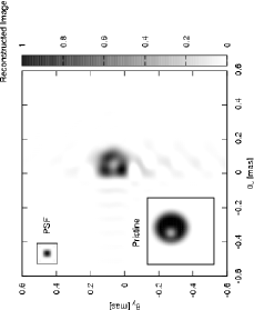
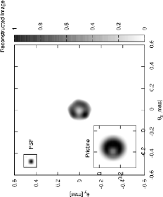
Another example of a complex image reconstruction can be seen in Fig. 18. Here we show the reconstruction of a star with a dark spot, whose correlation with the pristine image is . We can compare this correlation with the correlation of the reconstructed image and a uniform disk, which is (lower by 30 standard deviations).
For both examples, we also calculate the correlation with the pristine image as a
function of the angular scale (in ) of the pristine image. We then find the
degree of correlation of each reconstruction and its pristine image, and also the
degree of correlation of the reconstruction with a uniform disk. By comparing
these two correlation values, we can find the
smallest feature that can be reconstructed. Below some point we
no longer distinguish between the reconstruction of the featured image and that
of a uniform disk. We find that the smallest feature that
can be reconstructed is close to . This can already be seen
from the order of magnitude estimate made in section 2 and a comparable
value of is found in section 6.1. When pristine images
have angular sizes greater than , the degree of
correlation drops significantly due to lack of short baselines. Note that
this value is higher than what is found in section 6.1. This is due to
higher signal to noise ratio in the simulated data corresponding
to Figures 17 and 18. The resolution limits
discussed in turn correspond to effective resolution elements (pixels).
6.5 Post-processing
Image post-processing is performed in order to improve the raw images presented above. The type of post-processing that is currently being investigated is analogous to the data analysis performed in conventional amplitude interferometry. In this analysis, the image is slightly modified so as to maximize the agreement between the data and the magnitude of the Fourier transform of the reconstructed image. See (2009) for details. Also, one can introduce additional and very general constraints to this maximization procedure, but this is beyond the scope of this paper. Such an analysis depends strongly on the starting image, which can be provided by the analysis presented in this paper. An example of image post-processing performed on the oblate star of Fig. 19 is shown in Fig. 20.
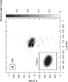
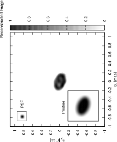
We have performed this type of post-processing on the images in Figures 17 and 18 using the MiRA software (, 2009), and we obtain the ones shown in Figures 21 and 22. Aside from optimizing agreement with the data, no additional constraints are imposed. These preliminary results show the overall reduction in noise and improvement in the sharpness of the reconstructed images. A systematic study of the improvements with image post-processing is currently being investigated (, 2011).
7 Conclusions
We perform a simulation study of the imaging capabilities at of an IACT array consisting of 97 telescopes separated
up to a . This is a preliminary design for the CTA project, expected to be operational in 2018. Our method uses a model-independent
algorithm to recover the phase from intensity interferometric data. We test the method on images of increasing degrees
of complexity, parameterizing the pristine image, and comparing the reconstructed parameter with the
pristine parameter. We now summarize our results and briefly discuss how fundamental stellar parameters can be constrained with the methods described above.
We first find that for bright disk-like stars (), radii are well reconstructed from to .
Even though using a Cauchy-Riemann based approach to recover images
might not be the most efficient way to measure stellar radii, such a study
starts to quantify the abilities of measuring other scale parameters in
more complicated images (oblateness, distance between binary components,
etc.). The range of angular radii that can be
measured with a CTA-like array () will complement existing measurements () (, 2001). With the aid of
photometry, the effective temperature999Defined as , where is the radius, is the luminosity, and is the Stephan-Boltzmann constant. scale of stars within can be extended. Multi-wavelength angular diameter measurements will also reveal the wavelength dependence of limb-darkening (, 2010), and such measurements can be used to constrain energy transport models as is done in amplitude interferometry (, 2005).
For oblate stars, similar results for extracting geometrical parameters are found. Due to the relative ease of SII to observe at short () wavelengths, measuring fundamental parameters of hot B type stars is possible. B stars are particularly interesting since rapid rotation, oblateness, and mass loss are a common feature. We show that oblateness can be accurately measured, and a next step will be to quantify the capabilities of imaging realistic surface brightness distributions in hot stars. By imaging brightness (temperature) distributions, we will be able to study effects such as limb darkening and mass loss in hot massive stars (, 2009), as well as gravity darkening (, 1924).
Binary stars are well reconstructed when one of the members is not much brighter (three times as bright) than the other,
and when they are not too far apart (). As with amplitude interferometry, SII, along with spectroscopy, will allow the determination masses and orbital parameters in binary stars. If measured with enough precision () (, 1991), the determination of the mass can be used to test main sequence stellar models. An advantage of using an array such as the one used in this study, is that individual radii can be resolved. An interesting phenomena to be studied with interacting binary stars is mass transfer (e.g. Zhao et al. 2008), and capabilities for imaging this phenomena can be further investigated.
Two examples of reconstructions of more complex images are presented, and demonstrate the capability to resolve features in the sub-milliarcsecond scale. Results show improvement when post-processing is performed. An optimization procedure improves the image reconstructions found by the methods presented above by maximizing their agreement with the data. A more comprehensive study of reconstructions of complex images is currently being performed.
Appendix A. Cauchy-Riemann phase recovery
Recall that since SII can only allow to measure , the phase information is lost, and we would like to recover it for imaging purposes, with only the magnitude information. If we denote , where , we obtain the following relations from the Cauchy-Riemann equations101010The C-R equations can be applied because “I” is a polynomial in z.:
| (4) | |||||
| (5) |
where we have defined as the log-magnitude. Notice the relation between the magnitude and the phase. By using the Cauchy-Riemann equations we can write the log-magnitude differences along the real and imaginary axes as:
| (6) | |||||
| (7) |
If the log-magnitude were available along purely the or the axes, we could solve the previous two equations for the phase.
However, notice that because ,
we can only measure the log-magnitude on the unit circle in the complex space ().
In general, we can write the log-magnitude differences along the unit circle as
| (9) | |||||
Here corresponds to phase differences along a direction perpendicular to , that is, perpendicular to the unit circle in the plane. We are however interested in obtaining , so that we can integrate along the unit circle.
The general form of can be found by taking second derivatives in eq. (5) and thus noting that is a solution of the Laplace equation in the complex plane.
| (11) |
The general solution of in polar coordinates () is (, 1998)
| (12) |
where terms singular at the origin () have been omitted. These singular terms lead to ambiguous reconstructions including flipped images and have not been found to be essential for most reconstructions.
Now taking the difference of along the radial direction we obtain
| (13) |
Note from eq. (Appendix A. Cauchy-Riemann phase recovery) that the length in the complex plane associated with is , and that the length associated with is . Now setting , , and for simplicity of presentation, expanding for small , we obtain
| (14) |
So now the coefficients and can be found using equations (9-Appendix A. Cauchy-Riemann phase recovery) from the measured , and thus can be found in the complex plane, with an uncertainty in and . The coefficients and can be calculated by performing the following integrals:
| (15) |
| (16) |
Note however that the previous expressions must exist, which is not the general case. More explicitly, if the magnitude is zero, the log-magnitude is singular. When imaging finite objects in image space, there will always be zeros in the magnitude of the Fourier transform. In practice we are always sample limited and nothing prevents us from calculating and approximately.
References
- (1) Andersen J., 1991, AAPR, 3, 91
- (2) Aufdenberg J. P., Ludwig H. G., Kervella P., 2005, ApJ, 633, 424
- Aufdenberg et al. (2006) Aufdenberg J. P. et al., 2006, ApJ, 645, 664
- (4) Aufdenberg J. P., Ridgway S., White R., 2009, astro2010: The Astronomy and Astrophysics Decadal Survey, 2010, 8
- Baldwin et al. (1996) Baldwin J. E. et al., 1996, A&A, 306, L13
- Bernlöhr (2008) Bernlöhr K., 2008, American Institute of Physics Conference Series, 1085, 874
- Bessell (1979) Bessell M. S., 1979, PASP, 91, 589
- CTA Consortium (2010) CTA Consortium, 2010, arXiv:1008.3703
- (9) Dravins D. et al., 1994, Proc. SPIE 2198, 289
- Fienup (1981) Fienup J. R., 1981, JOSA, 71, 1641
- (11) Friend D. B., Abbott D. C., 1986, ApJ, 311, 701
- (12) Hanbury Brown R., 1974, The Intensity Interferometer, Taylor & Francis, London.
- (13) Haniff C. A., 2001, Galaxies and their Constituents at the Highest Angular Resolutions, 205, 288
- (14) Holder J., LeBohec S., 2006, ApJ 649, 399
- (15) Holmes R. B., Belen’kii M. S., 2004, JOSA 21, 697
- (16) Holmes R. B., Nuñez P. D., LeBohec S., 2010, Proc. SPIE 7818
- (17) Hörmander L., 1990, An introduction to complex analysis in several variables. Elsevier Science
- (18) Jackson J. D., 1998, Classical Electrodynamics, 3rd Edition, by John David Jackson, Wiley-VCH.
- (19) Kervella P., 2008, IAU Symposium, 252, 405
- (20) Labeyrie A., Lipson S. G., Nisenson P., 2006, An Introduction to Optical Stellar Interferometry, by A. Labeyrie, S. G. Lipson and P. Nisenson, Cambridge University Press, Cambridge
- Lafrasse et al. (2010) Lafrasse S., Mella G., Bonneau D., Duvert G., Delfosse X., Chelli A., 2010, VizieR Online Data Catalog, 2300, 0
- Lawrence et al. (1990) Lawrence T. W., Fitch J. P., Goodman D. M., Massie N. A., Sherwood R. J., 1990, Proc. SPIE, 1237, 522
- (23) LeBohec S. et al., 2010, Proc. SPIE, 7734, 7734
- (24) Maeder A., 1997, A&A, 321, 134
- (25) Maier G., preprint(arXiv:0907.5118)
- (26) Martin E. L., Claret A., 1996, A&A, 306, 408
- (27) Monnier J. D., 2007, Bulletin of the American Astronomical Society, 38, 854
- Monnier et al. (2007) Monnier J. D. et al., 2007, Science, 317, 342
- (29) Mozurkewich D. et al., 2003, ApJ 126, 2502-2520
- Nuñez et al. (2010) Nuñez P. D., Lebohec S., Kieda D., Holmes R., Jensen H., Dravins, D., 2010, Proc. SPIE 7734
- (31) Nuñez P. D. et al., 2011, In prep.
- (32) Ridgway S. et al., 2009, astro2010: The Astronomy and Astrophysics Decadal Survey, 2010, 247
- (33) Saio H. et al., 2006, ApJ, 650, 1111
- (34) Thiebaut E., 2009, New Astron. Rev. 53, 312
- (35) Verhoelst T., van Aarle E., Acke B., 2007, A&A, 470, L21
- (36) von Zeipel H., 1924, MNRAS, 84, 665
- Zhao et al. (2008) Zhao M. et al., 2008, ApJ, 684, L95