Adaptive multiple subtraction with wavelet-based complex unary Wiener filters

Abstract

Adaptive subtraction is a key element in predictive multiple-suppression methods. It minimizes misalignments and amplitude differences between modeled and actual multiples, and thus reduces multiple contamination in the dataset after subtraction. Due to the high cross-correlation between their waveform, the main challenge resides in attenuating multiples without distorting primaries. As they overlap on a wide frequency range, we split this wide-band problem into a set of more tractable narrow-band filter designs, using a 1D complex wavelet frame. This decomposition enables a single-pass adaptive subtraction via complex, single-sample (unary) Wiener filters, consistently estimated on overlapping windows in a complex wavelet transformed domain. Each unary filter compensates amplitude differences within its frequency support, and can correct small and large misalignment errors through phase and integer delay corrections. This approach greatly simplifies the matching filter estimation and, despite its simplicity, narrows the gap between 1D and standard adaptive 2D methods on field data.

1 Introduction

Multiples correspond to unwanted coherent events related to wave field reflection bounces on given surfaces. We refer to the comprehensive survey in Verschuur, (2006) for a detailed description. Their attenuation (Verschuur and Berkhout,, 1992) represents one of the greatest challenges in past and present seismic processing, since the January 1948 issue of Geophysics. Their processing mainly relies on two types of approaches: (1) primary/multiple discrimination based on different velocities and reflections and (2) periodicity and predictability.

The first approach maps data to a transformed domain with minimum overlap between primaries and multiples. Transformed domain filters subsequently attenuate multiples or select primaries of interest. The filtered data is finally mapped back to data domain, using an appropriate inverse transform. Common tools include stacking combined with Normal Move Out (NMO), homomorphic filtering (Buttkus,, 1975), $f-k$ (Wu and Wang,, 2011), and $\tau-p$ representations (Nuzzo and Quarta,, 2004), or alternative breeds — parabolic, hyperbolic — of the Radon transform (Hampson,, 1986; Trad et al.,, 2003; Nowak and Imhof,, 2006), with pros & cons discussion in Kabir and Verschuur, (2007).

The second approach includes prediction filters and variations thereof (Taner,, 1980; Abma et al.,, 2005; Spitz et al.,, 2009), also termed identification, updating, shaping, sequential or matching filters in electrical engineering literature (Ristow and Kosbahn,, 1979) or predictive deconvolution (Taner et al.,, 1995). Recently, modeling based techniques, such as surface-related multiple estimation (SRME), have demonstrated excellent performance, allowing data-driven multiple removal (Verschuur and Berkhout,, 1992; Weglein et al.,, 1997; Lin et al.,, 2004) or model-driven, wave-equation based, multiple removal (Pica et al.,, 2005; Weisser et al.,, 2006). These methods, based on multiple models, consist in predicting then subtracting multiple events from original seismic data.

To compensate for mismatches, an adaptive subtraction is usually performed (Verschuur and Berkhout,, 1997; Dragoset et al.,, 2010); however, more direct subtraction, for instance when formulated as an inverse problem, is possible (see, e.g., Amundsen et al.,, 2001; van Groenestijn and Verschuur,, 2009). The adapted model is commonly obtained through a linear Wiener-type filter (Robinson and Treitel,, 1967) that minimizes the energy of the difference between data and model. Although primaries and multiples, generated from the same source, are not fully uncorrelated, or orthogonal, least square error (LSE) solutions are widespread, mainly due to their computational simplicity. To reduce the distortion of primaries due to their cross-correlation with multiples, these matching filters are usually applied in two steps in practical cases. Long filters compensate global amplitude, waveform and time-shift differences, then shorter filters correct time variant discrepancies.

The observation on primaries and multiples cross-correlation leads to more hybrid methods, mixing both transform and prediction approaches. Improvements may reside in different strategies. Either the use of more robust objective matching criteria than LSE based ones, such as those based on the $L_{1}$ norm (Guitton and Verschuur,, 2004), or independence-based subtraction (Kaplan and Innanen,, 2008) are efficient alternatives. Simultaneous estimation of sets of filters based on a broader quantity of information is another option, e.g., in multichannel adaptation (Wang,, 2003). A suitable data representation may further serve adaptive subtraction (Taner, (1980) with radial suppression, Berkhout and Verschuur, (2006) with focal transform). A recent trend focuses on multiscale or wavelet-like approaches (Jacques et al.,, 2011), which may better promote sparsity in exploiting slight differences in primaries and multiple spectra. Pokrovskaia and Wombell, (2004); Ahmed, (2007) use standard discrete wavelet transforms. Herrmann and Verschuur, (2005); Donno et al., (2010); Neelamani et al., (2010) follow a twist towards curvelets, sometimes regarded as a local multiscale Radon transform (de Hoop et al.,, 2009).

In many cases, the choice of the type and length of the matching filter, whatever the domain, needs careful parameter selection and testing, and requires computational resources. With our method, we aim at overcoming this issue by decomposing a complicated wide-band problem into a set of more tractable narrow-band problems, through a wavelet transform. In the proposed approach, model-based multiple removal is solely based on 1D traces, and hence does not compete directly with higher dimensional (Dragoset et al.,, 2010), regularized (Guitton,, 2004; Fomel,, 2009) or robust approaches (Herrmann and Verschuur,, 2005). More precisely, comparing with existing literature, we retain the following three concepts: 1) non-stationary Wiener matching filters (Lines,, 1996; Fomel,, 2009), 2) complex trace processing (Monk,, 1993; Wang,, 2003; Huo and Wang,, 2009), 3) continuous wavelet frames (Sinha et al.,, 2005).

The adopted complex Morlet wavelet frame emulates limited-scale complex derivatives (Monk,, 1993). The adaptation in the wavelet domain is performed at each scale with a complex "unary" filter, e.g., a one-coefficient matching operator (Pesquet and Leporini,, 1997), accounting for localized phase and amplitude variations between data and model. The flexible redundancy and the "complex trace" effect of this wavelet frame allow a better management of time variability in model misalignment errors, at the price of a less intuitive interpretation of the designed subtraction operator, due to the complex interplay between unary filters and wavelet decomposition. The complex curvelet method, proposed by Neelamani et al., (2010), can be viewed as performing unary Wiener filtering in a complex-valued curvelet domain. With the proposed algorithm, we aim at a better understanding of the intricate relationship between a sparsifying transform and its associated matched filtering. Its flexibility both resides in choices for a quasi-analytic wavelet and its scale discretization, to better adapt variations in data character and sampling. The algorithm alleviates some constraints of the curvelets (either real or complex) such as a relatively high memory footprint and its fixed dyadic frequency decomposition. However, as strictly 1D, it does not capitalize the information given by neighboring traces. Despite this, the closed-form of the matching filter may be beneficial in keeping low complexity, computational speed and possible parallelization. Being nevertheless rather competitive to 2D techniques, it may fit sparsely or non-uniformly sampled datasets.

2 Methodology

A classical 1D trace observation model is:

$$d[n]=p[n]+m[n]+w[n]\,,$$ (1)

where $d[n]$, $p[n]$, $m[n]$ and $w[n]$ denote the recorded data, primary events, multiples and background noise, respectively, at discrete time index $n$.

2.1 Complex wavelet transform decomposition

We perform a time-scale decomposition of each data $d[n]$ and multiple model $x[n]$ traces with discrete wavelet frame approximations to continuous wavelet transform (CWT). We refer to Jorgensen and Song, (2009) and references therein for comparison between discrete and continuous wavelet transforms. We choose the complex Morlet wavelet since it yields a simple interpretation of amplitude and phase delay in the transformed domain.

The mother Morlet wavelet is approximately analytic and writes:

$$\psi(t)=\pi^{-1/4}e^{-i\omega_{0}t}e^{-t^{2}/2}\,,$$ (2)

where $\omega_{0}$ is the central frequency of the modulated Gaussian, $t$ denoting the continuous time variable. A standard choice of $\pi\sqrt{2/\ln(2)}$ for the central frequency halves side-lobe amplitude with respect to the main lobes.

The associated discrete family of functions is defined as a sampling of the mother wavelet:

$$\psi_{r,j}^{v}[n]=\frac{1}{\sqrt{2^{j+v/V}}}\psi\!\left(\frac{nT-r2^{j}b_{0}}{2^{j+v/V}}\right)\,,$$ (3)

with $T$ the sampling rate and $V$ the number of voices per octave. Indices $r,j\in\mathbb{Z}$ and $v\in[0,\ldots,V-1]$ denote, respectively, discretized time, octave, and voice. Finally, $b_{0}$ stands for the sampling period at scale zero, $j=v=0$. Its redundancy, of approximately $2V/b_{0}$, may be adapted to the expected computational efficiency.

The time-scale representation of trace $d[n]$, for instance, is given by the inner product:

$$\mathbf{d}=d_{r,j}^{v}=\left\langle d[n],\psi_{r,j}^{v}[n]\right\rangle=\sum_{n}d[n]\overline{\psi_{r,j}^{v}[n]}\,,$$ (4)

and written in bold, with indices dropped for more generality, accounting for the whole trace, or a windowed portion of it. Windowing in time-scale domain improves the localization in complex unary filters estimation. Expression $\overline{\psi_{r,j}^{v}[n]}$ denotes the complex conjugate of $\psi_{r,j}^{v}[n]$.

Suppose $\hat{\mathbf{d}}$ results from some time-scale correction or processing of $\mathbf{d}$, here model matching and subtraction. Then the resulting filtered trace is synthesized back to the time domain as a sum of the dual frame components, $\widetilde{\psi}_{r,j}^{v}[n]$,

$$\hat{d}[n]=\sum_{r}\sum_{j,v}\hat{d}_{r,j}^{v}\widetilde{\psi}_{r,j}^{v}[n]\,,$$ (5)

weighted by the corrected signal $\hat{d}_{r,j}^{v}$, for instance here with multiples subtracted. Illustrations of corresponding time-scale raw and processed data are provided in Ventosa et al., (2011). With sufficient redundancy, $\widetilde{\psi}[n]$ can be approximated by $\psi[n]$ up to a constant multiplicative factor (see, e.g., Vetterli and Kovačević,, 1995).

The discriminative power of the wavelet frame helps reformulate the design of a long matching filter into combined global and local optimum complex unary filters, minimizing the error between multiple events and their matched model. The straightforward group-delay estimation allowed by Morlet wavelets, together with frame redundancy, helps avoiding reconstruction artifacts observed with non-redundant discrete wavelet processing (Gilloire and Vetterli,, 1992).

2.2 Unary filter estimation: amplitude and delay

When the group delay difference between model and multiple sequences is less than half a period at all scales, it can be corrected in the time-scale domain following an LSE approach. The optimum unary filter at a given wavelet scale, either in local or global windowed portions of the trace, is defined as the complex scalar $a$ which, multiplied by the time-scale decomposed multiple model $\mathbf{x}$, minimizes the mean square error $\xi(a)$ with the decomposed input dataset $\mathbf{d}$:

$$a_{\textrm{opt}}=\mathop{\arg\min}_{a}\xi(a)=\mathop{\arg\min}_{a}\left\|\mathbf{d}-a\mathbf{x}\right\|^{2}$$ (6)

where the phase of $a_{\textrm{opt}}$ compensates small delays.

This method is efficient, provided the above small group delay condition is satisfied (Neelamani et al.,, 2010). Otherwise, i.e., when the cross-correlation peak departs from the zero delay sample, faulty $a_{\textrm{opt}}$ estimation in equation 6 requires a redesign of the filter.

Two options can be conceived to add robustness against high fractional delays, while keeping with the unary filter approach: either to design filters with a high group delay, or to add a gross group delay correction first and then to apply the previous unary filter for fine group delay correction. In contrast with the Fourier transform, wavelets’ fast decay strongly limits the maximum group delay correction on the first option. Hence, we focus exclusively on the second one. However, high group delay filters enable a relatively simple scale-wise unary filter design, that could reinforce matching in noisy scenarios, in applications where the specifications of group-delay range are smaller than the effective time support of the chosen wavelets.

We thus introduce a delay term into the above unary filter to yield higher delay robustness, while keeping an LSE criterion. This amounts to finding optimum $a$ and delay $l$ that minimize:

$$\xi(a,l)=\sum_{r}\left|d_{j}^{v}[r]-a_{j}^{v}x_{j}^{v}[r-l]\right|^{2}=\left\|\mathbf{d}-a\mathbf{x}_{l}\right\|^{2}\,,$$ (7)

where $\mathbf{x}_{l}$ denotes a delay of $\mathbf{x}$ by $l$ samples, sequences $d_{j}^{v}[r]$ and $x_{j}^{v}[r]$ are complex and the $\sum$ symbol denotes a locally weighted sum along odd $L$ consecutive samples around index $r$. We opt to drop all subscripts for $a_{\textrm{opt}}$ for clarity. It is understood that this algorithm may be applied either locally or globally, depending on problem constraints.

For a given delay $l$, optimum $a_{\textrm{opt}}$ yields orthogonality between filtered signal $\mathbf{y}=\mathbf{d}-a_{\textrm{opt}}\mathbf{x}_{l}$ and adapted model $a\mathbf{x}_{l}$, which writes in inner product form as:

$$\left\langle\mathbf{d}-a_{\textrm{opt}}\mathbf{x}_{l},a\mathbf{x}_{l}\right\rangle=0\quad\forall a\neq 0\,.$$ (8)

By developing and applying linearity on the first argument and conjugate linearity on the second one, we obtain:

$$\overline{a}\left(\left\langle\mathbf{d},\mathbf{x}_{l}\right\rangle-a_{\textrm{opt}}\left\langle\mathbf{x}_{l},\mathbf{x}_{l}\right\rangle\right)=0\quad\forall a\neq 0$$ (9)

and therefore

$$a_{\textrm{opt}}[l]=\frac{\left\langle\mathbf{d},\mathbf{x}_{l}\right\rangle}{\left\|\mathbf{x}_{l}\right\|^{2}}=\frac{\sum_{r}d_{j}^{v}[r]\overline{x_{j}^{v}[r-l]}}{\sum_{r}\left|x_{j}^{v}[r-l]\right|^{2}}\,,$$ (10)

i.e., the unary Wiener filter solution for complex signals.

Note that instead of performing a direct measurement of the fractional delay, or equivalently of the group delay, we estimate the phase delay at each scale or frequency component. When the signal-to-noise ratio (S/N) is high, all meaningful phase components are sufficiently well estimated. However, when the S/N decreases, moderate phase errors made at key scale components may induce huge errors on group delay. As a consequence, we have to ensure that the phase of $a_{\textrm{opt}}$ varies smoothly in scale for important components.

Several criteria, well adapted to the nature of the seismic signals, can be chosen in the selection of the optimum delay. The optimum integer delay, in LSE sense, is selected among all sub-optimal $a_{\textrm{opt}}[l]$ as the one minimizing $\xi(a,l)$:

$$l_{\textrm{opt}}=\mathop{\arg\min}_{l}\xi(a_{\textrm{opt}}[l])\,.$$ (11)

Alternatively, due to the importance of waveform over amplitude, we can define the optimum delay as the one that maximizes the normalized cross-correlation between the adapted model and the data, commonly called coherence (Neidell and Taner,, 1971; Taner et al.,, 1979; Schimmel and Paulssen,, 1997),

$$l_{\textrm{opt}}=\mathop{\arg\max}_{l}\>C[l]$$ (12)

being

$$C[l]=\textrm{Re}\left[\frac{\left\langle\mathbf{d},a_{\textrm{opt}}[l]\mathbf{x}_{l}\right\rangle}{\left\|\mathbf{d}\right\|\left\|a_{\textrm{opt}}[l]\mathbf{x}_{l}\right\|}\right]\,,$$ (13)

where we focus on the real part of the normalized cross-correlation.

The use of unary filters enables two important simplifications of the previous equations. Applying conjugate linearity in the second argument of the inner product and positive scalability of the norm gives:

$$l_{\textrm{opt}}=\mathop{\arg\max}_{l}\>\textrm{Re}\left[\frac{\overline{a_{\textrm{opt}}[l]}}{\left|a_{\textrm{opt}}[l]\right|}\frac{\left\langle\mathbf{d},\mathbf{x}_{l}\right\rangle}{\left\|\mathbf{d}\right\|\left\|\mathbf{x}_{l}\right\|}\right]\,.$$ (14)

Namely, the normalized cross-correlation between the adapted model and the data only depends on the phase of the optimum unary filter and the normalized cross-correlation between the original model and the data.

Slighty better results can be obtained with an independent fine selection of the window functions used in the estimation of the unary filter and the normalized cross-correlation, equations 10 and 13. However, even more important to us, when these weighted sums are chosen equal, the normalized cross-correlation of the corrected sequence is equivalent to the cosine of the angle between $\mathbf{d}$ and $\mathbf{x}_{l}$. This can be shown noticing that $\overline{a_{\textrm{opt}}[l]}/\left|a_{\textrm{opt}}[l]\right|$ can be written depending on $\mathbf{d}$ and $\mathbf{x}_{l}$ from its definition in equation 10,

$$\frac{\overline{a_{\textrm{opt}}[l]}}{\left|a_{\textrm{opt}}[l]\right|}=\frac{\overline{\left\langle\mathbf{d},\mathbf{x}_{l}\right\rangle}}{\left|\left\langle\mathbf{d},\mathbf{x}_{l}\right\rangle\right|}\>.$$ (15)

As a consequence, the normalized cross-correlation is totally independent of the optimum unary filter in this particular case,

$$l_{\textrm{opt}}=\mathop{\arg\max}_{l}\frac{\left|\left\langle\mathbf{d},\mathbf{x}_{l}\right\rangle\right|}{\left\|\mathbf{d}\right\|\left\|\mathbf{x}_{l}\right\|}$$ (16)

and the coherence value measured is always real and positive. When no window is used, this criterion reduces to maximum cross-correlation between data and predicted multiples.

This configuration enables an important reduction on the computational cost when the normalized cross-correlation estimator is used, as it enables a direct estimation of the optimum integer delay, without having to estimate the optimum unary filter for each candidate. Concisely, we first gauge an integer delay, equation 16, to rectify large time shifts; we then estimate the optimum unary filter, equation 10, to shrink amplitude and remaining delay differences.

3 Examples

Figure 1: Subtraction results on a synthetic dataset with two events (a) with multiple model (b), using: (c) standard 1D adaptation, (d) 1D complex unary filters in time-scale, and (e) standard 2D adaptation.

Figure 2: Portion of common shot gather 1551. (a) Recorded data. (b) Multiple model.

Figure 3: Portion of first channel gather. (a) Recorded data. (b) Multiple model.

Figure 4: Subtraction results on common shot gather 1551. Filtered data (a) with the standard 1D adaptive filter, (b) with 1D complex unary filters in the time-scale domain, and (c) with standard 2D adaptive filter in the time-space domain. (d) Difference between (b) and (c). P and M mark discrepancies on primary and multiple events, respectively.

Figure 5: Subtraction results on the first channel gather. (a) Standard 1D adaptive filter. (b) 1D complex unary filters in the time-scale domain. (c) Standard 2D adaptive filter in the time-space domain. See Figure 6 for a zoom on the delimited zone.

Figure 6: Zoom on traces between shot number 1400 and 1700 of Figure 5. (a) Recorded data. (b) Original model. Filtered data with (c) standard 1D adaptive filters, (d) 1D complex unary filters in the time-scale domain, and (e) standard 2D adaptive filters. P marks discrepancies on primary events.

Figure 7: Superimposition of selected waveforms. (a) Recorded data and original model with a small positive delay. (b) Recorded data and adapted model with 1D complex unary filters in time-scale. (c) Recorded and filtered data.

Figure 8: Near offset stack of the raw data. P and M mark primary and multiple events, respectively.

Figure 9: Near offset stacks of filtered data using (a) standard 1D adaptive filters, (b) 1D complex unary filters in time-scale, and (c) standard 2D adaptive filters.

Figure 10: Near offset stacks of the difference between the raw data and the filtered data using (a) standard 1D adaptive filters, (b) 1D complex unary filters in time-scale, and (c) standard 2D adaptive filters. P marks overadaptation to primary events.

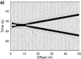
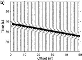
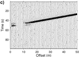
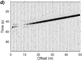
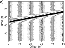
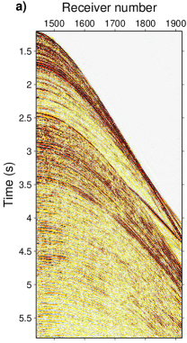
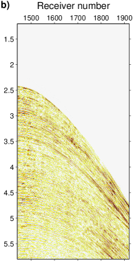
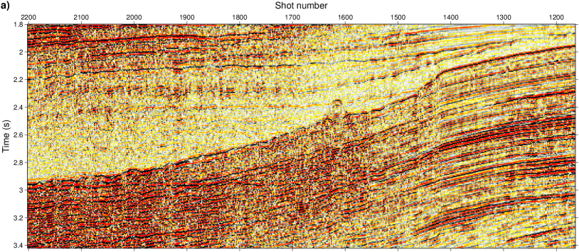
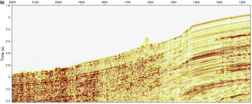
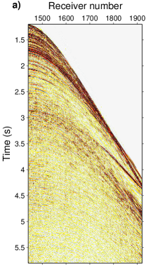
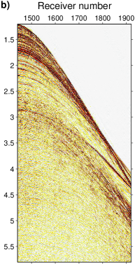
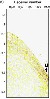
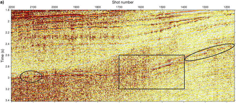
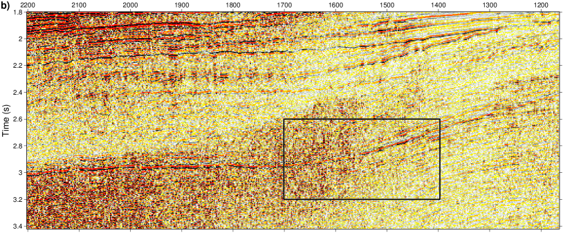
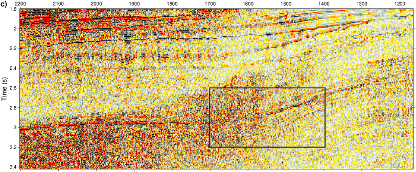
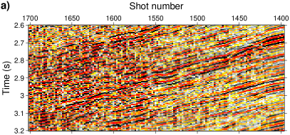
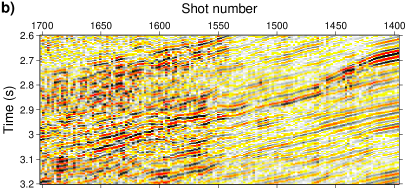
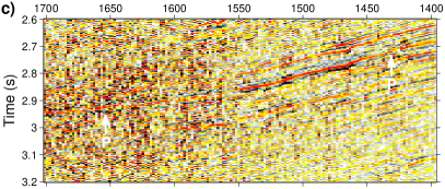
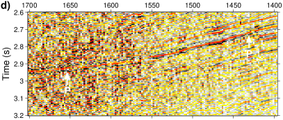
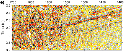
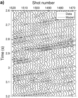
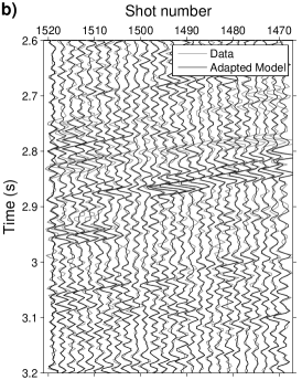
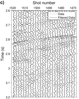
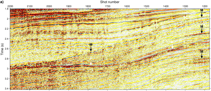
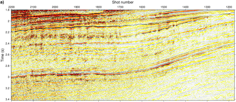
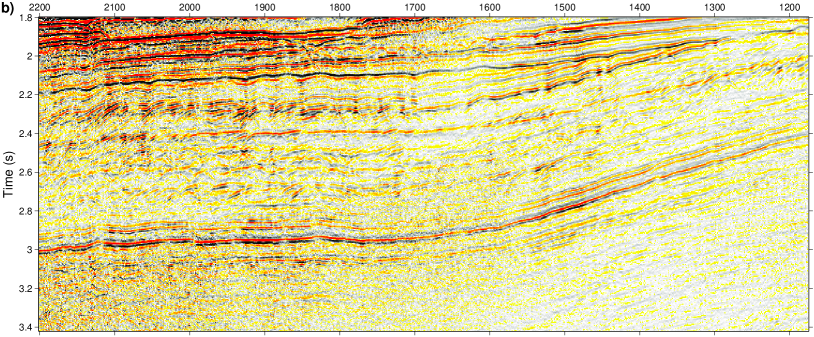
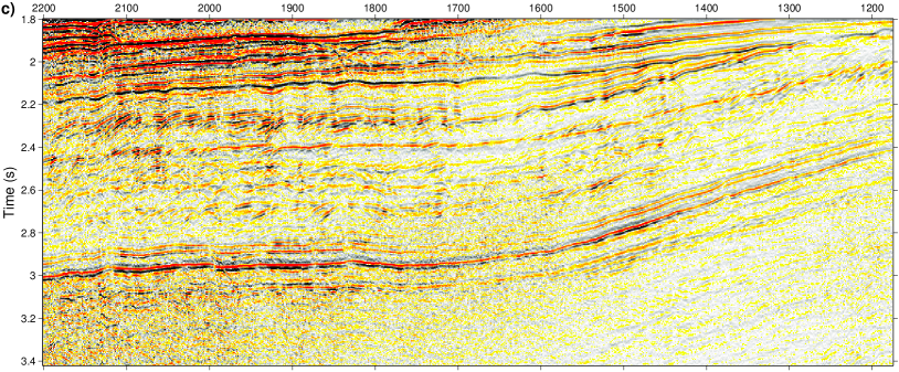
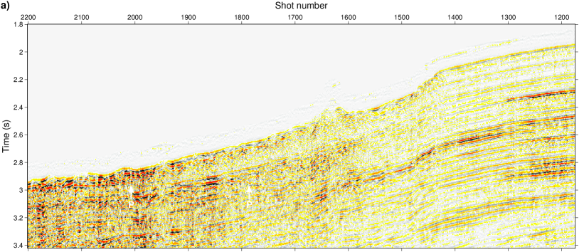
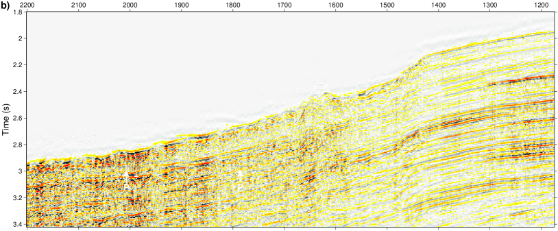
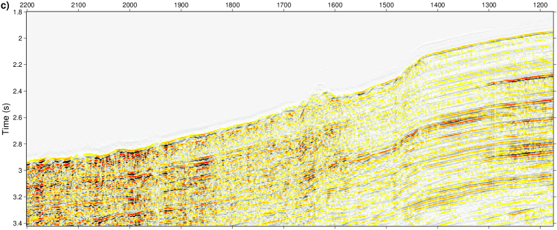
Figure 1a represents synthetic data with two intersecting dipping events with wavelets of equal amplitude and frequency content; Figure 1b shows the multiple model. As expected, 1D algorithms (1D filters computed in 1D data windows) behave similarly and fail to properly cope with the intersection. However, a dataset showing single primary and multiple events with identical wavelet shape is not completely realistic. In practice, variations in wavelet shapes associated with uncorrelated time arrivals of primaries and multiple greatly contribute to the success of adaptation in a given time frame. Thus, better behavior of the proposed algorithm on actual data is expected. Firstly, it enhances primaries and multiples discrepancies in the wavelet domain. Secondly, it enables cross-correlation reduction using larger window frames containing several signals, as demonstrated in the following field example.

The examples shown in Figures 2a and 3a are taken from a 3D real marine dataset, in common shot and channel gather, respectively. The main objective is to uncover primaries masked by strong multiple events using a multiple model. The 3D-SRME model (Pica et al.,, 2005) shown in Figures 2b and 3b achieves good precision on the near and mid offset range. We compare the proposed method based on 1D complex unary filters in wavelet domain, with reference algorithms based on standard 1D and 2D adaptive filters. Figures 4 and 5 represent subtraction results in common shot and channel gathers, respectively. Additional details are provided in Figures 6 (for improved visual amplitude assessment) and 7 (for accurate waveform comparison), to better illustrate the main features in data and differences between algorithms.

With a standard two-step method, the global step mainly contains waveform and time-shift corrections, combined with a global amplitude adaptation factor. In 2D, it is obtained with large 2D windows and long 2D filters. The global step is followed by a local adaptation, to account for local amplitude and phase discrepancies (in 2D, with small 2D windows and short 1D filters). Reference 2D algorithm parameters are taken from the best result obtained in an independent benchmark. Despite not being used in practice, the 1D adaptive filter is provided for completeness only.

With the proposed one-step method, a Morlet wavelet frame (with parameters $\omega_{0}=6.4$ rad/s, $j\in[1,4]$, $v\in[0,3]$ and $b_{0}=1$) is used to decompose the data and reconstruct the filtered signal. In the wavelet transformed domain, the optimum unary filter estimation for each sample uses a rectangular window of $0.636$ s. Additionally, to provide robustness against delays higher than half the signal period (at each scale), we have chosen the maximum normalized cross-correlation criterion within a range of $\pm 12$ ms. This subtraction operator may compensate for additional distortions as well, e.g., wavelet squaring introduced in convolution-based multiple models, since the estimation of the inverse wavelet is implicit in the estimation of an LSE filter.

Being single-pass, wavelet-based unary Wiener filters achieve slightly better non-coherent noise level (e.g., in Figure 6). As pointed out in ellipses in Figure 5, standard 1D lacks in terms of primary preservation and multiple attenuation. While the standard 2D approach exhibits best performance to this respect, as shown in the zoom of Figure 5, the proposed method exhibits close performance, despite not using additional information conveyed by neighboring traces. Figure 7 compares the waveforms of data, model, adapted and filtered results, for traces between indices 1470 and 1520 from Figure 6. We appreciate how the set of unary filters successfully reduces the differences between multiple model and actual multiple events, to attain sufficient multiple event attenuation to uncover main primary events. The trace overlay indicate the waveforms are well preserved.

To complete the picture, we provide additional results on near offset stacks. Figures 8 to 10 compare raw data and the different adaptive multiple subtraction methods. Note that stacking removes a large portion of the multiples. The performance is thus evaluated on finer details, especially in the difference between raw data and filtered sections, as shown in Figure 10. The proposed 1D wavelet-based complex unary filter appears less aggressive with respect to the primaries previously masked by the multiples than the global adaptation step of a standard 1D method (after the local step, over-adaptation was even higher), compare the pointed signals in Figures 10a and 10b. However, as previously inferred, the proposed method leaves a little more remnant multiples than the standard 2D method, as it can be appreciated by comparing figures around shot number 1200 and above.

The continuous wavelet frame provides an inherent scale-adaptive windowing that, when combined with the 1D complex unary filter, offers obvious improvements over standard 1D LSE time-varying frequency filters, and compares promisingly, at least away from isolated event crossings, with the industry standard 2D method on the common-channel gather, where a perfect removal of the source effects can still be demanding. Additional constraints may be added in the scale and in the space dimensions to improve the fractional delay estimation and reinforce the lateral coherence of the method, either with adaptive (Donno,, 2011; Ventosa et al.,, 2012) or low-redundancy multiscale transforms (Chaux et al.,, 2007), which are robust to correlated noises and possess finer bandwidth selectivity than dyadic scales.

4 Conclusion

We propose a model-based multiple subtraction which combines complex Morlet wavelet frame with complex unary Wiener filters. This subtraction method counter-balances the redundancy provided by this complex wavelet frame with the freedom of designing fast filters which allow for simple non-stationary model adaptation. Complex unary filters with a low varying phase along scale can adapt fractional delays up to half the signal period at a given frequency. To add robustness against higher delays, we integrate an integer delay term in the kernel of the unary filters, which can be estimated globally or locally, depending on the application. Despite not competing with more advanced multiple removal methods, either regularized or in higher dimension spaces, the results of 1D unary filters in time-scale compare promisingly with standard 2D LSE methods. The structure of the algorithm allows for reduced memory footprint, higher code parallelization, and is potentially suitable to sparse acquisition. Further developments foresee additional diversity borrowed from neighboring traces, to improve apparent velocity separation and residual noise attenuation. The presented multiple removal technique aims at updating the portfolio of hybrid demultiple algorithms.

5 Acknowledgments

The authors thank Statoil for allowing them to show the Norwegian Sea results. They also acknowledge IFP Energies nouvelles and CGGVeritas for the authorization to present this work. They are indebted to Anatoly Baumstein, Ramesh Neelamani, Tamas Nemeth and the anonymous reviewers for their constructive comments that helped improve significant parts of the paper. They finally recognize Bruno Lety (IFPEN) and Nicolas Quash (CGGVeritas) for their careful proofreading.

References

- Abma et al., [2005] Abma, R., N. Kabir, K. H. Matson, S. Michell, and S. A. Shaw and B. McLain, 2005, Comparisons of adaptive subtraction methods for multiple attenuation: The Leading Edge, 24, 277–280.
- Ahmed, [2007] Ahmed, I., 2007, 2D wavelet transform-domain adaptive subtraction for enhancing 3D SRME: 77th Annual International Meeting, SEG, Expanded Abstracts, 2490–2494.
- Amundsen et al., [2001] Amundsen, L., L. T. Ikelle, and L. E. Berg, 2001, Multidimensional signature deconvolution and free-surface multiple elimination of marine multicomponent ocean-bottom seismic data: Geophysics, 66, 1594–1604.
- Berkhout and Verschuur, [2006] Berkhout, A. J., and D. J. Verschuur, 2006, Focal transformation, an imaging concept for signal restoration and noise removal: Geophysics, 71, A55–A59.
- Buttkus, [1975] Buttkus, B., 1975, Homomorphic filtering — theory and practice: Geophysical Prospecting, 23, 712–748.
- Chaux et al., [2007] Chaux, C., J.-C. Pesquet, and L. Duval, 2007, Noise covariance properties in dual-tree wavelet decompositions: IEEE Transactions on Information Theory, 53, 4680–4700.
- de Hoop et al., [2009] de Hoop, M. V., H. Smith, G. Uhlmann, and R. D. van der Hilst, 2009, Seismic imaging with the generalized Radon transform: a curvelet transform perspective: Inverse Problems, 25, 025005 (21pp).
- Donno et al., [2010] Donno, D., H. Chauris, and M. Noble, 2010, Curvelet-based multiple prediction: Geophysics, 75, WB255–WB263.
- Donno, [2011] Donno, D., 2011, Improving multiple removal using least-squares dip filters and independent component analysis: Geophysics, 76, V91–V104.
- Dragoset et al., [2010] Dragoset, B., E. Verschuur, I. Moore, and R. Bisley, 2010, A perspective on 3D surface-related multiple elimination: Geophysics, 75, 75A245–75A261.
- Fomel, [2009] Fomel, S., 2009, Adaptive multiple subtraction using regularized nonstationary regression: Geophysics, 74, V25–V33.
- Gilloire and Vetterli, [1992] Gilloire, A., and M. Vetterli, 1992, Adaptive filtering in sub-bands with critical sampling: analysis, experiments, and application to acoustic echo cancellation: IEEE Transactions on Signal Processing, 40, 1862–1875.
- Guitton, [2004] Guitton, A., 2004, A pattern-based approach for multiple removal applied to a 3D Gulf of Mexico data set: Geophysical Prospecting, 54, 135–152.
- Guitton and Verschuur, [2004] Guitton, A., and D. J. Verschuur, 2004, Adaptive subtraction of multiples using the -norm: Geophysical Prospecting, 52, 27–38.
- Hampson, [1986] Hampson, D., 1986, Inverse velocity stacking for multiple elimination: Canadian Journal of Exploration Geophysicists, 22, 44–55.
- Herrmann and Verschuur, [2005] Herrmann, F., and D. J. Verschuur, 2005, Robust curvelet-domain primary-multiple separation with sparseness constraints: 67th Annual Meeting, EAGE, Expanded Abstracts, P226.
- Herrmann et al., [2000] Herrmann, P., T. Mojesky, T. Magesan, and P. Hugonnet, 2000, De-aliased, high-resolution Radon transforms: 70th Annual International Meeting, SEG, Expanded Abstracts, 1953–1956.
- Huo and Wang, [2009] Huo, S., and Y. Wang, 2009, Improving adaptive subtraction in seismic multiple attenuation: Geophysics, 74, 59–67.
- Jacques et al., [2011] Jacques, L., L. Duval, C. Chaux, and G. Peyré, 2011, A panorama on multiscale geometric representations, intertwining spatial, directional and frequency selectivity: Signal Processing, 91, 2699–2730.
- Jorgensen and Song, [2009] Jorgensen, P. E. T., and M.-S. Song, 2009, Comparison of discrete and continuous wavelet transforms, in Encyclopedia of Complexity and Systems Science: Springer, 1-10.
- Kabir and Verschuur, [2007] Kabir, N., and D. J. Verschuur, 2007, Expert answers: Does parabolic Radon transform multiple removal hurt amplitudes for AVO analysis?: CSEG Recorder, 10–14.
- Kaplan and Innanen, [2008] Kaplan, S. T., and K. A. Innanen, 2008, Adaptive separation of free-surface multiples through independent component analysis: Geophysics, 73, V29–V36.
- Lin et al., [2004] Lin, D., J. Young, Y. Huang, M. Hartmann, 2004, 3D SRME application in the Gulf of Mexico: 74th Annual International Meeting, SEG, Expanded Abstracts, 1257–1260.
- Lines, [1996] Lines, L., 1996, Suppression of short-period multiples — deconvolution or model-based inversion?: Canadian Journal of Exploration Geophysics, 32, 63–72.
- Monk, [1993] Monk, D. J., 1993, Wave-equation multiple suppression using constrained cross-equalization: Geophysical Prospecting, 41, 725–736.
- Neelamani et al., [2010] Neelamani, R., A. Baumstein, and W. S. Ross, 2010, Adaptive subtraction using complex-valued curvelet transforms: Geophysics, 75, V51–V60.
- Neidell and Taner, [1971] Neidell, N. S., and M. T. Taner, 1971, Semblance and other coherency measures for multichannel data: Geophysics, 36, 482–497.
- Nowak and Imhof, [2006] Nowak, E. J., and M. G. Imhof, 2006, Amplitude preservation of Radon-based multiple-removal filters: Geophysics, 71, V123–V126.
- Nuzzo and Quarta, [2004] Nuzzo, L., and T. Quarta, 2004, Improvement in GPR coherent noise attenuation using and wavelet transforms: Geophysics, 69, 789–802.
- Pesquet and Leporini, [1997] Pesquet, J.-C., and D. Leporini, 1997, A new wavelet estimator for image denoising: IEE Sixth International Conference on Image Processing and Its Applications, 249–253.
- Pica et al., [2005] Pica, A., G. Poulain, B. David, M. Magesan, S. Baldock, T. Weisser, P. Hugonnet, and P. Herrmann, 2005, 3D surface-related multiple modeling: The Leading Edge, 24, 292–296.
- Pokrovskaia and Wombell, [2004] Pokrovskaia, T., and R. Wombell, 2004, Attenuation of residual multiples and coherent noise in the wavelet transform domain: 66th Annual Meeting, EAGE, Expanded Abstracts, P175.
- Ristow and Kosbahn, [1979] Ristow, D., and B. Kosbahn, 1979, Time-varying prediction filtering by means of updating: Geophysical Prospecting, 27, 40–61.
- Robinson and Treitel, [1967] Robinson, E. A., and S. Treitel, 1967, Principles of digital Wiener filtering: Geophysical Prospecting, 15, 311–332.
- Schimmel and Paulssen, [1997] Schimmel, M., and H. Paulssen, 1997, Noise reduction and detection of weak, coherent signals through phase-weighted stacks: Geophysical Journal International, 130, 495–505.
- Sinha et al., [2005] Sinha, S., P. S. Routh, P. D. Anno, and J. P. Castagna, 2005, Spectral decomposition of seismic data with continuous-wavelet transform: Geophysics, 70, P19–P25.
- Spitz et al., [2009] Spitz, S., G. Hampson, and A. Pica, 2009, Simultaneous source separation using wave field modeling and PEF adaptive subtraction: EAGE Marine Seismic Workshop, M11.
- Taner, [1980] Taner, M. T., 1980, Long period sea-floor multiples and their suppression: Geophysical Prospecting, 28, 30–48.
- Taner et al., [1979] Taner, M. T., F. Koehler, and R. E. Sheriff, 1979, Complex seismic trace analysis: Geophysics, 44, 1041–1063.
- Taner et al., [1995] Taner, M. T., R. F. O’Doherty, and F. Koehler, 1995, Long period multiple suppression by predictive deconvolution in the domain: Geophysical Prospecting, 43, 433–468.
- Trad et al., [2003] Trad, D., T. Ulrych, and M. Sacchi, 2003, Latest views of the sparse Radon transform: Geophysics, 68, 386–399.
- van Groenestijn and Verschuur, [2009] van Groenestijn, G. J. A., and D. J. Verschuur, 2009, Estimation of primaries and near-offset reconstruction by sparse inversion: Marine data applications: Geophysics, 74, R119–R128.
- Ventosa et al., [2011] Ventosa, S. H. Rabeson, P. Ricarte, and L. Duval, 2011, Complex wavelet adaptive multiple subtraction with unary filters: 73th Annual Meeting, EAGE, Expanded Abstracts.
- Ventosa et al., [2012] Ventosa, S., C. Simon, and M. Schimmel, 2012, Window length selection for an optimum slowness resolution of the local slant stack transform: Geophysics, 77, V31–V40.
- Verschuur and Berkhout, [1992] Verschuur, D., and A. Berkhout, 1992, Adaptive surface related multiple elimination: Geophysics, 57, 1166–1177.
- Verschuur, [2006] Verschuur, D. J., 2006, Seismic multiple removal techniques: past, present and future: EAGE Publications.
- Verschuur and Berkhout, [1997] Verschuur, D. J., and A. J. Berkhout, 1997, Estimation of multiple scattering by iterative inversion, part II: Practical aspects and examples: Geophysics, 62, 1596–1611.
- Vetterli and Kovačević, [1995] Vetterli, M. and J. Kovačević, 1995, Wavelets and subband coding: Prentice-Hall.
- Wang, [2003] Wang, Y., 2003, Multiple subtraction using an expanded multichannel matching filter: Geophysics, 68, 346–354.
- Weglein et al., [1997] Weglein, A. B., F. A. Gasparotto, P. M. Carvalho, and R. H. Stolt, 1997, An inverse-scattering series method for attenuating multiples in seismic reflection data: Geophysics, 62, 1975–1989.
- Weisser et al., [2006] Weisser, T., A. L. Pica, P. Herrmann, and R. Taylor, 2006, Wave equation multiple modelling: acquisition independent 3D SRME: First Break, 24, 75–79.
- Wu and Wang, [2011] Wu, M., and S. Wang, 2011, A case study of demultiple on 2D offshore seismic data: The Leading Edge, 30, 446–450.
- Yilmaz, [2001] Yilmaz, Ö., 2001, Seismic data analysis: processing, inversion, and interpretation of seismic data: SEG.