Flavor Symmetric Sectors and Collider Physics

Benjamín Grinstein bgrinstein@ucsd.edu Department of Physics, University of California at San Diego, La Jolla, CA 92093    Alexander L. Kagan kaganalexander@gmail.com Department of Physics, University of Cincinnati, Cincinnati, Ohio 45221,USA    Michael Trott mtrott@perimeterinstitute.ca Perimeter Institute for Theoretical Physics, Waterloo, ON N2J-2W9, Canada    Jure Zupan111On leave of absence from University of Ljubljana, Depart. of Mathematics and Physics, Jadranska 19, 1000 Ljubljana, Slovenia and Josef Stefan Institute, Jamova 39, 1000 Ljubljana, Slovenia.
jure.zupan@cern.ch Department of Physics, University of Cincinnati, Cincinnati, Ohio 45221,USA
Abstract

We discuss the phenomenology of effective field theories with new scalar or vector representations of the Standard Model quark flavor symmetry group, allowing for large flavor breaking involving the third generation. Such field content can have a relatively low mass scale TeVless-than-or-similar-toabsentTeV\lesssim{\rm TeV} and O(1)𝑂1O(1) couplings to quarks, while being naturally consistent with both flavor violating and flavor diagonal constraints. These theories therefore have the potential for early discovery at LHC, and provide a flavor safe “tool box” for addressing anomalies at colliders and low energy experiments. We catalogue the possible flavor symmetric representations, and consider applications to the anomalous Tevatron tt¯𝑡¯𝑡t\,\bar{t} forward backward asymmetry and Bssubscript𝐵𝑠B_{s} mixing measurements, individually or concurrently. Collider signatures and constraints on flavor symmetric models are also studied more generally. In our examination of the tt¯𝑡¯𝑡t\,\bar{t} forward backward asymmetry we determine model independent acceptance corrections appropriate for comparing against CDF data that can be applied to any model seeking to explain the tt¯𝑡¯𝑡t\,\bar{t} forward backward asymmetry.

I Introduction

In recent years, the study of New Physics (NP) that lies close to the electroweak (EW) energy scale has been motivated primarily by the hierarchy problem. However, it is possible that the correct solution to this problem or the detailed nature of EW symmetry breaking remain to be proposed. Experimental input, as expected from the LHC, is crucial. Furthermore, hints for new physics (NP) may have already emerged from the Tevatron. In this paper we are motivated by recent experimental anomalies at the Tevatron and the strong discovery potential at LHC to explore collider signatures of new physics (NP) sectors that are flavor symmetric. They will be taken to be invariant under the global flavor symmetry group GF=U(3)UR×U(3)DR×U(3)QLsubscriptGFUsubscript3subscriptURUsubscript3subscriptDRUsubscript3subscriptQL\rm G_{F}=U(3)_{U_{R}}\times U(3)_{D_{R}}\times U(3)_{Q_{L}}, or its subgroup HF=U(2)UR×U(2)DR×U(2)QL×U(1)3subscriptHFUsubscript2subscriptURUsubscript2subscriptDRUsubscript2subscriptQLUsubscript13\rm H_{F}=U(2)_{U_{R}}\times U(2)_{D_{R}}\times U(2)_{Q_{L}}\times U(1)_{3} (where the quarks of the first two families are in doublets of the corresponding SU(2)SU2{\rm SU(2)} factors). The group GFsubscriptGF\rm G_{F} is the global symmetry of the Standard Model (SM) in the limit where one can neglect the Yukawa interactions

Y=YUu¯RHTiσ2QLYDd¯RHQL+h.c.,formulae-sequencesubscript𝑌subscript𝑌𝑈subscript¯𝑢𝑅superscript𝐻𝑇𝑖subscript𝜎2subscript𝑄𝐿subscript𝑌𝐷subscript¯𝑑𝑅superscript𝐻subscript𝑄𝐿hc{\cal L}_{Y}=Y_{U}\,{\bar{u}}_{R}\,H^{T}\,i\sigma_{2}\,Q_{L}-Y_{D}\,{\bar{d}}_{R}\,H^{\dagger}\,Q_{L}+{\rm h.c.}\,, (1)

where YUsubscript𝑌𝑈Y_{U} and YDsubscript𝑌𝐷Y_{D} are the up and down quark Yukawa matrices, respectively.

The NP sectors will contain scalar or vector fields that have masses TeVless-than-or-similar-toabsentTeV\lesssim{\rm TeV} and 𝒪(1)𝒪1\mathcal{O}(1) couplings to quarks. At the same time they will be consistent with flavor changing neutral current (FCNC) constraints precisely because of their flavor structure, as long as the breaking of the flavor symmetries is sufficiently small. In the SM the top and bottom Yukawa couplings break the flavor group GFsubscriptGF\rm G_{F} to its HFsubscriptHF\rm H_{F} subgroup. We take this breaking into account in our analysis of NP sectors that are initially GFsubscriptGF\rm G_{F} symmetric. The existence of the HFsubscriptHF\rm H_{F} symmetry at low energies protects these theories against dangerously large FCNC’s, e.g., in neutral meson mixing. This protection satisfies the naturalness criteria of Glashow and Weinberg Glashow:1976nt and is not the result of simply tuning parameters. Note that NP models that have an approximate HFsubscriptHF\rm H_{F} symmetry are sometimes referred to as models of next to minimal flavor violation Agashe:2005hk . The breaking of HFsubscriptHF\rm H_{F} in the SM is due to the other quark masses and the CKM mixing angles, and is thus small. The precise mechanism by which HFsubscriptHF\rm H_{F} is broken in the NP sector will not be important when we explore flavor diagonal collider signatures. However, the nature of HFsubscriptHF\rm H_{F} breaking will be relevant to our discussion of low energy FCNC’s, see below.

Scalar and vector fields with dimension four GFsubscriptGF\rm G_{F} invariant direct couplings to quarks are limited in their allowed charge assignments by flavor and the SM gauge symmetry. There are only 14 different nontrivial flavor representations allowed in each case. In the case of HFsubscriptHF\rm H_{F} symmetric models the possible NP fields are conveniently classified in terms of these representations, with the understanding that they need not come in complete GFsubscriptGF\rm G_{F} multiplets. A systematic exploration of new flavor symmetric sectors is therefore feasible, either in general, or with the aim of explaining a particular anomaly.222Color symmetric fermion content that mixes with the SM fermion fields is not as constrained in its allowed representations. Initial studies of vector-like fermions have also been undertaken in Refs. Grossman:2007bd ; Arnold:2010vs . Of the models studied only two were natural in the Glashow-Weinberg sense Arnold:2010vs .

New flavor symmetric sectors that are perturbatively coupled to quarks are particularly interesting to consider as candidate explanations for Tevatron anomalies. In the first part of this paper, we focus our attention on two >3σabsent3𝜎>3\sigma anomalies: (i) the CDF measurement of the tt¯𝑡¯𝑡t\bar{t} forward backward asymmetry, AFBtt¯superscriptsubscript𝐴𝐹𝐵𝑡¯𝑡A_{FB}^{t\bar{t}}, for mt¯t450GeVsubscript𝑚¯𝑡𝑡450GeVm_{\bar{t}\,t}\geq 450\,{\rm GeV} Aaltonen:2011kc is 3.4σ3.4𝜎3.4\sigma away from the NLO SM prediction. (A recent DØ  analysis Abazov:2011rq does not observe a significant mtt¯subscript𝑚𝑡¯𝑡m_{t\bar{t}} dependence in the “folded” detector level asymmetries, but it appears to be consistent with the CDF detector level measurements within errors.) The inclusive tt¯𝑡¯𝑡t\bar{t} forward backward asymmetry, averaged over the CDF semileptonic Aaltonen:2011kc and hadronic CDF-dilepton tt¯𝑡¯𝑡t\bar{t} decay samples and the recent DØ measurement Abazov:2011rq , is 3σabsent3𝜎\approx 3\sigma from the NLO SM prediction; (ii) the like sign dimuon asymmetry measured by DØ  is 3.9σ3.9𝜎3.9\sigma away from the SM expectation Abazov:2010hv ; Williams:2011nc . Each of these anomalies, if confirmed, points to a relatively low scale of NP with a significant coupling to quarks. We identify flavor symmetric models that have the potential to explain them either individually or simultaneously, and study related constraints. In the case of GFsubscriptGF\rm G_{F} symmetric models, under the assumption that the NP only couples to quarks, some hierarchies among these couplings would be required in order to consistently explain the AFBtt¯superscriptsubscript𝐴𝐹𝐵𝑡¯𝑡A_{FB}^{t\bar{t}} anomaly, e.g., due to the absence of dijet or tt¯𝑡¯𝑡t\bar{t} resonances at the Tevatron and LHC. Thus, breaking of the GFsubscriptGF\rm G_{F} symmetry to HFsubscriptHF\rm H_{F} would be necessary. Alternatively, one could consider HFsubscriptHF\rm H_{F} symmetric models where the more constrained quark couplings would simply be absent.

It is possible that the above anomalies could be due to statistical fluctuations or underestimates of theoretical or experimental errors. Even if this turns out to be the case, the models we explore in this paper are interesting in their own right, as they have strong discovery prospects at LHC. Again, this is because their flavor symmetric structures allow for sub-TeV NP mass scales. In the second part of this paper, we address the phenomenology of flavor symmetric sectors more generally. The global flavor symmetries we consider could be accidental, or they could be a remnant of the underlying mechanism generating the SM flavor structure (such as non-Abelian horizontal symmetries). We do not concern ourselves with the UV origin of these symmetries, but instead focus on the collider and low energy phenomenology of the new sectors. This approach is inspired by effective field theories (EFT), where one generally constructs all possible interactions consistent with the symmetries of interest. The analysis of flavor diagonal collider constraints and signatures can then be kept quite general, i.e., independent of the way HFsubscriptHF{\rm H_{F}} is broken, as already mentioned. For simplicity, in attempts to explain a measured deviation from the SM we will only consider the phenomenology of single GFsubscriptGF\rm G_{F} multiplets (or the corresponding HFsubscriptHF\rm H_{F} multiplets), effectively assuming that there is a significant mass gap with other possible representations. Moreover, we will only consider their couplings to quarks. Note that more generally, these fields could couple to additional states transforming under GFsubscriptGF\rm G_{F} or HFsubscriptHF\rm H_{F}, possibly providing them with additional decay channels.

The determination of low energy flavor physics constraints on flavor symmetric models generally requires the breaking of HFsubscriptHF\rm H_{F} to be specified. When determining these constraints we assume the Minimal Flavor Violation (MFV) hypothesis Chivukula:1987py ; D'Ambrosio:2002ex , i.e., that all breaking of HFsubscriptHF\rm H_{F} is due to the SM Yukawas. This enforces maximal consistency with FCNC constraints through a symmetry principle, and allows us to explore how low the NP mass scale can be. In all the models we consider, the new states can have EW scale masses. In MFV models that lead to class-2 operators (those that involve right handed fields) in the language of Kagan:2009bn , the breaking of HFsubscriptHF\rm H_{F} can actually be orders of magnitude larger then assumed in MFV, while still obeying the FCNC bounds.

The paper is organized as follows. In Section II we list all vector and scalar representations of the form we have motivated, and write down in detail the vector field Lagrangians for two examples. In Section III we systematically discuss the potential of models of this form to explain the AFBtt¯superscriptsubscript𝐴𝐹𝐵𝑡¯𝑡A_{FB}^{t\bar{t}} anomaly, the DØ  dimuon anomaly, and related phenomenology. In Section IV we explore existing bounds on these models from LEP, electroweak precision data (EWPD), FCNCs and dijet studies at the LHC and Tevatron. In Section V we discuss additional LHC phenomenology. Finally, in Section VI we give our conclusions. Many details have been relegated to the Appendices. In Appendix A we list the details of flavor symmetric vector Lagrangians, in Appendix B we gives the details of 22222\to 2 scattering calculations and phenomenology, and in Appendix C we give a detailed discussion of constraints from meson mixing amplitudes.

II GFsubscriptGF\rm G_{F} Symmetric Representations

Case SU(3)cSUsubscript3c{\rm SU(3)_{c}} SU(2)LSUsubscript2L{\rm SU(2)_{L}} U(1)YUsubscript1Y{\rm U(1)_{Y}} U(3)UR×U(3)DR×U(3)QLUsubscript3subscriptURUsubscript3subscriptDRUsubscript3subscriptQL{\rm U(3)_{U_{R}}\times U(3)_{D_{R}}\times U(3)_{Q_{L}}} Couples to
Is,osubscriptIso\rm I_{s,o} 1,8 1 0 (1,1,1) d¯RγμdRsubscript¯𝑑𝑅superscript𝛾𝜇subscript𝑑𝑅{\bar{d}_{R}}\,\gamma^{\mu}\,d_{R}
IIs,osubscriptIIso\rm II_{s,o} 1,8 1 0 (1,1,1) u¯RγμuRsubscript¯𝑢𝑅superscript𝛾𝜇subscript𝑢𝑅{\bar{u}_{R}}\,\gamma^{\mu}\,u_{R}
IIIs,osubscriptIIIso\rm III_{s,o} 1,8 1 0 (1,1,1) Q¯LγμQLsubscript¯𝑄𝐿superscript𝛾𝜇subscript𝑄𝐿{\bar{Q}_{L}}\,\gamma^{\mu}\,Q_{L}
IVs,osubscriptIVso\rm IV_{s,o} 1,8 3 0 (1,1,1) Q¯LγμQLsubscript¯𝑄𝐿superscript𝛾𝜇subscript𝑄𝐿{\bar{Q}_{L}}\,\gamma^{\mu}\,Q_{L}
Vs,osubscriptVso\rm V_{s,o} 1,8 1 0 (1,8,1) d¯RγμdRsubscript¯𝑑𝑅superscript𝛾𝜇subscript𝑑𝑅{\bar{d}_{R}}\,\gamma^{\mu}\,d_{R}
VIs,osubscriptVIso\rm VI_{s,o} 1,8 1 0 (8,1,1) u¯RγμuRsubscript¯𝑢𝑅superscript𝛾𝜇subscript𝑢𝑅{\bar{u}_{R}}\,\gamma^{\mu}\,u_{R}
VIIs,osubscriptVIIso\rm VII_{s,o} 1,8 1 -1 (3¯¯3\bar{3},3,1) d¯RγμuRsubscript¯𝑑𝑅superscript𝛾𝜇subscript𝑢𝑅{\bar{d}_{R}}\,\gamma^{\mu}\,u_{R}
VIIIs,osubscriptVIIIso\rm VIII_{s,o} 1,8 1 0 (1,1,8) Q¯LγμQLsubscript¯𝑄𝐿superscript𝛾𝜇subscript𝑄𝐿{\bar{Q}_{L}}\,\gamma^{\mu}\,Q_{L}
IXs,osubscriptIXso\rm IX_{s,o} 1,8 3 0 (1,1,8) Q¯LγμQLsubscript¯𝑄𝐿superscript𝛾𝜇subscript𝑄𝐿{\bar{Q}_{L}}\,\gamma^{\mu}\,Q_{L}
X3¯,6subscriptX¯36\rm X_{\bar{3},6} 3¯¯3\bar{3},6 2 -1/6 (1,3,3) d¯RγμQLcsubscript¯𝑑𝑅superscript𝛾𝜇superscriptsubscript𝑄𝐿𝑐{\bar{d}_{R}}\,\gamma^{\mu}\,Q_{L}^{c}
XI3¯,6subscriptXI¯36\rm XI_{\bar{3},6} 3¯¯3\bar{3},6 2 5/6 (3,1,3) u¯RγμQLcsubscript¯𝑢𝑅superscript𝛾𝜇superscriptsubscript𝑄𝐿𝑐{\bar{u}_{R}}\,\gamma^{\mu}\,Q_{L}^{c}
Table 1: The flavor and gauge representations for vector fields that can couple directly to quarks through GFsubscriptGF{\rm G_{F}} symmetric dimension four interactions without the insertion of a Yukawa matrix. QLcsuperscriptsubscript𝑄𝐿𝑐Q_{L}^{c} denotes the right handed conjugate representation of the left handed SM doublet.

We are interested in scalars and vectors that couple directly to quarks through dimension four interactions. The scalar fields of this form are renormalizable models, while the vector fields are nonrenormalizable. In this section we list all the possible representations of GFsubscriptGF\rm G_{F} and the SM gauge group that such fields can have when GFsubscriptGF\rm G_{F} is unbroken. The vector field representations are listed in Table 1 and the scalar field representations are listed in Table 2 (the latter have been studied and classified in Arnold:2009ay ; Manohar:2006ga ). This completes the program initiated in Arnold:2009ay . The complete set of HFsubscriptHF\rm H_{F} symmetric representations which can couple directly to quarks through dimension four interactions appear in these tables as submultiplets of the GFsubscriptGF\rm G_{F} representations. For example, in model VIs(o)subscriptVIso\rm VI_{s(o)}, the corresponding HFsubscriptHF\rm H_{F} symmetric vector representations would consist of a triplet, a complex doublet and a singlet of SU(2)URSUsubscript2subscriptUR\rm SU(2)_{U_{R}}, which are color singlets (octets), or a subset of these.

Case SU(3)cSUsubscript3c{\rm SU(3)_{c}} SU(2)LSUsubscript2L{\rm SU(2)_{L}} U(1)YUsubscript1Y{\rm U(1)_{Y}} U(3)UR×U(3)DR×U(3)QLUsubscript3subscriptURUsubscript3subscriptDRUsubscript3subscriptQL{\rm U(3)_{U_{R}}\times U(3)_{D_{R}}\times U(3)_{Q_{L}}} Couples to
SIsubscriptSI\rm S_{I} 1 2 1/2 (3,1,3¯¯3{\bar{3}}) u¯Rsubscript¯𝑢𝑅{\bar{u}_{R}}QLsubscript𝑄𝐿Q_{L}
SIIsubscriptSII\rm S_{II} 8 2 1/2 (3,1,3¯¯3{\bar{3}}) u¯Rsubscript¯𝑢𝑅{\bar{u}_{R}}QLsubscript𝑄𝐿Q_{L}
SIIIsubscriptSIII\rm S_{III} 1 2 -1/2 (1,3,3¯¯3{\bar{3}}) d¯Rsubscript¯𝑑𝑅{\bar{d}_{R}}QLsubscript𝑄𝐿Q_{L}
SIVsubscriptSIV\rm S_{IV} 8 2 -1/2 (1,3,3¯¯3{\bar{3}}) d¯Rsubscript¯𝑑𝑅{\bar{d}_{R}}QLsubscript𝑄𝐿Q_{L}
SVsubscriptSV\rm S_{V} 3 1 -4/3 (3,1,1) uRsubscript𝑢𝑅u_{R}uRsubscript𝑢𝑅u_{R}
SVIsubscriptSVI\rm S_{VI} 6¯¯6\bar{6} 1 -4/3 (6¯¯6{\bar{6}},1,1) uRsubscript𝑢𝑅u_{R}uRsubscript𝑢𝑅u_{R}
SVIIsubscriptSVII\rm S_{VII} 3 1 2/3 (1,3,1) dRsubscript𝑑𝑅d_{R}dRsubscript𝑑𝑅d_{R}
SVIIIsubscriptSVIII\rm S_{VIII} 6¯¯6\bar{6} 1 2/3 (1,6¯¯6{\bar{6}},1) dRsubscript𝑑𝑅d_{R}dRsubscript𝑑𝑅d_{R}
SIXsubscriptSIX\rm S_{IX} 3 1 -1/3 (3¯¯3{\bar{3}},3¯¯3{\bar{3}},1) dRsubscript𝑑𝑅d_{R}uRsubscript𝑢𝑅u_{R}
SXsubscriptSX\rm S_{X} 6¯¯6\bar{6} 1 -1/3 (3¯¯3{\bar{3}},3¯¯3{\bar{3}},1) dRsubscript𝑑𝑅d_{R}uRsubscript𝑢𝑅u_{R}
SXIsubscriptSXI\rm S_{XI} 3 1 -1/3 (1,1,6¯¯6{\bar{6}}) QLsubscript𝑄𝐿Q_{L}QLsubscript𝑄𝐿Q_{L}
SXIIsubscriptSXII\rm S_{XII} 6¯¯6\bar{6} 1 -1/3 (1,1,3) QLsubscript𝑄𝐿Q_{L}QLsubscript𝑄𝐿Q_{L}
SXIIIsubscriptSXIII\rm S_{XIII} 3 3 -1/3 (1,1,3) QLsubscript𝑄𝐿Q_{L}QLsubscript𝑄𝐿Q_{L}
SXIVsubscriptSXIV\rm S_{XIV} 6¯¯6\bar{6} 3 -1/3 (1,1,6¯¯6{\bar{6}}) QLsubscript𝑄𝐿Q_{L}QLsubscript𝑄𝐿Q_{L}
SH,8subscriptSH8\rm S_{H,8} 1,8181,8 2 1/2 (1,1,1) Q¯LuRsubscript¯𝑄𝐿subscript𝑢𝑅\bar{Q}_{L}u_{R},   Q¯LdRsubscript¯𝑄𝐿subscript𝑑𝑅\bar{Q}_{L}d_{R}
Table 2: Different scalar representations that are not singlets under the flavor group that are GFsubscriptGF\rm G_{F} symmetric Arnold:2009ay (the upper rows). The two flavor singlet representations are in the last row and were discussed in Manohar:2006ga .

Several remarks are in order before we construct the Lagrangians.

  • Is,osubscriptIso\rm I_{s,o}, IIs,osubscriptIIso\rm II_{s,o} and IIIs,osubscriptIIIso\rm III_{s,o} carry the same quantum numbers and are thus a sub-classification of interactions of a single field. For instance, in the case of a color singlet vector with the same couplings to QL,uR,dRsubscript𝑄𝐿subscript𝑢𝑅subscript𝑑𝑅Q_{L},u_{R},d_{R} this is just the baryonic Zsuperscript𝑍Z^{\prime}. We found it useful to split the interactions into three subgroups. At colliders there is no interference among these interactions up to effects suppressed by light quark masses (but if there are relations between their couplings this can have important consequences for the predicted cross section; for example, for a purely axial gluon the NP interference with the SM amplitude does not contribute to the top pair production cross section Cao:2010zb ; Blum:2011up ; Tavares:2011zg ). In the treatment of FCNCs the interference effects are trivial to include in the analysis.

  • Many of the scalar and vector fields do not lead to proton decay at any order in perturbation theory due to the SM gauge symmetry and GFsubscriptGF\rm G_{F}. The vectors X–XI and scalars SVsubscriptSV\rm S_{V}SXIVsubscriptSXIV\rm S_{XIV} carry baryon number ±2/3plus-or-minus23\pm 2/3 and may lead to proton decay if they also couple to lepto-quark bilinears, e.g., L¯LcγμuRsubscriptsuperscript¯𝐿𝑐𝐿superscript𝛾𝜇subscript𝑢𝑅\bar{L}^{c}_{L}\gamma^{\mu}u_{R} and L¯LcγμdRsubscriptsuperscript¯𝐿𝑐𝐿superscript𝛾𝜇subscript𝑑𝑅\bar{L}^{c}_{L}\gamma^{\mu}d_{R} for fields X and XI, respectively. This type of coupling is not possible for scalars or vectors in the color 𝟔6\bf 6 representation and can be forbidden for the 𝟑3\bf 3 color representation fields by extending the flavor group to the lepton sector of the SM Arnold:2009ay .

  • We assume that the new quanta have weak scale masses and that the cut-off of the theory is well above the weak scale so that we only need to focus on dimension four interactions for most of our discussion. Other dimension four couplings such as BμνTr(VμVν)subscript𝐵𝜇𝜈Trsuperscript𝑉𝜇superscript𝑉𝜈B_{\mu\nu}{\rm Tr}(V^{\mu}V^{\nu}), with Bμνsubscript𝐵𝜇𝜈B_{\mu\nu} the hypercharge field strength and Vμsubscript𝑉𝜇V_{\mu} the vector fields, are not directly relevant to the phenomenology of interest in this paper. We leave the exploration of these interactions to a future publication.

  • The kinetic terms (with flavor breaking insertions) can always be made universal through field redefinitions. Below, we only write down the interaction terms.

  • Tree-level exchanges of fields in a single representation of GFsubscriptGF\rm G_{F} cannot explain both of the Tevatron anomalies simultaneously for any of the models considered. Models VIIs,osubscriptVIIso\rm VII_{s,o} and SIsubscriptSI\rm S_{I} do, however, lead to enhanced AFBtt¯superscriptsubscript𝐴𝐹𝐵𝑡¯𝑡A_{FB}^{t\bar{t}}, while not modifying the tt¯𝑡¯𝑡t\bar{t} differential spectrum. At the same time they give new CP violating contributions to Bssubscript𝐵𝑠B_{s} and Bdsubscript𝐵𝑑B_{d} mixing of the right order of magnitude to yield the observed like-sign dimuon asymmetry.

The interaction Lagrangians for the color triplet and sextet scalar fields are given in Arnold:2009ay . For vector fields the GFsubscriptGF{\rm G_{F}} symmetric interactions are given by q¯γμTaqVμa¯𝑞superscript𝛾𝜇superscript𝑇𝑎superscript𝑞superscriptsubscript𝑉𝜇𝑎\bar{q}\gamma^{\mu}T^{a}q^{\prime}V_{\mu}^{a}, where Tasuperscript𝑇𝑎T^{a} represents a product of generators of color, flavor, and weak SU(2), or some subset thereof, while q()superscript𝑞q^{(\prime)} are the uRsubscript𝑢𝑅u_{R}, dRsubscript𝑑𝑅d_{R} or QLsubscript𝑄𝐿Q_{L} family triplets, as appropriate 333In HFsubscriptHF\rm H_{F} symmetric models the Lagrangians are trivially obtained from the corresponding GFsubscriptGF\rm G_{F} symmetric Lagrangians, allowing for the possibility that only particular submultiplets of the GFsubscriptGF\rm G_{F} symmetric representations are present.. To write down the GFsubscriptGF\rm G_{F} breaking interactions it is useful to (initially) adopt some of the formalism of MFV and promote YU,Dsubscript𝑌𝑈𝐷Y_{U,D} to spurions that formally transform as bi-fundamentals of GFsubscriptGF\rm G_{F}

YUVUYUVQ,YDVDYDVQ.formulae-sequencesubscript𝑌𝑈subscript𝑉𝑈subscript𝑌𝑈superscriptsubscript𝑉𝑄subscript𝑌𝐷subscript𝑉𝐷subscript𝑌𝐷superscriptsubscript𝑉𝑄Y_{U}\rightarrow V_{U}\,Y_{U}\,V_{Q}^{\dagger},~{}~{}~{}~{}~{}~{}~{}~{}~{}~{}Y_{D}\rightarrow V_{D}\,Y_{D}\,V_{Q}^{\dagger}. (2)

Here VU,D,Qsubscript𝑉𝑈𝐷𝑄V_{U,D,Q} are elements of SU(3)U,D,QSUsubscript3UDQ\rm SU(3)_{U,D,Q}, respectively. Assuming full MFV breaking of GFsubscriptGF\rm G_{F}, all interactions are then formally invariant under GFsubscriptGF\rm G_{F} even for nonzero Yukawa couplings. We will mostly work to the first nontrivial order in top Yukawa insertions (the resummation to all orders can be done using a nonlinear representation of GFsubscriptGF{\rm G_{F}}, see Feldmann:2008ja ; Kagan:2009bn ; Feldmann:2009dc ; Barbieri:2011ci ). The explicit forms of the interactions for all the vector models are given in Appendix A. Here we show two examples, models VIs,osubscriptVIso\rm VI_{s,o} and X3¯,6subscriptX¯36\rm X_{\bar{3},6}.

Fields VIs(o)subscriptVIso\rm VI_{s(o)} are SU(3)URSUsubscript3subscriptUR{\rm SU(3)_{U_{R}}} flavor octets, color singlets (octets). The individual field components are VμBsuperscriptsubscript𝑉𝜇𝐵V_{\mu}^{B} (VμA,B)superscriptsubscript𝑉𝜇𝐴𝐵(V_{\mu}^{A,B}), where the color label A𝐴A and flavor label B𝐵B both run over 1..81..81..8. To compress the expressions we introduce

Vμs=TBVμB,Vμo=𝒯ATBVμA,B.formulae-sequencesubscriptsuperscript𝑉𝑠𝜇superscript𝑇𝐵superscriptsubscript𝑉𝜇𝐵subscriptsuperscript𝑉𝑜𝜇superscript𝒯𝐴superscript𝑇𝐵superscriptsubscript𝑉𝜇𝐴𝐵V^{s}_{\mu}=T^{B}V_{\mu}^{B},\qquad V^{o}_{\mu}={\cal T}^{A}T^{B}V_{\mu}^{A,B}. (3)

with flavor (color) Gell-Mann matrices TBsuperscript𝑇𝐵T^{B}(𝒯Asuperscript𝒯𝐴\mathcal{T}^{A}) normalized to Tr[TATB]=δAB/2Trdelimited-[]superscript𝑇𝐴superscript𝑇𝐵superscript𝛿𝐴𝐵2{\rm Tr}[T^{A}T^{B}]=\delta^{AB}/2. The renormalizable interactions between quarks and fields VIs,osubscriptVIso\rm VI_{s,o} are

VIs,o=η1s,ou¯R/Vs,ouR.subscriptsubscriptVIsosuperscriptsubscript𝜂1𝑠𝑜subscript¯𝑢𝑅superscript𝑉𝑠𝑜subscript𝑢𝑅\mathcal{L}_{\rm VI_{s,o}}=\eta_{1}^{s,o}\,\bar{u}_{R}\,/V^{s,o}u_{R}. (4)

There are also terms that break GFHFsubscriptGFsubscriptHF{\rm G_{F}}\rightarrow{\rm H_{F}},

ΔVIs,o=[η2s,ou¯R(/Vs,oΔU)uR+h.c.]+η~3s,ou¯R(ΔU/Vs,oΔU)uR+.\Delta\mathcal{L}_{\rm VI_{s,o}}=[\eta_{2}^{s,o}\,\bar{u}_{R}(/V^{s,o}\Delta_{U})u_{R}+h.c.]+\tilde{\eta}_{3}^{s,o}\,\bar{u}_{R}(\Delta_{U}/V^{s,o}\Delta_{U})u_{R}+\dots. (5)

We kept only the breaking due to ΔUYUYUsubscriptΔ𝑈superscriptsubscript𝑌𝑈absentsuperscriptsubscript𝑌𝑈\Delta_{U}\equiv Y_{U}^{\phantom{\dagger}}\,Y_{U}^{\dagger} insertions. These are diagonal in the up-quark basis and change the coupling of third generation quarks to the vector fields (explicitly written out in Appendix A, Eqs. (33), (34)). Note that η2s,osuperscriptsubscript𝜂2𝑠𝑜\eta_{2}^{s,o} can be complex and possibly a source of beyond the SM CP violation, of interest when considering Bssubscript𝐵𝑠B_{s} mixing, while η~3osuperscriptsubscript~𝜂3𝑜\tilde{\eta}_{3}^{o} is real. Insertions of YUYDYDYUsuperscriptsubscript𝑌𝑈absentsuperscriptsubscript𝑌𝐷superscriptsubscript𝑌𝐷absentsuperscriptsubscript𝑌𝑈Y_{U}^{\phantom{\dagger}}Y_{D}^{\dagger}Y_{D}^{\phantom{\dagger}}Y_{U}^{\dagger} are also possible to break the symmetry further and are almost diagonal in the up quark basis, while the off-diagonal elements lead to FCNC’s. We postpone the discussion of these until Section IV.4.

The GFHFsubscriptGFsubscriptHF{\rm G_{F}}\rightarrow{\rm H_{F}} breaking also splits the vector mass spectrum. The flavor invariant mass terms are

VIamass=(1+δa,o){mVa2Tr[V~μaV~μa]+λ(HH)Tr[V~μaV~μa]},a=o,s,formulae-sequencesuperscriptsubscript𝑉subscript𝐼𝑎𝑚𝑎𝑠𝑠1subscript𝛿𝑎𝑜superscriptsubscript𝑚subscript𝑉𝑎2Trdelimited-[]superscriptsubscript~𝑉𝜇𝑎superscript~𝑉𝜇𝑎𝜆superscript𝐻𝐻Trdelimited-[]superscriptsubscript~𝑉𝜇𝑎superscript~𝑉𝜇𝑎𝑎𝑜𝑠\displaystyle\mathcal{L}_{VI_{a}}^{mass}=(1+\delta_{a,o})\left\{m_{V_{a}}^{2}\,{\rm Tr}\left[\tilde{V}_{\mu}^{a}\,\tilde{V}^{\mu a}\right]+\lambda\,(H^{\dagger}\,H)\,{\rm Tr}\left[\tilde{V}_{\mu}^{a}\,\tilde{V}^{\mu a}\right]\right\},\qquad a=o,s, (6)

where the color and SU(3)SU3\rm SU(3) indices are suppressed, and there is no summation over a=o,s𝑎𝑜𝑠a=o,s (the Kronecker delta δa,osubscript𝛿𝑎𝑜\delta_{a,o} insures the proper normalization for the color octet fields). Note that V~~𝑉\tilde{V} is defined when rotating to the mass eigenstate basis; see Appendix A. Adding the GFHFsubscriptGFsubscriptHF{\rm G_{F}}\rightarrow{\rm H_{F}} breaking terms (1+δa,o)ζ1mV2Tr[V~μΔUV~μ]1subscript𝛿𝑎𝑜subscript𝜁1superscriptsubscript𝑚𝑉2Trdelimited-[]subscript~𝑉𝜇subscriptΔ𝑈superscript~𝑉𝜇(1+\delta_{a,o})\zeta_{1}m_{V}^{2}{\rm Tr}\big{[}\tilde{V}_{\mu}\,\Delta_{U}\tilde{V}^{\mu}\big{]} and (1+δa,o)ζ2mV2Tr[ΔUV~μΔUV~μ]1subscript𝛿𝑎𝑜subscript𝜁2superscriptsubscript𝑚𝑉2Trdelimited-[]subscriptΔ𝑈subscript~𝑉𝜇subscriptΔ𝑈superscript~𝑉𝜇(1+\delta_{a,o})\zeta_{2}m_{V}^{2}{\rm Tr}\big{[}\Delta_{U}\,\tilde{V}_{\mu}\,\Delta_{U}\tilde{V}^{\mu}\big{]}, the mass spectrum of the vector states is (suppressing the o,s𝑜𝑠o,s labels)

m1,2,32=mV2+λ2v2,m4,5,6,72=m12+mV2ζ12yt2,m82=m42+mV22ζ23yt4.\begin{split}m_{1,2,3}^{2}&=m_{V}^{2}+\frac{\lambda}{2}v^{2},\qquad m_{4,5,6,7}^{2}=m_{1}^{2}+m_{V}^{2}\frac{{\zeta}_{1}}{2}\,y_{t}^{2},\qquad m_{8}^{2}=m_{4}^{2}+m_{V}^{2}\frac{{2\zeta}_{2}}{3}\,y_{t}^{4}.\end{split} (7)

Note that λ,ζ1,2𝜆subscript𝜁12\lambda,\zeta_{1,2} are all real. The vectors V1,2,3subscript𝑉123V_{1,2,3} and V4,5,6,7subscript𝑉4567V_{4,5,6,7} are degenerate since SU(2)USUsubscript2U\rm SU(2)_{U} is only broken by light quark Yukawas, not by ytsubscript𝑦𝑡y_{t}.

Fields X3¯,6subscriptX¯36\rm X_{\bar{3},6} are weak doublets in the bi-fundamental representation (1,3,3)133(1,3,3) of the flavor group. The color anti-triplets have field components (Vμ)i,jrγsubscriptsuperscriptsubscript𝑉𝜇𝑟𝛾𝑖𝑗(V_{\mu})^{r\gamma}_{i,j}, and color sextets the field components (Vμ)i,j,α,βr=(Vμ)i,j,β,αrsubscriptsuperscriptsubscript𝑉𝜇𝑟𝑖𝑗𝛼𝛽subscriptsuperscriptsubscript𝑉𝜇𝑟𝑖𝑗𝛽𝛼(V_{\mu})^{r}_{i,j,\alpha,\beta}=(V_{\mu})^{r}_{i,j,\beta,\alpha}, with r𝑟r the weak SU(2)LSUsubscript2L\rm SU(2)_{L} index, α,β,γ𝛼𝛽𝛾\alpha,\beta,\gamma the color indices, while i𝑖i and j𝑗j are the indices of the (1,3,1)131(1,3,1) and (1,1,3)113(1,1,3) representations respectively. The tree level quark coupling Lagrangian terms are (suppressing all the indices apart from color, see also Eqs. (58), (59))

X3¯=η1ϵαβγd¯Rα/VγQLcβ+h.c.,X6=η1d¯Rα(/V)α,βQLcβ+h.c.\displaystyle\mathcal{L}_{X_{\bar{3}}}=\eta_{1}\,\epsilon_{\alpha\beta\gamma}\,\bar{d}_{R}^{\alpha}\,/V^{\gamma}\,Q_{L}^{c\beta}+h.c.,\qquad\mathcal{L}_{X_{6}}=\eta_{1}\,\bar{d}_{R}^{\alpha}(/V)_{\alpha,\beta}\,Q_{L}^{c\beta}+h.c. (8)

Note that the Vμsubscript𝑉𝜇V_{\mu} fields transform as VμVDVμVQTsubscript𝑉𝜇subscript𝑉𝐷subscript𝑉𝜇superscriptsubscript𝑉𝑄𝑇V_{\mu}\to V_{D}V_{\mu}V_{Q}^{T}, where dRVDdRsubscript𝑑𝑅subscript𝑉𝐷subscript𝑑𝑅d_{R}\to V_{D}d_{R} and QLcVQQLcsuperscriptsubscript𝑄𝐿𝑐superscriptsubscript𝑉𝑄superscriptsubscript𝑄𝐿𝑐Q_{L}^{c}\to V_{Q}^{\ast}Q_{L}^{c}. The mass terms are

Xo,smass=mV2Tr(VμVμ)+λ(HH)Tr(VμVμ)+λTr(HrVμrHsVsμ)+λTr(HrCVμrHCsVsμ),superscriptsubscriptsubscript𝑋𝑜𝑠masssuperscriptsubscript𝑚𝑉2Trsubscript𝑉𝜇superscript𝑉𝜇𝜆superscript𝐻𝐻Trsubscript𝑉𝜇superscript𝑉𝜇superscript𝜆Trsubscript𝐻𝑟superscriptsubscript𝑉𝜇𝑟superscript𝐻𝑠superscriptsubscript𝑉𝑠𝜇superscript𝜆Trsubscriptsuperscript𝐻𝐶𝑟superscriptsubscript𝑉𝜇𝑟superscript𝐻𝐶𝑠superscriptsubscript𝑉𝑠𝜇\displaystyle\mathcal{L}_{X_{o,s}}^{\rm mass}=m_{V}^{2}{\rm Tr}(V_{\mu}V^{\mu\dagger})+\lambda\,(H^{\dagger}\,H){\rm Tr}(V_{\mu}V^{\mu\dagger})+\lambda^{\prime}{\rm Tr}(H_{r}V_{\mu}^{r}H^{s\dagger}V_{s}^{\mu\dagger})+\lambda^{\prime}{\rm Tr}(H^{C}_{r}V_{\mu}^{r}H^{Cs\dagger}V_{s}^{\mu\dagger}), (9)

where we have suppressed all the traced over flavor, color and weak indices (except in the last two terms where we show explicitly the weak contractions). We use [(Vμ)i,jrγ]=(Vμ)rγj,isuperscriptdelimited-[]subscriptsuperscriptsubscript𝑉𝜇𝑟𝛾𝑖𝑗superscriptsubscriptsuperscriptsubscript𝑉𝜇𝑟𝛾𝑗𝑖[(V_{\mu})^{\phantom{\dagger}r\gamma}_{i,j}]^{\ast}=(V_{\mu}^{\dagger})_{r\gamma}^{j,i}, and similarly for the sextet. Note that the last two terms break the mass degeneracy between charge 1/3131/3 and charge 2/323-2/3 components of Vμsubscript𝑉𝜇V_{\mu} weak doublets. The flavor is broken through Yukawa insertions

ΔXo,smass/mV2=ζ1Tr(VμYDYDVμ)+ζ2Tr(YDYDVμVμ)+ζ3Tr(VμYUYUVμ)+,Δsuperscriptsubscriptsubscript𝑋𝑜𝑠masssuperscriptsubscript𝑚𝑉2subscript𝜁1Trsubscript𝑉𝜇superscriptsubscript𝑌𝐷superscriptsubscript𝑌𝐷absentsuperscript𝑉𝜇subscript𝜁2Trsuperscriptsubscript𝑌𝐷absentsuperscriptsubscript𝑌𝐷subscript𝑉𝜇superscript𝑉𝜇subscript𝜁3Trsubscript𝑉𝜇superscriptsubscript𝑌𝑈absentsuperscriptsubscript𝑌𝑈superscript𝑉𝜇\displaystyle\Delta\mathcal{L}_{X_{o,s}}^{\rm mass}/m_{V}^{2}=\zeta_{1}{\rm Tr}(V_{\mu}Y_{D}^{\dagger}Y_{D}^{\phantom{\dagger}}V^{\mu\dagger})+\zeta_{2}{\rm Tr}(Y_{D}^{\phantom{\dagger}}Y_{D}^{\dagger}V_{\mu}V^{\mu\dagger})+\zeta_{3}{\rm Tr}(V_{\mu}Y_{U}^{\phantom{\dagger}}Y_{U}^{\dagger}V^{\mu\dagger})+\cdots, (10)

where we do not write down the terms with more than two Yukawa insertions or the similar terms with Higgs fields. The resulting HFsubscriptHF{\rm H_{F}} symmetric spectrum for charge 2/3232/3 vectors is

m11,12,21,222=mV2+12(λ+λ)v2,m13,23,32,31,332=m112+ζ3mV2yt2.\begin{split}m^{2}_{11,12,21,22}&=m_{V}^{2}+\frac{1}{2}(\lambda+\lambda^{\prime})\,v^{2},\qquad m^{2}_{13,23,32,31,33}=m^{2}_{11}+{\zeta_{3}}m_{V}^{2}y_{t}^{2}.\end{split} (11)

The interactions of mass eigenstates V~klsubscript~𝑉𝑘𝑙\tilde{V}_{kl} with mass eigenstate quarks (denoted with primes) are given by (showing explicitly only color contractions, see also Eqs. (60), (60))

X3¯=η1ϵαβγ(dR¯)α/V~1γ(uL)c+βη1ϵαβγ(dR¯)α/V~2γVCKM(dLc)+βh.c.,X6=η1(dR¯)α(/V)α,β(uL)cβ+η1(dR¯)α(/V)α,βVCKM(uL)cβ+h.c.,\begin{split}\mathcal{L}_{X_{\bar{3}}}&=\eta_{1}\,\epsilon_{\alpha\beta\gamma}\,(\bar{d_{R}^{\prime}})^{\alpha}\,/\tilde{V}_{1}^{\gamma}\,(u_{L}^{\prime})^{c}{}^{\beta}+\eta_{1}\,\epsilon_{\alpha\beta\gamma}\,(\bar{d_{R}^{\prime}})^{\alpha}\,/\tilde{V}_{2}^{\gamma}V_{\rm CKM}\,(d_{L}^{{}^{\prime}c}){}^{\beta}+h.c.,\\ \mathcal{L}_{X_{6}}&=\eta_{1}\,(\bar{d_{R}^{\prime}})^{\alpha}(/V)_{\alpha,\beta}\,(u_{L}^{\prime})^{c\beta}+\eta_{1}\,(\bar{d_{R}^{\prime}})^{\alpha}(/V)_{\alpha,\beta}V_{\rm CKM}\,(u_{L}^{\prime})^{c\beta}+h.c.,\end{split} (12)

where V~1subscript~𝑉1\tilde{V}_{1} and V~2subscript~𝑉2\tilde{V}_{2} are the mass eigenstate vector fields of the SU(2)SU2\rm SU(2) doublet. The residual HFsubscriptHF\rm H_{F} flavor universality of these interactions can be broken by insertions of the spurions YUYUsuperscriptsubscript𝑌𝑈superscriptsubscript𝑌𝑈absentY_{U}^{\dagger}\,Y_{U}^{\phantom{\dagger}} and YDYDsuperscriptsubscript𝑌𝐷superscriptsubscript𝑌𝐷absentY_{D}^{\dagger}\,Y_{D}^{\phantom{\dagger}}. In MFV this is the only form of further flavor breaking. The rest of the Lagrangian constructions are collected in the Appendix A.

III Phenomenology of Tevatron anomalies

We now discuss two recent experimental anomalies observed at the Tevatron: the large forward-backward asymmetry AFBtt¯superscriptsubscript𝐴𝐹𝐵𝑡¯𝑡A_{FB}^{t\bar{t}}, and the like-sign dimuon anomaly in Bssubscript𝐵𝑠B_{s} decays. In this section, we systematically address the following questions:

  • Is it possible to explain either of the two anomalies assuming HFsubscriptHF\rm H_{F} symmetric models? By which charge and flavor assignments?

  • Are closely related experimental constraints simultaneously obeyed?

  • Is it possible to explain both anomalies using just a single HFsubscriptHF\rm H_{F} symmetric field?

A common feature of models put forward to explain the AFBtt¯superscriptsubscript𝐴𝐹𝐵𝑡¯𝑡A_{FB}^{t\bar{t}} anomaly Gresham:2011fx ; Nelson:2011us ; Jung:2011id ; Ferrario:2009bz ; Arhrib:2009hu ; Arnold:2009ay ; AguilarSaavedra:2011vw ; Kamenik:2011wt ; Cheung:1995nt ; Antipin:2008zx ; Gupta:2009wu ; Hioki:2009hm ; Choudhury:2009wd ; Hioki:2010zu ; HIOKI:2011xx ; Blum:2011up ; Jung:2009pi ; Zhang:2010dr ; Delaunay:2011gv ; Jung:2011zv ; Jung:2009jz ; Cheung:2009ch ; Shu:2009xf ; Dorsner:2009mq ; Cao:2009uz ; Barger:2010mw ; Cao:2010zb ; Xiao:2010hm ; Cheung:2011qa ; Cao:2011ew ; Shelton:2011hq ; Berger:2011ua ; Barger:2011ih ; Bhattacherjee:2011nr ; Patel:2011eh ; Barreto:2011au ; Craig:2011an ; Buckley:2011vc ; Shu:2011au ; Jung:2011ua ; Fox:2011qd ; Cui:2011xy ; Duraisamy:2011pt ; AguilarSaavedra:2011ug ; Dorsner:2010cu ; Blum:2011fa ; Gresham:2011dg ; Grinstein:2011yv ; Delaunay:2011vv ; Babu:2011yw ; Ligeti:2011vt ; Tavares:2011zg ; Isidori:2011dp ; Frampton:2009rk ; Chivukula:2010fk ; Bai:2011ed ; Xiao:2010ph ; Ferrario:2009ee ; Martynov:2010ed ; Bauer:2010iq ; Chen:2010hm ; Burdman:2010gr ; Degrande:2010kt ; Choudhury:2010cd ; Cao:2010nw ; Foot:2011xu ; Haisch:2011up is that they have O(1)𝑂1O(1) NP couplings to the up quark. They fall roughly into two classes, those with s𝑠s-channel exchange above a TeV444For a recent exception with a sub-TeV axigluon, see Tavares:2011zg . Frampton:2009rk ; Ferrario:2009bz ; Ferrario:2009ee , in which case the axial vector NP couplings to the top quarks and up quarks must be of opposite sign Ferrario:2009bz ; Frampton:2009rk , and those with sub-TeV t𝑡t-channel exchange Jung:2009jz ; Cheung:2009ch ; Frampton:2009rk ; Shu:2009xf ; Arhrib:2009hu ; Dorsner:2009mq ; Cao:2009uz , in which case large inter-generational couplings are required (for additional possibilities, see Kamenik:2011wt ). The couplings in either class could arise from large flavor violation in the underlying theory, which may lead to violations of FCNC constraints in K0K¯0,Bd0B¯d0,D0D¯0superscript𝐾0superscript¯𝐾0superscriptsubscript𝐵𝑑0superscriptsubscript¯𝐵𝑑0superscript𝐷0superscript¯𝐷0K^{0}-{\bar{K}}^{0},B_{d}^{0}-{\bar{B}_{d}}^{0},D^{0}-{\bar{D}}^{0} mixing, BKπ𝐵𝐾𝜋B\to K\pi, or bsγ𝑏𝑠𝛾b\rightarrow s\gamma, unless the couplings are carefully aligned (see, e.g., Shelton:2011hq ; Jung:2011zv ; Shu:2011au ). Moreover, the t𝑡t-channel models can lead to excessive (flavor violating) single top or same sign top pair production at the Tevatron and LHC Jung:2009jz .

However, flavor violation is not necessary for large AFBtt¯superscriptsubscript𝐴𝐹𝐵𝑡¯𝑡A_{FB}^{t\bar{t}} Grinstein:2011yv . Note that in tt¯𝑡¯𝑡t\bar{t} production no net top quark flavor charge is generated. Furthermore, models with an unbroken HFsubscriptHF\rm H_{F} subgroup do not generate FCNCs in processes with light quarks. The exact size of FCNCs then depends on the size of HFsubscriptHF\rm H_{F} breaking. If this breaking is MFV-like the FCNCs are generically suppressed below present bounds. The flavor symmetries also eliminate single top and same sign top production.

Many new models have also been put forward to explain the DO/\rm DO\!\!\!\!/ dimuon anomaly Dobrescu:2010rh ; Buras:2010mh ; Jung:2010ik ; Chen:2010aq ; Blum:2010mj ; Buras:2010pz ; Buras:2010zm ; Trott:2010iz . Together with possible indications for deviations from the SM in BsJ/ψϕsubscript𝐵𝑠𝐽𝜓italic-ϕB_{s}\rightarrow J/\psi\,\phi decays and Bτνsuperscript𝐵superscript𝜏𝜈B^{-}\rightarrow\tau^{-}\,\nu decays, it may point to a NP phase in Bs,dsubscript𝐵𝑠𝑑B_{s,d} mixing. Intriguingly, MFV suffices to explain the dimuon anomaly Ligeti:2010ia . After discussing flavor symmetric fields and the AFBtt¯superscriptsubscript𝐴𝐹𝐵𝑡¯𝑡A_{FB}^{t\bar{t}} anomaly, we will examine whether these fields can also give large enough contributions to Bssubscript𝐵𝑠B_{s} mixing, under the assumption of MFV breaking of HFsubscriptHF{\rm H_{F}}.

III.1 General analysis of the tt¯𝑡¯𝑡t\,\bar{t} forward backward asymmetry

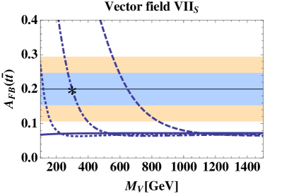
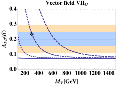
We entertain the possibility that AFBtt¯superscriptsubscript𝐴𝐹𝐵𝑡¯𝑡A_{FB}^{t\bar{t}} is enhanced above SM levels via tree level exchanges of flavor symmetric scalars or vectors. The experimental evidence for such enhancement is as follows. Using 5.3fb15.3superscriptfb15.3{\rm fb}^{-1} of data CDF measured an inclusive asymmetry AFBtt¯=0.158±0.072±0.017superscriptsubscript𝐴𝐹𝐵𝑡¯𝑡plus-or-minus0.1580.0720.017A_{FB}^{t\bar{t}}=0.158\pm 0.072\pm 0.017 in the tt¯𝑡¯𝑡t\,\bar{t} rest frame (fixing mt=172.5GeVsubscript𝑚𝑡172.5GeVm_{t}=172.5\,{\rm GeV}Aaltonen:2011kc . In a channel with both t𝑡t and t¯¯𝑡\bar{t} decaying semileptonically an even larger asymmetry was found, AFBtt¯=0.42±0.15±0.05superscriptsubscript𝐴𝐹𝐵𝑡¯𝑡plus-or-minus0.420.150.05A_{FB}^{t\bar{t}}=0.42\pm 0.15\pm 0.05 CDF-dilepton . Similarly, a recent DØ  analysis finds AFBtt¯=0.196±0.0600.026+0.018superscriptsubscript𝐴𝐹𝐵𝑡¯𝑡plus-or-minus0.196subscriptsuperscript0.0600.0180.026A_{FB}^{t\bar{t}}=0.196\pm 0.060^{+0.018}_{-0.026} using 5.4fb15.4superscriptfb15.4{\rm fb}^{-1} of data  Abazov:2011rq . Combining in quadrature the statistical and systematic errors of the three measurements gives AFBtt¯=0.200±0.047superscriptsubscript𝐴𝐹𝐵𝑡¯𝑡plus-or-minus0.2000.047A_{FB}^{t\bar{t}}=0.200\pm 0.047. This is to be compared to the SM prediction AFBtt¯,SM=0.0720.007+0.011superscriptsubscript𝐴𝐹𝐵𝑡¯𝑡𝑆𝑀subscriptsuperscript0.0720.0110.007A_{FB}^{t\bar{t},SM}=0.072^{+0.011}_{-0.007} from an approximate NNLO QCD calculation Ahrens:2011uf with mt=173.1GeVsubscript𝑚𝑡173.1GeVm_{t}=173.1\,{\rm GeV} and using the MSTW2008 set of PDFs Martin:2009iq . Inclusion of electroweak corrections leads to an enhancement of the asymmetry, with AFBtt¯,SM=0.09±0.01superscriptsubscript𝐴𝐹𝐵𝑡¯𝑡𝑆𝑀plus-or-minus0.090.01A_{FB}^{t\bar{t},SM}=0.09\pm 0.01 recently obtained in Ref. Hollik:2011ps . In the pp¯𝑝¯𝑝p\bar{p} frame, a recent approximate NNLO calculation Kidonakis:2011zn gives AFBtt¯SM=0.0520.006+0.000superscriptsubscript𝐴𝐹𝐵𝑡¯𝑡𝑆𝑀subscriptsuperscript0.0520.0000.006A_{FB}^{t\bar{t}\,SM}=0.052^{+0.000}_{-0.006} with mt=173GeVsubscript𝑚𝑡173GeVm_{t}=173\,{\rm GeV}, to be compared with the CDF value of AFBtt¯=0.150±0.058±0.024superscriptsubscript𝐴𝐹𝐵𝑡¯𝑡plus-or-minus0.1500.0580.024A_{FB}^{t\bar{t}}=0.150\pm 0.058\pm 0.024 Aaltonen:2011kc . The approximate NNLO SM predictions use the known NLO results Antunano:2007da ; Bowen:2005ap ; Kuhn:1998kw and build on recent progress in NNLO calculations Moch:2008ai ; Czakon:2009zw ; Beneke:2009ye ; Kidonakis:2008mu ; Cacciari:2008zb ; Kidonakis:2010dk . DØ  also reports a leptonic asymmetry AFBl=0.152±0.0380.013+0.010superscriptsubscript𝐴𝐹𝐵𝑙plus-or-minus0.152subscriptsuperscript0.0380.0100.013A_{FB}^{l}=0.152\pm 0.038^{+0.010}_{-0.013} to be compared to the MC@NLO prediction of AFBl,SM=0.021±0.001superscriptsubscript𝐴𝐹𝐵𝑙SMplus-or-minus0.0210.001A_{FB}^{l,\rm SM}=0.021\pm 0.001 Abazov:2011rq .

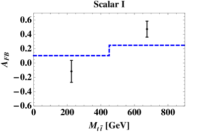
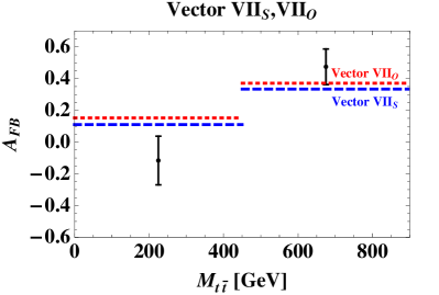
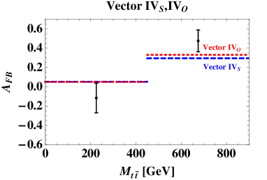
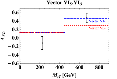
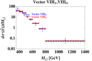
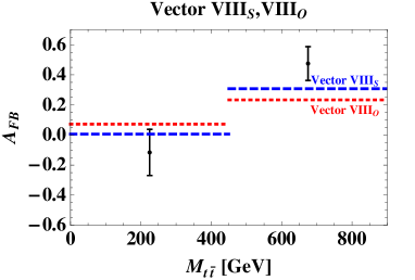
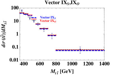
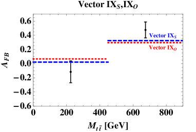
CDF reported evidence that the anomalously large asymmetry rises with the invariant mass of the tt¯𝑡¯𝑡t\,\bar{t} system, with AFBtt¯(Mtt¯>450GeV)=0.475±0.114superscriptsubscript𝐴𝐹𝐵𝑡¯𝑡subscript𝑀𝑡¯𝑡450GeVplus-or-minus0.4750.114A_{FB}^{t\bar{t}}(M_{t\bar{t}}>450{\rm~{}GeV})=0.475\pm 0.114, while AFBtt¯(Mtt¯<450GeV)=0.116±0.153superscriptsubscript𝐴𝐹𝐵𝑡¯𝑡subscript𝑀𝑡¯𝑡450GeVplus-or-minus0.1160.153A_{FB}^{t\bar{t}}(M_{t\bar{t}}<450{\rm~{}GeV})=-0.116\pm 0.153 Aaltonen:2011kc . A similar rise of the asymmetry with respect to the absolute top vs. anti-top rapidity difference |Δy|=|ytyt¯|Δ𝑦subscript𝑦𝑡subscript𝑦¯𝑡|\Delta y|=|y_{t}-y_{\bar{t}}| was also reported by CDF with AFBtt¯(|Δy|<1.0)=0.026±0.104±0.056superscriptsubscript𝐴𝐹𝐵𝑡¯𝑡Δ𝑦1.0plus-or-minus0.0260.1040.056A_{FB}^{t\bar{t}}(|\Delta y|<1.0)=0.026\pm 0.104\pm 0.056 and AFBtt¯(|Δy|>1.0)=0.611±0.210±0.147superscriptsubscript𝐴𝐹𝐵𝑡¯𝑡Δ𝑦1.0plus-or-minus0.6110.2100.147A_{FB}^{t\bar{t}}(|\Delta y|>1.0)=0.611\pm 0.210\pm 0.147 Aaltonen:2011kc . The recent DØ  analysis Abazov:2011rq does not observe a significant rise of the “folded” detector level asymmetry with respect to Mtt¯subscript𝑀𝑡¯𝑡M_{t\bar{t}} and |Δy|Δ𝑦|\Delta y|. However, until these results are unfolded they can not be directly compared to the CDF measurements, although at the detector level they appear to be consistent within errors. We collect the above results in Table 3.

Observable Measurement SM predict.
AFBtt¯superscriptsubscript𝐴𝐹𝐵𝑡¯𝑡A_{FB}^{t\bar{t}} 0.158±0.072±0.017Aaltonen:2011kc 0.42±0.15±0.05CDF-dilepton 0.196±0.0600.026+0.018Abazov:2011rq }0.200±0.047\left.\begin{matrix}0.158\pm 0.072\pm 0.017\,\text{\cite[cite]{\@@bibref{Authors Phrase1YearPhrase2}{Aaltonen:2011kc}{\@@citephrase{(}}{\@@citephrase{)}}}}\\ 0.42\pm 0.15\pm 0.05\,\text{\cite[cite]{\@@bibref{Authors Phrase1YearPhrase2}{CDF-dilepton}{\@@citephrase{(}}{\@@citephrase{)}}}}\\ 0.196\pm 0.060^{+0.018}_{-0.026}\,\text{\cite[cite]{\@@bibref{Authors Phrase1YearPhrase2}{Abazov:2011rq}{\@@citephrase{(}}{\@@citephrase{)}}}}\\ \end{matrix}\right\}\simeq 0.200\pm 0.047 (7.240.67+1.04)0.27+0.20102Ahrens:2011uf (7.24^{+1.04}_{-0.67}{}^{+0.20}_{-0.27})\cdot 10^{-2}\text{\cite[cite]{\@@bibref{Authors Phrase1YearPhrase2}{Ahrens:2011uf}{\@@citephrase{(}}{\@@citephrase{)}}}}
AFBtt¯(Mtt¯>450A_{FB}^{t\bar{t}}(M_{t\bar{t}}>450GeV) 0.475±0.101±0.049plus-or-minus0.4750.1010.0490.475\pm 0.101\pm 0.049 Aaltonen:2011kc (11.10.9+1.7)102Ahrens:2011uf subscriptsuperscript11.11.70.9superscript102Ahrens:2011uf (11.1^{+1.7}_{-0.9})\cdot 10^{-2}\text{\cite[cite]{\@@bibref{Authors Phrase1YearPhrase2}{Ahrens:2011uf}{\@@citephrase{(}}{\@@citephrase{)}}}}
AFBtt¯(Mtt¯<450A_{FB}^{t\bar{t}}(M_{t\bar{t}}<450GeV) 0.116±0.146±0.047plus-or-minus0.1160.1460.047-0.116\pm 0.146\pm 0.047 Aaltonen:2011kc (5.20.6+0.9)102subscriptsuperscript5.20.90.6superscript102(5.2^{+0.9}_{-0.6})\cdot 10^{-2} Ahrens:2011uf
AFBtt¯(|Δy|<1.0A_{FB}^{t\bar{t}}(|\Delta y|<1.0) 0.026±0.104±0.056plus-or-minus0.0260.1040.0560.026\pm 0.104\pm 0.056 Aaltonen:2011kc (4.770.35+0.39)102subscriptsuperscript4.770.390.35superscript102(4.77^{+0.39}_{-0.35})\cdot 10^{-2} Ahrens:2011uf
AFBtt¯(|Δy|>1.0A_{FB}^{t\bar{t}}(|\Delta y|>1.0) 0.611±0.210±0.147plus-or-minus0.6110.2100.1470.611\pm 0.210\pm 0.147 Aaltonen:2011kc (14.591.30+2.16)102subscriptsuperscript14.592.161.30superscript102(14.59^{+2.16}_{-1.30})\cdot 10^{-2} Ahrens:2011uf
σtt¯subscript𝜎𝑡¯𝑡\sigma_{t\bar{t}} (6.9±1.0)plus-or-minus6.91.0(6.9\pm 1.0)pb Aaltonen:2009iz {(6.630.27+0.00)pb Ahrens:2011mw (7.080.24+0.00)0.27+0.36pb Kidonakis:2011jg \left\{\begin{matrix}(6.63^{+0.00}_{-0.27})\text{pb \cite[cite]{\@@bibref{Authors Phrase1YearPhrase2}{Ahrens:2011mw}{\@@citephrase{(}}{\@@citephrase{)}}}}\\ (7.08^{+0.00}_{-0.24}{}^{+0.36}_{-0.27})\text{pb \cite[cite]{\@@bibref{Authors Phrase1YearPhrase2}{Kidonakis:2011jg}{\@@citephrase{(}}{\@@citephrase{)}}}}\end{matrix}\right.
Table 3: Measurements and predictions for observables in tt¯𝑡¯𝑡t\bar{t} production at the Tevatron. We quote the approximate NNLO QCD prediction of AFBtt¯superscriptsubscript𝐴𝐹𝐵𝑡¯𝑡A_{FB}^{t\,\bar{t}} from Ahrens:2011uf using MSTW2008 PDFs Martin:2009iq . The two other choices for PDFs give results in agreement with these Ahrens:2011uf . Among the cross section predictions obtained in Ahrens:2011mw we quote the 1PISCET1PsubscriptISCET{\rm 1PI}_{\rm SCET} one.

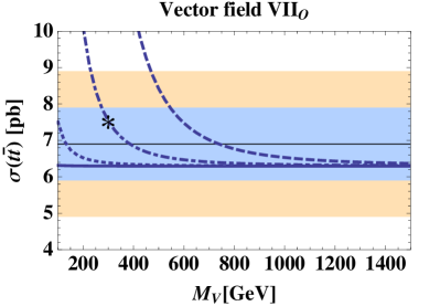
Any NP enhancement of AFBtt¯superscriptsubscript𝐴𝐹𝐵𝑡¯𝑡A_{FB}^{t\bar{t}} must not spoil the agreement between the measured production cross section, σ^tt¯subscript^𝜎𝑡¯𝑡\hat{\sigma}_{t\,\bar{t}}, and the SM predictions. At NLO with NNLL summation of threshold logarithms, the SM prediction is σtt¯=(6.630.27+0.00)subscript𝜎𝑡¯𝑡subscriptsuperscript6.630.000.27\sigma_{t\bar{t}}=(6.63^{+0.00}_{-0.27})pb Ahrens:2011mw (using MSTW2008 pdf sets and 1PISCET1PsubscriptISCET{\rm 1PI_{SCET}} choice of kinematic variables and resummations – the other choices give consistent results but with larger error bars). This is somewhat smaller than the approximate NNLO result (for mt=173GeVsubscript𝑚𝑡173GeVm_{t}=173\,\,{\rm GeV}), σtt¯=7.080.24+0.000.27+0.36\sigma_{t\bar{t}}=7.08^{+0.00}_{-0.24}{}^{+0.36}_{-0.27} pb Kidonakis:2011jg (see also Cacciari:2008zb ; Kidonakis:2008mu ; Moch:2008ai ). Both of these results agree well, within errors, with the measured CDF result based on 4.6fb14.6𝑓superscript𝑏14.6fb^{-1} of data Aaltonen:2009iz σtt¯(mt=173.1GeV)=6.9±1.0pbsubscript𝜎𝑡¯𝑡subscript𝑚𝑡173.1GeVplus-or-minus6.91.0pb\sigma_{t\,\bar{t}}(m_{t}=173.1\,{\rm GeV})=6.9\pm 1.0{\rm pb}. Thus the NP contribution to the tt¯𝑡¯𝑡t\bar{t} cross section, σtt¯NPsuperscriptsubscript𝜎𝑡¯𝑡NP\sigma_{t\,\bar{t}}^{\rm NP}, is tightly constrained.

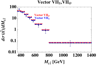
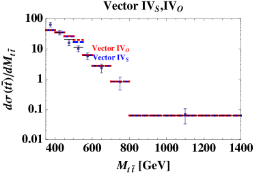
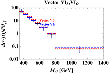
Good agreement between experiment and SM predictions is also seen in the differential cross section dσ/dMtt¯𝑑𝜎𝑑subscript𝑀𝑡¯𝑡d\sigma/dM_{t\bar{t}}. This has important implications for the viability of different NP models. For instance, comparing the measured and predicted cross sections together with the measured and predicted AFBtt¯superscriptsubscript𝐴𝐹𝐵𝑡¯𝑡A_{FB}^{t\bar{t}}, for Mtt¯>450subscript𝑀𝑡¯𝑡450M_{t\bar{t}}>450 GeV, one finds that the NP contributions need to reduce the backward tt¯𝑡¯𝑡t\bar{t}-scattering cross section (a statement valid at 2σ2𝜎2\sigma). This can only happen if NP interferes with the SM Grinstein:2011yv . NP in the s𝑠s-channel which interferes with the single gluon exchange amplitude must therefore be due to color octet fields. In general s𝑠s-channel resonances lead to significant effects in dσ/dMtt¯𝑑𝜎𝑑subscript𝑀𝑡¯𝑡d\sigma/dM_{t\,\bar{t}}. However, this may be avoided for a purely axial gluon that is broad Tavares:2011zg , in particular regions of parameter space. There are no such clear requirements on the charge assignments of possible t𝑡t-channel NP contributions. However, a characteristic high mass tail in the spectrum could lead to tension with the Tevatron and future LHC cross section measurements at large Mtt¯subscript𝑀𝑡¯𝑡M_{t\bar{t}}.

We collect expressions to be used in our analysis below. The total cross section σtt¯subscript𝜎𝑡¯𝑡\sigma_{t\,\bar{t}}, forward-backward asymmetry AFBtt¯superscriptsubscript𝐴𝐹𝐵𝑡¯𝑡A_{FB}^{t\bar{t}}, and the cross sections for forward and backward scattering σF,Bsubscript𝜎𝐹𝐵\sigma_{F,B} are defined as

σtt¯=σF+σB,AFBtt¯=σFσBσF+σB,σF(B)=0(1)1(0)dcosθdσdcosθ,formulae-sequencesubscript𝜎𝑡¯𝑡subscript𝜎𝐹subscript𝜎𝐵formulae-sequencesuperscriptsubscript𝐴𝐹𝐵𝑡¯𝑡subscript𝜎𝐹subscript𝜎𝐵subscript𝜎𝐹subscript𝜎𝐵subscript𝜎𝐹𝐵superscriptsubscript0110𝑑𝜃𝑑𝜎𝑑𝜃\sigma_{t\,\bar{t}}=\sigma_{F}+\sigma_{B},\qquad A_{FB}^{t\bar{t}}=\frac{\sigma_{F}-\sigma_{B}}{\sigma_{F}+\sigma_{B}},\qquad\sigma_{F(B)}=\int_{0(-1)}^{1(0)}d\cos\theta\,\frac{d\sigma}{d\cos\theta}, (13)

where θ𝜃\theta is the angle between incoming proton and outgoing top quark. We use NLO SM predictions for σtt¯subscript𝜎𝑡¯𝑡\sigma_{t\,\bar{t}} and dσtt¯/dMtt¯𝑑subscript𝜎𝑡¯𝑡𝑑subscript𝑀𝑡¯𝑡d\sigma_{t\,\bar{t}}/dM_{t\bar{t}}, and LO predictions for the NP corrections (including interference with the SM). To obtain AFBtt¯superscriptsubscript𝐴𝐹𝐵𝑡¯𝑡A_{FB}^{t\bar{t}} we define a partonic level asymmetry,

AFBNP+SM=σFNPσBNP(σFNP+SM)LO+(σBNP+SM)LO+AFBSM(σSMσSM+σNP),superscriptsubscript𝐴𝐹𝐵𝑁𝑃𝑆𝑀subscriptsuperscript𝜎𝑁𝑃𝐹subscriptsuperscript𝜎𝑁𝑃𝐵subscriptsubscriptsuperscript𝜎NPSM𝐹𝐿𝑂subscriptsubscriptsuperscript𝜎NPSM𝐵𝐿𝑂superscriptsubscript𝐴𝐹𝐵𝑆𝑀superscript𝜎𝑆𝑀superscript𝜎𝑆𝑀superscript𝜎𝑁𝑃\displaystyle A_{FB}^{NP+SM}=\frac{\sigma^{NP}_{F}-\sigma^{NP}_{B}}{(\sigma^{\rm NP+SM}_{F})_{LO}+(\sigma^{\rm NP+SM}_{B})_{LO}}+A_{FB}^{SM}\left(\frac{\sigma^{SM}}{\sigma^{SM}+\sigma^{NP}}\right), (14)

which is to be compared against the binned unfolded partonic level results of Aaltonen:2011kc . We use the NLO + NNLL SM predictions for the forward, backward and total cross sections Ahrens:2010zv , the tt¯𝑡¯𝑡t\bar{t} spectrum Ahrens:2010zv and AFBtt¯,SMsuperscriptsubscript𝐴𝐹𝐵𝑡¯𝑡𝑆𝑀A_{FB}^{t\bar{t},SM} Ahrens:2011uf . For concreteness, for Mtt¯<450subscript𝑀𝑡¯𝑡450M_{t\,\bar{t}}<450 GeV we take the central values σSM=4.23superscript𝜎𝑆𝑀4.23\sigma^{SM}=4.23 pb and AFBtt¯,SM=0.052superscriptsubscript𝐴𝐹𝐵𝑡¯𝑡𝑆𝑀0.052A_{FB}^{t\bar{t},SM}=0.052, while for Mtt¯>450subscript𝑀𝑡¯𝑡450M_{t\,\bar{t}}>450 GeV we take σSM=2.40superscript𝜎𝑆𝑀2.40\sigma^{SM}=2.40 pb and AFBtt¯,SM=0.111superscriptsubscript𝐴𝐹𝐵𝑡¯𝑡𝑆𝑀0.111A_{FB}^{t\bar{t},SM}=0.111 (MSTW08 pdfs); for the inclusive asymmetry (in the tt¯𝑡¯𝑡t\bar{t} rest frame) we take AFBtt¯=0.0724superscriptsubscript𝐴𝐹𝐵𝑡¯𝑡0.0724A_{FB}^{t\bar{t}}=0.0724.

III.1.1 Acceptance effects

As pointed out in Gresham:2011pa ; Jung:2011zv , care is needed when comparing NP predictions to the experimental parton level AFBtt¯superscriptsubscript𝐴𝐹𝐵𝑡¯𝑡A_{FB}^{t\bar{t}} and Mtt¯subscript𝑀𝑡¯𝑡M_{t\bar{t}} differential spectrum deduced by CDF Aaltonen:2009iz ; Aaltonen:2011kc , since the deconvolution was done assuming the SM. The acceptance corrections are especially important if NP enhances top production in the very forward region This is because the SM tt¯𝑡¯𝑡t\bar{t} event distribution is more central. We take into account the CDF experimental cuts using correction factors ϵisubscriptitalic-ϵ𝑖\epsilon_{i}. For the ilimit-from𝑖i-th bin in Mtt¯subscript𝑀𝑡¯𝑡M_{t\bar{t}} one needs to multiply the calculated partonic tt¯𝑡¯𝑡t\bar{t} cross section dσNP/dMtt¯𝑑superscript𝜎NP𝑑subscript𝑀𝑡¯𝑡d\sigma^{\rm NP}/dM_{t\bar{t}} by ϵisubscriptitalic-ϵ𝑖\epsilon_{i} in order to compare with the CDF measured partonic cross section (dσNP/dMtt¯)CDFsuperscript𝑑superscript𝜎NP𝑑subscript𝑀𝑡¯𝑡CDF(d\sigma^{\rm NP}/dM_{t\bar{t}})^{\rm CDF}

(dσNPdMtt¯)iCDF=ϵi×(dσNPdMtt¯)i.subscriptsuperscript𝑑superscript𝜎NP𝑑subscript𝑀𝑡¯𝑡CDF𝑖subscriptitalic-ϵ𝑖subscript𝑑superscript𝜎NP𝑑subscript𝑀𝑡¯𝑡𝑖\left(\frac{d\sigma^{\rm NP}}{dM_{t\bar{t}}}\right)^{\rm CDF}_{i}=\epsilon_{i}\times\left(\frac{d\sigma^{\rm NP}}{dM_{t\bar{t}}}\right)_{i}. (15)

There is no summation over i𝑖i in this equation. Since CDF is using SM acceptances and no bins in ΔyΔ𝑦\Delta y in the deconvolution of the dσ/dMtt¯𝑑𝜎𝑑subscript𝑀𝑡¯𝑡d\sigma/dM_{t\bar{t}} measurement in Aaltonen:2011kc , the ϵisubscriptitalic-ϵ𝑖\epsilon_{i} are given by the ratio of acceptances for the NP model and the SM

ϵi=ϵiNPϵiSM,subscriptitalic-ϵ𝑖superscriptsubscriptitalic-ϵ𝑖NPsuperscriptsubscriptitalic-ϵ𝑖SM\epsilon_{i}=\frac{\epsilon_{i}^{\rm NP}}{\epsilon_{i}^{\rm SM}}, (16)

where ϵiNP(SM)superscriptsubscriptitalic-ϵ𝑖NPSM\epsilon_{i}^{\rm NP(SM)} are calculated by splitting each i𝑖i-th Mtt¯subscript𝑀𝑡¯𝑡M_{t\bar{t}} bin into j𝑗j bins in Δy=ytyt¯Δ𝑦subscript𝑦𝑡subscript𝑦¯𝑡\Delta y=y_{t}-y_{\bar{t}}

ϵiNP(SM)=jϵijσijNP(SM)jσijNP(SM),superscriptsubscriptitalic-ϵ𝑖NPSMsubscript𝑗subscriptitalic-ϵ𝑖𝑗superscriptsubscript𝜎𝑖𝑗NPSMsubscript𝑗superscriptsubscript𝜎𝑖𝑗NPSM\epsilon_{i}^{\rm NP(SM)}=\frac{\sum_{j}\epsilon_{ij}\sigma_{ij}^{\rm NP(SM)}}{\sum_{j}\sigma_{ij}^{\rm NP(SM)}}, (17)

and the sum is over the bins in ΔyΔ𝑦\Delta y. Here ϵijsubscriptitalic-ϵ𝑖𝑗\epsilon_{ij} is the acceptance for each (Mtt¯,Δy)subscript𝑀𝑡¯𝑡Δ𝑦(M_{t\bar{t}},\Delta y) bin, and σijNP(SM)superscriptsubscript𝜎𝑖𝑗NPSM\sigma_{ij}^{\rm NP(SM)} is the corresponding cross section integrated over the bin. The above expressions are approximate in so far as the bins have finite sizes, and the spill-over of events between different bins is not taken into account. The acceptances are calculated by simulating the partonic tt¯𝑡¯𝑡t-\bar{t} cross section using MadGraph4.4.30 Alwall:2007st , decaying the top quarks in Pythia6.4 Sjostrand:2006za , which also simulates the LO showering and hadronization, and using PGS for detector simulation. The events were read into Mathematica, where the cuts from Aaltonen:2008hc ; Aaltonen:2011kc were implemented. The resulting values for the acceptances ϵijsubscriptitalic-ϵ𝑖𝑗\epsilon_{ij} are collected in Table 4.

Mtt¯subscript𝑀𝑡¯𝑡M_{t\bar{t}} (GeV):/Δy::/\Delta y: 00.600.60-0.6 0.61.20.61.20.6-1.2 1.21.81.21.81.2-1.8 1.82.41.82.41.8-2.4 2.43.02.43.02.4-3.0
350400350400350-400 2.422.422.42 2.232.232.23 - - -
400450400450400-450 3.443.443.44 2.742.742.74 1.951.951.95 - -
450500450500450-500 4.294.294.29 3.323.323.32 1.751.751.75 - -
500550500550500-550 5.255.255.25 3.503.503.50 2.342.342.34 1.181.181.18 -
550600550600550-600 5.615.615.61 4.394.394.39 2.672.672.67 1.151.151.15 -
600700600700600-700 6.596.596.59 4.814.814.81 3.013.013.01 1.091.091.09 0.420.420.42
700800700800700-800 7.387.387.38 6.066.066.06 3.493.493.49 1.341.341.34 0.450.450.45
80014008001400800-1400 6.686.686.68 6.266.266.26 4.304.304.30 1.831.831.83 0.420.420.42
Table 4: Acceptances ϵijsubscriptitalic-ϵ𝑖𝑗\epsilon_{ij} (in %) to be used for emulating the CDF deconvolution to parton level measurements (cf. eqs. (15) - (17)). Note that the ϵijsubscriptitalic-ϵ𝑖𝑗\epsilon_{ij} do not depend on the NP model and are symmetric in ΔyΔyΔ𝑦Δ𝑦\Delta y\leftrightarrow-\Delta y.
Refer to caption
Refer to caption
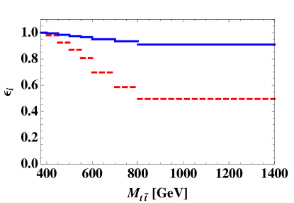
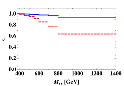
Figure 1: The correction factors ϵisubscriptitalic-ϵ𝑖\epsilon_{i} for t𝑡t-channel dominated vector models VIssubscriptVIs{\rm VI_{s}} (left) and VIosubscriptVIo{\rm VI_{o}} (right), where (mV,ηijη33,ηi3,ΓV/mVsubscript𝑚𝑉subscript𝜂𝑖𝑗subscript𝜂33subscript𝜂𝑖3subscriptΓ𝑉subscript𝑚𝑉m_{V},\sqrt{\eta_{ij}\eta_{33}},\eta_{i3},\Gamma_{V}/m_{V})=(300GeV,1,1.33,0.08300GeV11.330.08300\,{\rm GeV},1,1.33,0.08)[dashed red]; (1200GeV,2.2,4.88,0.51200GeV2.24.880.51200\,{\rm GeV},2.2,4.88,0.5)[solid blue].

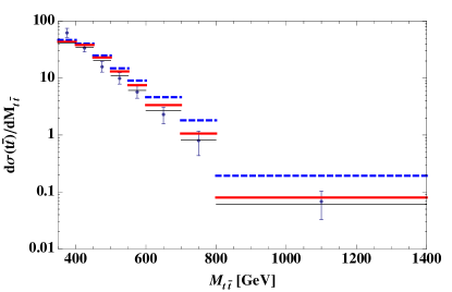
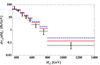
In Fig. 1 the correction factors ϵisubscriptitalic-ϵ𝑖\epsilon_{i} are shown as a function of the Mtt¯subscript𝑀𝑡¯𝑡M_{t\bar{t}} bin for two benchmarks points (corresponding to illustrative couplings and mass valuers) in models VIs,osubscriptVIso{\rm VI_{s,o}} which exhibit substantial departures from the SM acceptances. Results for dσ/dMtt¯𝑑𝜎𝑑subscript𝑀𝑡¯𝑡d\sigma/dM_{t\bar{t}} and AFBtt¯superscriptsubscript𝐴𝐹𝐵𝑡¯𝑡A_{FB}^{t\bar{t}} for the two model VIosubscriptVIo\rm VI_{o} benchmark points in Fig. 1 were shown previously without acceptance corrections Grinstein:2011yv . The differential distributions with acceptance corrections are compared to those in  Grinstein:2011yv in Fig. 2. We see that the corrections bring the predicted spectrum for the light vector example into good agreement with experiment. For the remaining GFsubscriptGF\rm G_{F} representations discussed below, the correction factors are not as important. For models SVsubscriptSV\rm S_{V}, VIIIssubscriptVIIIs{\rm VIII_{s}} and IXssubscriptIXs{\rm IX_{s}} the ϵisubscriptitalic-ϵ𝑖\epsilon_{i} are below 15%percent1515\%, and for the others they are below 5%percent55\%, for all Mtt¯subscript𝑀𝑡¯𝑡M_{t\bar{t}} bins and all benchmarks points considered.

The pattern of acceptance corrections ϵisubscriptitalic-ϵ𝑖\epsilon_{i} can be understood from the angular dependence of the NP contribution to the differential cross section in each model. For instance, the t𝑡t-channel exchange of a vector with mass mVsubscript𝑚𝑉m_{V} leads to a Rutherford scattering peak in the forward direction for mtt¯2>>mV2much-greater-thansubscriptsuperscript𝑚2𝑡¯𝑡subscriptsuperscript𝑚2𝑉m^{2}_{t\bar{t}}>>m^{2}_{V}. Specifically, the expressions for the NP cross sections contain characteristic t𝑡t-channel (1cosθ)2,4superscript1𝜃24(1-\cos\theta)^{2,4} factors in the denominators, whose angular dependence is reinforced by (1+cosθ)2superscript1𝜃2(1+\cos\theta)^{2} factors in the numerators, where θ𝜃\theta is the top quark scattering angle in the tt¯𝑡¯𝑡t\bar{t} center of mass frame. Thus, models VIs,osubscriptVIso{\rm VI_{s,o}} with light vector masses favor forward top-quark production at large Mtt¯subscript𝑀𝑡¯𝑡M_{t\bar{t}}, yielding ϵisubscriptitalic-ϵ𝑖\epsilon_{i} that are substantially less than 1 in the high Mtt¯subscript𝑀𝑡¯𝑡M_{t\bar{t}} bins. In models SIsubscriptSI\rm S_{I} (t𝑡t-channel) and SVsubscriptSV\rm S_{V}, SVIsubscriptSVI\rm S_{VI} (u𝑢u-channel), the angular dependence introduced by the characteristic (1cosθ)2,4superscriptminus-or-plus1𝜃24(1\mp\cos\theta)^{2,4} factors in the denominators is offset by (1cosθ)2superscriptminus-or-plus1𝜃2(1\mp\cos\theta)^{2} factors in the numerators, which leads to central NP top-quark production, as in the SM. The result is that the ϵisubscriptitalic-ϵ𝑖\epsilon_{i} in these models are actually slightly larger than 1.

To apply the acceptance corrections to AFBtt¯superscriptsubscript𝐴𝐹𝐵𝑡¯𝑡A_{FB}^{t\bar{t}} we follow CDF, where AFBtt¯superscriptsubscript𝐴𝐹𝐵𝑡¯𝑡A_{FB}^{t\bar{t}} was obtained using four bins in Mtt¯subscript𝑀𝑡¯𝑡M_{t\bar{t}} and ΔyΔ𝑦\Delta y: Mtt¯subscript𝑀𝑡¯𝑡M_{t\bar{t}} above or below 450450450 GeV and ΔyΔ𝑦\Delta y positive or negative. The correction factor for each of the four bins is given as in Eqs. (15)-(17), except that the sum in (17) now runs over all j𝑗j with either Δy>0Δ𝑦0\Delta y>0 or Δy<0Δ𝑦0\Delta y<0, and over the appropriate values of i𝑖i with either Mtt¯>450subscript𝑀𝑡¯𝑡450M_{t\bar{t}}>450 GeV or Mtt¯<450subscript𝑀𝑡¯𝑡450M_{t\bar{t}}<450 GeV. We find that the corrections are small for all of the models we consider. For instance, for the light vector color octet example in Fig. 1 the shift is from an uncorrected AFBtt¯=(0.10949,0.357)superscriptsubscript𝐴𝐹𝐵𝑡¯𝑡0.109490.357A_{FB}^{t\bar{t}}=(0.10949,0.357) to a corrected AFBtt¯=(0.10953,0.339)superscriptsubscript𝐴𝐹𝐵𝑡¯𝑡0.109530.339A_{FB}^{t\bar{t}}=(0.10953,0.339), where the first and second numbers are the low and high mass bins in AFBtt¯superscriptsubscript𝐴𝐹𝐵𝑡¯𝑡A_{FB}^{t\bar{t}}. The small shifts in AFBtt¯superscriptsubscript𝐴𝐹𝐵𝑡¯𝑡A_{FB}^{t\bar{t}} are due to the coarse binning in Mtt¯subscript𝑀𝑡¯𝑡M_{t\bar{t}} Gresham:2011pa . In particular, the high mass bin is dominated by events with Mtt¯subscript𝑀𝑡¯𝑡M_{t\bar{t}} near 450 GeV, which are more central, as in the SM.
Refer to captionRefer to caption

Figure 2: The effect of acceptance corrections on the vector model discussed in Grinstein:2011yv . Before acceptance corrections (left), after corrections applied (right). For the parameters (mV,ηijη33,ηi3,ΓV/mVsubscript𝑚𝑉subscript𝜂𝑖𝑗subscript𝜂33subscript𝜂𝑖3subscriptΓ𝑉subscript𝑚𝑉m_{V},\sqrt{\eta_{ij}\eta_{33}},\eta_{i3},\Gamma_{V}/m_{V}): solid red (300GeV,1,1.33,0.08300GeV11.330.08300\,{\rm GeV},1,1.33,0.08); dashed blue (1200GeV,2.2,4.88,0.51200GeV2.24.880.51200\,{\rm GeV},2.2,4.88,0.5).

III.1.2 The tt¯𝑡¯𝑡t\,\bar{t} phenomenology of HFsubscriptHF\rm H_{F} symmetric scalar fields

The flavor symmetric models introduced in Section II and collected in Tables 1, 2 can couple to light and heavy quark bilinears with unsuppressed couplings. They are thus interesting candidates to explain the AFBtt¯superscriptsubscript𝐴𝐹𝐵𝑡¯𝑡A_{FB}^{t\bar{t}} anomaly, as noted in Arnold:2009ay ; Grinstein:2011yv ; Ligeti:2011vt . In the case of scalars, SU(2)LSUsubscript2L\rm SU(2)_{L} singlet color triplets or color sextets and SU(2)LSUsubscript2L\rm SU(2)_{L} doublet color singlets have previously been identified as being promising for explaining the AFBtt¯superscriptsubscript𝐴𝐹𝐵𝑡¯𝑡A_{FB}^{t\bar{t}} anomaly Shu:2009xf ; Grinstein:2011yv ; Ligeti:2011vt ; Nelson:2011us ; Babu:2011yw ; AguilarSaavedra:2011hz ; Blum:2011fa . Here, we will focus on some of the flavored versions listed in Table 2. Our results overlap with past studies, but we also include color triplet and sextet scalars that couple to initial state down quarks, that have not been studied as extensively. We find that these models may also be viable, although they generically require a coupling that is a factor of 2similar-toabsent2\sim 2 larger than if the up quark is in the initial state. This rule of thumb also holds for the vector models that we will study in next subsection.
Refer to caption
Refer to caption
Refer to caption
Refer to caption
Refer to caption
Refer to caption
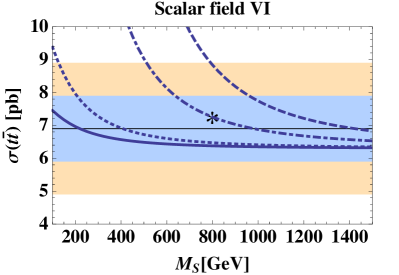
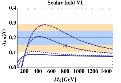
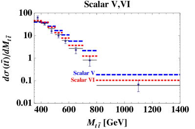
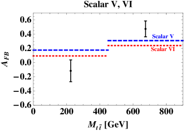
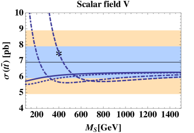
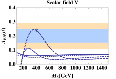
Figure 3: Upper two rows: predictions for the inclusive cross sections σ(tt¯)𝜎𝑡¯𝑡\sigma(t\bar{t}) and inclusive forward-backward asymmetry AFB(tt¯)subscript𝐴𝐹𝐵𝑡¯𝑡A_{FB}(t\bar{t}) as a function of scalar mass mSsubscript𝑚𝑆m_{S} for models SV,SVIsubscriptSVsubscriptSVI\rm S_{V},S_{VI} and couplings η=1/4𝜂14\eta=1/4 (solid line), 1/221221/2\sqrt{2} (dotted), 1/2121/\sqrt{2} (dot-dashed), 111 (dashed) compared to 1σ1𝜎1\sigma and 2σ2𝜎2\sigma experimental (shaded) bands. Predictions for AFBtt¯superscriptsubscript𝐴𝐹𝐵𝑡¯𝑡A_{FB}^{t\bar{t}} with Mtt¯subscript𝑀𝑡¯𝑡M_{t\bar{t}} below and above 450 GeV and for dσtt¯/dMtt¯𝑑subscript𝜎𝑡¯𝑡𝑑subscript𝑀𝑡¯𝑡d\sigma_{t\,\bar{t}}/dM_{t\,\bar{t}} are compared to the experimental data from Aaltonen:2009iz ; Aaltonen:2011kc in the last row for benchmark points labeled with a \star in the inclusive predictions (mS=400subscript𝑚𝑆400m_{S}=400 GeV for SVsubscriptSV\rm S_{V} and 800 GeV for SVIsubscriptSVI\rm S_{VI}).

We show results below for models SV,VIsubscriptSVVI\rm S_{V,VI} that couple to initial state up quarks, for models SIX,XsubscriptSIXX\rm S_{IX,X} that couple to initial state down quarks, and model SIsubscriptSI\rm S_{I} that couples to initial state up and down quarks. (Flavored color sextets and color triplets were considered previously in Grinstein:2011yv ; Ligeti:2011vt ). We expect models SXISXIVsubscriptSXIsubscriptSXIV\rm S_{XI}-S_{XIV} to yield results similar to those for SIX,SXsubscriptSIXsubscriptSX\rm S_{IX},S_{X}. The scalar models SIIIsubscriptSIII{\rm S_{III}} and SIVsubscriptSIV{\rm S_{IV}} are in the 𝟏1\bf 1 and 𝟖8\bf 8 color representations respectively. These models are known to generically suppress AFBtt¯superscriptsubscript𝐴𝐹𝐵𝑡¯𝑡A_{FB}^{t\bar{t}} when interfering with the SM Shu:2009xf and we do not consider them further.

The interaction Lagrangians for scalar models SIsubscriptSI\rm S_{I} and SIXsubscriptSIX\rm S_{IX} are

IsubscriptI\displaystyle{\cal L}_{\rm I} =η(Sij0u¯iLujR+Sijd¯iLujR)+h.c.,formulae-sequenceabsent𝜂subscriptsuperscript𝑆0𝑖𝑗subscript¯𝑢𝑖𝐿subscript𝑢𝑗𝑅superscriptsubscript𝑆𝑖𝑗subscript¯𝑑𝑖𝐿subscript𝑢𝑗𝑅𝑐\displaystyle=\eta\,(\,S^{0}_{ij}\bar{u}_{i\,L}u_{j\,R}+S_{ij}^{-}\bar{d}_{i\,L}u_{j\,R})+h.c., (18)
IXsubscriptIX\displaystyle{\cal L}_{\rm IX} =ηϵαβγSijαdRiβuRjγ+h.c.,formulae-sequenceabsent𝜂subscriptitalic-ϵ𝛼𝛽𝛾superscriptsubscript𝑆𝑖𝑗𝛼superscriptsubscript𝑑𝑅𝑖𝛽superscriptsubscript𝑢𝑅𝑗𝛾𝑐\displaystyle=\eta\,\epsilon_{\alpha\beta\gamma}S_{ij}^{\alpha}d_{R}^{\,i\,\beta}\,u_{R}^{\,j\,\gamma}~{}+~{}h.c., (19)

where i,j𝑖𝑗i,j and α,β,γ𝛼𝛽𝛾\alpha,\beta,\gamma denote flavor and color indices, respectively. Explicit forms of the interaction Lagrangians for the remaining scalar models under discussion, SV,VI,XsubscriptSVVIX\rm S_{V,VI,X} are collected in Appendix A. In the GFsubscriptGF\rm G_{F} symmetric limit the decay widths of the scalars are κη2mS/16π𝜅superscript𝜂2subscript𝑚𝑆16𝜋\kappa\,\eta^{2}\,m_{S}/16\pi, where η𝜂\eta is the coupling of the scalar field to the SM quarks, and κ=1, 8, 8, 2, 2𝜅18822\kappa=1,\,8,\,8,\,2,\,2 in models SI,SVsubscriptSIsubscriptSV\rm S_{I},S_{V}, SVIsubscriptSVI\rm S_{VI}, SIXsubscriptSIX\rm S_{IX}, SXsubscriptSX\rm S_{X}, respectively (assuming all quark decay channels are open and ignoring phase space effects). The interaction Lagrangians explicitly defining η𝜂\eta are collected in Appendix A, while the relevant NP cross section formulae for top quark pair production can be found in Appendix B.

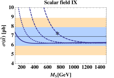
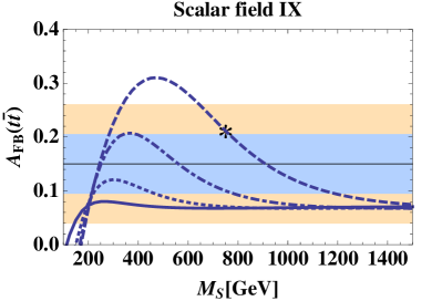
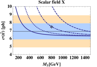
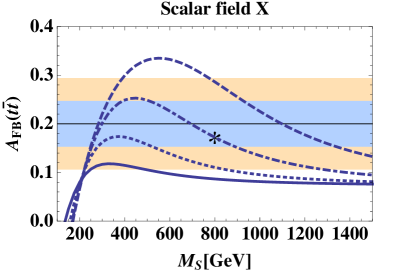
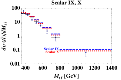
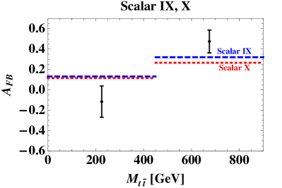
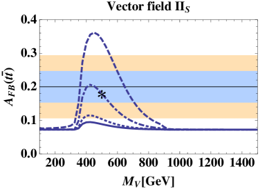
In Figs. 3 and 4 we collect predictions for the inclusive AFBtt¯superscriptsubscript𝐴𝐹𝐵𝑡¯𝑡A_{FB}^{t\bar{t}} and σtt¯subscript𝜎𝑡¯𝑡{\sigma}_{t\,\bar{t}} as functions of the scalar masses in models SVsubscriptSV\rm S_{V}, SVIsubscriptSVI\rm S_{VI}, SIXsubscriptSIX\rm S_{IX}, and SXsubscriptSX\rm S_{X}, for several values of the couplings η𝜂\eta to quarks. These results do not depend on whether one is considering the GFsubscriptGF\rm G_{F} symmetric limits in Eqs. (19), (65), and (66)), or the HFsubscriptHF{\rm H_{F}} symmetric limits (with the couplings of the light quarks to the top identified with the chosen values of η𝜂\eta). Large effects on AFBtt¯superscriptsubscript𝐴𝐹𝐵𝑡¯𝑡A_{FB}^{t\bar{t}} are possible, while remaining within the 2σ2𝜎2\sigma bounds for σtt¯subscript𝜎𝑡¯𝑡{\sigma}_{t\,\bar{t}}. In general 𝒪(1)𝒪1\mathcal{O}(1) couplings η𝜂\eta are required. Therefore, some GFHFsubscriptGFsubscriptHF\rm G_{F}\rightarrow H_{F} flavor breaking will be necessary in order to satisfy the dijet constraints on the couplings to light quark pairs, particularly in models SVIsubscriptSVI\rm S_{VI} and SXsubscriptSX\rm S_{X} (we comment on this further below). For example, recent LHC dijet measurements imply that in model SVIsubscriptSVI\rm S_{VI} the couplings of light quarks to 1similar-toabsent1\sim 1 TeV mass scalars should be <0.1<0.1{~{}\raise 1.49994pt\hbox{$<$}\kern-8.50006pt\lower 3.50006pt\hbox{$\sim$}~{}}0.1, see Section IV.3.

Refer to caption
Refer to caption
Refer to caption
Refer to caption
Refer to caption
Refer to caption
Figure 4: The same as Fig. 3, but for models SX,IXsubscriptSXIX{\rm S_{X,IX}} and couplings η=1/2𝜂12\eta=1/\sqrt{2} (solid line), 111 (dotted), 22\sqrt{2} (dot-dashed), 222 (dashed). Benchmark masses are mS=750subscript𝑚𝑆750m_{S}=750 GeV (SIXsubscriptSIX\rm S_{IX} ) and mS=800subscript𝑚𝑆800m_{S}=800 GeV (SXsubscriptSX\rm S_{X} ).
Refer to caption
Refer to caption
Refer to caption
Refer to caption
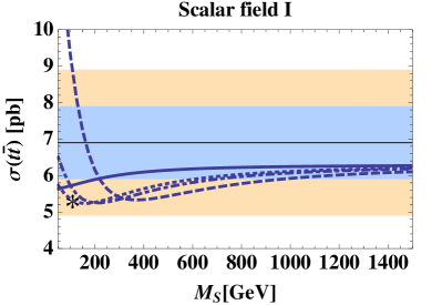
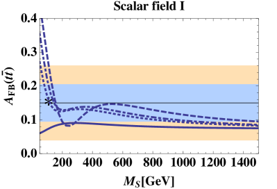
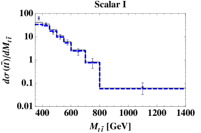
Figure 5: Upper row: predictions for the cross section σ(tt¯)𝜎𝑡¯𝑡\sigma(t\bar{t}) and inclusive forward-backward asymmetry AFB(tt¯)subscript𝐴𝐹𝐵𝑡¯𝑡A_{FB}(t\bar{t}) as a function of scalar mass mSsubscript𝑚𝑆m_{S} for model SIsubscriptSI\rm S_{I} and coupling η=1/3𝜂13\eta=1/3 (solid curve), 2/3232/3 (dotted), 3/4343/4 (dot-dashed), 111 (dashed). Predictions for AFBtt¯subscriptsuperscript𝐴𝑡¯𝑡𝐹𝐵A^{t\bar{t}}_{FB} with Mtt¯subscript𝑀𝑡¯𝑡M_{t\bar{t}} below and above 450 GeV and for dσtt¯/dMtt¯𝑑subscript𝜎𝑡¯𝑡𝑑subscript𝑀𝑡¯𝑡d\sigma_{t\,\bar{t}}/dM_{t\,\bar{t}} are shown in the last row for the benchmark point labeled with a \star in the inclusive predictions (mS=110subscript𝑚𝑆110m_{S}=110 GeV).

A strong constraint on these models is consistency with the measured dσ(tt¯)/dMtt¯𝑑𝜎𝑡¯𝑡𝑑subscript𝑀𝑡¯𝑡d\sigma(t\,\bar{t})/dM_{t\bar{t}} distribution. To demonstrate the potential of these models to explain the AFBtt¯superscriptsubscript𝐴𝐹𝐵𝑡¯𝑡A_{FB}^{t\bar{t}} anomaly and their impact on this spectrum we pick particular benchmark values for the scalar masses and couplings, denoted by a \star in Figs. 3, 4. The resulting dσ(tt¯)/dMtt¯𝑑𝜎𝑡¯𝑡𝑑subscript𝑀𝑡¯𝑡d\sigma(t\,\bar{t})/dM_{t\bar{t}} spectra and AFBtt¯superscriptsubscript𝐴𝐹𝐵𝑡¯𝑡A_{FB}^{t\bar{t}} in the low and high Mtt¯subscript𝑀𝑡¯𝑡M_{t\bar{t}} bins are shown in the last rows of Figs.  3, 4. We do not apply K-factors to the NP cross sections in any of the models we consider. A genuine NLONLO\rm NLO calculation for these models is beyond the scope of this work, but is clearly required before precise conclusions can be drawn regarding the effects of the various models on the dσ/dMtt¯𝑑𝜎𝑑subscript𝑀𝑡¯𝑡d\sigma/dM_{t\bar{t}} distributions. All chosen points predict a significantly enhanced AFBtt¯superscriptsubscript𝐴𝐹𝐵𝑡¯𝑡A_{FB}^{t\bar{t}} in the high invariant mass bin. In general, these models reduce the good agreement between the SM and measured dσ(tt¯)/dMtt¯𝑑𝜎𝑡¯𝑡𝑑subscript𝑀𝑡¯𝑡d\sigma(t\,\bar{t})/dM_{t\bar{t}} spectrum, while improving the agreement in AFBtt¯superscriptsubscript𝐴𝐹𝐵𝑡¯𝑡A_{FB}^{t\bar{t}}. Clearly, there is significant tension between satisfying the constraints on the Mtt¯subscript𝑀𝑡¯𝑡M_{t\bar{t}} distribution while simultaneously creating a large AFBtt¯superscriptsubscript𝐴𝐹𝐵𝑡¯𝑡A_{FB}^{t\bar{t}} enhancement, as has recently been emphasized in Blum:2011fa ; Gresham:2011fx . Recent DØ  data Abazov:2011rq shows a preference for a smaller AFBtt¯subscriptsuperscript𝐴𝑡¯𝑡𝐹𝐵A^{t\bar{t}}_{FB} in the high Mtt¯subscript𝑀𝑡¯𝑡M_{t\bar{t}} bin. While the Mtt¯subscript𝑀𝑡¯𝑡M_{t\bar{t}} dependence of AFBtt¯superscriptsubscript𝐴𝐹𝐵𝑡¯𝑡A_{FB}^{t\bar{t}} has not been unfolded by DØ  , and thus cannot be directly compared to the results in Figs. 3 and 4, some of the tension may be alleviated with the new data.

The flavor breaking naturally present in this framework can reduce the remaining tension with measurements associated with the light quark sector, e.g., from the dijet bounds mentioned above. For instance, keeping the leading insertions in yt2superscriptsubscript𝑦𝑡2y_{t}^{2} that break GFHFsubscriptGFsubscriptHF{\rm G_{F}}\rightarrow{\rm H_{F}}, the Lagrangian for scalar model SIXsubscriptSIX\rm S_{IX} in the mass eigenstate basis becomes,

IX=η1(dR)αi(uR)βjSγi,jϵαβγ+(η1+2η2yt2)(dR)αi(tR)βSγi,3ϵαβγ,subscriptIXsubscript𝜂1subscriptsuperscriptsubscript𝑑𝑅𝛼𝑖subscriptsuperscriptsubscript𝑢𝑅𝛽𝑗superscriptsubscript𝑆𝛾superscript𝑖𝑗superscriptitalic-ϵ𝛼𝛽𝛾subscript𝜂12subscript𝜂2superscriptsubscript𝑦𝑡2subscriptsuperscriptsubscript𝑑𝑅𝛼𝑖subscriptsuperscriptsubscript𝑡𝑅𝛽superscriptsubscript𝑆𝛾superscript𝑖3superscriptitalic-ϵ𝛼𝛽𝛾\displaystyle\mathcal{L}_{\rm IX}=\eta_{1}\,(d_{R}^{\prime})_{\alpha i}\,(u_{R}^{\prime})_{\beta j}\,S_{\gamma}^{{}^{\prime}i,j}\,\epsilon^{\alpha\beta\gamma}+\left(\eta_{1}+2\,\eta_{2}\,y_{t}^{2}\right)(d_{R}^{\prime})_{\alpha i}\,(t_{R}^{\prime})_{\beta}\,S_{\gamma}^{{}^{\prime}i,3}\,\epsilon^{\alpha\beta\gamma}, (20)

with j={1,2}𝑗12j=\{1,2\} and i={1,2,3}𝑖123i=\{1,2,3\}. The mass spectrum is split, with mi32=mij2+ζ~1mS2superscriptsubscript𝑚𝑖32superscriptsubscript𝑚𝑖𝑗2subscript~𝜁1superscriptsubscript𝑚𝑆2m_{i3}^{2}=m_{ij}^{2}+\tilde{\zeta}_{1}m_{S}^{2}. Depending on the signs of η1,2subscript𝜂12\eta_{1,2} and ζ~1subscript~𝜁1\tilde{\zeta}_{1} one can have an enhanced coupling to top quarks (compared to couplings to light quarks) with a suppressed mass scale of the mi32superscriptsubscript𝑚𝑖32m_{i3}^{2} components of the scalar. This can naturally lead to larger effects on top phenomenology, such as AFBtt¯superscriptsubscript𝐴𝐹𝐵𝑡¯𝑡A_{FB}^{t\bar{t}} and σtt¯subscript𝜎𝑡¯𝑡\sigma_{t\,\bar{t}}, while at the same time weakening the impact of the dijet constraints (see Section IV.3). This situation is similarly realized in the other scalar models. Alternatively, one could consider minimal HFsubscriptHF\rm H_{F} symmetric versions of models SIXsubscriptSIX\rm S_{IX} and SXsubscriptSX\rm S_{X}, which only contain the scalar GFsubscriptGF\rm G_{F} submultiplets transforming as (1,2,1)121(1,2,1) under HFsubscriptHF\rm H_{F} (they only couple the light quarks directly to the top quark), while in the minimal HFsubscriptHF\rm H_{F} symmetric versions of models SVsubscriptSV\rm S_{V} and SVIsubscriptSVI\rm S_{VI} one would consider the (2,1,1)211(2,1,1) representations of HFsubscriptHF\rm H_{F}.

Finally, we discuss model SIsubscriptSI\rm S_{I}.555Note that two studies have recently concluded AguilarSaavedra:2011hz ; Blum:2011fa that a (color singlet) SU(2)L𝑆𝑈subscript2𝐿SU(2)_{L} doublet would be the most promising, among the possible scalar representations, for explaining the tt¯𝑡¯𝑡t\bar{t} asymmetry with minimal distortion of the Tevatron and LHC Mtt¯subscript𝑀𝑡¯𝑡M_{t\bar{t}} spectra. (Models with flavored scalar doublets have previously been considered in Nelson:2011us ; Babu:2011yw ). For illustration, we can define the left-handed (LH) quark fields in Eq. (18) in either the up or down quark mass eigenstate basis (with the right-handed (RH) up quarks in their mass eigenstate basis). In both cases, the recent DØ  upper bounds Abazov:2011af on anomalous resonant dijet production in W𝑊W + jets imply that the couplings of the scalars to light quarks should satisfy ηij<0.2subscript𝜂𝑖𝑗<0.2\eta_{ij}{~{}\raise 1.49994pt\hbox{$<$}\kern-8.50006pt\lower 3.50006pt\hbox{$\sim$}~{}}0.2, i,j={1,2}𝑖𝑗12i,j=\{1,2\}, given the light scalar doublet masses favored by the AFBtt¯superscriptsubscript𝐴𝐹𝐵𝑡¯𝑡A_{FB}^{t\bar{t}} anomaly (see below and Section IV.3). Significant breaking of GFHFsubscriptGFsubscriptHF\rm G_{F}\to H_{F} would, therefore, be necessary in order to accommodate O(1)𝑂1O(1) scalar-top quark-light quark couplings. However, we reiterate that HFsubscriptHF\rm H_{F} symmetry protects against NP contributions to KK¯𝐾¯𝐾K-\bar{K} and DD¯𝐷¯𝐷D-\bar{D} mixing, as well as to single top and same sign top production.

If the LH quarks in Eq. 18 are defined in the up mass basis, then the BKπ𝐵𝐾𝜋B\to K\pi branching ratio constraints Blum:2011fa ; Zhu:2011ww would also impose the bound η3i<0.2subscript𝜂3𝑖<0.2\eta_{3i}{~{}\raise 1.49994pt\hbox{$<$}\kern-8.50006pt\lower 3.50006pt\hbox{$\sim$}~{}}0.2, i={1,2}𝑖12i=\{1,2\}, see Section IV.4. Therefore, in this case top phenomenology would be well approximated by a minimal HFsubscriptHF\rm H_{F} symmetric model consisting of scalar SU(2)LSUsubscript2L\rm SU(2)_{L} doublets which transforms as (1,1,2,a)112𝑎(1,1,2,a) under HFsubscriptHF{\rm H_{F}}, where the U(1)3𝑈subscript13U(1)_{3} charge a𝑎a is opposite to that of the top and bottom quarks (U(2)QLUsubscript2subscriptQL\rm U(2)_{Q_{L}} is defined with respect to the LH up quark mass eigenstate basis). We can write the corresponding interaction Lagrangian, in the quark mass eigenstate bases, as

I(a)min=η(Si 30u¯iLtR+Si 3(VCKM)jid¯jLtR)+h.c.,formulae-sequencesubscriptsuperscriptminIa𝜂superscriptsubscript𝑆𝑖30subscriptsuperscript¯𝑢𝑖𝐿subscriptsuperscript𝑡𝑅superscriptsubscript𝑆𝑖3subscriptsubscriptsuperscript𝑉CKM𝑗𝑖subscriptsuperscript¯𝑑𝑗𝐿subscriptsuperscript𝑡𝑅𝑐{\cal L}^{\rm min}_{\rm I(a)}=\eta\,(S_{i\,3}^{0}\,\bar{u}^{\prime}_{i\,L}\,t^{\prime}_{R}+S_{i\,3}^{-}\,(V^{\dagger}_{\rm CKM})_{j\,i}\,\bar{d}^{\,\prime}_{j\,L}\,t^{\prime}_{R})+h.c., (21)

where i={1,2}𝑖12i=\{1,2\}, j={1,2,3}𝑗123j=\{1,2,3\} and VCKMsubscript𝑉CKMV_{\rm CKM} is the Cabbibo-Kobayashi-Maskawa (CKM) matrix. If the LH quarks in Eq. (18) are defined in the down quark mass eigenstate basis, there are two minimal HFsubscriptHF\rm H_{F} symmetric and flavor safe alternatives for AFBtt¯superscriptsubscript𝐴𝐹𝐵𝑡¯𝑡A_{FB}^{t\bar{t}} enhancement: exchange of scalar SU(2)LSUsubscript2L\rm SU(2)_{L} doublets which transform as (2,1,1,a)211𝑎(2,1,1,a), or as (1,1,2,a)112𝑎(1,1,2,a) ( U(2)QLUsubscript2subscriptQL\rm U(2)_{Q_{L}} is now defined with respect to the LH down quark mass eigenstate basis). The relevant interaction Lagrangians would be

I(b)min=η(S3i0u¯jL(VCKM)j 3uiR+S3ib¯LuiR)+h.c.,formulae-sequencesubscriptsuperscriptminIb𝜂superscriptsubscript𝑆3𝑖0subscriptsuperscript¯𝑢𝑗𝐿subscriptsubscript𝑉CKM𝑗3subscriptsuperscript𝑢𝑖𝑅superscriptsubscript𝑆3𝑖subscriptsuperscript¯𝑏𝐿subscriptsuperscript𝑢𝑖𝑅𝑐{\cal L}^{\rm min}_{\rm I(b)}=\eta\,(S_{3\,i}^{0}\,\bar{u}^{\prime}_{j\,L}\,(V_{\rm CKM})_{j\,3}\,u^{\prime}_{i\,R}+S_{3\,i}^{-}\,\bar{b}^{\,\prime}_{L}\,u^{\prime}_{i\,R})+h.c., (22)

or

I(c)min=η(Si 30u¯jL(VCKM)jitR+Si 3d¯iLtR)+h.c.,formulae-sequencesubscriptsuperscriptminIc𝜂superscriptsubscript𝑆𝑖30subscriptsuperscript¯𝑢𝑗𝐿subscriptsubscript𝑉CKM𝑗𝑖subscriptsuperscript𝑡𝑅superscriptsubscript𝑆𝑖3subscriptsuperscript¯𝑑𝑖𝐿subscriptsuperscript𝑡𝑅𝑐{\cal L}^{\rm min}_{\rm I(c)}=\eta\,(S_{i\,3}^{0}\,\bar{u}^{\prime}_{j\,L}\,(V_{\rm CKM})_{j\,i}\,t^{\prime}_{R}+S_{i\,3}^{-}\,\bar{d}^{\,\prime}_{i\,L}\,t^{\prime}_{R})+h.c., (23)

respectively, where i={1,2}𝑖12i=\{1,2\}, j={1,2,3}𝑗123j=\{1,2,3\}. For the light scalar masses (<130<130{~{}\raise 1.49994pt\hbox{$<$}\kern-8.50006pt\lower 3.50006pt\hbox{$\sim$}~{}}130 GeV) and O(1)𝑂1O(1) couplings η𝜂\eta favored by AFBtt¯superscriptsubscript𝐴𝐹𝐵𝑡¯𝑡A_{FB}^{t\bar{t}}, options I(a) and I(c) above (Eqs. (21), (23)) are disfavored at the 4σ4𝜎4\sigma level by constraints on non-oblique corrections to the Z𝑍Z couplings to quarks, whereas option I(b) (Eq. (22)) is consistent at 2σ2𝜎2\sigma, see Section IV.2. In a generalization of option I(b) to complete GFsubscriptGF\rm G_{F} multiplets, non-oblique correctons would dictate that the couplings ηi3subscript𝜂𝑖3\eta_{i3} need to be roughly a factor of 2 smaller than η3isubscript𝜂3𝑖\eta_{3i} for i={1,2}𝑖12i=\{1,2\}, while Wjj𝑊𝑗𝑗Wjj constraints would dictate the bounds ηij<0.2subscript𝜂𝑖𝑗<0.2\eta_{ij}{~{}\raise 1.49994pt\hbox{$<$}\kern-8.50006pt\lower 3.50006pt\hbox{$\sim$}~{}}0.2 for i,j={1,2}𝑖𝑗12i,j=\{1,2\}.

In Fig. 5 we show predictions for AFBtt¯superscriptsubscript𝐴𝐹𝐵𝑡¯𝑡A_{FB}^{t\bar{t}} (inclusive and Mtt¯subscript𝑀𝑡¯𝑡M_{t\bar{t}} bins) and dσ/dMtt¯𝑑𝜎𝑑subscript𝑀𝑡¯𝑡d\sigma/dM_{t\bar{t}} corresponding to Eq. (22). Our results confirm the findings in Blum:2011fa for AFBtt¯superscriptsubscript𝐴𝐹𝐵𝑡¯𝑡A_{FB}^{t\bar{t}} enhancement with scalar doublets: given CDF data the preferred scalar mass is small, below 130 GeV, while the coupling η𝜂\eta is O(1)𝑂1O(1). Also, the difference between the asymmetries in the low and high mass bins is not large when the latter is enhanced (which could be welcome in view of the recent DØ  AFBtt¯superscriptsubscript𝐴𝐹𝐵𝑡¯𝑡A_{FB}^{t\bar{t}} measurements), and there is minimal impact on the Mtt¯subscript𝑀𝑡¯𝑡M_{t\bar{t}} spectrum. Finally, we note that for our benchmark points the bounds on the top quark decay width are not violated by new top quark decays to a scalar and a light quark (even though there are 222 times as many such modes in I(b) than previously considered in Blum:2011fa ).
Refer to caption
Refer to caption
Refer to caption
Refer to caption
Refer to caption
Refer to caption
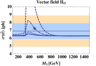
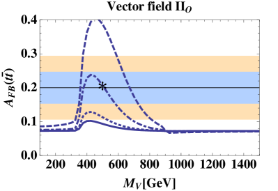
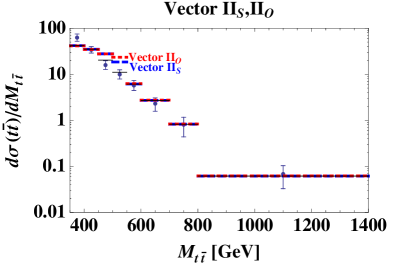
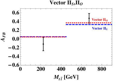
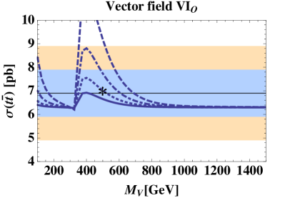
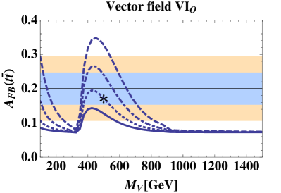
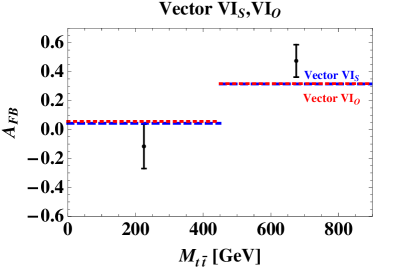
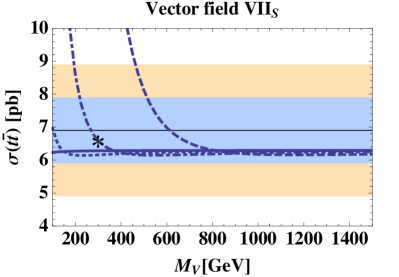
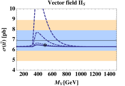
Figure 6: Upper two rows: predictions for total cross sections σ(tt¯)𝜎𝑡¯𝑡\sigma(t\bar{t}) and inclusive forward-backward asymmetry AFB(tt¯)subscript𝐴𝐹𝐵𝑡¯𝑡A_{FB}(t\bar{t}) as a function of vector mass mVsubscript𝑚𝑉m_{V} for models IIs,osubscriptIIso\rm II_{s,o} and couplings fqft=1/256subscript𝑓𝑞subscript𝑓𝑡1256f_{q}f_{t}=1/256 (solid curve), 1/12811281/128 (dotted), 1/321321/32 (dot-dashed), 1/8181/8 (dashed). The bands are the one and two σ𝜎\sigma measurements of AFBtt¯superscriptsubscript𝐴𝐹𝐵𝑡¯𝑡A_{FB}^{t\bar{t}} and σtt¯subscript𝜎𝑡¯𝑡\sigma_{t\,\bar{t}}. The predictions for AFBsubscript𝐴𝐹𝐵A_{FB} with Mtt¯subscript𝑀𝑡¯𝑡M_{t\bar{t}} below and above 450 GeV and for dσtt¯/dMtt¯𝑑subscript𝜎𝑡¯𝑡𝑑subscript𝑀𝑡¯𝑡d\sigma_{t\,\bar{t}}/dM_{t\,\bar{t}} are shown in the last row for benchmark points labeled with a \star in the inclusive predictions (MV=500subscript𝑀𝑉500M_{V}=500 GeV). The data are summarized in Table 3.
Refer to caption
Refer to caption
Refer to caption
Refer to caption
Refer to caption
Refer to caption
Figure 7: Same as Fig. 6 but for vector models VIs,osubscriptVIso\rm VI_{s,o} and couplings fqft=fqt2=1/42subscript𝑓𝑞subscript𝑓𝑡superscriptsubscript𝑓𝑞𝑡2142f_{q}f_{t}=f_{qt}^{2}=1/4\sqrt{2} (solid curve), 1/4141/4 (dotted), 1/2121/\sqrt{2} (dot-dashed), 22222\sqrt{2} (dashed) for model VssubscriptVs\rm V_{s} and couplings fqft=fqt2=1/16subscript𝑓𝑞subscript𝑓𝑡superscriptsubscript𝑓𝑞𝑡2116f_{q}f_{t}=f_{qt}^{2}=1/16 (solid curve), 1/8181/8 (dotted), 1/4141/4 (dot-dashed), 1/2121/2 (dashed) for model VosubscriptVo\rm V_{o}. For the benchmark points, mV=500subscript𝑚𝑉500m_{V}=500 GeV.
Refer to caption
Refer to caption
Refer to caption
Refer to caption
Refer to caption
Refer to caption
Figure 8: Same as Fig. 6 but for pure t𝑡t channel vector models VIIs,osubscriptVIIso\rm VII_{s,o} and coupling fqt=1/5subscript𝑓𝑞𝑡15f_{qt}=1/5 (solid curve), 4/5454/5 (dotted), 8/5858/5 (dot-dashed), 16/516516/5 (dashed) for model VssubscriptVs\rm V_{s} and couplings fqt=1/4subscript𝑓𝑞𝑡14f_{qt}=1/4 (solid curve), 111 (dotted), 9/4949/4 (dot-dashed), 444 (dashed) for model VosubscriptVo\rm V_{o}. For the benchmark points, mV=300subscript𝑚𝑉300m_{V}=300 GeV.
Refer to caption
Refer to caption
Refer to caption
Refer to caption
Refer to caption
Refer to caption
Refer to caption
Refer to caption
Figure 9: Predictions for dσ/dMtt¯𝑑𝜎𝑑subscript𝑀𝑡¯𝑡d\sigma/dM_{t\bar{t}} and AFBsubscript𝐴𝐹𝐵A_{FB} for a set of vector models, IVs,o,VIs,o,VIIIs,o,IXs,osubscriptIVsosubscriptVIsosubscriptVIIIso𝐼subscript𝑋𝑠𝑜{\rm IV_{s,o},VI_{s,o},VIII_{s,o}},IX_{s,o} fixing mV=subscript𝑚𝑉absentm_{V}=500 GeV (except for VIs,osubscriptVIso\rm VI_{s,o} where mV=subscript𝑚𝑉absentm_{V}=350 GeV, and using flavor breaking choices for couplings to quarks; (fqft,fqt)=(0.1,0.3)IVs;subscript𝑓𝑞subscript𝑓𝑡subscript𝑓𝑞𝑡0.10.3subscriptIVs(\sqrt{f_{q}f_{t}},f_{qt})=(0.1,0.3){\rm IV_{s}}; (0.1,0.3)IVo;(0.55,1.3)VIs;0.10.3subscriptIVo0.551.3subscriptVIs(0.1,0.3){\rm IV_{o}};(0.55,1.3){\rm VI_{s}}; (0.55,1.3)VIo0.551.3subscriptVIo(0.55,1.3){\rm VI_{o}} and (η1,η2)=(1.4,0.4)VIIIs;subscript𝜂1subscript𝜂21.40.4subscriptVIIIs(\eta_{1},\eta_{2})=(1.4,-0.4){\rm VIII_{s}}; (1.3,0.5)VIIIo;1.30.5subscriptVIIIo(1.3,-0.5){\rm VIII_{o}}; (1.1,0.4)IXs;1.10.4subscriptIXs(1.1,-0.4){\rm IX_{s}}; (1.1,0.4)IXo.1.10.4subscriptIXo(1.1,-0.4){\rm IX_{o}}.

III.1.3 The tt¯𝑡¯𝑡t\,\bar{t} phenomenology of HFsubscriptHF\rm H_{F} symmetric vector fields

In flavor symmetric scalar models, tt¯𝑡¯𝑡t\bar{t} production can only proceed via the u𝑢u or t𝑡t channels. Flavor symmetric vector models differ in this respect, as tt¯𝑡¯𝑡t\bar{t} production can also proceed in the s𝑠s channel or both in s𝑠s and t𝑡t channels simultaneously. Top phenomenology in these models is dictated to a large extent by which channel dominates. The sizes of the couplings required in order to explain the top asymmetry are roughly fixed by whether the vectors couple to up or down quarks in the initial states, as in the scalar models. The Lagrangians for the vector models are given in Section II and Appendix A. Expressions for the qq¯tt¯𝑞¯𝑞𝑡¯𝑡q\,\bar{q}\rightarrow t\,\bar{t} cross sections for models IXIIXI\rm I-XI are collected in Appendix B. They are given in terms of effective couplings of the vectors to light quarks (fqsubscript𝑓𝑞f_{q}), to top quarks (ftsubscript𝑓𝑡f_{t}), and to top and light quarks (fqtsubscript𝑓𝑞𝑡f_{qt}), defined in terms of η1,2subscript𝜂12\eta_{1,2} etc, see Table 7. In this section we use these couplings as numerical inputs. In the GFsubscriptGF\rm G_{F} symmetric limit (yt=0subscript𝑦𝑡0y_{t}=0), one has fq=ft=fqtsubscript𝑓𝑞subscript𝑓𝑡subscript𝑓𝑞𝑡f_{q}=f_{t}=f_{qt}. Among the vector models, IssubscriptIs\rm I_{s} and Vs,osubscriptVso\rm V_{s,o} do not contribute to top production, and IssubscriptIs\rm I_{s}, IIssubscriptIIs\rm II_{s} and IIIssubscriptIIIs\rm III_{s} do not interfere with the SM amplitude at tree-level.

We begin with an examination of the representative models IIs,osubscriptIIso\rm II_{s,o}, which only contribute in the s𝑠s-channel. The vector decay widths are given by mV(2fq2+ft2)/8πsubscript𝑚𝑉2superscriptsubscript𝑓𝑞2superscriptsubscript𝑓𝑡28𝜋m_{V}\,(2f_{q}^{2}+f_{t}^{2})/8\pi (IIssubscriptIIs\rm II_{s}) and mV(2fq2+ft2)/48πsubscript𝑚𝑉2superscriptsubscript𝑓𝑞2superscriptsubscript𝑓𝑡248𝜋m_{V}\,(2f_{q}^{2}+f_{t}^{2})/48\pi (IIosubscriptIIo\rm II_{o}), neglecting phase space suppression due to top quarks in the final state. In the first two rows of Fig. 6 we collect predictions for the inclusive AFBtt¯superscriptsubscript𝐴𝐹𝐵𝑡¯𝑡A_{FB}^{t\bar{t}} and σtt¯subscript𝜎𝑡¯𝑡{\sigma}_{t\,\bar{t}} as functions of the vector masses, for several values of the product fqftsubscript𝑓𝑞subscript𝑓𝑡f_{q}f_{t}. We have taken vector decay widths appropriate for the GFsubscriptGF\rm G_{F} symmetric limit: mV3fqft/8πsubscript𝑚𝑉3subscript𝑓𝑞subscript𝑓𝑡8𝜋m_{V}3f_{q}f_{t}/8\pi (IIssubscriptIIs\rm II_{s}) and mVfqft/16πsubscript𝑚𝑉subscript𝑓𝑞subscript𝑓𝑡16𝜋m_{V}f_{q}f_{t}/16\pi (IIosubscriptIIo\rm II_{o}). In the last row, predictions for dσ/dMtt¯𝑑𝜎𝑑subscript𝑀𝑡¯𝑡d\sigma/dM_{t\bar{t}} and AFBtt¯superscriptsubscript𝐴𝐹𝐵𝑡¯𝑡A_{FB}^{t\bar{t}} in the low and high Mtt¯subscript𝑀𝑡¯𝑡M_{t\bar{t}} bins are shown for the benchmark points (denoted by a \star). Good fits to the inclusive cross section and the top asymmetries can be obtained. However, agreement with dσ/dMtt¯𝑑𝜎𝑑subscript𝑀𝑡¯𝑡d\sigma/dM_{t\bar{t}} is much harder to achieve, as the effect of the s𝑠s-channel resonance is clear. The bounds from the Tevatron can be avoided if mV1TeVgreater-than-or-equivalent-tosubscript𝑚𝑉1TeVm_{V}\gtrsim 1\,{\rm TeV}. Unfortunately, for mV1TeVgreater-than-or-equivalent-tosubscript𝑚𝑉1TeVm_{V}\gtrsim 1\,{\rm TeV} and O(1)𝑂1O(1) couplings the effect on AFBtt¯superscriptsubscript𝐴𝐹𝐵𝑡¯𝑡A_{FB}^{t\bar{t}} is strongly reduced. The LHC dσ/dMtt¯𝑑𝜎𝑑subscript𝑀𝑡¯𝑡d\sigma/dM_{t\bar{t}} spectrum would also be problematic. It is possible, though, to hide a light s𝑠s channel resonance via an increase of its decay width due to additional non-qq¯𝑞¯𝑞q\bar{q} final states, as has recently been discussed in the context of pure s𝑠s-channel axial-vector models Tavares:2011zg . Another possibility for increasing the vector decay widths may be to consider the GFsubscriptGF\rm G_{F} breaking hierarchy fq2<<ft2much-less-thansuperscriptsubscript𝑓𝑞2superscriptsubscript𝑓𝑡2f_{q}^{2}<<f_{t}^{2}, keeping the product fqftsubscript𝑓𝑞subscript𝑓𝑡f_{q}f_{t} fixed.

The flavor octet models VIssubscriptVIs{\rm VI_{s}} and VIosubscriptVIo\rm VI_{o} contain admixtures of s𝑠s and t𝑡t channel contributions, while the flavor (3,3¯,1)3¯31(3,\bar{3},1) models VIIssubscriptVIIs{\rm VII_{s}} and VIIosubscriptVIIo{\rm VII_{o}} are purely t𝑡t channel. The s𝑠s channel contributions in VIs,osubscriptVIso{\rm VI_{s,o}} are due to the vectors associated with the generator T8superscript𝑇8T^{8} of SU(3)URSUsubscript3subscriptUR\rm SU(3)_{U_{R}} and the coupling product fqftsubscript𝑓𝑞subscript𝑓𝑡f_{q}f_{t}. The t𝑡t channel contributions are due to the vectors associated with the generators T4,..,7T^{4,..,7} and the coupling product fqt2superscriptsubscript𝑓𝑞𝑡2f_{qt}^{2}. While the generic problem of s𝑠s channel resonances persists, it is mitigated by their relative suppression compared to the t𝑡t channel contributions (the coefficients C1,2subscript𝐶12C_{1,2} are significantly smaller than C3subscript𝐶3C_{3} for these models, see Table 7), by possible cancelations between the two channels, and by the absence of interference between the SM and NP s𝑠s channel contribution in VIssubscriptVIs\rm VI_{s} (C5=0subscript𝐶50C_{5}=0). The s𝑠s channel effects can be further diminished, if the vector decay widths are enhanced by additional non-qq¯𝑞¯𝑞q\bar{q} final states.666Given that these models are by themselves non-renormalizable, it is reasonable to expect that renormalizable UV completions could contain additional vector decay modes. This assumption was implicit in the model VIosubscriptVIo\rm VI_{o} examples presented in Grinstein:2011yv and Fig. 1. In the following, we only consider vector decays to quark bilinears. In the GFsubscriptGF\rm G_{F} symmetric limit (fq=ft=fqtsubscript𝑓𝑞subscript𝑓𝑡subscript𝑓𝑞𝑡f_{q}=f_{t}=f_{qt}) the decay widths can be written as fqt2mV/16πsuperscriptsubscript𝑓𝑞𝑡2subscript𝑚𝑉16𝜋f_{qt}^{2}m_{V}/16\pi (VIssubscriptVIs\rm VI_{s} and VIIssubscriptVIIs\rm VII_{s}) and fqt2mV/96πsuperscriptsubscript𝑓𝑞𝑡2subscript𝑚𝑉96𝜋f_{qt}^{2}m_{V}/96\pi (VIosubscriptVIo\rm VI_{o} and VIIosubscriptVIIo\rm VII_{o}). Finally, s𝑠s channel effects in VIs,osubscriptVIso\rm VI_{s,o} would be suppressed in the GFsubscriptGF\rm G_{F} breaking limit fqft<<fqt2much-less-thansubscript𝑓𝑞subscript𝑓𝑡superscriptsubscript𝑓𝑞𝑡2f_{q}f_{t}<<f_{qt}^{2} (this breaking is natural due to the large top yukawa), and would be absent entirely in the minimal HFsubscriptHF\rm H_{F} symmetric realizations which only contain the complex SU(2)URSUsubscript2subscriptUR\rm SU(2)_{U_{R}} doublets associated with the SU(3)UR𝑆𝑈subscript3subscript𝑈𝑅SU(3)_{U_{R}} flavor generators T4,..,7T^{4,..,7}.

We show the effect of the models VIs,osubscriptVIso{\rm VI_{s,o}} and VIIs,osubscriptVIIso\rm VII_{s,o} on AFBtt¯superscriptsubscript𝐴𝐹𝐵𝑡¯𝑡A_{FB}^{t\,\bar{t}} and σtt¯subscript𝜎𝑡¯𝑡\sigma_{t\,\bar{t}} in the GFsubscriptGF\rm G_{F} symmetric limit in Figs. 7 and  8, respectively. In the purely t𝑡t-channel models VIIs,osubscriptVIIso\rm VII_{s,o}, we see that it is possible to enhance AFBtt¯superscriptsubscript𝐴𝐹𝐵𝑡¯𝑡A_{FB}^{t\,\bar{t}}, while at the same time not introducing any visible deviations in the dσ/dmtt¯𝑑𝜎𝑑subscript𝑚𝑡¯𝑡d\sigma/dm_{t\bar{t}} differential spectrum. For models VIs,osubscriptVIso{\rm VI_{s,o}}, on the other hand, we see that it is difficult to enhance AFBtt¯superscriptsubscript𝐴𝐹𝐵𝑡¯𝑡A_{FB}^{t\,\bar{t}} sufficiently, without obtaining excessive s𝑠s channel peaks in the dσ/dMtt¯𝑑𝜎𝑑subscript𝑀𝑡¯𝑡d\sigma/dM_{t\bar{t}} spectra, as in the model IIs,osubscriptIIso\rm II_{s,o} examples above. However, as already noted, much better agreement with the measured spectrum can be achieved in this case, if GFsubscriptGF{\rm G_{F}} is broken down to its subgroup HFsubscriptHF{\rm H_{F}}777Whereas in models VIIs,osubscriptVIIso\rm VII_{s,o} the GFHFsubscriptGFsubscriptHF\rm G_{F}\to H_{F} breaking is not needed in order to obtain good agreement with the dσ/dmtt¯𝑑𝜎𝑑subscript𝑚𝑡¯𝑡d\sigma/dm_{t\bar{t}} spectrum, it may be required to evade dijet and BKπ𝐵𝐾𝜋B\to K\pi constraints.. In Fig. 9 we show such examples, with fqft<<fqt2much-less-thansubscript𝑓𝑞subscript𝑓𝑡superscriptsubscript𝑓𝑞𝑡2f_{q}f_{t}<<f_{qt}^{2}, for various vector models. The decay widths of the different vectors in a GFsubscriptGF\rm G_{F} multiplet will not be equal in this limit. For simplicity, we have identified all the widths in each multiplet with the quantities mVfqft/16π×m_{V}f_{q}f_{t}/16\pi\times (3,1/2,1,1/6,2,1/3,1/2,1/12)31211621312112(3,1/2,1,1/6,2,1/3,1/2,1/12) in models IVssubscriptIVs\rm IV_{s}, IVosubscriptIVo\rm IV_{o}, VIssubscriptVIs\rm VI_{s}, VIosubscriptVIo\rm VI_{o}, VIIIssubscriptVIIIs\rm VIII_{s}, VIIIosubscriptVIIIo\rm VIII_{o}, IXssubscriptIXs\rm IX_{s}, IXosubscriptIXo\rm IX_{o}, respectively (which would hold in the GFsubscriptGF\rm G_{F} symmetric limit, neglecting phase space differences). The rationale for this approximation is that the s𝑠s channel resonance widths are associated with the coupling products fq2superscriptsubscript𝑓𝑞2f_{q}^{2} and ft2subscriptsuperscript𝑓2𝑡f^{2}_{t}, whereas the widths of the t𝑡t channel resonances, controlled by the product fqt2superscriptsubscript𝑓𝑞𝑡2f_{qt}^{2}, have minimal impact on the Mtt¯subscript𝑀𝑡¯𝑡M_{t\bar{t}} spectrum. In addition, as we will see in Section IV.3 (see Table 6), dijet constraints on the light quark vector couplings fqsubscript𝑓𝑞f_{q} are relatively mild, so that the relation fq2=ft2=fqftsubscriptsuperscript𝑓2𝑞subscriptsuperscript𝑓2𝑡subscript𝑓𝑞subscript𝑓𝑡f^{2}_{q}=f^{2}_{t}=f_{q}f_{t} would be phenomenologically viable in the light vector examples of Fig. 9.

III.1.4 Limits from LHC measurements of the tt¯𝑡¯𝑡t\,\bar{t} invariant mass spectrum.

Recently, the first measurements of the tt¯𝑡¯𝑡t\bar{t} invariant mass spectrum at the LHC have been presented by the ATLAS and CMS collaborations. With up to 0.70.70.7 pb-1 the ATLAS collaboration obtains σtt¯=176±5(stat)10+13(syst.)±7(lumi.)\sigma_{t\bar{t}}=\rm 176\pm 5(stat)^{+13}_{-10}(syst.)\pm 7(lumi.) pb, while using 36pb136psuperscriptb136{\rm pb}^{-1} the CMS collaboration obtains a combined cross section σtt¯=158±10(uncor.)±15(cor.)±6(lumi.)\sigma_{t\bar{t}}=\rm 158\pm 10(uncor.)\pm 15(cor.)\pm 6(lumi.) pb cmsnote . This is to be compared with the NLO+NNLL predictions or the approximate NNLO predictions for the inclusive cross section that are listed in Ref. Ahrens:2011mw , and range between σtt¯=157±13subscript𝜎𝑡¯𝑡plus-or-minus15713\sigma_{t\bar{t}}=157\pm 13 pb and σtt¯=145±11subscript𝜎𝑡¯𝑡plus-or-minus14511\sigma_{t\bar{t}}=145\pm 11 pb, depending on the approximation used. ATLAS and CMS have also presented promising first measurements of the differential cross section at 200 pb-1 and 886 pb-1 CMS-Mulders-talk , respectively.
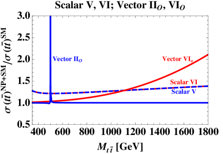
Refer to caption
Figure 10: Predictions for the ratio (dσ(tt¯)NP+SM/dMtt¯)/(dσ(tt¯)SM/dMtt¯)𝑑𝜎subscript𝑡¯𝑡𝑁𝑃𝑆𝑀𝑑subscript𝑀𝑡¯𝑡𝑑𝜎subscript𝑡¯𝑡𝑆𝑀𝑑subscript𝑀𝑡¯𝑡(d\sigma(t\,\bar{t})_{NP+SM}/dM_{t\bar{t}})/(d\sigma(t\,\bar{t})_{SM}/dM_{t\bar{t}}) for scalar and vector models. The scalar model examples are for model SVsubscriptSV\rm S_{V} with (η,mS)=𝜂subscript𝑚𝑆absent(\eta,m_{S})= (1,400GeV)1400GeV(1,400\,{\rm GeV}) dashed blue, and for model SVIsubscriptSVI\rm S_{VI} with (η,mS)=𝜂subscript𝑚𝑆absent(\eta,m_{S})= (1/2,800GeV)12800GeV(1/\sqrt{2},800\,{\rm GeV}) dotted red. The vector model examples are for IIosubscriptIIo\rm II_{o} with (fq=ft,MV)=subscript𝑓𝑞subscript𝑓𝑡subscript𝑀𝑉absent(f_{q}=f_{t},M_{V})= (1/32,500GeV)132500GeV(1/\sqrt{32},500\,{\rm GeV}) solid blue, and for with (fqft,fqt,MV)=subscript𝑓𝑞subscript𝑓𝑡subscript𝑓𝑞𝑡subscript𝑀𝑉absent(f_{q}\,f_{t},f_{qt},M_{V})= (0.5,2,500GeV)0.52500GeV(0.5,2,500\,{\rm GeV}) solid red.

In the near future the differential cross section measurements will place meaningful constraints on the models we have considered. We therefore present below some representative examples of their impact on the differential spectrum. In Fig. 10 we show the ratio

Rσ=dσ(tt¯)NP+SM/dMtt¯dσ(tt¯)SM/dMtt¯.subscript𝑅𝜎𝑑𝜎subscript𝑡¯𝑡𝑁𝑃𝑆𝑀𝑑subscript𝑀𝑡¯𝑡𝑑𝜎subscript𝑡¯𝑡𝑆𝑀𝑑subscript𝑀𝑡¯𝑡R_{\sigma}=\frac{d\sigma(t\,\bar{t})_{NP+SM}/dM_{t\bar{t}}}{d\sigma(t\,\bar{t})_{SM}/dM_{t\bar{t}}}. (24)

in models IIo,VIo,SV,subscriptIIosubscriptVIosubscriptSV\rm II_{o},VI_{o},S_{V}, and SVIsubscriptSVI\rm S_{VI} for the benchmark points shown in Figs. 6, 7, and 9. In the ratio we use SM NLO+NNLL prediction from Ref. Ahrens:2010zv , while NP contribution including interference with the SM is calculated at LO, mirroring our procedure for Tevatron predictions used in previous sections. In Fig. 10 a sharp resonant peak is clearly visible for the disfavored pure s𝑠s-channel model IIosubscriptIIo\rm II_{o}. Once convoluted with the experimental resolution the peak will be less prominent. For instance assuming 10 GeV resolution the peak leads to an 𝒪(30%)𝒪percent30{\mathcal{O}}(30\%) enhancement of the cross section in the bin containing the peak. The model VIosubscriptVIo\rm VI_{o} example contains a rise in the tail region associated with the Rutherford scattering peak that is characteristic of t𝑡t-channel models with 𝒪(1)𝒪1{\mathcal{O}}(1) couplings. The scalar models SVsubscriptSV\rm S_{V} and SVIsubscriptSVI\rm S_{VI}, being u𝑢u-channel models, display a relative enhancement throughout the entire differential spectrum Gresham:2011fx , similarly to the case at Tevatron (see Fig. 3). Model SIsubscriptSI\rm S_{I} displays virtually no deviation from the SM spectrum, as pointed out in Refs. AguilarSaavedra:2011ug ; Blum:2011fa .

III.2 Contributions to BsB¯ssubscript𝐵𝑠subscript¯𝐵𝑠B_{s}-\bar{B}_{s} mixing

There is some evidence for NP contributions to the measurement of the Bssubscript𝐵𝑠B_{s} mixing phase. A 3.9σ𝜎\sigma deviation from the negligible SM prediction has been measured in the like-sign dimuon charge asymmetry by the DØ collaboration Williams:2011nc ; Abazov:2010hv . This result is in agreement Ligeti:2010ia ; Lenz:2010gu with a hint for a nonzero weak phase in Bssubscript𝐵𝑠B_{s} mixing (measured through flavor tagged decays D0-6098-CONF ; CDF-10206 ). The hints for NP in Bssubscript𝐵𝑠B_{s} mixing have two preferred solutions Ligeti:2010ia , with

hs0.5,σs130andhs2,σs100.formulae-sequenceformulae-sequencesimilar-tosubscript𝑠0.5similar-tosubscript𝜎𝑠superscript130andsubscript𝑠similar-to2similar-tosubscript𝜎𝑠superscript100h_{s}\sim 0.5,\sigma_{s}\sim 130^{\circ}{\rm~{}and~{}}h_{s}\sim 2,\sigma_{s}\sim 100^{\circ}. (25)

Here, hs,dsubscript𝑠𝑑h_{s,d} and 2σs,d2subscript𝜎𝑠𝑑2\sigma_{s,d} denote the magnitude and phase, respectively, of the NP contribution to the Bs,dsubscript𝐵𝑠𝑑B_{s,d} mixing amplitude, normalized to the SM one (see also (97)). Note that the above results have been obtained using the older measurement of the dimuon asymmetry Abazov:2010hv . Since the two measurements are consistent, we do not expect a significant change in the position of the two minima. There is also a slight preference for hd0.2similar-tosubscript𝑑0.2h_{d}\sim 0.2, σd100similar-tosubscript𝜎𝑑superscript100\sigma_{d}\sim 100^{\circ}, but at slightly more than 1σ1𝜎1\sigma hdsubscript𝑑h_{d} is consistent with zero. At 3σ3𝜎3\sigma one finds hd<0.5subscript𝑑0.5h_{d}<0.5 for all σdsubscript𝜎𝑑\sigma_{d} Ligeti:2010ia .

The flavor symmetric models can be grouped by whether or not they can give contributions to BsB¯ssubscript𝐵𝑠subscript¯𝐵𝑠B_{s}-\bar{B}_{s} mixing. The models in which the new fields only couple to uRsubscript𝑢𝑅u_{R} fall into the latter category These are models IIs,osubscriptII𝑠𝑜{\rm II}_{s,o}, VIs,osubscriptVIso{\rm VI_{s,o}} and SV,VIsubscriptSVVI{\rm S_{V,VI}}. Then there are models in which the NP contributions first arise at loop level: VIIs,osubscriptVIIso{\rm VII_{s,o}} and SIX,XsubscriptSIXX{\rm S_{IX,X}}, which couple to dRsubscript𝑑𝑅d_{R} and uRsubscript𝑢𝑅u_{R}, ,XI3¯,6{\rm,XI_{\bar{3},6}} and SI,IIsubscriptSIII{\rm S_{I,II}} that couple to uRsubscript𝑢𝑅u_{R} and QLsubscript𝑄𝐿Q_{L}. For the remaining models tree level contributions to Bssubscript𝐵𝑠B_{s} mixing are possible.

For a quantitative analysis one needs to specify the HFsubscriptHF{\rm H_{F}} breaking. We will adopt the MFV hypothesis, assuming that the breaking in the NP sector is only due to the SM Yukawa couplings. (for an example with maximal breaking of HFsubscript𝐻𝐹H_{F} see Shelton:2011hq ). This hypothesis ensures that the FCNCs generated from the exchange of NP fields have SM CKM suppression, making the FCNC constraints easier to satisfy. MFV scalar fields that can lead to the dimuon anomaly have been discussed in the literature previously Blum:2010mj ; Buras:2010pz ; Buras:2010zm ; Trott:2010iz . We begin by classifying the flavor symmetric vector and scalar fields that can contribute to Bssubscript𝐵𝑠B_{s} mixing at tree level. Most of the details are relegated to Appendix C.

The MFV models fall in two categories:“universal models” leading to class 1 ΔB=2Δ𝐵2\Delta B=2 mixing operators in the terminology of Kagan:2009bn , and “yukawa suppressed” models that give rise to class 2 operators and are additionally suppressed by light quark yukawa couplings, ys,dsubscript𝑦𝑠𝑑y_{s,d}. In universal models the NP contributions (normalized to the SM) are equal in the Bssubscript𝐵𝑠B_{s} and Bdsubscript𝐵𝑑B_{d} mixing amplitudes. This is in some tension with experiment, where there are indications for large effects in Bssubscript𝐵𝑠B_{s} mixing, i.e., 50%200%percent50percent20050\%-200\% of the SM amplitude. Measurements in the Bdsubscript𝐵𝑑B_{d} system, on the other hand, can accommodate a NP contribution of up to 20%similar-toabsentpercent20\sim 20\%. Universal models can thus explain the dimuon anomaly only if the real effect is on the lower end of the experimentally preferred range for Bssubscript𝐵𝑠B_{s} mixing and on the upper range for Bdsubscript𝐵𝑑B_{d} mixing.

The simplest examples of universal MFV models that can explain the dimuon anomaly are the two scalar doublet model, where in our notation the higgs linear combination without a vev is SHsubscriptSH{\rm S_{H}} Buras:2010pz ; Buras:2010zm ; Trott:2010iz , and the color-octet, weak-doublet scalar model S8subscriptS8{\rm S_{8}} Manohar:2006ga . Effects are large even for mS=1subscript𝑚𝑆1m_{S}=1 TeV, if the couplings of the flavor breaking terms ηisubscript𝜂𝑖\eta_{i} and the bottom Yukawa coupling ybsubscript𝑦𝑏y_{b} are 𝒪(1)𝒪1{\mathcal{O}}(1). For the SM value yb0.02similar-tosubscript𝑦𝑏0.02y_{b}\sim 0.02 the mass scale for the new uncharged scalars would have to be quite low. Such a low mass scale, surprisingly, is consistent with present phenomenology for S8subscriptS8{\rm S_{8}} Burgess:2009wm . Similar comments apply to the other universal models, IIIs,o,IVs,o,VIIIs,o,IXs,osubscriptIIIsosubscriptIVsosubscriptVIIIsosubscriptIXso{\rm III_{s,o},IV_{s,o},VIII_{s,o},IX_{s,o}} and SXIVsubscriptSXIV\rm S_{XIV}. In order to obtain the right size of hssubscript𝑠h_{s} for the dimuon anomaly one needs ηi0.1similar-tosubscript𝜂𝑖0.1\eta_{i}\sim 0.1, if mS,V=1subscript𝑚𝑆𝑉1m_{S,V}=1 TeV.

The yukawa suppressed models can have mixing amplitudes suppressed either by one power or two powers of light yukawas. For ys2superscriptsubscript𝑦𝑠2y_{s}^{2} suppressed models, Is,o,Vs,osubscriptIsosubscriptVso{\rm I_{s,o},V_{s,o}} and SVIIIsubscriptSVIII\rm S_{VIII}, the Bssubscript𝐵𝑠B_{s} mixing anomaly can be potentially explained only if yb,ηi𝒪(1)similar-tosubscript𝑦𝑏subscript𝜂𝑖𝒪1y_{b},\eta_{i}\sim{\mathcal{O}}(1) and the masses of NP fields are no more that a few 100 GeV. The NP contributions to Bdsubscript𝐵𝑑B_{d} are predicted to be too small to be observed in this case, since they are additionally suppressed by yd2/ys2superscriptsubscript𝑦𝑑2superscriptsubscript𝑦𝑠2y_{d}^{2}/y_{s}^{2}. The singly yssubscript𝑦𝑠y_{s} suppressed models, X3¯,6subscriptX¯36{\rm X_{\bar{3},6}} and SI,SIIIsubscriptSIsubscriptSIII{\rm S_{I},S_{III}}, give contributions to hssubscript𝑠h_{s} of the right order of magnitude for ηi𝒪(1)similar-tosubscript𝜂𝑖𝒪1\eta_{i}\sim{\mathcal{O}}(1) and mS,V1similar-tosubscript𝑚𝑆𝑉1m_{S,V}\sim 1 TeV. There is also an effect predicted for Bdsubscript𝐵𝑑B_{d} mixing with size hd0.1similar-tosubscript𝑑0.1h_{d}\sim 0.1.

A number of flavor symmetric models can potentially explain both the Bssubscript𝐵𝑠B_{s} mixing and AFBtt¯superscriptsubscript𝐴𝐹𝐵𝑡¯𝑡A_{FB}^{t\bar{t}} anomalies simultaneously. If enhanced Bssubscript𝐵𝑠B_{s} mixing is due to tree level exchange, the NP fields need to couple to left-handed doublets if they are to also contribute to tt¯𝑡¯𝑡t\bar{t} production. The relevant models are IIIs,o,IVs,o,VIIIs,osubscriptIIIsosubscriptIVsosubscriptVIIIso{\rm III_{s,o},IV_{s,o},VIII_{s,o}} and IXs,osubscriptIX𝑠𝑜{\rm IX}_{s,o}, where for TeV masses, the flavor breaking couplings need to be ηi𝒪(0.1)similar-tosubscript𝜂𝑖𝒪0.1\eta_{i}\sim{\mathcal{O}}(0.1). However, none of these models seem to fit the observed data in top pair production particularly well (See Fig. 9 for models IVs,o,VIIIs,osubscriptIVsosubscriptVIIIso\rm IV_{s,o},VIII_{s,o} and IXs,osubscriptIX𝑠𝑜{\rm IX}_{s,o}. The models IIIs,osubscriptIIIso{\rm III_{s,o}} are pure s𝑠s-channel and thus lead to large deviations in the tt¯𝑡¯𝑡t\bar{t} differential cross section.).

There are also four models of interest that exhibit linear Yukawa suppression and can in principle contribute to Bssubscript𝐵𝑠B_{s} mixing and to the AFBtt¯superscriptsubscript𝐴𝐹𝐵𝑡¯𝑡A_{FB}^{t\bar{t}} anomaly simultaneously. These are models X3¯,6subscriptX¯36{\rm X}_{\bar{3},6} and models SIIIsubscriptSIII{\rm S_{III}}, SIVsubscriptSIV{\rm S_{IV}}. However, due to their color representation SIIIsubscriptSIII\rm S_{III}, SIVsubscriptSIV\rm S_{IV}, have limited potential to explain AFBtt¯superscriptsubscript𝐴𝐹𝐵𝑡¯𝑡A_{FB}^{t\bar{t}}, while X3¯,6subscriptX¯36{\rm X}_{\bar{3},6} reduce rather than increase AFBtt¯superscriptsubscript𝐴𝐹𝐵𝑡¯𝑡A_{FB}^{t\bar{t}}.

This leaves us with models where the contributions to Bssubscript𝐵𝑠B_{s} mixing are loop suppressed. These are the vector models VIIs,osubscriptVIIso{\rm VII_{s,o}}, XI3¯,6subscriptXI¯36{\rm XI_{\bar{3},6}} and the scalar models SI,SIIsubscriptSIsubscriptSII{\rm S_{I},S_{II}}, SIX,XsubscriptSIXX{\rm S_{IX,X}}. They lead to contributions to Bssubscript𝐵𝑠B_{s} and Bdsubscript𝐵𝑑B_{d} mixing which are universal, if one assumes MFV. Among these, models VIIs,osubscriptVIIso{\rm VII_{s,o}} and SIsubscriptSI{\rm S_{I}} can also explain the present top data. The contributions to Bssubscript𝐵𝑠B_{s} mixing can also carry a new weak phase, as required by the dimouon charge asymmetry.

For instance, model SIsubscriptSI{\rm S_{I}}, see Eq. (21), contains contributions that are proportional to the product of the generally complex quantity 4η02η324superscriptsubscript𝜂02superscriptsubscript𝜂324\eta_{0}^{2}\eta_{3}^{2} (where these coefficients are defined in Table 10 in Appendix C) with a loop function that is of the same order of magnitude as the SM one, with its precise value depending on the size of mSsubscript𝑚𝑆m_{S}. The BKπ𝐵𝐾𝜋B\to K\pi branching ratios require η0η3<1/4subscript𝜂0subscript𝜂3<14\sqrt{\eta_{0}\eta_{3}}{~{}\raise 1.49994pt\hbox{$<$}\kern-8.50006pt\lower 3.50006pt\hbox{$\sim$}~{}}1/4 (see Section IV.4), while AFBtt¯superscriptsubscript𝐴𝐹𝐵𝑡¯𝑡A_{FB}^{t\bar{t}} favors η01similar-tosubscript𝜂01\eta_{0}\sim 1. Thus, CPV contributions to Bssubscript𝐵𝑠B_{s} mixing of 𝒪(20%)𝒪percent20{\mathcal{O}}(20\%) are readily attainable for SIsubscriptSI\rm S_{I} scalar masses of order 100 GeV. Similar considerations apply to models VIIs,osubscriptVIIso\rm VII_{s,o}.

IV Existing experimental constraints on a flavor symmetric sector

We now determine some of the existing experimental constraints on flavor symmetric extensions of the SM. We examine bounds on direct production at LEP, from electroweak precision data (EWPD) and from collider searches at the Tevatron and LHC. We also determine the (residual) FCNC constraints.

Our aim is characterize the general phenomenological bounds whenever possible and to check if some of the models that we have identified as promising candidates are consistent with other phenomenology in some detail. Our results are not completely comprehensive, as at times we have to focus on particular sample models. However, we believe our results are valuable to gain some intuition as to the current phenomenological constraints on a flavor symmetric sector.

IV.1 LEP Constraints

The LEP constraints depend on how the new states couple to electrons and to the pair of final state fermions. In this section we will discuss the constraints on the vector models from LEP in some detail. The constraints for scalar models are very similar, see Arnold:2009ay for some details. Limits on anomalous four jet events at LEP give a kinematic lower bound for pair production of the scalar models of 105GeV105GeV105\,{\rm GeV} Arnold:2009ay . For the vector and scalar models signals that involve couplings to quarks and leptons are the most problematic at LEP. For a Zsuperscript𝑍Z^{\prime} vector boson that couples to quarks (electrons) with couplings gzzfBsubscript𝑔𝑧subscript𝑧𝑓𝐵g_{z}z_{fB} (gzzeAsubscript𝑔𝑧subscript𝑧𝑒𝐴g_{z}z_{eA}), the bound is Carena:2004xs

MZ2gz24π|zeAzfB|(ΛABf)2.superscriptsubscript𝑀superscript𝑍2superscriptsubscript𝑔𝑧24𝜋subscript𝑧𝑒𝐴subscript𝑧𝑓𝐵superscriptsuperscriptsubscriptΛ𝐴𝐵𝑓2\displaystyle M_{Z^{\prime}}^{2}\geq\,\frac{g_{z}^{2}}{4\,\pi}\,|z_{eA}\,z_{fB}|\,(\Lambda_{AB}^{f})^{2}\,. (26)

with A,B={L,R}𝐴𝐵𝐿𝑅A,B=\{L,R\} the chirality of the fermions. Typically ΛABf10TeVsimilar-tosuperscriptsubscriptΛ𝐴𝐵𝑓10TeV\Lambda_{AB}^{f}\sim 10~{}\rm TeV, leading to mass bounds on the order of MZ1TeVgreater-than-or-equivalent-tosubscript𝑀superscript𝑍1TeVM_{Z^{\prime}}\gtrsim 1~{}{\rm TeV}.

The vectors in nontrivial color or flavor representations (IoIVosubscriptIosubscriptIVo{\rm I_{o}-IV_{o}} or VXIVXI{\rm V-XI}) are protected from having tree level exchanges of this form. For models protected by flavor symmetry one is forced to have the insertion of Yukawa matrices. The final operating energy of LEP was s=209<2mt𝑠2092subscript𝑚𝑡\sqrt{s}=209<2m_{t} so the flavor symmetry is sufficient to remove this bound for models VXIVXI\rm V-XI. These bounds do apply to IsIVssubscriptIssubscriptIVs\rm I_{s}-IV_{s} unless the couplings to electrons are somehow suppressed, e.g., by extending flavor symmetry to the lepton sector.

Refer to caption

Figure 11: Tree level generation of multi-jet events at LEP due to flavor symmetric vectors. Similar diagrams (and bounds) exist for scalars and the first diagram is representative of the emissions of the vectors and scalars off the final state fermions.

For the models where the bound (26) does not hold, there are constraints from covariant derivative couplings to Z𝑍Z and γ𝛾\gamma in the kinetic terms of the vectors (the factor N𝑁N is set by requiring canonical normalization),

K=NTr(DμVνDμVνDμVνDνVμ).subscript𝐾𝑁Trsubscript𝐷𝜇subscriptsuperscript𝑉𝜈superscript𝐷𝜇superscript𝑉𝜈subscript𝐷𝜇subscriptsuperscript𝑉𝜈superscript𝐷𝜈superscript𝑉𝜇\displaystyle\mathcal{L}_{K}=N\text{Tr}\left(D_{\mu}V^{\dagger}_{\nu}\,D^{\mu}V^{\nu}-D_{\mu}V^{\dagger}_{\nu}\,D^{\nu}V^{\mu}\right)\,. (27)

Some tree level processes that would lead to anomalous four jet events at LEP are shown in Fig. 11. These processes do proceed even in the absence of flavor violation. Furthermore, for vector pair production (the second diagram) the couplings of the Z𝑍Z or γ𝛾\gamma to the vectors are fixed by gauge invariance. This implies a kinematic bound of MV105GeVgreater-than-or-equivalent-tosubscript𝑀𝑉105GeVM_{V}\gtrsim 105~{}{\rm GeV} on the flavor symmetric vectors. The analogous diagram for the scalar models is the origin of the kinematic bound on the scalar masses discussed in Arnold:2009ay .

The first diagram(s) can lead to a stronger bound for a vector or a scalar model as the vector or scalar is singly produced and has an order one branching ratio to anomalous multi-jet final states due to the flavor quantum numbers it carries. We find that this production process gives a cross section of 0.20|η|2pb10.20superscript𝜂2superscriptpb10.20|\eta|^{2}~{}\text{pb}^{-1} for MV=120GeVsubscript𝑀𝑉120GeVM_{V}=120\,{\rm GeV}, or, with an integrated luminosity of 500500500 pb above this mass scale, a total of 100|η|2100superscript𝜂2100|\eta|^{2} events. The number of expected events falls rapidly with increasing MVsubscript𝑀𝑉M_{V} and is below 12|η|212superscript𝜂212|\eta|^{2} for MV140GeVsubscript𝑀𝑉140GeVM_{V}\geq 140\,{\rm GeV}. Assuming an order one branching ratio to anomalous multi-jet final states, this implies that the mass bound on the vectors from LEP is MV150GeVgreater-than-or-equivalent-tosubscript𝑀𝑉150GeVM_{V}\gtrsim 150\,{\rm GeV} for 𝒪(1)𝒪1{\mathcal{O}}(1) couplings. Colored vectors will have similar mass bounds from LEP from anomalous multijet events. The calculation for the scalar models is very similar, resulting in the same approximate bounds.

In summary, we consider the minimum LEP lower bound for all vector and scalar models to be 150GeVgreater-than-or-equivalent-toabsent150GeV\gtrsim 150\,{\rm GeV} when order one couplings exist for the fields to quarks. A dedicated study would be required for each model to obtain more precise bounds. However, we note that while scalar (doublet) masses below 150 GeV were only considered in model SIsubscriptSI\rm S_{I}, see Eq. 22, for enhancing AFBtt¯superscriptsubscript𝐴𝐹𝐵𝑡¯𝑡A_{FB}^{t\bar{t}}, this bound could easily be evaded by making the charged components of the scalar doublets heavier. Single exchange of the neutral components (the ones involved in tt¯𝑡¯𝑡t\bar{t} production), as in the scalar analog of the first diagram of Fig. 11, would lead to kinematically suppressed virtual tt¯𝑡¯𝑡t\bar{t} pair production. The LEP bound can be generically stronger for a color singlet that does not transform under the flavor group: for vectors IsIVssubscriptIssubscriptIVs\rm I_{s}-IV_{s} the lower mass bound is 1TeVgreater-than-or-equivalent-toabsent1TeV\gtrsim 1\,{\rm TeV} for order one couplings to leptons and quarks.

IV.2 Electroweak precision tests

We consider the models for massive HFsubscriptHF\rm H_{F} symmetric vector and scalar fields to be effective field theories. Up to this point we have assumed that the cut-off of the theory, ΛΛ\Lambda, is high enough that we can neglect operators suppressed by powers of ΛΛ\Lambda. For the scalar models, in principle, we do not have to consider effects of higher dimensional operators. In this case, for scalar models that are SUL(2)subscriptSUL2\rm SU_{L}(2) singlets, the results of Arnold:2009ay show that the generic lower bound from fitting to EWPD is ms100GeVgreater-than-or-equivalent-tosubscript𝑚𝑠100GeVm_{s}\gtrsim 100~{}{\rm GeV}. The LEP bounds we have just derived are stronger than these bounds for scalar models that do not break custodial symmetry.

Below, we summarize our findings for model SIsubscriptSI\rm S_{I}, for which particularly light scalar doublets were considered in the context of AFBt¯tsuperscriptsubscriptAFB¯tt\rm A_{FB}^{\bar{t}t}. We find that it is easily consistent with S𝑆S parameter bounds, even in the presence of nine light doublets, as in the GFsubscriptGF\rm G_{F} symmetric realization, rather than only two, as in the minimal HFsubscriptHF\rm H_{F} symmetric versions I(a) - I(c) (Eqs. (21) – (23)) considered in the previous section (we have generalized the analysis of Blum:2011fa for a single scalar doublet). The T𝑇T parameter bounds are easily satisfied in the minimal versions, with neutral scalar doublet component masses as low as 110 GeV and heavier charged component masses of 150 GeV, a mass splitting that may be required in order to simultaneously evade the LEP bounds discussed above and enhance AFBtt¯superscriptsubscript𝐴𝐹𝐵𝑡¯𝑡A_{FB}^{t\bar{t}} to observed levels. Mass splitting between the charged and neutral scalar doublet components can be obtained via GFsubscriptGF\rm G_{F} symmetric couplings to the SM Higgs vacuum expectation value. We have also checked the sizes of non-oblique corrections in the minimal versions of SIsubscriptSI\rm S_{I}. In options I(a) and I(c), loop graphs containing the top quark lead to problematic shifts in the LH down and strange quark couplings to the Z𝑍Z. For instance, taking charged scalar masses of 150 GeV, neutral scalar masses of 110 GeV, and couplings η2/3𝜂23\eta\approx 2/3 yields δgsL/gsL,δgdL/gdL0.0046𝛿subscript𝑔subscript𝑠𝐿subscript𝑔subscript𝑠𝐿𝛿subscript𝑔subscript𝑑𝐿subscript𝑔subscript𝑑𝐿0.0046\delta g_{s_{L}}/g_{s_{L}},\,\delta g_{d_{L}}/g_{d_{L}}\approx-0.0046, roughly 2σ2𝜎2\sigma in excess of the 2 σ𝜎\sigma upper bound obtained, for equal shifts in the two couplings, from the Z𝑍Z hadronic width. In option I(b), loop graphs containing the charm and up quarks lead to a shift in the LH bottom quark coupling to the Z𝑍Z. For the same parameter choices (see Fig. 5) the shift is δgbL/gbL0.0028𝛿subscript𝑔subscript𝑏𝐿subscript𝑔subscript𝑏𝐿0.0028\delta g_{b_{L}}/g_{b_{L}}\approx-0.0028, which is consistent with Rbsubscript𝑅𝑏R_{b} at 2σ2𝜎2\sigma. We therefore conclude that whereas I(b) is a viable option for enhancing AFBtt¯superscriptsubscript𝐴𝐹𝐵𝑡¯𝑡A_{FB}^{t\bar{t}}, this is unlikely for cases I(a) and I(c).

For the massive vector fields we do have to consider the effects of higher dimensional operators suppressed by the cut off scale as the theory is nonrenormalizable. This is particularly the case when considering electroweak precision data (EWPD) for vectors. To the effective fields we have considered at the scale μMVsimilar-to𝜇subscript𝑀𝑉\mu\sim M_{V} we should add dimension six operators. These arise from integrating out heavier modes of the UV complete theory. At the electroweak scale μmZsimilar-to𝜇subscript𝑚𝑍\mu\sim m_{Z} we integrate out also the vectors and can match onto an effective field theory constructed from only the SM fields, appropriate for examining EWPD. The dimension six operators then receive contributions from vectors and from heavier fields from the UV completion.

For cases IsIVssubscriptIssubscriptIVs\rm I_{s}-IV_{s}, the EFT will in general have a dangerous dimension 4 operator 𝒪1=Vμ(HDμH)subscript𝒪1superscript𝑉𝜇superscript𝐻subscript𝐷𝜇𝐻\mathcal{O}_{1}=V^{\mu}\,(H^{\dagger}\,D_{\mu}\,H). Integrating out the vectors gives the dimension six operator 𝒪T=|HDμH|2/MV2subscript𝒪𝑇superscriptsuperscript𝐻subscript𝐷𝜇𝐻2superscriptsubscript𝑀𝑉2\mathcal{O}_{T}=|H^{\dagger}\,D_{\mu}\,H|^{2}/M_{V}^{2}, well constrained by EWPD. For positive (negative) Wilson coefficient CTsubscript𝐶𝑇C_{T} the bound on the vector mass is MV5.6(4.6)TeV×|CT|subscript𝑀𝑉5.64.6TeVsubscript𝐶𝑇M_{V}\geq 5.6\,(4.6)\,{\rm TeV}\times\sqrt{|C_{T}|} (adding only this operator to the SM EWPD fit, and taking mh=115GeVsubscript𝑚115GeVm_{h}=115\,{\rm GeV}Barbieri:2000gf .

Refer to caption

Figure 12: Contribution to the operator 𝒪1subscript𝒪1\mathcal{O}_{1} generated by the SM through mixing with the SM B𝐵B field.

The operator 𝒪1subscript𝒪1\mathcal{O}_{1} could be suppressed by the unknown dynamics in the UV theory. However, it is also generated via the quarks that the vectors couple to and SM interactions, see Fig. 12. Due to mixing with the SM B𝐵B field (with coupling g) as shown an effective wilson coefficient of C1Σiyi2η2g3v4/(16π2MV2)2similar-to-or-equalssubscriptC1subscriptΣ𝑖superscriptsubscript𝑦𝑖2superscript𝜂2superscript𝑔3superscript𝑣4superscript16superscript𝜋2superscriptsubscript𝑀𝑉22{\rm C}_{1}\simeq\Sigma_{i}\,y_{i}^{2}\,\eta^{2}\,g^{3}\,v^{4}/(16\pi^{2}\,M_{V}^{2})^{2} is generated, where yisubscript𝑦𝑖y_{i} is the quark Yukawa coupling and the sum is over all the allowed flavors (we neglect small GFsubscriptGF\rm G_{F} breaking). The bound is very weak as this is effectively a two loop effect due to mass mixing with the B𝐵B field. This gives a bound MV/η2/550GeVgreater-than-or-equivalent-tosubscript𝑀𝑉superscript𝜂2550GeVM_{V}/\eta^{2/5}\gtrsim 50\,{\rm GeV} for models IIs,IIIs,IVssubscriptIIssubscriptIIIssubscriptIVs\rm II_{s},III_{s},IV_{s} generated through SM interactions, weaker than the LEP bound discussed. The bound is even weaker if the vector only couples to down quarks and ybsubscript𝑦𝑏y_{b} is not enhanced from its SM value. Models that transform under flavor can still generate this operator through SM interactions but require the insertion of the appropriate number of Yukawas in 𝒪1subscript𝒪1\mathcal{O}_{1}. If the vector transforms under SU(3)cSUsubscript3c\rm SU(3)_{c} the operator 𝒪1subscript𝒪1\mathcal{O}_{1} is forbidden. In general, if this operator is not present due to matching onto the underlying theory, the bound through custodial symmetry violating loop effects is weaker than the direct production LEP bound.

Note that a key assumption of this analysis — fitting to EWPD with the SM supplemented with a single operator such as 𝒪Tsubscript𝒪𝑇\mathcal{O}_{T} — is not well justified. We leave a more complete analysis of EWPD to a future publication but note that non oblique observables, such as Rbsubscript𝑅𝑏R_{b} and the decay width of the SM ZZ\rm Z boson potentially can place stronger bounds on the HFsubscriptHF\rm H_{F} symmetric fields with a large number of degrees of freedom. This is particularly the case when flavor off diagonal couplings are present and the top quark mass scale is present in large numbers of loop corrections to Rbsubscript𝑅𝑏R_{b} and ΓZsubscriptΓ𝑍\Gamma_{Z}.

IV.3 Tevatron and LHC dijet Constraints

At the LHC and the Tevatron the most relevant constraints on flavor universal couplings come from dijet resonance searches and dijet angular distribution studies. These constraints limit the couplings of the HFsubscriptHF\rm H_{F} symmetric fields to the light quarks. In this section we give a brief account of these dijet bounds on scalar models SV,SVIsubscriptSVsubscriptSVI\rm S_{V},S_{VI} and vector models IIosubscriptIIo{\rm II_{o}}, VIosubscriptVIo{\rm VI_{o}}, and VIssubscriptVIs{\rm VI_{s}}, relegating details of the calculations to Appendix B. These models are of interest for the tevatron’s top quark forward-backward asymmetry, AFBtt¯superscriptsubscript𝐴𝐹𝐵𝑡¯𝑡A_{FB}^{t\bar{t}}. The vector examples contain prominent dijet contributions in both the s𝑠s and t𝑡t-channels at the tevatron and LHC. Scalar model SVsubscriptSV\rm S_{V} is u𝑢u-channel dominated, due to the flavor antisymmetry of its quark couplings (s𝑠s-channel effects are present in the ucuc𝑢𝑐𝑢𝑐uc\to uc, u¯cu¯c¯𝑢𝑐¯𝑢𝑐\bar{u}c\to\bar{u}c channels); model SVIsubscriptSVI\rm S_{VI} contains s𝑠s-channel (uuuu𝑢𝑢𝑢𝑢uu\to uu) and u𝑢u-channel contributions. Related bounds on some of these models were also discussed recently in Grinstein:2011yv ; Ligeti:2011vt ; Giudice:2011ak .

The relevant scalar interaction Lagrangians in the GFsubscriptGF\rm G_{F} symmetric limit are given in Eq. (65). The relevant vector Lagrangians are listed in Eqs. (4)–(12) in Section II, and in Appendix A (with GFsubscriptGF\rm G_{F} breaking corrections also discussed). Expressions for the dijet cross sections in these models are given in Appendix B. The new scalar or vector fields can have 𝒪(1)𝒪1{\mathcal{O}}(1) couplings to first generation quarks, a necessary condition for obtaining large AFBtt¯superscriptsubscript𝐴𝐹𝐵𝑡¯𝑡A_{FB}^{t\bar{t}}. Thus, they can mediate large contributions to 22222\rightarrow 2 quark scattering, potentially spoiling the good agreement between measurements and SM theory predictions for dijets. Tevatron and LHC bounds on their couplings to light quarks are collected in Table 5. They are derived using partonic cross sections evaluated at LO in αssubscript𝛼𝑠\alpha_{s}, with the renormalization and PDF factorization scales identified with the transverse momenta of the two outgoing partons. Rapidity related experimental cuts on the two leading jets (the dijet measurements are inclusive) are emulated by imposing these cuts on the outgoing partons. Clearly, a parton level treatment introduces considerable uncertainties. Nevertheless, our bounds should still be indicative of the constraints one would obtain with more precise inclusive Monte Carlo simulations, carried out at NLO and including showering and full detector response.

SV3superscriptsubscriptSV3\rm S_{V}^{3} Mass TeV Mjjsubscript𝑀𝑗𝑗M_{jj} LHC Mjjsubscript𝑀𝑗𝑗M_{jj} TeV χ𝜒\chi LHC χ𝜒\chi SVIsubscriptSVI\rm S_{VI} Mass TeV Mjjsubscript𝑀𝑗𝑗M_{jj} LHC Mjjsubscript𝑀𝑗𝑗M_{jj} TeV χ𝜒\chi LHC χ𝜒\chi
300 1.0 - 1.2 1.1 300 0.3 - 0.4 0.5
500 1.2 n.b.formulae-sequencenb\rm n.b. 0.5 0.9 500 0.3 2.2 0.2 0.5
700 2.0 0.7 0.7 0.6 700 0.6 0.2 0.2 0.2
900 2.5 0.3 0.6 0.5 900 0.7 0.1 0.2 0.2
1100 2.8 0.4 0.5 0.6 1100 1.4 0.1 0.2 0.1
1300 4.0 0.5 1.3 0.6 1300 1.6 0.1 0.7 0.1
1500 6.0 0.6 1.6 0.3 1500 1.8 0.1 0.8 0.1
1700 n.b.formulae-sequencenb\rm n.b. 0.6 1.8 0.5 1700 2.0 0.1 0.8 0.1
1900 n.b.formulae-sequencenb\rm n.b. 0.6 2.0 0.4 1900 2.6 0.1 0.9 0.1
2100 n.b.formulae-sequencenb\rm n.b. 0.7 2.1 0.6 2100 3.0 0.1 1.0 0.1
Table 5: Approximate upper bounds on the couplings of the scalars SVsubscriptSV\rm S_{V}, SVIsubscriptSVI\rm S_{VI} to light quarks due to the measured dijet invariant mass spectra (labeled Mjjsubscript𝑀𝑗𝑗M_{jj}) and angular distributions (labeled χ𝜒\chi) at the tevatron and LHC, as explained in the text. The masses correspond to the scalar field flavors SV3superscriptsubscriptSV3\rm S_{V}^{3} and SVI11=22=12superscriptsubscriptSVI112212\rm S_{VI}^{11=22=12}. If no bound is determined we denote this with “n.b.”.

In Tables 5 and 6 we quote upper bounds on the couplings η𝜂\eta and η1subscript𝜂1\eta_{1} (or fqsubscript𝑓𝑞f_{q}) of the light quarks to the scalar and vector fields, respectively, for a range of masses. There are four sets of bounds, obtained from searches for dijet resonances in the dijet invariant mass (Mjjsubscript𝑀𝑗𝑗M_{jj}) spectra at CDF Aaltonen:2008dn and LHC Khachatryan:2010jd ; Aad:2011aj ; ATLASnote095 ; CMSCollaboration:2011ns , and from dijet angular distribution measurements at DØ :2009mh and CMS Khachatryan:2011as . The CDF dijet resonance search Aaltonen:2008dn (corresponding to a luminosity of 1.3 fb-1) imposes a rapidity cut of |y|<1𝑦1|y|<1 on the two leading jets. For the LHC dijet resonance searches we use the CMS data Khachatryan:2010jd (2.9 pb-1) for 500 GeV scalar or vector masses, the ATLAS data Aad:2011aj (36 pb-1) for 700 GeV masses, and the more recent ATLAS ATLASnote095 (0.81 fb-1) and CMS CMSCollaboration:2011ns (1 fb-1) data for heavier masses. These studies impose a rapidity cut of |y|<2.5𝑦2.5|y|<2.5 (2.8 in ATLASnote095 ) on the two leading jets, with a rapidity separation for these jets satisfying |Δy|<1.3Δ𝑦1.3|\Delta y|<1.3 (1.2 in ATLASnote095 ). Rapidity cuts are imposed in order to eliminate a large fraction of the dominantly t𝑡t-channel, hence forward, QCD dijet background at large pTsubscript𝑝𝑇p_{T}; s𝑠s-channel NP effects will be more isotropic. As already mentioned, we implement these cuts on the two outgoing partons.

The dijet angular distribution measurements quote normalized differential cross sections 1/σdijetdσ/dχ1subscript𝜎dijet𝑑𝜎𝑑𝜒1/\sigma_{\rm dijet}\,d\sigma/d\chi, where the angular variable is χ(1+|cosθ|)/(1|cosθ|)𝜒1𝜃1𝜃\chi\equiv(1+|\cos\theta|)/(1-|\cos\theta|) and θ𝜃\theta is the scattering angle for the 22222\to 2 parton scattering process in the parton CM frame. The differential cross sections are integrated over dijet mass intervals of a few hundred GeV in size, and results are presented in bins of χ𝜒\chi for 0<χ<160𝜒160<\chi<16. The normalization, σdijetsubscript𝜎dijet\sigma_{\rm dijet}, is the measured cross section integrated over the dijet mass interval and over 0<χ<160𝜒160<\chi<16. Whereas the χ𝜒\chi distributions for the QCD dijet background are relatively flat (due to t𝑡t-channel dominance), more central NP effects, e.g., from s𝑠s-channel resonances, will peak at low χ𝜒\chi. The DØ  angular measurements :2009mh (0.7 fb-1) include a cut on yboost0.5|y1+y2|<1subscript𝑦boost0.5subscript𝑦1subscript𝑦21y_{\rm boost}\equiv 0.5\,|y_{1}+y_{2}|<1, where y1,2subscript𝑦12y_{1,2} are the rapidities of the two leading jets. The CMS angular measurements Khachatryan:2011as (36 pb-1 ) employ a similar cut of yboost<1.11subscript𝑦boost1.11y_{\rm boost}<1.11. Again, we implement these cuts on the two outgoing partons.

In general, the dijet invariant mass spectrum of a NP model can exhibit both an s𝑠s-channel peak in the vicinity of the mass of the mediating field, and a monotonic rise relative to the SM prediction at larger Mjjsubscript𝑀𝑗𝑗M_{jj}. At the Tevatron, our scalar examples would possess the latter feature, due to u𝑢u-channel effects, but an s𝑠s-channel peak would be less prominent, particularly for model SVsubscriptSV\rm S_{V}. Therefore, for these models the bounds on the light quark couplings quoted in the Tevatron “Mjjsubscript𝑀𝑗𝑗M_{jj}” columns of Table 5 are obtained by requiring that the ratios of the predicted to SM dσ/dMjj𝑑𝜎𝑑subscript𝑀𝑗𝑗d\sigma/dM_{jj} spectra (with both evaluated at LO) lie within the PDF uncertainty band in Fig. 1b of the CDF study Aaltonen:2008dn . In particular, we do not make use of the bump hunter bounds on the new particle production cross sections. The widths of the intermediate scalar fields are identified with the two-body decay widths to quarks neglecting phase space, Γ=η2ms/(2π)Γsuperscript𝜂2subscript𝑚𝑠2𝜋\Gamma=\eta^{2}\,m_{s}/(2\,\pi) for SVsubscriptSV\rm S_{V} and SVIsubscriptSVI\rm S_{VI}. The vector examples can produce prominent s𝑠s-channel peaks at the Tevatron. We therefore obtain the Tevatron Mjjsubscript𝑀𝑗𝑗M_{jj} bounds quoted in Table 6 from the CDF bump hunter 95% CL upper limits on the product of a Zsuperscript𝑍Z^{\prime} production cross section ×\times its branching ratio to dijets (Br) ×\times acceptance (A𝐴A), setting Br×A=1BrA1\rm Br\times A=1 (see Table I of Aaltonen:2008dn ). For vector masses in excess of the last measured invariant mass bin, Mjj[1225,1350]subscript𝑀𝑗𝑗12251350M_{jj}\in[1225,1350] GeV, we require that the ratios of the predicted to SM dijet cross sections in this bin lie below the 95% CL upper bound, obtained from the systematic and PDF uncertainty errors added in quadrature (the corresponding ratios in the lower bins would be much smaller than such bounds, given the widths of the vector fields). The intermediate vector two body decay widths to quarks are η2mV/(16π)superscript𝜂2subscript𝑚𝑉16𝜋\eta^{2}\,m_{V}/(16\,\pi) for IIo and VIs, and η2mV/(96π)superscript𝜂2subscript𝑚𝑉96𝜋\eta^{2}\,m_{V}/(96\,\pi) for VIo. To obtain bounds on the scalar and vector couplings from the ATLAS and CMS dijet resonance searches we again use bump hunter 95% CL upper limits on new particle production cross sections, setting Br×A=1BrA1\rm Br\times A=1. Specifically, for the CMS studies Khachatryan:2010jd ; CMSCollaboration:2011ns we make use of the bounds provided for qq𝑞𝑞qq final states (see Table 1 of Khachatryan:2010jd for a 500 GeV resonance mass, and Table 1 of CMSCollaboration:2011ns ); for the ATLAS studies in ATLASnote095 we use the upper limits in Table 3, and in Aad:2011aj we use the bound in Figure 3 (for a 700 GeV resonance mass).

IIosubscriptIIo\rm II_{o} VIosubscriptVIo\rm VI_{o} VIssubscriptVIs\rm VI_{s}
Mass TeV Mjjsubscript𝑀𝑗𝑗M_{jj} LHC Mjjsubscript𝑀𝑗𝑗M_{jj} TeV χ𝜒\chi LHC   χ𝜒\chi TeV Mjjsubscript𝑀𝑗𝑗M_{jj} LHC Mjjsubscript𝑀𝑗𝑗M_{jj} TeV χ𝜒\chi LHC   χ𝜒\chi TeV Mjjsubscript𝑀𝑗𝑗M_{jj} LHC Mjjsubscript𝑀𝑗𝑗M_{jj} TeV χ𝜒\chi LHC   χ𝜒\chi
300 0.4 - 0.9 1.7 0.6 - 1.4 2.2 0.6 - 1.7 1.4
500 0.4 0.8 0.3 1.3 0.4 0.9 0.4 1.5 0.5 1.0 0.5 1.4
700 0.4 0.8 0.3 0.9 0.4 1.0 0.5 1.0 0.5 1.1 0.6 1.2
900 0.3 0.3 0.2 0.7 0.5 0.3 0.3 0.9 0.6 0.3 0.4 1.0
1100 0.4 0.3 0.4 0.8 1.1 0.4 0.6 1.0 1.3 0.5 0.8 1.2
1300 0.7 0.5 1.1 0.9 1.0 0.6 1.6 1.2 1.2 0.6 1.6 1.2
1500 2.7 0.5 2.6 0.9 4.8 0.6 4.3 1.1 3.4 0.7 3.1 1.2
1700 4.0 0.5 3.5 1.2 6.4 0.7 5.7 1.6 4.8 0.7 4.1 1.6
1900 5.3 0.7 4.4 1.0 7.7 0.9 6.5 1.3 6.1 0.8 4.8 1.4
2100 6.5 0.8 5.2 1.4 8.8 1.0 7.2 1.8 7.8 0.8 5.6 1.8
Table 6: Approximate upper bounds on the couplings fqsubscript𝑓𝑞f_{q} of the vectors IIo,VIosubscriptIIosubscriptVIo\rm II_{o},VI_{o} and VIs𝑉subscript𝐼𝑠VI_{s} to light quarks, due to the measured dijet invariant mass spectra (labeled Mjjsubscript𝑀𝑗𝑗M_{jj}) and angular distributions (labeled χ𝜒\chi) at the Tevatron and LHC, as explained in the text.

To set the bounds on the light quark couplings from the dijet angular distribution measurements, we conservatively require that in each bin of χ𝜒\chi and in each Mjjsubscript𝑀𝑗𝑗M_{jj} interval, the addition of NP does not result in a shift of 1/σdijetdσ/dχ1subscript𝜎dijet𝑑𝜎𝑑𝜒1/\sigma_{\rm dijet}\,d\sigma/d\chi that is larger than the 1σ1𝜎1\sigma error. In the case of the DØ measurement :2009mh , the errors are statistics dominated (see the “EPAPS” document cited therein), and we can neglect the systematic and SM theory errors. For the CMS study Khachatryan:2011as we add the theory and experimental errors in quadrature. In all of our examples, the largest deviations occur at small χ𝜒\chi, and they tend to concentrate in the invariant mass intervals closest to the new particle masses, as would be expected for s𝑠s-channel resonances. We can see from a comparison of all the bounds in Tables 5 and 6 that the LHC bounds have superseded the Tevatron bounds for new scalar or vector masses 1absent1\geq 1 TeV, and that they are particularly restrictive for model SVIsubscriptSVI\rm S_{VI}.

It is important to note that the constraints determined above are on the couplings of the HFsubscriptHF\rm H_{F} symmetric couplings of the new fields to light quarks. Only in the yt0subscript𝑦𝑡0y_{t}\rightarrow 0 limit, when the full GFsubscriptGF\rm G_{F} symmetry is restored, are these couplings the same as the couplings involving heavy quarks. Thus, these bounds cannot be directly translated into limits on the allowed AFBtt¯superscriptsubscript𝐴𝐹𝐵𝑡¯𝑡A_{FB}^{t\bar{t}}, in general. Rather, these bounds dictate to what degree GFHFsubscriptGFsubscriptHF\rm G_{F}\rightarrow H_{F} flavor breaking is required, in order to have couplings that are suitable for explaining the AFBtt¯superscriptsubscript𝐴𝐹𝐵𝑡¯𝑡A_{FB}^{t\bar{t}} anomaly while being consistent with dijet constraints. Considering the benchmark scalar examples in Fig. 3, flavor symmetry breaking is probably not required in model SVsubscriptSV\rm S_{V}, while moderate breaking is required in model SVIsubscriptSVI{\rm S_{VI}}. In the case of vector models VIs,osubscriptVIso\rm VI_{s,o}, we can see that in examples in which simultaneous agreement with all of the top data is obtained with the help of the GFHFsubscriptGFsubscriptHF\rm G_{F}\to H_{F} symmetry breaking hierarchy fqft<<fqtmuch-less-thansubscript𝑓𝑞subscript𝑓𝑡subscript𝑓𝑞𝑡f_{q}f_{t}<<f_{qt}, see Fig. 9 some flavor symmetry breaking would probably also be required in order accommodate the dijet bounds (fq<fqtsubscript𝑓𝑞subscript𝑓𝑞𝑡f_{q}<f_{qt}); however, in models in which agreement with the top data is achieved with the help of enhanced vector decay widths, see Fig. 2, little or no flavor symmetry breaking appears to be required by the dijet bounds.

We close this Section with a brief discussion of collider constraints on scalar model SIsubscriptSI\rm S_{I}. In particular, we consider the recent DØ bounds Abazov:2011af on anomalous dijet production in Wjj𝑊𝑗𝑗Wjj final states, prompted by a potential signal at CDF Aaltonen:2011mk , and constraints from UA2 dijet measurements UA2 . The scalar doublet fields Sijsubscript𝑆𝑖𝑗S_{ij}, i,j={1,2}𝑖𝑗12i,j=\{1,2\} couple to light quarks with equal HFsubscriptHF\rm H_{F} symmetric couplings ηijsubscript𝜂𝑖𝑗\eta_{ij}, see Eq. 18, which would lead to dijet peaks in Wjj𝑊𝑗𝑗Wjj final states via associated W+Sij𝑊subscript𝑆𝑖𝑗W+S_{ij} production. DØ  has presented 95% CL upper bounds on the cross section for such processes, ranging from 2.57 pb to 1.28 pb for dijet resonance masses of 110 - 170 GeV, i.e., in the preferred range for enhancing AFBtt¯superscriptsubscript𝐴𝐹𝐵𝑡¯𝑡A_{FB}^{t\bar{t}} in model SIsubscriptSI\rm S_{I}. We apply these bounds to the sum over cross sections for the four scalar doublet fields (charged and neutral components). The resulting 95% CL upper bounds on the couplings ηijsubscript𝜂𝑖𝑗\eta_{ij} are 0.2absent0.2\approx 0.2 for these masses. Finally, we find that the UA2 dijet measurements do not provide meaningful constraints on these couplings once finite width effects for the Sijsubscript𝑆𝑖𝑗S_{ij} and interference with the SM are taken into account.

IV.4 Residual Constraints from FCNCs

The fact that there is a global flavor symmetry HFsubscriptHF{\rm H_{F}} in the models we consider helps to avoid low energy constraints from Flavor Changing Neutral Currents (FCNCs) even though the NP has weak scale masses. In this section, as always when considering flavor bounds, we adopt a strict interpretation of the MFV hypothesis and assume that GFsubscriptGF{\rm G_{F}} is only broken by the SM Yukawas. The detailed analysis of FCNC constraints from Bd,s,Dsubscript𝐵𝑑𝑠𝐷B_{d,s},D and K𝐾K mixing is given in Appendix C while here we only collect the main results.

We discuss the models in the two categories, universal and Yukawa suppressed, that we have introduced. (In the notation of Ref. Kagan:2009bn these are the models that receive only contributions from class-1 or class-2 operators). The universal models give roughly the same contributions to Bdsubscript𝐵𝑑B_{d} and Bssubscript𝐵𝑠B_{s} mixing amplitudes, when normalized to the SM. For vector or scalar masses about 1 TeV, the coupling constants have to be less than about 0.1. The models of the universal type are vector models IIIs,o,IVs,o,VIIIs,o,IXs,osubscriptIIIsosubscriptIVsosubscriptVIIIsosubscriptIXso{\rm III_{s,o},IV_{s,o},VIII_{s,o},IX_{s,o}} and scalar model SXIVsubscriptSXIV\rm S_{XIV}.

The Yukawa suppressed models give contributions to the mixing amplitudes that are CKM suppressed (with the same CKM structure as the leading short distance contributions in the SM). They are, in addition, Yukawa suppressed. The suppression can start at linear or quadratic order in light quark Yukawas. The FCNC bounds are satisfied for η𝜂\eta couplings of 𝒪(1)𝒪1{\mathcal{O}}(1) for vector or scalar masses above 1similar-toabsent1\sim 1 TeV for linear Yukawa suppressed models. For quadratically Yukawa suppressed models the FCNC constraints are even weaker and are already satisfied for masses above 300similar-toabsent300\sim 300 GeV.

Finally, meaningful constraints can be obtained for certain quark couplings in model SIsubscriptSI\rm S_{I} from the BKπ𝐵𝐾𝜋B\to K\pi branching ratios Blum:2011fa ; Zhu:2011ww . For example, if the LH quarks in the SIsubscriptSI{\rm S_{I}} Lagrangian of Eq. (18) are defined in the up quark mass eigenstate basis, the couplings of the charged scalars in the quark mass eigenstate bases would include the terms

ηk 1Sk 1(VCKM)jkd¯jLuR+h.c.,formulae-sequencesubscript𝜂𝑘1subscriptsuperscript𝑆𝑘1subscriptsuperscriptsubscript𝑉CKM𝑗𝑘subscriptsuperscript¯𝑑𝑗𝐿subscriptsuperscript𝑢𝑅𝑐\eta_{k\,1}\,S^{-}_{k\,1}\,(V_{\rm CKM}^{\dagger})_{j\,k}\,\bar{d}^{\,\prime}_{j\,L}\,u^{\prime}_{R}~{}~{}+~{}~{}h.c.\,, (28)

where j,k={1,2,3}𝑗𝑘123j,k=\{1,2,3\}. In the GFsubscriptGF\rm G_{F} symmetric limit, the contributions to BKπ,ππ𝐵𝐾𝜋𝜋𝜋B\to K\pi,\,\pi\pi from tree-level exchanges of the scalars Sk1subscriptsuperscript𝑆𝑘1S^{-}_{k1} would exactly cancel. However, in the limit of large GFHFsubscriptGFsubscriptHF\rm G_{F}\to H_{F} symmetry breaking (as would be required in order to maintain consistency with the Wjj𝑊𝑗𝑗Wjj bounds while accounting for enhanced AFBtt¯superscriptsubscript𝐴𝐹𝐵𝑡¯𝑡A_{FB}^{t\bar{t}}) the couplings would be constrained. The tightest bounds come from BK+π𝐵superscript𝐾superscript𝜋B\to K^{+}\pi^{-}. Borrowing from the analysis of Blum:2011fa , we find ηk 1<0.23(mS/125GeV)subscript𝜂𝑘10.23subscript𝑚𝑆125GeV\eta_{k\,1}<0.23\,(m_{S}/125~{}\rm GeV), when considering the exchange of S31subscriptsuperscript𝑆31S^{-}_{31} and S21subscriptsuperscript𝑆21S^{-}_{21} separately. Thus, tree-level exchange of the scalar doublet fields S3isubscript𝑆3𝑖S_{3i} could not account for AFBtt¯superscriptsubscript𝐴𝐹𝐵𝑡¯𝑡A_{FB}^{t\bar{t}} in this case. However, if the couplings of the LH quarks in Eq. (18) are defined in the LH down quark mass eigenstate basis, the scalars S3isubscriptsuperscript𝑆3𝑖S^{-}_{3\,i} would only couple to bLsubscript𝑏𝐿b_{L} in the HFsubscriptHF{\rm H_{F}} symmetric limit, as in Eq. 22, and there would be no obstruction to AFBtt¯superscriptsubscript𝐴𝐹𝐵𝑡¯𝑡A_{FB}^{t\bar{t}} enhancement from BKπ𝐵𝐾𝜋B\to K\pi.

V LHC Signals

We next turn to signals at the LHC from a flavor symmetric sector. The NP fields couple to light quark bilinears so that generically deviations in the phenomenology of dijet observables at LHC and the Tevatron are expected. No statistically significant deviation in these observables has been measured to date, thus placing bounds on the couplings of NP fields to light quark bilinears. For a set of sample models we derived the bounds in Section IV.3 showing that 𝒪(1)𝒪1\mathcal{O}(1) couplings of these fields to quark bilinears are generally still allowed. Deviations from the QCD prediction can arise from an s𝑠s-channel resonance effect, a t𝑡t-channel driven rise in the dijet invariant mass spectra at large Mjjsubscript𝑀𝑗𝑗M_{jj}, or a combination of both signatures.

A prototypical signal of colored GFsubscriptGF\rm G_{F} symmetric fields is pair production, ggVV𝑔𝑔𝑉𝑉g\,g\rightarrow V\,V and ggSS𝑔𝑔𝑆𝑆g\,g\rightarrow S\,S. This flavor diagonal scattering comes about due to the kinetic terms of the new scalar and vector fields, and the rate is driven by a coupling fixed by gauge invariance. The ggSS𝑔𝑔𝑆𝑆gg\to SS production cross section in the GFsubscriptGF\rm G_{F} symmetric limit as a function of scalar meson mass is shown in Fig. 13. As this signal requires the pair production of the NP states, there is a significant fall in the cross section with the mass of the scalars. A simple approximation to the fall in the pair production cross section as a function of mSsubscript𝑚𝑆m_{S} is given by σeff(1,16,20)pb×exp(ms/95GeV)similar-tosubscript𝜎eff11620pbsubscript𝑚𝑠95GeV\sigma_{\rm eff}\sim(1,16,20){\rm~{}pb}\times\exp(-m_{s}/95\,{\rm GeV}) for the color representations (𝟑,𝟔,𝟖)368({\bf 3,6,8}). This approximates the full result within the PDF uncertainty band over the mass region 0.151.5TeV0.151.5TeV0.15-1.5\,{\rm TeV}. We expect the behavior of the ggVV𝑔𝑔𝑉𝑉g\,g\rightarrow V\,V cross sections to be of a similar order of magnitude. Note that the non renormalizable nature of the effective vector field will lead to corrections to the cross section that grow with s/mV𝑠subscript𝑚𝑉\sqrt{s}/m_{V}. These effects, however, are accompanied with the fall in the cross section with s𝑠\sqrt{s} due to PDF suppression.

Refer to caption
Refer to caption
Figure 13: Production cross sections of ggSS𝑔𝑔𝑆𝑆g\,g\rightarrow S\,S for color triplets (red left), sextets (blue left) and octet (grey right) scalar field S. We show σeff=σ/dim[F]subscript𝜎𝑒𝑓𝑓𝜎dimdelimited-[]𝐹\sigma_{eff}=\sigma/{\rm dim}[F] for a single flavor. We use MSTW208 pdfs and the PDF error bands shown are defined by taking μ=[2(2mS),(2mS)/2]𝜇22subscript𝑚𝑆2subscript𝑚𝑆2\mu=[2(2m_{S}),(2m_{S})/2]. Details of the calculation are in the Appendix.

Dedicated four quark jet studies where one searches for pairs of equal mass resonances with no missing energy can place strong bounds on models of this form in principle. The cross section for 4-jets at the 7 TeV LHC with all four jets having at least pTsubscript𝑝𝑇p_{T} of 300 GeV (500 GeV) is 1.61031.6superscript1031.6\cdot 10^{-3} pb (1.61041.6superscript1041.6\cdot 10^{-4} pb), obtained using ALPGEN. Compared to the pair production cross section the QCD background is thus of moderate size. The condition that the four jets reconstruct resonances of approximately equal mass can aid in reducing the QCD four jet background. We leave a detailed study of the discovery prospects for a future study.

There are a number of other LHC signal features that are common to GFsubscriptGF\rm G_{F} symmetric models. When a signal requires flavor violation, such as the production of same sign tops, the rate is suppressed by the required CKM suppression and Yukawas to generate the tops from the initial state - as in the SM. The t𝑡t-channel models aiming to explain the AFBtt¯superscriptsubscript𝐴𝐹𝐵𝑡¯𝑡A_{FB}^{t\,\bar{t}} anomaly without such a flavor symmetry can be strongly constrained by bounds on same sign top signal at LHC Chatrchyan:2011dk . The GFsubscriptGF\rm G_{F} symmetric models we have studied are essentially unbounded by this measurement.

Other signatures that are linked to explanations of the AFBtt¯superscriptsubscript𝐴𝐹𝐵𝑡¯𝑡A_{FB}^{t\,\bar{t}} anomaly do offer the prospect of constraining these models, such as a resonance decaying to t+j𝑡𝑗t+j. This can be seen in tt¯+j𝑡¯𝑡𝑗t\bar{t}+j production, and is a generic feature of t𝑡t-channel models that can give enhanced AFBtt¯superscriptsubscript𝐴𝐹𝐵𝑡¯𝑡A_{FB}^{t\bar{t}} not just GFsubscriptGF\rm G_{F} symmetric models. Prospects for early LHC discovery were explored in Ref. Gresham:2011dg ; Gresham:2011fx . It is also feasible that for t𝑡t-channel dominated models, the enhanced very forward tt¯𝑡¯𝑡t\bar{t} cross section may be observable at LHCb Kagan:2011yx . We have shown that generically the new physics effect on the tt¯𝑡¯𝑡t\,\bar{t} invariant mass spectra in the models we have considered are measurable in the near future. The cuts can be optimized at LHC to increase the prospects of measuring an excess of tt¯𝑡¯𝑡t\,\bar{t} events due to new physics of this form while suppressing the SM background - see Arguin:2011xm for a recent study.

VI Conclusions

In this paper, we have explored the collider physics of new physics sectors symmetric under the flavor group GF=U(3)UR×U(3)DR×U(3)QLsubscriptGFUsubscript3subscriptURUsubscript3subscriptDRUsubscript3subscriptQL\rm G_{F}=U(3)_{U_{R}}\times U(3)_{D_{R}}\times U(3)_{Q_{L}} and its subgroup HF=U(2)UR×U(2)DR×U(2)QL×U(1)3subscriptHFUsubscript2subscriptURUsubscript2subscriptDRUsubscript2subscriptQLUsubscript13\rm H_{F}=U(2)_{U_{R}}\times U(2)_{D_{R}}\times U(2)_{Q_{L}}\times U(1)_{3}. These are the flavor symmetry groups of the SM quark sector in the absence of all yukawa couplings, and in the limit that only the top and bottom yukawa couplings are kept, respectively. Flavor symmetric fields cataloged in Tables I and II can have EW scale masses and 𝒪(1)𝒪1\mathcal{O}(1) couplings to quark bi-linears. This is because the representations of these fields under the SM gauge group and the flavor group are motivated to address a generic experimental conflict – the flavor problem of NP. Moreover, the flavor symmetries eliminate NP contributions to single top and same sign top production, which otherwise would be tightly constrained. For fields that transform under GFsubscriptGF\rm G_{F} and have 𝒪(1)𝒪1{\mathcal{O}}(1) couplings to light quarks we find that a lower bound on their masses of roughly 150GeV150GeV150\,{\rm GeV} can be obtained from the absence of anomalous multi-jet events at LEP2. More detailed studies of EWPD, however, have the potential to improve these constraints.

Upper bounds on the couplings of GFsubscriptGF\rm G_{F} symmetric fields to light quarks can be set through studies of dijet resonance searches and angular distributions at the Tevatron and LHC. Based on the partonic LO study of dijet production we have determined these bounds in a number of sample models. Our results indicate that the LHC data sets are starting to constrain the allowed couplings to be 0.1less-than-or-similar-toabsent0.1\lesssim 0.1 in some of these models, in particular if they lead to resonant uu𝑢𝑢uu quark pair production as in models with color sextet scalars (e.g., model SVIsubscriptSVI{\rm S_{VI}} in Table 2).

FCNC bounds on flavor symmetric models depend on how GFsubscript𝐺𝐹G_{F} is broken. In the HFsubscriptHF\rm H_{F} symmetric limit there are no NP contributions to meson mixing. We have analyzed NP contributions to meson mixing assuming MFV breaking of the HFsubscriptHF\rm H_{F} symmetry. The contributions to meson mixing are of second order in the product of MFV flavor breaking coefficients and vector or scalar couplings to quarks. We find that for models that contribute to Bdsubscript𝐵𝑑B_{d} and Bssubscript𝐵𝑠B_{s} mixing with the same product of CKM elements as the SM box diagrams (and no additional light quark yukawa coupling factors) these coefficients have to be 0.1less-than-or-similar-toabsent0.1\lesssim 0.1 for vector or scalar masses of 1 TeV (these are vector models IIIs,o,IVs,o,VIIIs,o,IXs,osubscriptIIIsosubscriptIVsosubscriptVIIIsosubscriptIXso{\rm III_{s,o},IV_{s,o},VIII_{s,o},IX_{s,o}} and the scalar model SXIVsubscriptSXIV\rm S_{XIV}). The bounds on couplings for the remaining models are much looser.

The fields we have introduced and studied are of particular interest in the LHC discovery era. As an application we have examined the potential impact of such field content on two current experimental anomalies, the top quark forward-backward asymmetry, AFBtt¯superscriptsubscript𝐴𝐹𝐵𝑡¯𝑡A_{FB}^{t\,\bar{t}}, and the Bs,dsubscript𝐵𝑠𝑑B_{s,d} dimuon charge asymmetry. Many of the flavor symmetric models can yield large AFBtt¯superscriptsubscript𝐴𝐹𝐵𝑡¯𝑡A_{FB}^{t\,\bar{t}}, while maintaining agreement with the total top pair production cross section. However, simultaneous agreement with the mtt¯subscript𝑚𝑡¯𝑡m_{t\bar{t}} differential cross section is more difficult to achieve. Generically, scalar models have difficulties accommodating all of the top quark data. The scalar models can either give u𝑢u-channel contributions to tt¯𝑡¯𝑡t\bar{t} production (models SVSXIVsubscriptSVsubscriptSXIV{\rm S_{V}-S_{XIV}}) or t𝑡t-channel contributions (models SISIVsubscriptSIsubscriptSIV{\rm S_{I}-S_{IV}}). The u𝑢u-channel models exhibit significant tension with the differential spectrum. Of the t𝑡t-channel models we have checked that model SIsubscriptSI\rm S_{I} shows good agreement with the differential spectrum, for masses of order 100 GeV. While it has difficulty reproducing the CDF mtt¯subscript𝑚𝑡¯𝑡m_{t\bar{t}} dependent AFBsubscript𝐴𝐹𝐵A_{FB} at the one sigma level, it should be noted that the recent DØ AFBtt¯superscriptsubscript𝐴𝐹𝐵𝑡¯𝑡A_{FB}^{t\bar{t}} measurement appears to exhibit a smaller mtt¯subscript𝑚𝑡¯𝑡m_{t\bar{t}} dependence.

Vector models can contribute to tt¯𝑡¯𝑡t\bar{t} production in the u𝑢u-channel, s𝑠s-channel, t𝑡t-channel, or the s𝑠s-channel and t𝑡t-channel simultaneously. Phenomenologically preferred t𝑡t-channel dominance can be a feature of the flavor structure (models VIIs,osubscriptVIIso\rm VII_{s,o}), or can be attained either through some flavor breaking or additional decay channels to broaden the s𝑠s-channel decay widths. This leads to good agreement with all the top quark data, with a preference for lighter vector meson masses (see models VIs,osubscriptVIso{\rm VI_{s,o}} in Fig. 9, or Fig. 2 and Ref. Grinstein:2011yv , and models VIIs,osubscriptVIIso{\rm VII_{s,o}} in Fig. 8 ). Note that flavor breaking or broadening of the widths (via non-qq¯𝑞¯𝑞q\bar{q} final states) also insures consistency with resonance searches in the dijet data.

When studying the potential of new physics explanations of the AFBtt¯superscriptsubscript𝐴𝐹𝐵𝑡¯𝑡A_{FB}^{t\,\bar{t}} anomaly we have determined model independent acceptance corrections. These are appropriate for comparing against Tevatron data that can be applied to any model to good approximation at the partonic level- these results are given in Section III.1.1.

Assuming MFV for HFsubscriptHF\rm H_{F} symmetry breaking, we have systematically examined the effects of scalar and vector fields on the dimuon charge asymmetry anomaly. Flavor symmetric models that can easily give relatively larger contributions to Bssubscript𝐵𝑠B_{s} mixing than to Bdsubscript𝐵𝑑B_{d} mixing are preferred. Several flavor symmetric models can accommodate this pattern with tree level exchanges: vector models Is,o,Vs,osubscriptIsosubscriptVso\rm I_{s,o},V_{s,o} and scalar models SIV,SVIIIsubscriptSIVsubscriptSVIII\rm S_{IV},S_{VIII}, with 𝒪(1)𝒪1{\mathcal{O}}(1) MFV flavor breaking coefficients and NP masses of no more than a few 100 GeV, and models X3¯,6subscriptX¯36\rm X_{\bar{3},6}, SIII,subscriptSIII\rm S_{III}, for masses around 1 TeV. None of these, however, can also explain the large AFBtt¯superscriptsubscript𝐴𝐹𝐵𝑡¯𝑡A_{FB}^{t\bar{t}}, while simultaneously obeying all constraints. The dimuon charge asymmetry anomaly can also be explained by the experimentally less favored possibility - equal contributions to Bssubscript𝐵𝑠B_{s} and Bdsubscript𝐵𝑑B_{d} mixing amplitudes (once normalized to the SM contributions). There are a number of models that can contribute to tt¯𝑡¯𝑡t\bar{t} production as well as Bs,dsubscript𝐵𝑠𝑑B_{s,d} meson mixing. Of these, vector models VIIs,osubscriptVIIso\rm VII_{s,o} and scalar model SIsubscriptSI\rm S_{I} are preferred, leading to both very small deviations in the differential tt¯𝑡¯𝑡t\bar{t} spectrum and enhancement of AFBtt¯superscriptsubscript𝐴𝐹𝐵𝑡¯𝑡A_{FB}^{t\bar{t}}. The contributions to Bs,dsubscript𝐵𝑠𝑑B_{s,d} arise at 1-loop and can be of the right size.

The models we have introduced and motivated can be discovered at the LHC through a number of processes: tt¯+j𝑡¯𝑡𝑗t\bar{t}+j with t+j𝑡𝑗t+j forming a vector or scalar resonance peak; deviations in the mtt¯subscript𝑚𝑡¯𝑡m_{t\bar{t}} differential cross section; pair production via ggSS,VV𝑔𝑔𝑆𝑆𝑉𝑉gg\rightarrow SS,VV, where two resonance peaks are reconstructed in four jet final state; and deviations in dijet observables.

In conclusion, flavor symmetric fields by virtue of their flavor safe properties can have masses near the electroweak scale. They are therefore candidates for discovery at the LHC, as the lowest lying states of more complete models, which may or may not be directly linked to electroweak symmetry breaking. Flavor symmetric sectors have a rich, predictive, and mostly unexplored phenomenology. It is interesting to note that the list of fields that are GFsubscriptGF\rm G_{F} symmetric and can directly couple to quark bilinears is relatively short. Systematically exploring the phenomenology of flavor symmetric sectors is therefore feasible.

Acknowledgments

The work of B.G. was supported in part by the U.S. Department of Energy under contract DE-FG03-97ER40546. A. K. is supported by DOE grant FG02-84-ER40153. AK thanks the Weizmann Institute Phenomenology group for their hospitality while this work was being carried out. MT thanks Mark Wise, Maxim Pospelov and Jonathan Arnold for past collaboration related to some of the material discussed in this paper and the Triumf theory group for hospitality while this paper was being finalized. We thank K. Blum, O. Gedalia, Y. Hochberg, J. Kamenik, I.-W. Kim, S. J. Lee, Z. Ligeti, Y. Nir, G.Perez, J. Shu, and Y. Soreq for discussions regarding NP models in tt¯𝑡¯𝑡t\bar{t} production. We use this opportunity to congratulate Jernej Kamenik on the birth of his first son Tian.

Appendix A Flavor Symmetric Lagrangians

In this appendix we collect the Lagrangians of the vector fields in nontrivial GFsubscriptGF{\rm G_{F}} representations. The form of the scalar Lagrangians is given in Arnold:2009ay and we use that notation in the main part of the paper and in the Appendix for ease of comparison (for concreteness we also show explicit form of the relevant scalar Lagrangians at the end of this Appendix). For parameterizing the breaking of GFsubscriptGF{\rm G_{F}} we use the language of MFV, where the breaking is due to SM Yukawas only. For the unitary transformations that diagonalize the quark mass matrices we use the following notation

𝒰(u,R)YU𝒰(u,L)=2u/vYUdiagdiag(0,0,yt),𝒰(d,R)YD𝒰(d,L)=2d/vYDdiagdiag(0,0,yb).formulae-sequence𝒰superscript𝑢𝑅subscript𝑌𝑈𝒰𝑢𝐿2subscript𝑢𝑣superscriptsubscript𝑌𝑈diagsimilar-to-or-equalsdiag00subscript𝑦𝑡𝒰superscript𝑑𝑅subscript𝑌𝐷𝒰𝑑𝐿2subscript𝑑𝑣superscriptsubscript𝑌𝐷diagsimilar-to-or-equalsdiag00subscript𝑦𝑏\begin{split}{\cal U}(u,R)^{\dagger}&\,Y_{U}\,{\cal U}(u,L)={\sqrt{2}\mathcal{M}_{u}}/{v}\equiv Y_{U}^{\rm diag}\simeq{\rm diag}(0,0,y_{t}),\\ {\cal U}(d,R)^{\dagger}&\,Y_{D}\,{\cal U}(d,L)={\sqrt{2}\mathcal{M}_{d}}/{v}\equiv Y_{D}^{\rm diag}\simeq{\rm diag}(0,0,y_{b}).\end{split} (29)

These relate the flavor (qisubscript𝑞𝑖q_{i}) and mass eigenstates (qisuperscriptsubscript𝑞𝑖q_{i}^{\prime})

uL=𝒰(u,L)uL,uR=𝒰(u,R)uR,dL=𝒰(d,L)dL,dR=𝒰(d,R)dR.\begin{split}u_{L}=&{\cal U}(u,L)u^{\prime}_{L},~{}~{}~{}~{}~{}u_{R}={\cal U}(u,R)u^{\prime}_{R},\\ d_{L}=&{\cal U}(d,L)d^{\prime}_{L},~{}~{}~{}~{}~{}d_{R}={\cal U}(d,R)d^{\prime}_{R}.\end{split}

In (29) usubscript𝑢\mathcal{M}_{u} and dsubscript𝑑\mathcal{M}_{d} are the diagonal up-type and down-type quark mass matrices and v246similar-to-or-equals𝑣246v\simeq 246 GeV is the SM Higgs vev. The Cabbibo-Kobayashi-Maskawa (CKM) matrix VCKMsubscript𝑉CKMV_{\rm CKM} is then given by

VCKM=𝒰(u,L)𝒰(d,L).subscript𝑉CKM𝒰superscript𝑢𝐿𝒰𝑑𝐿V_{\rm CKM}={\cal U}(u,L)^{\dagger}\,{\cal U}(d,L). (30)

Two basis choices that we will frequently use are the “up” and “down” quark mass bases. In the “up” quark basis YUYU(YUdiag)2,YDYDVCKM(YDdiag)2VCKMformulae-sequencesuperscriptsubscript𝑌𝑈superscriptsubscript𝑌𝑈absentsuperscriptsuperscriptsubscript𝑌𝑈diag2superscriptsubscript𝑌𝐷superscriptsubscript𝑌𝐷absentsubscript𝑉CKMsuperscriptsuperscriptsubscript𝑌𝐷diag2superscriptsubscript𝑉CKMY_{U}^{\dagger}\,Y_{U}^{\phantom{\dagger}}\to(Y_{U}^{\rm diag})^{2},Y_{D}^{\dagger}\,Y_{D}^{\phantom{\dagger}}\to V_{\rm CKM}(Y_{D}^{\rm diag})^{2}V_{\rm CKM}^{\dagger}, so that down-quarks are rotated from the mass eigenstates to keep interactions with the W𝑊W bosons diagonal. Similarly in the down quark mass basis, the up quarks are rotated by VCKMsuperscriptsubscript𝑉CKMV_{\rm CKM}^{\dagger}, so that YUYUVCKM(YUdiag)2VCKM,YDYD(YDdiag)2formulae-sequencesuperscriptsubscript𝑌𝑈superscriptsubscript𝑌𝑈absentsuperscriptsubscript𝑉CKMsuperscriptsuperscriptsubscript𝑌𝑈diag2subscript𝑉CKMsuperscriptsubscript𝑌𝐷superscriptsubscript𝑌𝐷absentsuperscriptsuperscriptsubscript𝑌𝐷diag2Y_{U}^{\dagger}\,Y_{U}^{\phantom{\dagger}}\to V_{\rm CKM}^{\dagger}(Y_{U}^{\rm diag})^{2}V_{\rm CKM},Y_{D}^{\dagger}\,Y_{D}^{\phantom{\dagger}}\to(Y_{D}^{\rm diag})^{2}.

A.1 Vector fields IIVIIV\rm I-IV

The vector fields Is,oIVs,osubscriptIsosubscriptIVso\rm I_{s,o}-IV_{s,o} are flavor singlets, but can be either singlets or in adjoint representations of color and/or weak SU(2)L𝑆𝑈subscript2𝐿SU(2)_{L}. The interaction Lagrangian with quarks then has the same forms as the interactions with corresponding gauge fields would have. For instance, for Is,osubscriptIso{\rm I_{s,o}}, it is

I=ηd¯R/VdR,subscript𝐼𝜂subscript¯𝑑𝑅𝑉subscript𝑑𝑅{\cal L}_{I}=\eta\bar{d}_{R}/Vd_{R}, (31)

where Vμ=VμATAsubscript𝑉𝜇superscriptsubscript𝑉𝜇𝐴superscript𝑇𝐴V_{\mu}=V_{\mu}^{A}T^{A} for IosubscriptIo\rm I_{o} fields, with TAsuperscript𝑇𝐴T^{A} the Gell-Mann matrices normalized to Tr(TATB)=δAB/2Trsuperscript𝑇𝐴superscript𝑇𝐵superscript𝛿𝐴𝐵2{\rm Tr}(T^{A}T^{B})=\delta^{AB}/2. The interaction Lagrangians for IIs,o,IIIs,osubscriptIIsosubscriptIIIso{\rm II_{s,o},III_{s,o}} are obtained from the above through replacements, dRuRsubscript𝑑𝑅subscript𝑢𝑅d_{R}\to u_{R} and dRQLsubscript𝑑𝑅subscript𝑄𝐿d_{R}\to Q_{L}, respectively. In the interaction Lagrangians IVs,osubscriptIVso\rm IV_{s,o} the short-hand notation for the sum of vector field multiplets is Vμ=Vμaσa/2subscript𝑉𝜇superscriptsubscript𝑉𝜇𝑎superscript𝜎𝑎2V_{\mu}=V_{\mu}^{a}\sigma^{a}/2 for IVssubscriptIVs{\rm IV_{s}} model and Vμ=VμA,aTAσa/2subscript𝑉𝜇superscriptsubscript𝑉𝜇𝐴𝑎superscript𝑇𝐴superscript𝜎𝑎2V_{\mu}=V_{\mu}^{A,a}T^{A}\sigma^{a}/2 for IVosubscriptIVo{\rm IV_{o}} model, with σasuperscript𝜎𝑎\sigma^{a} the Pauli matrices.

A.2 Fields Vs,osubscriptVso\rm V_{s,o}

These fields are color singlets (octets) and SU(3)DSUsubscript3D{\rm SU(3)_{D}} octets. The interaction and mass terms in the Lagrangian are similar to the case of the SU(3)USUsubscript3U{\rm SU(3)_{U}} octet fields VIs,osubscriptVIso\rm VI_{s,o} given in Eqs. (3)-(7) and Eqs. (32)-(34), but with the obvious uRdRsubscript𝑢𝑅subscript𝑑𝑅u_{R}\to d_{R} and ytybsubscript𝑦𝑡subscript𝑦𝑏y_{t}\to y_{b}, YUYDsubscript𝑌𝑈subscript𝑌𝐷Y_{U}\to Y_{D} replacements. In the SM, yb0.02similar-tosubscript𝑦𝑏0.02y_{b}\sim 0.02 so that all the vectors in the multiplet are degenerate to a good approximation. The degeneracy can be lifted in theories with more than one Higgs where ybsubscript𝑦𝑏y_{b} can be O(1)𝑂1O(1), as occurs for example in the large tanβ𝛽\tan\beta limit of the MSSM.

A.3 Fields VIs,osubscriptVIso\rm VI_{s,o}

These real fields are 𝟏,𝟖18\bf 1,8 under color and 𝟖8\bf 8 under flavor. We denote them by VμBsuperscriptsubscript𝑉𝜇𝐵V_{\mu}^{B} and VμA,Bsuperscriptsubscript𝑉𝜇𝐴𝐵V_{\mu}^{A,B}, with color (flavor) labels A(B)=1,,8𝐴𝐵18A(B)=1,\dots,8. The quark-vector interaction Lagrangian and the mass terms were already given in Section II using the short-hand notation Vμs=TBVμB,Vμo=𝒯ATBVμA,Bformulae-sequencesubscriptsuperscript𝑉𝑠𝜇superscript𝑇𝐵superscriptsubscript𝑉𝜇𝐵subscriptsuperscript𝑉𝑜𝜇superscript𝒯𝐴superscript𝑇𝐵superscriptsubscript𝑉𝜇𝐴𝐵V^{s}_{\mu}=T^{B}V_{\mu}^{B},V^{o}_{\mu}={\cal T}^{A}T^{B}V_{\mu}^{A,B}. Here we write out the terms keeping all the indices explicit. The GFsubscriptGF{\rm G_{F}} symmetric quark-vector interactions (4) are

VIs=η1s(u¯R)α,i(TB)ij/VB(uR)α,j,VIo=η1o(u¯R)α,i(𝒯A)αβ(TB)ij/VA,B(uR)β,j,formulae-sequencesubscriptsubscriptVIssuperscriptsubscript𝜂1𝑠superscriptsubscript¯𝑢𝑅𝛼𝑖superscriptsubscriptsuperscript𝑇𝐵𝑖𝑗superscript𝑉𝐵subscriptsubscript𝑢𝑅𝛼𝑗subscriptsubscriptVIosuperscriptsubscript𝜂1𝑜superscriptsubscript¯𝑢𝑅𝛼𝑖superscriptsubscriptsuperscript𝒯𝐴𝛼𝛽superscriptsubscriptsuperscript𝑇𝐵𝑖𝑗superscript𝑉𝐴𝐵subscriptsubscript𝑢𝑅𝛽𝑗\mathcal{L}_{\rm VI_{s}}=\eta_{1}^{s}\,\,(\bar{u}_{R})^{\alpha,i}\,\,(T^{B})_{i}^{j}/V^{B}(u_{R})_{\alpha,j},\qquad\mathcal{L}_{\rm VI_{o}}=\eta_{1}^{o}\,(\bar{u}_{R})^{\alpha,i}\,(\mathcal{T}^{A})_{\alpha}^{\beta}\,(T^{B})_{i}^{j}\,/V^{A,B}(u_{R})_{\beta,j}, (32)

where α,β,γ𝛼𝛽𝛾\alpha,\beta,\gamma... (i,j,k𝑖𝑗𝑘i,j,k...) are color (flavor) indices. The couplings η1s,osuperscriptsubscript𝜂1𝑠𝑜\eta_{1}^{s,o} are real because the interaction terms are hermitian. The GFHFsubscriptGFsubscriptHF{\rm G_{F}}\rightarrow{\rm H_{F}} breaking interaction terms due to YUYUsuperscriptsubscript𝑌𝑈absentsuperscriptsubscript𝑌𝑈Y_{U}^{\phantom{\dagger}}\,Y_{U}^{\dagger} insertions (5) have the following explicit form in the mass eigenstate basis (keeping only the terms proportional to ytsubscript𝑦𝑡y_{t})

ΔVIoΔsubscriptsubscriptVIo\displaystyle\Delta\mathcal{L}_{\rm VI_{o}} =yt2[(η2o)(u¯R)α/V~μA,B(𝒯A)αβ(TB)3i(uR)β,i+h.c.]yt4η3o23(u¯R)α,i/V~μA,8(𝒯A)αβ(uR)β,\displaystyle=y_{t}^{2}\left[(\eta_{2}^{o})^{\star}(\bar{u}^{\prime}_{R})^{\alpha}\,/\tilde{V}_{\mu}^{A,B}\,(\mathcal{T}^{A})_{\alpha}^{\beta}\,(T^{B})_{3}^{i}(u^{\prime}_{R})_{\beta,i}+h.c.\right]-\frac{y_{t}^{4}\,\eta_{3}^{o}}{2\sqrt{3}}(\bar{u}^{\prime}_{R})^{\alpha,i}\,/\tilde{V}_{\mu}^{A,8}\,(\mathcal{T}^{A})_{\alpha}^{\beta}(u^{\prime}_{R})_{\beta}, (33)
ΔVIsΔsubscriptsubscriptVIs\displaystyle\Delta\mathcal{L}_{\rm VI_{s}} =yt2[(η2s)(u¯R)α/V~μB(TB)3i(uR)α,i+h.c.]yt4η3s3(u¯R)α,i/V~μ8(T8)33(uR)α.\displaystyle=y_{t}^{2}\left[(\eta_{2}^{s})^{\star}\,(\bar{u}^{\prime}_{R})^{\alpha}\,/\tilde{V}_{\mu}^{B}\,(T^{B})_{3}^{i}(u^{\prime}_{R})_{\alpha,i}+h.c.\right]-\frac{y_{t}^{4}\,\eta_{3}^{s}}{\sqrt{3}}(\bar{u}^{\prime}_{R})^{\alpha,i}\,/\tilde{V}_{\mu}^{8}\,(T^{8})_{3}^{3}(u^{\prime}_{R})_{\alpha}. (34)

A.4 Fields VIIs,osubscriptVIIso\rm VII_{s,o}

These fields are in the (3¯,3,1)¯331(\bar{3},3,1) representation of flavor. As for fields V, VI we use the short-hand notation

Vμs=TBVμB,Vμo=𝒯ATBVμA,B,formulae-sequencesubscriptsuperscript𝑉𝑠𝜇superscript𝑇𝐵superscriptsubscript𝑉𝜇𝐵subscriptsuperscript𝑉𝑜𝜇superscript𝒯𝐴superscript𝑇𝐵superscriptsubscript𝑉𝜇𝐴𝐵V^{s}_{\mu}=T^{B}V_{\mu}^{B},\qquad V^{o}_{\mu}={\cal T}^{A}T^{B}V_{\mu}^{A,B}, (35)

with 𝒯Asuperscript𝒯𝐴{\cal T}^{A} the color Gell-Mann matrices. The flavor matrices TBsuperscript𝑇𝐵T^{B} now also include an identity matrix, so that for B=1,,8𝐵18B=1,\dots,8, TBsuperscript𝑇𝐵T^{B} are the Gell-Mann matrices, and T9= 1/6superscript𝑇916T^{9}=\,\mathds{1}/\sqrt{6}. Note that VμVμsuperscriptsubscript𝑉𝜇superscriptsubscript𝑉𝜇absentV_{\mu}^{\dagger}\neq V_{\mu}^{\phantom{\dagger}}, because the Vμsubscript𝑉𝜇V_{\mu} fields are in the (3¯,3,1)¯331(\bar{3},3,1) representation of GFsubscriptGF\rm G_{F}. The transformation to the mass eigenstate basis is

Vμa=𝒰(d,R)V~μa𝒰(u,R),a=o,s,formulae-sequencesuperscriptsubscript𝑉𝜇𝑎𝒰𝑑𝑅superscriptsubscript~𝑉𝜇𝑎𝒰superscript𝑢𝑅𝑎𝑜𝑠V_{\mu}^{a}={\cal U}(d,R)\tilde{V}_{\mu}^{a}\,{\cal U}(u,R)^{\dagger},\qquad a=o,s, (36)

explicitly showing that Vμo,ssuperscriptsubscript𝑉𝜇𝑜𝑠V_{\mu}^{o,s} are not hermitian (note also that VμBsuperscriptsubscript𝑉𝜇𝐵V_{\mu}^{B}, VμA,Bsuperscriptsubscript𝑉𝜇𝐴𝐵V_{\mu}^{A,B} carry nonzero hyper-charge). The tree level quark coupling Lagrangian terms are (no summation over a=o,s𝑎𝑜𝑠a=o,s)

VIIa=η1ad¯R/VμauR+h.c.,formulae-sequencesubscriptsubscriptVIIasuperscriptsubscript𝜂1𝑎subscript¯𝑑𝑅superscriptsubscript𝑉𝜇𝑎subscript𝑢𝑅𝑐\mathcal{L}_{\rm VII_{a}}=\eta_{1}^{a}\bar{d}_{R}/V_{\mu}^{a}u_{R}+h.c., (37)

with η1o,ssuperscriptsubscript𝜂1𝑜𝑠\eta_{1}^{o,s} complex in general. Explicitly the two terms are

VIIosubscriptsubscriptVIIo\displaystyle\mathcal{L}_{\rm VII_{o}} =\displaystyle= η1o(VμA,BTB)ji(d¯R)α,jγμ(𝒯A)αβ(uR)β,i,+h.c.,formulae-sequencesuperscriptsubscript𝜂1𝑜subscriptsuperscriptsuperscriptsubscript𝑉𝜇𝐴𝐵superscript𝑇𝐵𝑖𝑗superscriptsubscript¯𝑑𝑅𝛼𝑗superscript𝛾𝜇superscriptsubscriptsuperscript𝒯𝐴𝛼𝛽subscriptsubscript𝑢𝑅𝛽𝑖hc\displaystyle\eta_{1}^{o}\,(V_{\mu}^{A,B}T^{B})^{i}_{j}\,(\bar{d}_{R})^{\alpha,j}\,\gamma^{\mu}\,(\mathcal{T}^{A})_{\alpha}^{\beta}\,(u_{R})_{\beta,i},+{\rm h.c.}, (38)
VIIssubscriptsubscriptVIIs\displaystyle\mathcal{L}_{\rm VII_{s}} =\displaystyle= η1s(VμBTB)ji(d¯R)α,jγμ(uR)α,i+h.c..formulae-sequencesuperscriptsubscript𝜂1𝑠subscriptsuperscriptsuperscriptsubscript𝑉𝜇𝐵superscript𝑇𝐵𝑖𝑗superscriptsubscript¯𝑑𝑅𝛼𝑗superscript𝛾𝜇subscriptsubscript𝑢𝑅𝛼𝑖hc\displaystyle\eta_{1}^{s}\,(V_{\mu}^{B}T^{B})^{i}_{j}\,(\bar{d}_{R})^{\alpha,j}\,\gamma^{\mu}\,(u_{R})_{\alpha,i}+{\rm h.c.}. (39)

The flavor breaking introduces corrections to these interaction terms from insertions of the YUYUsuperscriptsubscript𝑌𝑈absentsuperscriptsubscript𝑌𝑈Y_{U}^{\phantom{\dagger}}\,Y_{U}^{\dagger} and YDYDsuperscriptsubscript𝑌𝐷absentsuperscriptsubscript𝑌𝐷Y_{D}^{\phantom{\dagger}}\,Y_{D}^{\dagger}. Keeping only the terms proportional to yt2superscriptsubscript𝑦𝑡2y_{t}^{2} for GFHFsubscriptGFsubscriptHF\rm G_{F}\rightarrow H_{F}, the leading contribution is given by η2ad¯R/VμaYUYUuRsuperscriptsubscript𝜂2𝑎subscript¯𝑑𝑅superscriptsubscript𝑉𝜇𝑎superscriptsubscript𝑌𝑈absentsuperscriptsubscript𝑌𝑈subscript𝑢𝑅\eta_{2}^{a}\bar{d}_{R}/{V}_{\mu}^{a}Y_{U}^{\phantom{\dagger}}Y_{U}^{\dagger}u_{R}, which gives in the mass eigenstate basis the following interactions

ΔVIIoΔsubscriptsubscriptVIIo\displaystyle\Delta\mathcal{L}_{\rm VII_{o}} =\displaystyle= yt2[η2(d¯R)α,iγμ(𝒯A)αβ(tR)β,](V~μA,BTB)i3+h.c.,\displaystyle y_{t}^{2}\left[\eta_{2}(\bar{d^{\prime}}_{R})^{\alpha,i}\,\gamma^{\mu}\,(\mathcal{T}^{A})_{\alpha}^{\beta}\,(t^{\prime}_{R})_{\beta},\right]\,(\tilde{V}_{\mu}^{A,B}T^{B})^{3}_{i}+h.c., (40)
ΔVIIsΔsubscriptsubscriptVIIs\displaystyle\Delta\mathcal{L}_{\rm VII_{s}} =\displaystyle= yt2[η2(d¯R)α,iγμ(tR)α](V~μBTB)i3+h.c.formulae-sequencesuperscriptsubscript𝑦𝑡2delimited-[]subscript𝜂2superscriptsubscript¯superscript𝑑𝑅𝛼𝑖superscript𝛾𝜇subscriptsubscriptsuperscript𝑡𝑅𝛼subscriptsuperscriptsuperscriptsubscript~𝑉𝜇𝐵superscript𝑇𝐵3𝑖𝑐\displaystyle y_{t}^{2}\,\left[\eta_{2}(\bar{d^{\prime}}_{R})^{\alpha,i}\,\gamma^{\mu}\,(t^{\prime}_{R})_{\alpha}\right]\,(\tilde{V}_{\mu}^{B}T^{B})^{3}_{i}+h.c. (41)

The mass terms are

VIIa=2(1+δa,o){mVa2Tr[V~μaV~μa]+λ(HH)Tr[V~μaV~μa]},a=o,s,formulae-sequencesubscriptsubscriptVIIa21subscript𝛿𝑎𝑜superscriptsubscript𝑚subscript𝑉𝑎2Trdelimited-[]superscriptsubscript~𝑉𝜇𝑎superscript~𝑉𝜇𝑎𝜆superscript𝐻𝐻Trdelimited-[]superscriptsubscript~𝑉𝜇𝑎superscript~𝑉𝜇𝑎𝑎𝑜𝑠\displaystyle\mathcal{L}_{\rm VII_{a}}=2(1+\delta_{a,o})\left\{m_{V_{a}}^{2}\,{\rm Tr}\left[\tilde{V}_{\mu}^{a}\,\tilde{V}^{\mu a\dagger}\right]+\lambda\,(H^{\dagger}\,H)\,{\rm Tr}\left[\tilde{V}_{\mu}^{a}\,\tilde{V}^{\mu a\dagger}\right]\right\},\qquad a=o,s, (42)

while the top quark Yukawa splits the mass spectrum through corrections to the mass Lagrangian of the form 2(1+δa,o)ζ1Tr[V~μaYUYUV~μa]21subscript𝛿𝑎𝑜subscript𝜁1𝑇𝑟delimited-[]superscriptsubscript~𝑉𝜇𝑎superscriptsubscript𝑌𝑈absentsuperscriptsubscript𝑌𝑈superscript~𝑉𝜇𝑎2(1+\delta_{a,o})\,\zeta_{1}Tr[\tilde{V}_{\mu}^{a}Y_{U}^{\phantom{\dagger}}Y_{U}^{\dagger}\,\tilde{V}^{\mu a\dagger}]. The mass of the field Vμ8superscriptsubscript𝑉𝜇8V_{\mu}^{8} gets split from the rest by the term 2(1+δa,o)ζ2Tr[V~μaYUYUV~μaYDYD]21subscript𝛿𝑎𝑜subscript𝜁2𝑇𝑟delimited-[]superscriptsubscript~𝑉𝜇𝑎superscriptsubscript𝑌𝑈absentsuperscriptsubscript𝑌𝑈superscript~𝑉𝜇𝑎superscriptsubscript𝑌𝐷absentsuperscriptsubscript𝑌𝐷2(1+\delta_{a,o})\,\zeta_{2}Tr[\tilde{V}_{\mu}^{a}Y_{U}^{\phantom{\dagger}}Y_{U}^{\dagger}\,\tilde{V}^{\mu a\dagger}Y_{D}^{\phantom{\dagger}}Y_{D}^{\dagger}]. These splittings result in the following mass spectrum

m12=m22=m32superscriptsubscript𝑚12superscriptsubscript𝑚22superscriptsubscript𝑚32\displaystyle m_{1}^{2}=m_{2}^{2}=m_{3}^{2} =\displaystyle= mV2(1+λ2v2mV2),superscriptsubscript𝑚𝑉21𝜆2superscript𝑣2superscriptsubscript𝑚𝑉2\displaystyle m_{V}^{2}\left(1+\frac{\lambda}{2}\frac{v^{2}}{m_{V}^{2}}\right), (43)
m42=m52=m62=m72superscriptsubscript𝑚42superscriptsubscript𝑚52superscriptsubscript𝑚62superscriptsubscript𝑚72\displaystyle m_{4}^{2}=m_{5}^{2}=m_{6}^{2}=m_{7}^{2} =\displaystyle= mV2(1+λ2v2mV2+ζ12yt2),superscriptsubscript𝑚𝑉21𝜆2superscript𝑣2superscriptsubscript𝑚𝑉2subscript𝜁12superscriptsubscript𝑦𝑡2\displaystyle m_{V}^{2}\left(1+\frac{\lambda}{2}\frac{v^{2}}{m_{V}^{2}}+\frac{{\zeta}_{1}}{2}\,y_{t}^{2}\right), (44)
m82superscriptsubscript𝑚82\displaystyle m_{8}^{2} =\displaystyle= mV2(1+λ2v2mV2+2ζ13yt2+2ζ23yb2yt2),superscriptsubscript𝑚𝑉21𝜆2superscript𝑣2superscriptsubscript𝑚𝑉22subscript𝜁13superscriptsubscript𝑦𝑡22subscript𝜁23superscriptsubscript𝑦𝑏2superscriptsubscript𝑦𝑡2\displaystyle m_{V}^{2}\left(1+\frac{\lambda}{2}\frac{v^{2}}{m_{V}^{2}}+\frac{2{\zeta}_{1}}{3}y_{t}^{2}+\frac{2{\zeta}_{2}}{3}\,y_{b}^{2}\,y_{t}^{2}\right), (45)
m92superscriptsubscript𝑚92\displaystyle m_{9}^{2} =\displaystyle= mV2(1+λ2v2mV2+ζ13yt2+ζ23yb2yt2),superscriptsubscript𝑚𝑉21𝜆2superscript𝑣2superscriptsubscript𝑚𝑉2subscript𝜁13superscriptsubscript𝑦𝑡2subscript𝜁23superscriptsubscript𝑦𝑏2superscriptsubscript𝑦𝑡2\displaystyle m_{V}^{2}\left(1+\frac{\lambda}{2}\frac{v^{2}}{m_{V}^{2}}+\frac{{\zeta}_{1}}{3}y_{t}^{2}+\frac{{\zeta}_{2}}{3}\,y_{b}^{2}\,y_{t}^{2}\right), (46)

where we neglect terms suppressed by off-diagonal CKM elements or first two generation Yukawas.

A.5 Fields VIIIs,osubscriptVIIIso\rm VIII_{s,o}

The scalar matrix of fields Vμs=TBVμBsubscriptsuperscript𝑉𝑠𝜇superscript𝑇𝐵superscriptsubscript𝑉𝜇𝐵V^{s}_{\mu}=T^{B}V_{\mu}^{B}, and the octet matrix of fields Vμo=𝒯ATBVμA,Bsubscriptsuperscript𝑉𝑜𝜇superscript𝒯𝐴superscript𝑇𝐵superscriptsubscript𝑉𝜇𝐴𝐵V^{o}_{\mu}={\cal T}^{A}T^{B}V_{\mu}^{A,B}, now transform as a bi-fundamental of U(3)QUsubscript3Q\rm U(3)_{Q}, i.e. Vμo,sVQVμo,sVQsuperscriptsubscript𝑉𝜇𝑜𝑠subscript𝑉𝑄superscriptsubscript𝑉𝜇𝑜𝑠superscriptsubscript𝑉𝑄V_{\mu}^{o,s}\to V_{Q}{V}_{\mu}^{o,s}V_{Q}^{\dagger} for a transformation that takes the left-handed quark fields to QLVQQLsubscript𝑄𝐿subscript𝑉𝑄subscript𝑄𝐿Q_{L}\to V_{Q}Q_{L} (suppressing the flavor indices). Note that the fields Vμo,ssuperscriptsubscript𝑉𝜇𝑜𝑠V_{\mu}^{o,s} are hermitian, Vμo,s=Vμo,ssuperscriptsubscript𝑉𝜇𝑜𝑠superscriptsubscript𝑉𝜇𝑜𝑠V_{\mu}^{o,s\dagger}=V_{\mu}^{o,s}. The interaction with quarks is then given by

VIIIasubscriptsubscriptVIIIa\displaystyle\mathcal{L}_{\rm VIII_{a}} =\displaystyle= η1aQ¯L/VμaQL,superscriptsubscript𝜂1𝑎subscript¯𝑄𝐿superscriptsubscript𝑉𝜇𝑎subscript𝑄𝐿\displaystyle\eta_{1}^{a}\bar{Q}_{L}/V_{\mu}^{a}Q_{L}, (47)

or writing out the color and flavor indices explicitly

VIIIosubscriptsubscriptVIIIo\displaystyle\mathcal{L}_{\rm VIII_{o}} =\displaystyle= η1oVμA,B(Q¯L)α,iγμ(𝒯A)αβ(TB)ij(QL)β,j,superscriptsubscript𝜂1𝑜superscriptsubscript𝑉𝜇𝐴𝐵superscriptsubscript¯𝑄𝐿𝛼𝑖superscript𝛾𝜇superscriptsubscriptsuperscript𝒯𝐴𝛼𝛽superscriptsubscriptsuperscript𝑇𝐵𝑖𝑗subscriptsubscript𝑄𝐿𝛽𝑗\displaystyle\eta_{1}^{o}\,V_{\mu}^{A,B}\,(\bar{Q}_{L})^{\alpha,i}\,\gamma^{\mu}\,(\mathcal{T}^{A})_{\alpha}^{\beta}\,(T^{B})_{i}^{j}(Q_{L})_{\beta,j}, (48)
VIIIssubscriptsubscriptVIIIs\displaystyle\mathcal{L}_{\rm VIII_{s}} =\displaystyle= η1sVμB(Q¯L)α,iγμ(TB)ij(QL)α,j.superscriptsubscript𝜂1𝑠superscriptsubscript𝑉𝜇𝐵superscriptsubscript¯𝑄𝐿𝛼𝑖superscript𝛾𝜇superscriptsubscriptsuperscript𝑇𝐵𝑖𝑗subscriptsubscript𝑄𝐿𝛼𝑗\displaystyle\eta_{1}^{s}\,V_{\mu}^{B}\,(\bar{Q}_{L})^{\alpha,i}\,\gamma^{\mu}\,(T^{B})_{i}^{j}(Q_{L})_{\alpha,j}. (49)

The flavor symmetric mass Lagrangian for the vectors is

VIIIo,smass=(1+δa,o){mV2Tr[V~μV~μ]+λ(HH)Tr[V~μV~μ]},superscriptsubscriptsubscriptVIIIosmass1subscript𝛿𝑎𝑜superscriptsubscript𝑚𝑉2Trdelimited-[]subscript~𝑉𝜇superscript~𝑉𝜇𝜆superscript𝐻𝐻Trdelimited-[]subscript~𝑉𝜇superscript~𝑉𝜇\displaystyle\mathcal{L}_{\rm VIII_{o,s}}^{\rm mass}=(1+\delta_{a,o})\left\{m_{V}^{2}\,{\rm Tr}\left[\tilde{V}_{\mu}\,\tilde{V}^{\mu}\right]+\lambda\,(H^{\dagger}\,H)\,{\rm Tr}\left[\tilde{V}_{\mu}\,\tilde{V}^{\mu}\right]\right\}, (50)

where the color and flavor indices are suppressed. The masses are split by the presence of the SM Yukawas breaking the flavor group. In contrast to cases V and VII here both insertions of YUYUsuperscriptsubscript𝑌𝑈superscriptsubscript𝑌𝑈absentY_{U}^{\dagger}\,Y_{U}^{\phantom{\dagger}} and YDYDsuperscriptsubscript𝑌𝐷superscriptsubscript𝑌𝐷absentY_{D}^{\dagger}\,Y_{D}^{\phantom{\dagger}} are possible. The flavor breaking terms are

ΔVIIIo,smass/mV2=ζ1Tr[V~μYUYUV~μ]+ζ1Tr[V~μYDYDV~μ]+ζ2Tr[YUYUV~μYUYUV~μ]+,ΔsuperscriptsubscriptsubscriptVIIIosmasssuperscriptsubscript𝑚𝑉2subscript𝜁1Trdelimited-[]subscript~𝑉𝜇superscriptsubscript𝑌𝑈superscriptsubscript𝑌𝑈absentsuperscript~𝑉𝜇superscriptsubscript𝜁1Trdelimited-[]subscript~𝑉𝜇superscriptsubscript𝑌𝐷superscriptsubscript𝑌𝐷absentsuperscript~𝑉𝜇subscript𝜁2Trdelimited-[]superscriptsubscript𝑌𝑈superscriptsubscript𝑌𝑈absentsubscript~𝑉𝜇superscriptsubscript𝑌𝑈superscriptsubscript𝑌𝑈absentsuperscript~𝑉𝜇\displaystyle\Delta\mathcal{L}_{\rm VIII_{o,s}}^{\rm mass}/m_{V}^{2}=\zeta_{1}{\rm Tr}\left[\tilde{V}_{\mu}\,Y_{U}^{\dagger}\,Y_{U}^{\phantom{\dagger}}\tilde{V}^{\mu}\right]+\zeta_{1}^{\prime}{\rm Tr}\left[\tilde{V}_{\mu}\,Y_{D}^{\dagger}\,Y_{D}^{\phantom{\dagger}}\tilde{V}^{\mu}\right]+\zeta_{2}{\rm Tr}\left[Y_{U}^{\dagger}\,Y_{U}^{\phantom{\dagger}}\tilde{V}_{\mu}\,Y_{U}^{\dagger}\,Y_{U}^{\phantom{\dagger}}\tilde{V}^{\mu}\right]+\cdots, (51)

with ζisubscript𝜁𝑖\zeta_{i} all real (complex couplings are possible at higher orders in Yukawa insertions). In general, the masses for Vμsubscript𝑉𝜇V_{\mu} are not diagonalized by the 𝒰(u,L)𝒰𝑢𝐿{\cal U}(u,L) or 𝒰(d,L)𝒰𝑑𝐿{\cal U}(d,L) unitary transformation, but by a unitary transformation that differs by VCKMsimilar-toabsentsubscript𝑉CKM\sim V_{\rm CKM} from the two. For simplicity, we work in the limit where the contributions from ybsubscript𝑦𝑏y_{b} are much smaller than from ytsubscript𝑦𝑡y_{t}. In this limit the vector field mass matrix is diagonalized using 𝒰(u,L)𝒰𝑢𝐿{\cal U}(u,L), giving a spectrum

m12=m22=m32superscriptsubscript𝑚12superscriptsubscript𝑚22superscriptsubscript𝑚32\displaystyle m_{1}^{2}=m_{2}^{2}=m_{3}^{2} =\displaystyle= mV2(1+λ2v2mV2),superscriptsubscript𝑚𝑉21𝜆2superscript𝑣2superscriptsubscript𝑚𝑉2\displaystyle m_{V}^{2}\left(1+\frac{\lambda}{2}\frac{v^{2}}{m_{V}^{2}}\right), (52)
m42=m52=m62=m72superscriptsubscript𝑚42superscriptsubscript𝑚52superscriptsubscript𝑚62superscriptsubscript𝑚72\displaystyle m_{4}^{2}=m_{5}^{2}=m_{6}^{2}=m_{7}^{2} =\displaystyle= mV2(1+λ2v2mV2+ζ12yt2),superscriptsubscript𝑚𝑉21𝜆2superscript𝑣2superscriptsubscript𝑚𝑉2subscript𝜁12superscriptsubscript𝑦𝑡2\displaystyle m_{V}^{2}\left(1+\frac{\lambda}{2}\frac{v^{2}}{m_{V}^{2}}+\frac{{\zeta}_{1}}{2}\,y_{t}^{2}\right), (53)
m82superscriptsubscript𝑚82\displaystyle m_{8}^{2} =\displaystyle= mV2(1+λ2v2mV2+ζ13yt2+ζ23yt4).superscriptsubscript𝑚𝑉21𝜆2superscript𝑣2superscriptsubscript𝑚𝑉2subscript𝜁13superscriptsubscript𝑦𝑡2subscript𝜁23superscriptsubscript𝑦𝑡4\displaystyle m_{V}^{2}\left(1+\frac{\lambda}{2}\frac{v^{2}}{m_{V}^{2}}+\frac{{\zeta}_{1}}{3}y_{t}^{2}+\frac{{\zeta}_{2}}{3}y_{t}^{4}\right). (54)

The mass degeneracy is lifted at yb2superscriptsubscript𝑦𝑏2y_{b}^{2} order from a contribution of the form yb2(VCKM)i3(VCKM)j3superscriptsubscript𝑦𝑏2subscriptsuperscriptsubscript𝑉CKMabsent𝑖3subscriptsuperscriptsubscript𝑉CKM𝑗3y_{b}^{2}(V_{\rm CKM}^{\phantom{\dagger}})_{i3}(V_{\rm CKM}^{\dagger})_{j3} (i.e., from the term proportional to ζ1superscriptsubscript𝜁1\zeta_{1}^{\prime} in (51)).

We are now ready to write down the flavor breaking couplings between the vector and the quark fields. These are given by

ΔVIIIa=[η2aQ¯LYUYU/VμaQL+h.c.]+[η3aQ¯LYDYD/VμaQL+h.c.]+[η4aQ¯LYUYU/VμaYDYDQL+h.c.]+,\begin{split}\Delta\mathcal{L}_{\rm VIII_{a}}&=\big{[}\eta_{2}^{a}\bar{Q}_{L}Y_{U}^{\dagger}Y_{U}^{\phantom{\dagger}}/V_{\mu}^{a}Q_{L}+h.c.\big{]}+\big{[}\eta_{3}^{a}\bar{Q}_{L}Y_{D}^{\dagger}Y_{D}^{\phantom{\dagger}}/V_{\mu}^{a}Q_{L}+h.c.\big{]}\\ &+\big{[}\eta_{4}^{a}\bar{Q}_{L}Y_{U}^{\dagger}Y_{U}^{\phantom{\dagger}}/V_{\mu}^{a}Y_{D}^{\dagger}Y_{D}^{\phantom{\dagger}}Q_{L}+h.c.\big{]}+\cdots,\end{split} (55)

where we only display one of the possible terms with four insertions of Yukawa matrices. Note that η2,3,4subscript𝜂234\eta_{2,3,4} can all be complex. We first display the couplings to the up-quarks in the “up” basis

ΔVIIIo=yt2η2o[(t¯L)α(𝒯A)αβ(TB)3i/V~μA,B(uL)iβ]+yb2η3o(VCKM)i3(VCKM)3j[(u¯L)iα(𝒯A)αβ(TB)jk/V~μA,B(uL)kβ]+yt2yb2η4o(VCKM)i3(VCKM)3j[(t¯L)α(𝒯A)αβ(TB)3i/V~μA,B(uL)jβ].ΔsubscriptsubscriptVIIIosuperscriptsubscript𝑦𝑡2superscriptsubscript𝜂2𝑜delimited-[]superscriptsubscriptsuperscript¯𝑡𝐿𝛼superscriptsubscriptsuperscript𝒯𝐴𝛼𝛽superscriptsubscriptsuperscript𝑇𝐵3𝑖superscriptsubscript~𝑉𝜇𝐴𝐵subscriptsubscriptsuperscript𝑢𝐿𝑖𝛽superscriptsubscript𝑦𝑏2superscriptsubscript𝜂3𝑜subscriptsuperscriptsubscript𝑉CKM3𝑖superscriptsubscriptsuperscriptsubscript𝑉CKM3𝑗delimited-[]superscriptsubscriptsuperscript¯𝑢𝐿𝑖𝛼superscriptsubscriptsuperscript𝒯𝐴𝛼𝛽superscriptsubscriptsuperscript𝑇𝐵𝑗𝑘superscriptsubscript~𝑉𝜇𝐴𝐵subscriptsubscriptsuperscript𝑢𝐿𝑘𝛽superscriptsubscript𝑦𝑡2superscriptsubscript𝑦𝑏2superscriptsubscript𝜂4𝑜superscriptsubscriptsubscript𝑉CKM𝑖3superscriptsubscriptsuperscriptsubscript𝑉CKM3𝑗delimited-[]superscriptsubscriptsuperscript¯𝑡𝐿𝛼superscriptsubscriptsuperscript𝒯𝐴𝛼𝛽superscriptsubscriptsuperscript𝑇𝐵3𝑖superscriptsubscript~𝑉𝜇𝐴𝐵subscriptsubscriptsuperscript𝑢𝐿𝑗𝛽\begin{split}\Delta\mathcal{L}_{\rm VIII_{o}}&=y_{t}^{2}\eta_{2}^{o}\left[(\bar{t}^{\prime}_{L})^{\alpha}(\mathcal{T}^{A})_{\alpha}^{\beta}(T^{B})_{3}^{i}\,\,/\tilde{V}_{\mu}^{A,B}(u^{\prime}_{L})_{i\beta}\right]\\ &+y_{b}^{2}\eta_{3}^{o}(V_{\rm CKM})^{3}_{i}\,(V_{\rm CKM}^{\ast})_{3}^{j}\left[(\bar{u}^{\prime}_{L})^{i\alpha}(\mathcal{T}^{A})_{\alpha}^{\beta}(T^{B})_{j}^{k}/\,\tilde{V}_{\mu}^{A,B}(u^{\prime}_{L})_{k\beta}\right]\\ &+y_{t}^{2}y_{b}^{2}\eta_{4}^{o}\,(V_{\rm CKM})_{i}^{3}(V_{\rm CKM}^{\ast})_{3}^{j}\left[(\bar{t}^{\prime}_{L})^{\alpha}(\mathcal{T}^{A})_{\alpha}^{\beta}\,(T^{B})_{3}^{i}/\tilde{V}_{\mu}^{A,B}(u^{\prime}_{L})_{j\beta}\right].\end{split} (56)

The couplings to the bottom quarks we display in the “down” basis

ΔVIIIo=yt2η2o(VCKM)i3(VCKM)3j[(d¯L)iα(𝒯A)αβ(TB)jk/VμA,B(dL)kβ]+yb2η3o[(b¯L)α(𝒯A)αβ(TB)3i/VμA,B(dL)iβ]+yt2yb2η4o(VCKM)i3(VCKM)3j[(d¯L)iα(𝒯A)αβ(TB)j3/VμA,B(bL)β].ΔsubscriptsubscriptVIIIosuperscriptsubscript𝑦𝑡2superscriptsubscript𝜂2𝑜subscriptsuperscriptsuperscriptsubscript𝑉CKM3𝑖superscriptsubscriptsubscript𝑉CKM3𝑗delimited-[]superscriptsubscriptsuperscript¯𝑑𝐿𝑖𝛼superscriptsubscriptsuperscript𝒯𝐴𝛼𝛽superscriptsubscriptsuperscript𝑇𝐵𝑗𝑘superscriptsubscript𝑉𝜇𝐴𝐵subscriptsubscriptsuperscript𝑑𝐿𝑘𝛽superscriptsubscript𝑦𝑏2superscriptsubscript𝜂3𝑜delimited-[]superscriptsubscriptsuperscript¯𝑏𝐿𝛼superscriptsubscriptsuperscript𝒯𝐴𝛼𝛽superscriptsubscriptsuperscript𝑇𝐵3𝑖superscriptsubscript𝑉𝜇𝐴𝐵subscriptsubscriptsuperscript𝑑𝐿𝑖𝛽superscriptsubscript𝑦𝑡2superscriptsubscript𝑦𝑏2superscriptsubscript𝜂4𝑜superscriptsubscriptsuperscriptsubscript𝑉CKM𝑖3superscriptsubscriptsubscript𝑉CKM3𝑗delimited-[]superscriptsubscriptsuperscript¯𝑑𝐿𝑖𝛼superscriptsubscriptsuperscript𝒯𝐴𝛼𝛽superscriptsubscriptsuperscript𝑇𝐵𝑗3superscriptsubscript𝑉𝜇𝐴𝐵subscriptsubscriptsuperscript𝑏𝐿𝛽\begin{split}\Delta\mathcal{L}_{\rm VIII_{o}}&=y_{t}^{2}\eta_{2}^{o}(V_{\rm CKM}^{\ast})^{3}_{i}\,(V_{\rm CKM})_{3}^{j}\left[(\bar{d}^{\prime}_{L})^{i\alpha}(\mathcal{T}^{A})_{\alpha}^{\beta}(T^{B})_{j}^{k}/\,{V}_{\mu}^{A,B}(d^{\prime}_{L})_{k\beta}\right]\\ &+y_{b}^{2}\eta_{3}^{o}\left[(\bar{b}^{\prime}_{L})^{\alpha}(\mathcal{T}^{A})_{\alpha}^{\beta}(T^{B})_{3}^{i}\,\,/{V}_{\mu}^{A,B}(d^{\prime}_{L})_{i\beta}\right]\\ &+y_{t}^{2}y_{b}^{2}\eta_{4}^{o}\,(V_{\rm CKM}^{\ast})_{i}^{3}(V_{\rm CKM})_{3}^{j}\left[(\bar{d}^{\prime}_{L})^{i\alpha}(\mathcal{T}^{A})_{\alpha}^{\beta}\,(T^{B})_{j}^{3}/{V}_{\mu}^{A,B}(b^{\prime}_{L})_{\beta}\right].\end{split} (57)

For each of these two cases, the vector fields have to be put in the “up” or “down” basis respectively. In the limit where we neglect ybsubscript𝑦𝑏y_{b} insertions, the “up” basis coincides with the mass basis for the vector fields, while the vector fields are not mass diagonal in the “down” basis. The couplings for the singlet case are obtained from the above expressions by replacing (𝒯A)αβδαβsuperscriptsubscriptsuperscript𝒯𝐴𝛼𝛽superscriptsubscript𝛿𝛼𝛽(\mathcal{T}^{A})_{\alpha}^{\beta}\to\delta_{\alpha}^{\beta}.

A.6 Fields IXs,osubscriptIXso\rm IX_{s,o}

The discussion for this case is very similar to the previous one. The fields are given by VμB,isuperscriptsubscript𝑉𝜇𝐵𝑖V_{\mu}^{B,i} for the color singlet and VμA,B,isuperscriptsubscript𝑉𝜇𝐴𝐵𝑖V_{\mu}^{A,B,i} for the color octet case, where i=1,2,3𝑖123i=1,2,3 is the weak SU(2)LSUsubscript2L\rm SU(2)_{L} index. All basis independent expressions apply also in this case, if the matrices of fields are defined as Vμs=TBσiVμB,i/2subscriptsuperscript𝑉𝑠𝜇superscript𝑇𝐵superscript𝜎𝑖superscriptsubscript𝑉𝜇𝐵𝑖2V^{s}_{\mu}=T^{B}\sigma^{i}V_{\mu}^{B,i}/2, and the octet matrix of fields Vμo=𝒯ATBσiVμA,B,i/4subscriptsuperscript𝑉𝑜𝜇superscript𝒯𝐴superscript𝑇𝐵superscript𝜎𝑖superscriptsubscript𝑉𝜇𝐴𝐵𝑖4V^{o}_{\mu}={\cal T}^{A}T^{B}\sigma^{i}V_{\mu}^{A,B,i}/4, where σisuperscript𝜎𝑖\sigma^{i} are the Pauli matrices. Phenomenologically the most important difference is that there are now charged currents.

A.7 Fields X3¯,6subscriptX¯36\rm X_{\bar{3},6}

These fields are weak doublets and belong to the bi-fundamental representation of the flavor group (1,3,3)133(1,3,3). They are either anti-triplets of color, in which case we have the fields (Vμ)i,jrγsubscriptsuperscriptsubscript𝑉𝜇𝑟𝛾𝑖𝑗(V_{\mu})^{r\gamma}_{i,j}, or they are sextets of color, in which case the fields are (Vμ)i,j,α,βr=(Vμ)i,j,β,αrsubscriptsuperscriptsubscript𝑉𝜇𝑟𝑖𝑗𝛼𝛽subscriptsuperscriptsubscript𝑉𝜇𝑟𝑖𝑗𝛽𝛼(V_{\mu})^{r}_{i,j,\alpha,\beta}=(V_{\mu})^{r}_{i,j,\beta,\alpha}. Here r𝑟r is the weak SU(2)LSUsubscript2L\rm SU(2)_{L} index, α,β𝛼𝛽\alpha,\beta are the flavor indices, while i𝑖i and j𝑗j are the indices of the (1,3,1)131(1,3,1) and (1,1,3)113(1,1,3) representations respectively. In Section II we have written the Lagrangian in short-hand notation, while here we show the terms keeping the indices explicit. The tree level quark coupling Lagrangian terms are (suppressing the SU(2)LSUsubscript2L\rm SU(2)_{L} indices)

X3¯subscriptsubscript𝑋¯3\displaystyle\mathcal{L}_{X_{\bar{3}}} =\displaystyle= η1ϵαβγ(Vμ)i,jγ(d¯R)αiγμ(QLc)βj+h.c.,formulae-sequencesubscript𝜂1subscriptitalic-ϵ𝛼𝛽𝛾superscriptsubscriptsubscript𝑉𝜇𝑖𝑗𝛾superscriptsubscript¯𝑑𝑅𝛼𝑖superscript𝛾𝜇superscriptsubscriptsuperscript𝑄𝑐𝐿𝛽𝑗𝑐\displaystyle\eta_{1}\,\epsilon_{\alpha\beta\gamma}\,(V_{\mu})_{i,j}^{\gamma}\,(\bar{d}_{R})^{\alpha i}\,\gamma^{\mu}\,(Q^{c}_{L})^{\beta j}+h.c., (58)
X6subscriptsubscript𝑋6\displaystyle\mathcal{L}_{X_{6}} =\displaystyle= η1(Vμ)i,j,α,β(d¯R)αiγμ(QLc)βj+h.c.,formulae-sequencesubscript𝜂1subscriptsubscript𝑉𝜇𝑖𝑗𝛼𝛽superscriptsubscript¯𝑑𝑅𝛼𝑖superscript𝛾𝜇superscriptsubscriptsuperscript𝑄𝑐𝐿𝛽𝑗𝑐\displaystyle\eta_{1}\,(V_{\mu})_{i,j,\alpha,\beta}\,(\bar{d}_{R})^{\alpha i}\,\gamma^{\mu}\,(Q^{c}_{L})^{\beta j}+h.c., (59)

which in the mass eigenstate basis are

X3¯subscriptsubscript𝑋¯3\displaystyle\mathcal{L}_{X_{\bar{3}}} =\displaystyle= η1ϵαβγ(V~μ1)i,jγ(d¯R)αiγμ(u)Lcβj+η1ϵαβγ(VCKM)jk(V~μ2)i,kγ(d¯R)αiγμ(d)Lcβj+h.c.,\displaystyle\eta_{1}\,\epsilon_{\alpha\beta\gamma}\,(\tilde{V}^{1}_{\mu})_{i,j}^{\gamma}\,(\bar{d^{\prime}}_{R})^{\alpha i}\,\gamma^{\mu}\,(u^{\prime}{}^{c}_{L})^{\beta j}+\eta_{1}\,\epsilon_{\alpha\beta\gamma}\,(V_{\rm CKM})^{k}_{j}\,(\tilde{V}^{2}_{\mu})_{i,k}^{\gamma}\,(\bar{d^{\prime}}_{R})^{\alpha i}\,\gamma^{\mu}\,(d^{\prime}{}^{c}_{L})^{\beta j}+h.c., (60)
X6subscriptsubscript𝑋6\displaystyle\mathcal{L}_{X_{6}} =\displaystyle= η1(Vμ1)i,j,α,β(d¯R)αiγμ(u)Lcβj+η1(VCKM)jk(V~μ2)i,k,α,β(d¯R)αiγμ(d)Lcβj+h.c..\displaystyle\eta_{1}\,(V^{1}_{\mu})_{i,j,\alpha,\beta}\,(\bar{d^{\prime}}_{R})^{\alpha i}\,\gamma^{\mu}\,(u^{\prime}{}^{c}_{L})^{\beta j}+\eta_{1}\,(V_{\rm CKM})^{k}_{j}\,(\tilde{V}^{2}_{\mu})_{i,k,\alpha,\beta}\,(\bar{d^{\prime}}_{R})^{\alpha i}\,\gamma^{\mu}\,(d^{\prime}{}^{c}_{L})^{\beta j}+h.c.. (61)

with (V~μ1)superscriptsubscript~𝑉𝜇1(\tilde{V}_{\mu}^{1}) and (V~μ2)superscriptsubscript~𝑉𝜇2(\tilde{V}_{\mu}^{2}) the charge and neutral vector fields, respectively.

A.8 Fields XI3¯,6subscriptXI¯36\rm XI_{\bar{3},6}

The analysis is very similar to case X. The couplings to quarks, vector fields mass spectra and splittings can be obtained from the discussion on case X with the replacements dRuRsubscript𝑑𝑅subscript𝑢𝑅d_{R}\leftrightarrow u_{R}, YDYUsubscript𝑌𝐷subscript𝑌𝑈Y_{D}\leftrightarrow Y_{U}. For instance, the quark coupling Lagrangian terms are (suppressing the SU(2)LSUsubscript2L\rm SU(2)_{L} index)

XI3¯subscriptsubscriptXI¯3\displaystyle\mathcal{L}_{\rm XI_{\bar{3}}} =\displaystyle= η1ϵαβγ(Vμ)i,jγ(u¯R)αiγμ(QLc)βj+h.c.,formulae-sequencesubscript𝜂1subscriptitalic-ϵ𝛼𝛽𝛾superscriptsubscriptsubscript𝑉𝜇𝑖𝑗𝛾superscriptsubscript¯𝑢𝑅𝛼𝑖superscript𝛾𝜇superscriptsubscriptsuperscript𝑄𝑐𝐿𝛽𝑗𝑐\displaystyle\eta_{1}\,\epsilon_{\alpha\beta\gamma}\,(V_{\mu})_{i,j}^{\gamma}\,(\bar{u}_{R})^{\alpha i}\,\gamma^{\mu}\,(Q^{c}_{L})^{\beta j}+h.c., (62)
XI6subscriptsubscriptXI6\displaystyle\mathcal{L}_{\rm XI_{6}} =\displaystyle= η1(Vμ)i,j,α,β(u¯R)αiγμ(QLc)βj+h.c..formulae-sequencesubscript𝜂1subscriptsubscript𝑉𝜇𝑖𝑗𝛼𝛽superscriptsubscript¯𝑢𝑅𝛼𝑖superscript𝛾𝜇superscriptsubscriptsuperscript𝑄𝑐𝐿𝛽𝑗𝑐\displaystyle\eta_{1}\,(V_{\mu})_{i,j,\alpha,\beta}\,(\bar{u}_{R})^{\alpha i}\,\gamma^{\mu}\,(Q^{c}_{L})^{\beta j}+h.c.. (63)

A.9 Scalar Fields I, V, VI, IX, X

For convenience, the interaction Lagrangians for the scalar models under discussion, in the GFsubscriptGF\rm G_{F} symmetric limit, are provided below:

I=η(Sij0u¯iLujR+Sijd¯iLujR)+h.c.,formulae-sequencesubscriptI𝜂subscriptsuperscript𝑆0𝑖𝑗subscript¯𝑢𝑖𝐿subscript𝑢𝑗𝑅superscriptsubscript𝑆𝑖𝑗subscript¯𝑑𝑖𝐿subscript𝑢𝑗𝑅𝑐{\cal L}_{\rm I}=\eta\,(\,S^{0}_{ij}\bar{u}_{i\,L}u_{j\,R}+S_{ij}^{-}\bar{d}_{i\,L}u_{j\,R})+h.c.\,, (64)
V=ηϵαβγϵijkSαiuRβjuRγk+h.c.,VI=ηSa,b(T^a)ij(𝒯^b)αβuRαiuRβj+h.c.,{\cal L}_{\rm V}=\eta\,\epsilon^{\alpha\beta\gamma}\epsilon_{ijk}\,S_{\alpha}^{i}\,u_{R\beta}^{j}\,u_{R\gamma}^{k}~{}+~{}h.c.\,,~{}~{}~{}~{}~{}{\cal L}_{\rm VI}=\eta\,S^{a,b}(\hat{T}^{a})_{ij}(\hat{\cal T}^{b})^{\alpha\beta}\,u_{R\alpha}^{i}\,u_{R\beta}^{j}~{}+~{}h.c., (65)
IX=ηϵαβγSijαdRβiuRγj+h.c.,X=ηSija(T^a)αβdRαiuRβj+h.c.,{\cal L}_{\rm IX}=\eta\,\epsilon^{\alpha\beta\gamma}S_{ij}^{\alpha}d_{R\beta}^{i}\,u_{R\gamma}^{j}~{}+~{}h.c.\,,~{}~{}~{}~{}~{}{\cal L}_{\rm X}=\eta\,S_{ij}^{a}(\hat{T}^{a})^{\alpha\beta}\,d_{R\alpha}^{i}\,u_{R\beta}^{j}~{}+~{}h.c., (66)

where the η𝜂\eta are dimensionless flavor universal couplings, Latin (Greek) indices label flavor (color), and Lorentz spinor indices are suppressed. The generators T^asuperscript^𝑇𝑎\hat{T}^{a} and 𝒯^bsuperscript^𝒯𝑏\hat{\cal T}^{b} of the symmetric sextet flavor and color representations are the symmetric 3×3333\times 3 matrices, normalized such that Tr(T^aT^b)=2δabTrsuperscript^𝑇𝑎superscript^𝑇𝑏2superscript𝛿𝑎𝑏{\rm Tr}(\hat{T}^{a}\hat{T}^{b})=2\delta^{ab} and a,b=1,,6formulae-sequence𝑎𝑏16a,b=1,\cdots,6. The scalar fields appearing in I,V,VI,IX,XsubscriptIVVIIXX{\cal L}_{\rm I,V,VI,IX,X} are canonically normalized. In IsubscriptI{\cal L}_{\rm I} we show explicitly the Yukawa couplings of the charged and neutral components of the scalar doublets. The relevant NP cross section formulae for top quark pair production can be found in Appendix B. The decay widths of the scalars are κη2mS/16π𝜅superscript𝜂2subscript𝑚𝑆16𝜋\kappa\,\eta^{2}\,m_{S}/16\pi, where κ=1, 4, 2, 1, 1𝜅14211\kappa=1,\,4,\,2,\,1,\,1 in models SVsubscriptSV\rm S_{V}, SVIsubscriptSVI\rm S_{VI}, SIXsubscriptSIX\rm S_{IX}, SXsubscriptSX\rm S_{X}, SIsubscriptSI\rm S_{I}, respectively (assuming all quark decay channels are open and ignoring phase space effects).

Appendix B Details on 22,32232\rightarrow 2,3 scattering calculations and phenomenology

In this Appendix we give some details of the calculations for tt¯𝑡¯𝑡t\bar{t} and light quark qq¯𝑞¯𝑞q\bar{q} production in the scalar and vector MFV models. The comparisons with experimental data at the Tevatron and LHC were done in Sections III and IV.3.

B.0.1 22222\rightarrow 2 scattering in the scalar models

The relevant interaction Lagrangians for the scalar models are given in Eqs. (65) – (64). The general formula for the spin averaged matrix element squared for qq¯tt¯𝑞¯𝑞𝑡¯𝑡q\bar{q}\to t\bar{t}, including interference with the SM, for the exchange of a color triplet or sextet in the u𝑢u-channel is Shu:2009xf

ij||2=64ij[gs2η2C0s((smt2+ut2)(ums2)(ums2)2+Γ2ms2)+4η4C2ut2(ums2)2+Γ2ms2],subscript𝑖𝑗superscript264subscript𝑖𝑗delimited-[]superscriptsubscript𝑔𝑠2superscript𝜂2subscript𝐶0𝑠𝑠superscriptsubscript𝑚𝑡2superscriptsubscript𝑢𝑡2𝑢superscriptsubscript𝑚𝑠2superscript𝑢superscriptsubscript𝑚𝑠22superscriptΓ2superscriptsubscript𝑚𝑠24superscript𝜂4subscript𝐶2superscriptsubscript𝑢𝑡2superscript𝑢superscriptsubscript𝑚𝑠22superscriptΓ2superscriptsubscript𝑚𝑠2\displaystyle\sum_{ij}\,|\mathcal{M}|^{2}=64\sum_{ij}\left[\frac{g_{s}^{2}\,\eta^{2}\,C_{0}}{s}\,\left(\frac{(s\,m_{t}^{2}+u_{t}^{2})(u-m_{s}^{2})}{(u-m_{s}^{2})^{2}+\Gamma^{2}\,m_{s}^{2}}\right)+\frac{4\,\eta^{4}\,C_{2}\,u_{t}^{2}}{(u-m_{s}^{2})^{2}+\Gamma^{2}\,m_{s}^{2}}\right]\,, (67)

where vtvmt2subscript𝑣𝑡𝑣superscriptsubscript𝑚𝑡2v_{t}\equiv v-m_{t}^{2} for v={s,t,u}𝑣𝑠𝑡𝑢v=\{s,t,u\}. For the exchange of a color singlet or octet in the t𝑡t-channel one has to make the replacement ut𝑢𝑡u\to t above. The color factors for an exchange of a (𝟏,𝟑¯,𝟔,𝟖)1¯368\bf(1,\bar{3},6,8) of SU(3)cSUsubscript3c\rm SU(3)_{c} are given by C0=(4,1,1,2/3)subscript𝐶041123C_{0}=(4,1,-1,-2/3) and C2=(9,3/4,3/2,2)subscript𝐶2934322C_{2}=(9,3/4,3/2,2).

The differential partonic 22222\rightarrow 2 cross section averaged over initial spins and colors and summed over final states is given by

dσ^dz=β32πsij¯|ij|2.𝑑^𝜎𝑑𝑧𝛽32𝜋𝑠¯subscript𝑖𝑗superscriptsubscript𝑖𝑗2\displaystyle\frac{d\,\hat{\sigma}}{d\,z}=\frac{\beta}{32\,\pi\,s}\,\,\overline{\sum_{ij}}|\mathcal{M}_{ij}|^{2}. (68)

where ij¯|ij|2=1419ij|ij|2¯subscript𝑖𝑗superscriptsubscript𝑖𝑗21419subscript𝑖𝑗superscriptsubscript𝑖𝑗2\overline{\sum_{ij}}\,|\mathcal{M}_{ij}|^{2}=\frac{1}{4}\,\frac{1}{9}\sum_{ij}\,|\mathcal{M}_{ij}|^{2}. Here β=14m2/s𝛽14superscript𝑚2𝑠\beta=\sqrt{1-4m^{2}/s} is the velocity of the final state quark (with mass m𝑚m) in the initial state partonic rest frame while z=cosθ𝑧𝜃z=\cos\theta and θ𝜃\theta is the scattering angle in the partonic CM frame. The sum in Eq. (68) is over all contributing matrix elements. The initial states are weighted with the appropriate PDFs to obtain the hadronic cross section. When evaluating the dijet constraints we use MSTW2008 PDF sets Martin:2009iq . The renormalization scale is set to the pTsubscript𝑝𝑇p_{T} of the jets, μ=Mjj1z2/2𝜇subscript𝑀𝑗𝑗1superscript𝑧22\mu=M_{jj}\,\sqrt{1-z^{2}}/2, where z=cosθ𝑧𝜃z=\cos\theta is the partonic scattering angle from the beam line and Mjjsubscript𝑀𝑗𝑗M_{jj} is the invariant mass of the dijets.

In the case of light quark pair production, in models SVsubscriptSV\rm S_{V} and SVIsubscriptSVI\rm S_{VI} there are u𝑢u-channel exchange contributions to uu¯cc¯,cc¯uu¯formulae-sequence𝑢¯𝑢𝑐¯𝑐𝑐¯𝑐𝑢¯𝑢u\,\bar{u}\rightarrow c\,\bar{c},c\,\bar{c}\rightarrow u\,\bar{u}, and in SVIsubscriptSVI\rm S_{VI} there are additional u𝑢u-channel exchange contributions to uu¯uu¯,cc¯cc¯formulae-sequence𝑢¯𝑢𝑢¯𝑢𝑐¯𝑐𝑐¯𝑐u\,\bar{u}\rightarrow u\,\bar{u},~{}c\,\bar{c}\rightarrow c\,\bar{c}. The corresponding matrix elements squared can be obtained from Eq. (67), taking care to include factors of 2 and 4, respectively, in the first and second terms for the latter subprocesses. s𝑠s-channel exchange in models SVsubscriptS𝑉{\rm S}_{V} and SVIsubscriptSVI\rm S_{VI} contribute to ucuc+c.c.formulae-sequence𝑢𝑐𝑢𝑐ccu\,c\rightarrow u\,c+{\rm c.c.}, and in SVIsubscriptSVI\rm S_{VI} there are additional contributions to uuuu+c.c.,cccc+c.c.u\,u\rightarrow u\,u+{\rm c.c.},~{}~{}cc\rightarrow cc+{\rm c.c.}. The corresponding cross sections can be obtained via crossing symmetry from the above, and including t𝑡t channel SM contributions, also see Ligeti:2011vt .

Following Lane:1991qh , experimental cuts on the rapidity y𝑦y and the rapidity separation ΔyΔ𝑦\Delta y of the two leading jets in dijet production are implemented at the partonic level in the 22222\rightarrow 2 subprocesses via

dσdMjj=σNMjjsyB0yB0𝑑yBz0z0𝑑zijfi(τeyB)fj(τeyB)dσ^dz𝑑𝜎𝑑subscript𝑀𝑗𝑗subscript𝜎𝑁subscript𝑀𝑗𝑗𝑠superscriptsubscriptsuperscriptsubscript𝑦𝐵0superscriptsubscript𝑦𝐵0differential-dsubscript𝑦𝐵subscriptsuperscriptsubscript𝑧0subscript𝑧0differential-d𝑧subscript𝑖𝑗subscript𝑓𝑖𝜏superscript𝑒subscript𝑦𝐵subscript𝑓𝑗𝜏superscript𝑒subscript𝑦𝐵𝑑^𝜎𝑑𝑧\displaystyle\frac{d\sigma}{dM_{jj}}=\sigma_{N}\frac{M_{jj}}{s}\int_{-y_{B}^{0}}^{y_{B}^{0}}d\,y_{B}\int^{z_{0}}_{-z_{0}}d\,z\,\sum_{ij}f_{i}(\tau\,e^{y_{B}})\,f_{j}(\tau\,e^{-y_{B}})\frac{d\,\hat{\sigma}}{d\,z} (69)

where σN=0.3894109pbsubscript𝜎𝑁0.3894superscript109pb\sigma_{N}=0.3894\cdot 10^{9}{\rm pb}, s𝑠s is the hadronic center of mass energy, τ=Mjj2/s𝜏superscriptsubscript𝑀𝑗𝑗2𝑠\tau=\sqrt{M_{jj}^{2}/s}, fi,jsubscript𝑓𝑖𝑗f_{i,j} are the MSTW parton densities, and YBsubscript𝑌𝐵Y_{B} is the boost rapidity of the subprocess frame. The rapidity cuts |y1,2|<Ymaxsubscript𝑦12subscript𝑌max|y_{1,2}|<Y_{\rm max} correspond to the integration limits

yB0=Min[Ymax,log[Mjj2/s]/2]superscriptsubscript𝑦𝐵0Minsubscript𝑌maxsuperscriptsubscript𝑀𝑗𝑗2𝑠2y_{B}^{0}={\rm Min}[Y_{\rm max},-\log[M_{jj}^{2}/s]/2] (70)

and a cut Δy<(Δy)maxΔ𝑦superscriptΔ𝑦max\Delta y<(\Delta y)^{\rm max} enters the angular integration limits as

z0=Min[zmax,tanh(Ymax|yB|)].superscript𝑧0Minsuperscript𝑧maxsubscript𝑌maxsubscript𝑦𝐵z^{0}={\rm Min}[z^{\rm max},\tanh(Y_{\rm max}-|y_{B}|)]. (71)

where zmax=(Exp[(Δy)max]1)/(Exp[(Δy)max]+1)superscript𝑧maxExpdelimited-[]superscriptΔ𝑦max1Expdelimited-[]superscriptΔ𝑦max1z^{\rm max}=({\rm Exp}[(\Delta y)^{\rm max}]-1)/({\rm Exp}[(\Delta y)^{\rm max}]+1).

B.0.2 Vector models 22222\rightarrow 2 production

The vector models can be divided into two sets: the cases I-IX that couple only right-handed or left-handed quarks, and the models X and XI, where the right-handed quarks are coupled to left-handed (charge conjugated) quarks. To obtain a general equation for the qq¯tt¯𝑞¯𝑞𝑡¯𝑡q\bar{q}\to t\bar{t} cross section for the first subset of models I-IX, we consider a generic Lagrangian (with trivial changes in notation if vectors couple to right-handed quarks)

=fqq¯L/VqL+ftt¯L/VtL+[fqtq¯L/VtL+h.c.],{\cal L}=f_{q}\bar{q}_{L}/Vq_{L}+f_{t}\bar{t}_{L}/Vt_{L}+[f_{qt}\bar{q}_{L}/Vt_{L}+h.c.], (72)

where we have suppressed flavor, weak and color indices. This gives for the weighted average of the amplitude squared for the qq¯tt¯𝑞¯𝑞𝑡¯𝑡q\bar{q}\to t\bar{t} scattering

¯||2=𝒞1|fqft|236s2(1+βθ)2sV2+ΓV2mV2+𝒞3|fqt|436s2tV2+ΓV2mV2((1+βθ)2+mt44mV4[(1βθ)2+16mV2s])+𝒞2|fqt|218fqft(sVtV+ΓV2mV2)(sV2+ΓV2mV2)(tV2+ΓV2mV2)s2((1+βθ)2+2mt4smV2)¯superscript2subscript𝒞1superscriptsubscript𝑓𝑞subscript𝑓𝑡236superscript𝑠2superscript1subscript𝛽𝜃2superscriptsubscript𝑠𝑉2superscriptsubscriptΓ𝑉2superscriptsubscript𝑚𝑉2subscript𝒞3superscriptsubscript𝑓𝑞𝑡436superscript𝑠2superscriptsubscript𝑡𝑉2superscriptsubscriptΓ𝑉2superscriptsubscript𝑚𝑉2superscript1subscript𝛽𝜃2superscriptsubscript𝑚𝑡44superscriptsubscript𝑚𝑉4delimited-[]superscript1subscript𝛽𝜃216superscriptsubscript𝑚𝑉2𝑠subscript𝒞2superscriptsubscript𝑓𝑞𝑡218subscript𝑓𝑞subscript𝑓𝑡subscript𝑠𝑉subscript𝑡𝑉superscriptsubscriptΓ𝑉2superscriptsubscript𝑚𝑉2superscriptsubscript𝑠𝑉2superscriptsubscriptΓ𝑉2superscriptsubscript𝑚𝑉2superscriptsubscript𝑡𝑉2superscriptsubscriptΓ𝑉2superscriptsubscript𝑚𝑉2superscript𝑠2superscript1subscript𝛽𝜃22superscriptsubscript𝑚𝑡4𝑠superscriptsubscript𝑚𝑉2\begin{split}\overline{\sum}|{\cal M}|^{2}&={\cal C}_{1}{|f_{q}f_{t}|^{2}\over 36}{s^{2}(1+\beta_{\theta})^{2}\over s_{V}^{2}+\Gamma_{V}^{2}m_{V}^{2}}+{\cal C}_{3}{|f_{qt}|^{4}\over 36}{s^{2}\over t_{V}^{2}+\Gamma_{V}^{2}m_{V}^{2}}\left((1+\beta_{\theta})^{2}+{m_{t}^{4}\over 4m_{V}^{4}}\left[(1-\beta_{\theta})^{2}+16{m_{V}^{2}\over s}\right]\right)\\ &+{\cal C}_{2}{|f_{qt}|^{2}\over 18}{f_{q}f_{t}(s_{V}t_{V}+\Gamma_{V}^{2}m_{V}^{2})\over(s_{V}^{2}+\Gamma_{V}^{2}m_{V}^{2})(t_{V}^{2}+\Gamma_{V}^{2}m_{V}^{2})}s^{2}\left((1+\beta_{\theta})^{2}+2{m_{t}^{4}\over sm_{V}^{2}}\right)\end{split} (73)

while the interference with the LO SM one gluon exchange gives

¯2Re(SM)=8παS9𝒞4|fqt|2tVtV2+ΓV2mV2s(mt2s+14(1+βθ)2+mt22mV2[mt2s+14(1βθ)2])+8παS9𝒞5fqftsVsV2+ΓV2mV2s[mt2s+14(1+βθ)2].¯2Resuperscriptsubscript𝑆𝑀8𝜋subscript𝛼𝑆9subscript𝒞4superscriptsubscript𝑓𝑞𝑡2subscript𝑡𝑉superscriptsubscript𝑡𝑉2superscriptsubscriptΓ𝑉2superscriptsubscript𝑚𝑉2𝑠superscriptsubscript𝑚𝑡2𝑠14superscript1subscript𝛽𝜃2superscriptsubscript𝑚𝑡22superscriptsubscript𝑚𝑉2delimited-[]superscriptsubscript𝑚𝑡2𝑠14superscript1subscript𝛽𝜃28𝜋subscript𝛼𝑆9subscript𝒞5subscript𝑓𝑞subscript𝑓𝑡subscript𝑠𝑉superscriptsubscript𝑠𝑉2superscriptsubscriptΓ𝑉2superscriptsubscript𝑚𝑉2𝑠delimited-[]superscriptsubscript𝑚𝑡2𝑠14superscript1subscript𝛽𝜃2\begin{split}\overline{\sum}2{\rm Re}({\cal M}{\cal M}_{SM}^{\ast})&={8\pi\alpha_{S}\over 9}{\cal C}_{4}|f_{qt}|^{2}{t_{V}\over t_{V}^{2}+\Gamma_{V}^{2}m_{V}^{2}}s\left({m_{t}^{2}\over s}+{1\over 4}(1+\beta_{\theta})^{2}+{m_{t}^{2}\over 2m_{V}^{2}}\left[{m_{t}^{2}\over s}+{1\over 4}(1-\beta_{\theta})^{2}\right]\right)\\ &+{8\pi\alpha_{S}\over 9}{\cal C}_{5}{f_{q}f_{t}s_{V}\over s_{V}^{2}+\Gamma_{V}^{2}m_{V}^{2}}s\left[{m_{t}^{2}\over s}+{1\over 4}(1+\beta_{\theta})^{2}\right].\end{split} (74)

Here sV=smV2subscript𝑠𝑉𝑠superscriptsubscript𝑚𝑉2s_{V}=s-m_{V}^{2}, and similarly tV=tmV2,uV=umV2formulae-sequencesubscript𝑡𝑉𝑡superscriptsubscript𝑚𝑉2subscript𝑢𝑉𝑢superscriptsubscript𝑚𝑉2t_{V}=t-m_{V}^{2},u_{V}=u-m_{V}^{2}. Explicitly one has

t=mt212s(1βθ),u=mt212s(1+βθ),formulae-sequence𝑡superscriptsubscript𝑚𝑡212𝑠1subscript𝛽𝜃𝑢superscriptsubscript𝑚𝑡212𝑠1subscript𝛽𝜃t=m_{t}^{2}-\frac{1}{2}s(1-\beta_{\theta}),\qquad u=m_{t}^{2}-\frac{1}{2}s(1+\beta_{\theta}), (75)

with βθ=βcosθsubscript𝛽𝜃𝛽𝜃\beta_{\theta}=\beta\cos\theta, while β=14mt2/s𝛽14superscriptsubscript𝑚𝑡2𝑠\beta=\sqrt{1-4m_{t}^{2}/s} is the top velocity in the tt¯𝑡¯𝑡t\bar{t} rest frame. We have used the same notational conventions as in the scalar case above. This formula should be summed over all possible initial quark states q𝑞q, which depends on the particular MFV vector field considered.

Case Couples to q𝑞q fqsubscript𝑓𝑞f_{q} ftsubscript𝑓𝑡f_{t} fqtsubscript𝑓𝑞𝑡f_{qt} 𝒞1ssuperscriptsubscript𝒞1𝑠{\cal C}_{1}^{s} 𝒞2ssuperscriptsubscript𝒞2𝑠{\cal C}_{2}^{s} 𝒞3ssuperscriptsubscript𝒞3𝑠{\cal C}_{3}^{s} 𝒞4ssuperscriptsubscript𝒞4𝑠{\cal C}_{4}^{s} 𝒞5ssuperscriptsubscript𝒞5𝑠{\cal C}_{5}^{s} 𝒞1osuperscriptsubscript𝒞1𝑜{\cal C}_{1}^{o} 𝒞2osuperscriptsubscript𝒞2𝑜{\cal C}_{2}^{o} 𝒞3osuperscriptsubscript𝒞3𝑜{\cal C}_{3}^{o} 𝒞4osuperscriptsubscript𝒞4𝑜{\cal C}_{4}^{o} 𝒞5osuperscriptsubscript𝒞5𝑜{\cal C}_{5}^{o}
Is,osubscriptIso\rm I_{s,o} d,s,b𝑑𝑠𝑏d,s,b η1subscript𝜂1\eta_{1} 00 00 999 00 00 00 00 222 00 00 00 222
IIs,osubscriptIIso\rm II_{s,o} u,c𝑢𝑐u,c η1subscript𝜂1\eta_{1} η1+yt2η2subscript𝜂1superscriptsubscript𝑦𝑡2subscript𝜂2\eta_{1}+y_{t}^{2}\eta_{2} 00 999 00 00 00 00 222 00 00 00 222
IIIs,osubscriptIIIso\rm III_{s,o} u,d,s,c,b𝑢𝑑𝑠𝑐𝑏u,d,s,c,b η1subscript𝜂1\eta_{1} η1+yt2η2subscript𝜂1superscriptsubscript𝑦𝑡2subscript𝜂2\eta_{1}+y_{t}^{2}\eta_{2} 00 999 00 00 00 00 222 00 00 00 222
IVs,osubscriptIVso\rm IV_{s,o} u,c𝑢𝑐u,c η1subscript𝜂1\eta_{1} η1+yt2η2subscript𝜂1superscriptsubscript𝑦𝑡2subscript𝜂2\eta_{1}+y_{t}^{2}\eta_{2} 0 999 66-6 363636 888 00 222 4343{4\over 3} 888 4343-{4\over 3} 222
d,s,b𝑑𝑠𝑏d,s,b η1subscript𝜂1\eta_{1} η1+yt2η2subscript𝜂1superscriptsubscript𝑦𝑡2subscript𝜂2\eta_{1}+y_{t}^{2}\eta_{2} η1δq,bsubscript𝜂1subscript𝛿𝑞𝑏\eta_{1}\delta_{q,b} 999 66-6 363636 888 00 222 4343{4\over 3} 888 4343-{4\over 3} 22-2
Vs,osubscriptVso\rm V_{s,o} d,s,b𝑑𝑠𝑏d,s,b η1subscript𝜂1\eta_{1} 00 00 1414\frac{1}{4} 1414-\frac{1}{4} 9494\frac{9}{4} 222 00 118118\frac{1}{18} 118118\frac{1}{18} 1212\frac{1}{2} 1313-\frac{1}{3} 1313-\frac{1}{3}
VIs,osubscriptVIso\rm VI_{s,o} u,c𝑢𝑐u,c η1subscript𝜂1\eta_{1} η1+2yt2Re(η2)subscript𝜂12superscriptsubscript𝑦𝑡2𝑅𝑒subscript𝜂2\eta_{1}+2y_{t}^{2}Re(\eta_{2}) η1+yt2η2subscript𝜂1superscriptsubscript𝑦𝑡2subscript𝜂2\eta_{1}+y_{t}^{2}\eta_{2} 1414\frac{1}{4} 1414-\frac{1}{4} 9494\frac{9}{4} 222 00 118118\frac{1}{18} 118118\frac{1}{18} 1212\frac{1}{2} 1313-\frac{1}{3} 1313-\frac{1}{3}
VIIs,osubscriptVIIso\rm VII_{s,o} d,s,b𝑑𝑠𝑏d,s,b 00 00 η1+yt2η2subscript𝜂1superscriptsubscript𝑦𝑡2subscript𝜂2\eta_{1}+y_{t}^{2}\eta_{2} 00 00 9494\frac{9}{4} 222 00 00 00 1212\frac{1}{2} 1313-\frac{1}{3} 00
VIIIs,osubscriptVIIIso\rm VIII_{s,o} u,d,s,c,b𝑢𝑑𝑠𝑐𝑏u,d,s,c,b η1+yt22Re(η2)δq,bsubscript𝜂1superscriptsubscript𝑦𝑡22𝑅𝑒subscript𝜂2subscript𝛿𝑞𝑏\eta_{1}+y_{t}^{2}2Re(\eta_{2})\delta_{q,b} η1+yt22Re(η2)subscript𝜂1superscriptsubscript𝑦𝑡22𝑅𝑒subscript𝜂2\eta_{1}+y_{t}^{2}2Re(\eta_{2}) η1+yt2η2subscript𝜂1superscriptsubscript𝑦𝑡2subscript𝜂2\eta_{1}+y_{t}^{2}\eta_{2} 1414\frac{1}{4} 1414\frac{-1}{4} 9494\frac{9}{4} 222 00 118118\frac{1}{18} 118118\frac{1}{18} 1212\frac{1}{2} 1313-\frac{1}{3} 1313-\frac{1}{3}
IXs,osubscriptIXso\rm IX_{s,o} u,c𝑢𝑐u,c η1+yt22Re(η2)δq,bsubscript𝜂1superscriptsubscript𝑦𝑡22𝑅𝑒subscript𝜂2subscript𝛿𝑞𝑏\eta_{1}+y_{t}^{2}2Re(\eta_{2})\delta_{q,b} η1+yt22Re(η2)subscript𝜂1superscriptsubscript𝑦𝑡22𝑅𝑒subscript𝜂2\eta_{1}+y_{t}^{2}2Re(\eta_{2}) η1+yt2η2subscript𝜂1superscriptsubscript𝑦𝑡2subscript𝜂2\eta_{1}+y_{t}^{2}\eta_{2} 1414\frac{1}{4} 1414-\frac{1}{4} 9494\frac{9}{4} 222 00 118118\frac{1}{18} 118118\frac{1}{18} 1212\frac{1}{2} 1313-\frac{1}{3} 1313-\frac{1}{3}
d,s𝑑𝑠d,s η1+yt22Re(η2)δq,bsubscript𝜂1superscriptsubscript𝑦𝑡22𝑅𝑒subscript𝜂2subscript𝛿𝑞𝑏\eta_{1}+y_{t}^{2}2Re(\eta_{2})\delta_{q,b} η1+yt22Re(η2)subscript𝜂1superscriptsubscript𝑦𝑡22𝑅𝑒subscript𝜂2\eta_{1}+y_{t}^{2}2Re(\eta_{2}) η1+yt2η2subscript𝜂1superscriptsubscript𝑦𝑡2subscript𝜂2\eta_{1}+y_{t}^{2}\eta_{2} 1414\frac{1}{4} 1212\frac{1}{2} 999 444 00 118118\frac{1}{18} 1919-\frac{1}{9} 222 2323-\frac{2}{3} 1313\frac{1}{3}
b𝑏b η1+yt22Re(η2)δq,bsubscript𝜂1superscriptsubscript𝑦𝑡22𝑅𝑒subscript𝜂2subscript𝛿𝑞𝑏\eta_{1}+y_{t}^{2}2Re(\eta_{2})\delta_{q,b} η1+yt22Re(η2)subscript𝜂1superscriptsubscript𝑦𝑡22𝑅𝑒subscript𝜂2\eta_{1}+y_{t}^{2}2Re(\eta_{2}) η1+yt2η2subscript𝜂1superscriptsubscript𝑦𝑡2subscript𝜂2\eta_{1}+y_{t}^{2}\eta_{2} 111 -2323\frac{2}{3} 444 8383\frac{8}{3} 00 2929\frac{2}{9} 427427\frac{4}{27} 8989\frac{8}{9} 4949-\frac{4}{9} 2323-\frac{2}{3}
Table 7: The contributions to tt¯𝑡¯𝑡t\bar{t} cross section from MFV vector resonances. The coefficients 𝒞isubscript𝒞𝑖{\cal C}_{i} are to be used in Eqs. (73), (74), where we have kept for simplicity only leading flavor breaking in the couplings of quarks to the vector, while neglecting the flavor breaking in the vector propagators (and in models IV, IX, X, XI also neglecting the electroweak symmetry breaking contributions to vector masses).

The expressions for the contributions to the tt¯𝑡¯𝑡t\bar{t} cross section for the second subset, cases X and XI, are very similar to the above. The important difference is that both left-handed and right-handed quarks couple to the vectors at the same time. The general form of the interaction Lagrangian in this case is

=t¯γμ(fLPL+fRPR)Vμqc+h.c.,formulae-sequence¯𝑡superscript𝛾𝜇subscript𝑓𝐿subscript𝑃𝐿subscript𝑓𝑅subscript𝑃𝑅subscript𝑉𝜇superscript𝑞𝑐𝑐{\cal L}=\bar{t}\gamma^{\mu}(f_{L}P_{L}+f_{R}P_{R})V_{\mu}\,q^{c}+h.c., (76)

which gives for the weighted average of the amplitude squared contribution to qq¯tt¯𝑞¯𝑞𝑡¯𝑡q\bar{q}\to t\bar{t} scattering

¯||2=𝒞1(|fL|4+|fR|4)12s236uV2[mt44mV4((1+βθ)2+16mV2s)+(1βθ)2]++𝒞22|fL|2|fR|212s236uV2[mt44mV4((1+βθ)2+16mV2s)+4(12mt2s)2].¯superscript2superscriptsubscript𝒞1superscriptsubscript𝑓𝐿4superscriptsubscript𝑓𝑅412superscript𝑠236superscriptsubscript𝑢𝑉2delimited-[]superscriptsubscript𝑚𝑡44superscriptsubscript𝑚𝑉4superscript1subscript𝛽𝜃216superscriptsubscript𝑚𝑉2𝑠superscript1subscript𝛽𝜃2superscriptsubscript𝒞22superscriptsubscript𝑓𝐿2superscriptsubscript𝑓𝑅212superscript𝑠236superscriptsubscript𝑢𝑉2delimited-[]superscriptsubscript𝑚𝑡44superscriptsubscript𝑚𝑉4superscript1subscript𝛽𝜃216superscriptsubscript𝑚𝑉2𝑠4superscript12superscriptsubscript𝑚𝑡2𝑠2\begin{split}\overline{\sum}|{\cal M}|^{2}&={\cal C}_{1}^{\prime}(|f_{L}|^{4}+|f_{R}|^{4})\frac{12s^{2}}{36u_{V}^{2}}\left[\frac{m_{t}^{4}}{4m_{V}^{4}}\left((1+\beta_{\theta})^{2}+16\frac{m_{V}^{2}}{s}\right)+(1-\beta_{\theta})^{2}\right]+\\ &+{\cal C}_{2}^{\prime}2|f_{L}|^{2}|f_{R}|^{2}\frac{12s^{2}}{36u_{V}^{2}}\left[\frac{m_{t}^{4}}{4m_{V}^{4}}\left((1+\beta_{\theta})^{2}+16\frac{m_{V}^{2}}{s}\right)+4\left(1-2\frac{m_{t}^{2}}{s}\right)^{2}\right].\end{split} (77)

The interference with the SM one gluon exchange is

¯2Re(SM)=19παS𝒞3(|fL|2+|fR|2)suV[(1βθ)2+8mt2s+mt2mV2(1+βθ)2+4mt4mV2s].¯2𝑅𝑒superscriptsubscript𝑆𝑀19𝜋subscript𝛼𝑆superscriptsubscript𝒞3superscriptsubscript𝑓𝐿2superscriptsubscript𝑓𝑅2𝑠subscript𝑢𝑉delimited-[]superscript1subscript𝛽𝜃28superscriptsubscript𝑚𝑡2𝑠superscriptsubscript𝑚𝑡2superscriptsubscript𝑚𝑉2superscript1subscript𝛽𝜃24superscriptsubscript𝑚𝑡4superscriptsubscript𝑚𝑉2𝑠\begin{split}\overline{\sum}2Re({\cal M}{\cal M}_{SM}^{\ast})&=\frac{-1}{9}\pi\alpha_{S}{\cal C}_{3}^{\prime}(|f_{L}|^{2}+|f_{R}|^{2})\frac{s}{u_{V}}\left[(1-\beta_{\theta})^{2}+8\frac{m_{t}^{2}}{s}+\frac{m_{t}^{2}}{m_{V}^{2}}(1+\beta_{\theta})^{2}+4\frac{m_{t}^{4}}{m_{V}^{2}s}\right].\end{split} (78)

For the coefficients in these equations we have 𝒞1=𝒞2=1(1/2)superscriptsubscript𝒞1superscriptsubscript𝒞2112{\cal C}_{1}^{\prime}={\cal C}_{2}^{\prime}=1(1/2), 𝒞3=2(1)superscriptsubscript𝒞321{\cal C}_{3}^{\prime}=2(1) for 𝟑¯(𝟔)¯36\bf\bar{3}(6) cases, while fL=η1+yt2η2subscript𝑓𝐿subscript𝜂1superscriptsubscript𝑦𝑡2subscript𝜂2f_{L}=\eta_{1}+y_{t}^{2}\eta_{2}, fR=0subscript𝑓𝑅0f_{R}=0 for model X and fL=η1+yt2η2subscript𝑓𝐿subscript𝜂1superscriptsubscript𝑦𝑡2subscript𝜂2f_{L}=\eta_{1}+y_{t}^{2}\eta_{2}, fR=η1subscript𝑓𝑅subscript𝜂1f_{R}=\eta_{1} for model XI.

For light quark pair production we use the generic form of the interaction Lagrangian (72), but replace the top quarks with light quarks. We denote by fqsubscript𝑓𝑞f_{q} the flavor diagonal coupling of vectors to quarks (these will contribute in the s𝑠s-channel). The flavor off-diagonal couplings for terms contributing in the t𝑡t-channel are denoted as fqqsubscript𝑓𝑞superscript𝑞f_{q\,q^{\prime}}. In the numerical analysis we set fq=fqqsubscript𝑓𝑞subscript𝑓𝑞superscript𝑞f_{q}=f_{qq^{\prime}}, which follows from HFsubscriptHF\rm H_{F} symmetry.

We examine dijet constraints on three sample models, IIosubscriptIIo\rm II_{o}, VIssubscriptVI𝑠{\rm VI}_{s} and VIosubscriptVIo\rm VI_{o}. The spin and color averaged amplitudes for uu¯cc¯𝑢¯𝑢𝑐¯𝑐u\bar{u}\to c\bar{c} or cc¯uu¯𝑐¯𝑐𝑢¯𝑢c\bar{c}\to u\bar{u} processes are

¯||2=|fufc|29𝒞1u2sV2+ΓV2mV2+2|fuc|29𝒞2fufc(sVtV+ΓV2mV2)(sV2+ΓV2mV2)(tV2+ΓV2mV2)u2+|fuc|49𝒞3u2tV2+ΓV2mV2¯superscript2superscriptsubscript𝑓𝑢subscript𝑓𝑐29subscript𝒞1superscript𝑢2superscriptsubscript𝑠𝑉2superscriptsubscriptΓ𝑉2superscriptsubscript𝑚𝑉22superscriptsubscript𝑓𝑢𝑐29subscript𝒞2subscript𝑓𝑢subscript𝑓𝑐subscript𝑠𝑉subscript𝑡𝑉superscriptsubscriptΓ𝑉2superscriptsubscript𝑚𝑉2superscriptsubscript𝑠𝑉2superscriptsubscriptΓ𝑉2superscriptsubscript𝑚𝑉2superscriptsubscript𝑡𝑉2superscriptsubscriptΓ𝑉2superscriptsubscript𝑚𝑉2superscript𝑢2superscriptsubscript𝑓𝑢𝑐49subscript𝒞3superscript𝑢2superscriptsubscript𝑡𝑉2superscriptsubscriptΓ𝑉2superscriptsubscript𝑚𝑉2\begin{split}\overline{\sum}|{\cal M}|^{2}={|f_{u}f_{c}|^{2}\over 9}{{\cal C}_{1}u^{2}\over s_{V}^{2}+\Gamma_{V}^{2}m_{V}^{2}}+{2|f_{uc}|^{2}\over 9}{{\cal C}_{2}f_{u}f_{c}(s_{V}t_{V}+\Gamma_{V}^{2}m_{V}^{2})\over(s_{V}^{2}+\Gamma_{V}^{2}m_{V}^{2})(t_{V}^{2}+\Gamma_{V}^{2}m_{V}^{2})}\,u^{2}+{|f_{uc}|^{4}\over 9}{{\cal C}_{3}u^{2}\over t_{V}^{2}+\Gamma_{V}^{2}m_{V}^{2}}\end{split} (79)

and

¯ 2Re(SM)=8παS9(𝒞4|fuc|2tVtV2+ΓV2mV2+𝒞5fufcsVsV2+ΓV2mV2)u2s,¯2Resuperscriptsubscript𝑆𝑀8𝜋subscript𝛼𝑆9subscript𝒞4superscriptsubscript𝑓𝑢𝑐2subscript𝑡𝑉superscriptsubscript𝑡𝑉2superscriptsubscriptΓ𝑉2superscriptsubscript𝑚𝑉2subscript𝒞5subscript𝑓𝑢subscript𝑓𝑐subscript𝑠𝑉superscriptsubscript𝑠𝑉2superscriptsubscriptΓ𝑉2superscriptsubscript𝑚𝑉2superscript𝑢2𝑠\overline{\sum}\,2{\rm Re}({\cal M}{\cal M}_{SM}^{\ast})={8\pi\alpha_{S}\over 9}\left({\cal C}_{4}|f_{uc}|^{2}{t_{V}\over t_{V}^{2}+\Gamma_{V}^{2}m_{V}^{2}}+{\cal C}_{5}{f_{u}f_{c}s_{V}\over s_{V}^{2}+\Gamma_{V}^{2}m_{V}^{2}}\right){u^{2}\over s}, (80)

where t=s(1cosθ)/2,u=s(1+cosθ)/2formulae-sequence𝑡𝑠1𝜃2𝑢𝑠1𝜃2t=-s(1-\cos\theta)/2,\,\,u=-s(1+\cos\theta)/2. The Cisubscript𝐶𝑖C_{i}’s are

𝒞1=118,𝒞2=118,𝒞3=12,𝒞4=13,𝒞5=13formulae-sequencesubscript𝒞1118formulae-sequencesubscript𝒞2118formulae-sequencesubscript𝒞312formulae-sequencesubscript𝒞413subscript𝒞513{\cal C}_{1}=\frac{1}{18},~{}~{}~{}{\cal C}_{2}=\frac{1}{18},~{}~{}~{}{\cal C}_{3}=\frac{1}{2},~{}~{}~{}{\cal C}_{4}=-{1\over 3},~{}~{}~{}{\cal C}_{5}=-\frac{1}{3}\, (81)

for model VIosubscriptVIo\rm VI_{o},

𝒞1=14,𝒞2=14,𝒞3=94,𝒞4=2,𝒞5=0,formulae-sequencesubscript𝒞114formulae-sequencesubscript𝒞214formulae-sequencesubscript𝒞394formulae-sequencesubscript𝒞42subscript𝒞50{\cal C}_{1}=\frac{1}{4},~{}~{}~{}{\cal C}_{2}=-\frac{1}{4},~{}~{}~{}{\cal C}_{3}=\frac{9}{4},~{}~{}~{}{\cal C}_{4}=2,~{}~{}~{}{\cal C}_{5}=0\,, (82)

for model VIssubscriptVIs\rm VI_{s}, and

𝒞1=2,𝒞2=0,𝒞3=0,𝒞4=0,𝒞5=2formulae-sequencesubscript𝒞12formulae-sequencesubscript𝒞20formulae-sequencesubscript𝒞30formulae-sequencesubscript𝒞40subscript𝒞52{\cal C}_{1}=2,~{}~{}~{}{\cal C}_{2}=0,~{}~{}~{}{\cal C}_{3}=0,~{}~{}~{}{\cal C}_{4}=0,~{}~{}~{}{\cal C}_{5}=2 (83)

for model IIosubscriptIIo\rm II_{o}.

For the processes uu¯uu¯𝑢¯𝑢𝑢¯𝑢u\bar{u}\to u\bar{u} or cc¯cc¯𝑐¯𝑐𝑐¯𝑐c\bar{c}\to c\bar{c} the spin and color averaged amplitudes squared are

¯||2=fq49u2(𝒞1sV2+ΓV2mV2+2𝒞2sVtV+ΓV2mV2(sV2+ΓV2mV2)(tV2+ΓV2mV2)+𝒞3tV2+ΓV2mV2)¯superscript2superscriptsubscript𝑓𝑞49superscript𝑢2subscript𝒞1superscriptsubscript𝑠𝑉2superscriptsubscriptΓ𝑉2superscriptsubscript𝑚𝑉22subscript𝒞2subscript𝑠𝑉subscript𝑡𝑉superscriptsubscriptΓ𝑉2superscriptsubscript𝑚𝑉2superscriptsubscript𝑠𝑉2superscriptsubscriptΓ𝑉2superscriptsubscript𝑚𝑉2superscriptsubscript𝑡𝑉2superscriptsubscriptΓ𝑉2superscriptsubscript𝑚𝑉2subscript𝒞3superscriptsubscript𝑡𝑉2superscriptsubscriptΓ𝑉2superscriptsubscript𝑚𝑉2\overline{\sum}|{\cal M}|^{2}={f_{q}^{4}\over 9}u^{2}\left({{\cal C}_{1}\over s_{V}^{2}+\Gamma_{V}^{2}m_{V}^{2}}+{2\,{\cal C}_{2}\,{s_{V}t_{V}+\Gamma_{V}^{2}m_{V}^{2}\over(s_{V}^{2}+\Gamma_{V}^{2}m_{V}^{2})(t_{V}^{2}+\Gamma_{V}^{2}m_{V}^{2})}+{{\cal C}_{3}\over t_{V}^{2}+\Gamma_{V}^{2}m_{V}^{2}}}\right) (84)

We have to add new terms to the interference between the NP and SM, because now there is also a t𝑡t-channel contribution in the SM. The modified equation is

¯2Re(SM)=8παS9u2fq2[tVtV2+ΓV2mV2(C4ss+C4tt)+sVsV2+ΓV2mV2(C5ss+C5tt)]¯2Resuperscriptsubscript𝑆𝑀8𝜋subscript𝛼𝑆9superscript𝑢2superscriptsubscript𝑓𝑞2delimited-[]subscript𝑡𝑉superscriptsubscript𝑡𝑉2superscriptsubscriptΓ𝑉2superscriptsubscript𝑚𝑉2superscriptsubscript𝐶4𝑠𝑠superscriptsubscript𝐶4𝑡𝑡subscript𝑠𝑉superscriptsubscript𝑠𝑉2superscriptsubscriptΓ𝑉2superscriptsubscript𝑚𝑉2superscriptsubscript𝐶5𝑠𝑠superscriptsubscript𝐶5𝑡𝑡\overline{\sum}2{\rm Re}({\cal M}{\cal M}_{SM}^{\ast})={8\pi\alpha_{S}\over 9}\,u^{2}\,f_{q}^{2}\left[{t_{V}\over t_{V}^{2}+\Gamma_{V}^{2}m_{V}^{2}}\left({C_{4}^{s}\over s}+{C_{4}^{t}\over t}\right)+{s_{V}\over s_{V}^{2}+\Gamma_{V}^{2}m_{V}^{2}}\left({C_{5}^{s}\over s}+{C_{5}^{t}\over t}\right)\right] (85)

The 𝒞isubscript𝒞𝑖{\cal C}_{i}’s are

𝒞1=29,𝒞2=227,𝒞3=29,𝒞4s=29,𝒞4t=23,𝒞5s=23,𝒞5t=29formulae-sequencesubscript𝒞129formulae-sequencesubscript𝒞2227formulae-sequencesubscript𝒞329formulae-sequencesubscriptsuperscript𝒞𝑠429formulae-sequencesubscriptsuperscript𝒞𝑡423formulae-sequencesubscriptsuperscript𝒞𝑠523subscriptsuperscript𝒞𝑡529{\cal C}_{1}=\frac{2}{9},~{}~{}~{}{\cal C}_{2}=-\frac{2}{27},~{}~{}~{}{\cal C}_{3}=\frac{2}{9},~{}~{}~{}{\cal C}^{s}_{4}=-{2\over 9},~{}~{}~{}{\cal C}^{t}_{4}={2\over 3},~{}~{}~{}{\cal C}^{s}_{5}=\frac{2}{3},~{}~{}~{}{\cal C}^{t}_{5}=-{2\over 9} (86)

in model VIosubscriptVIo{\rm VI_{o}},

𝒞1=1,𝒞2=13,𝒞3=1,𝒞4s=43,𝒞4t=0,𝒞5s=0,𝒞5t=43formulae-sequencesubscript𝒞11formulae-sequencesubscript𝒞213formulae-sequencesubscript𝒞31formulae-sequencesubscriptsuperscript𝒞𝑠443formulae-sequencesubscriptsuperscript𝒞𝑡40formulae-sequencesubscriptsuperscript𝒞𝑠50subscriptsuperscript𝒞𝑡543{\cal C}_{1}=1,~{}~{}~{}{\cal C}_{2}=\frac{1}{3},~{}~{}~{}{\cal C}_{3}=1,~{}~{}~{}{\cal C}^{s}_{4}={4\over 3},~{}~{}~{}{\cal C}^{t}_{4}=0,~{}~{}~{}{\cal C}^{s}_{5}=0,~{}~{}~{}{\cal C}^{t}_{5}={4\over 3} (87)

in model VIssubscriptVIs{\rm VI_{s}}, and

𝒞1=2,𝒞2=23,𝒞3=2,𝒞4s=23,𝒞4t=2,𝒞5s=2,𝒞5t=23formulae-sequencesubscript𝒞12formulae-sequencesubscript𝒞223formulae-sequencesubscript𝒞32formulae-sequencesubscriptsuperscript𝒞𝑠423formulae-sequencesubscriptsuperscript𝒞𝑡42formulae-sequencesubscriptsuperscript𝒞𝑠52subscriptsuperscript𝒞𝑡523{\cal C}_{1}=2,~{}~{}~{}{\cal C}_{2}=-\frac{2}{3},~{}~{}~{}{\cal C}_{3}=2,~{}~{}~{}{\cal C}^{s}_{4}=-{2\over 3},~{}~{}~{}{\cal C}^{t}_{4}={2},~{}~{}~{}{\cal C}^{s}_{5}=2,~{}~{}~{}{\cal C}^{t}_{5}=-{2\over 3} (88)

for model IIosubscriptIIo{\rm II_{o}}

Using crossing symmetry, the processes uc¯uc¯+c.c.formulae-sequence𝑢¯𝑐𝑢¯𝑐ccu\bar{c}\to u\bar{c}+{\rm c.c.} are obtained from Eqs. (79), (80) via the substitutions st,ts,uuformulae-sequence𝑠𝑡formulae-sequence𝑡𝑠𝑢𝑢s\to t,~{}t\to s,~{}u\to u; the processes ucuc+c.c.formulae-sequence𝑢𝑐𝑢𝑐ccuc\to uc+{\rm c.c.} are obtained from Eqs. (79), (80) via the substitutions st,tu,usformulae-sequence𝑠𝑡formulae-sequence𝑡𝑢𝑢𝑠s\to t,~{}t\to u,~{}u\to s; and the processes uuuu+c.c.formulae-sequence𝑢𝑢𝑢𝑢ccuu\to uu+{\rm c.c.}, cccc+c.c.formulae-sequence𝑐𝑐𝑐𝑐cccc\to cc+{\rm c.c.} are obtained from Eqs. (84), (85) via the substitutions st,tu,usformulae-sequence𝑠𝑡formulae-sequence𝑡𝑢𝑢𝑠s\to t,~{}t\to u,~{}u\to s.

B.0.3 LEP e+eff¯Vsuperscript𝑒superscript𝑒𝑓¯𝑓𝑉e^{+}\,e^{-}\rightarrow f\,\bar{f}V production

Consider a vector Lagrangian of the form =ηVμψ¯RγμψR𝜂superscript𝑉𝜇subscript¯𝜓𝑅subscript𝛾𝜇subscript𝜓𝑅\mathcal{L}=\eta\,V^{\mu}\,\bar{\psi}_{R}\,\gamma_{\mu}\,\psi_{R}. Then the amplitude squared for the production of a color singlet vector V𝑉V through e+eγVf¯fsuperscript𝑒superscript𝑒superscript𝛾𝑉¯𝑓𝑓e^{+}\,e^{-}\rightarrow\gamma^{\star}\rightarrow V\bar{f}\,f is given by

||2¯=8e4Q2Nc|η|2s12s22[1s2(2mv2(s1s2s1t1s2t2)2)1s(2s1s2mv42(s1+s2)(s1t1+s2t2)mv2+s1s2(s122t2s1+s222s2t1+2(t12+t22)))+mv2(s1s2)2+2s1s2(s1+s2t1t2)2ss1s2].¯superscript28superscript𝑒4superscript𝑄2subscript𝑁𝑐superscript𝜂2superscriptsubscript𝑠12superscriptsubscript𝑠22delimited-[]1superscript𝑠22superscriptsubscript𝑚𝑣2superscriptsubscript𝑠1subscript𝑠2subscript𝑠1subscript𝑡1subscript𝑠2subscript𝑡221𝑠2subscript𝑠1subscript𝑠2superscriptsubscript𝑚𝑣42subscript𝑠1subscript𝑠2subscript𝑠1subscript𝑡1subscript𝑠2subscript𝑡2superscriptsubscript𝑚𝑣2subscript𝑠1subscript𝑠2superscriptsubscript𝑠122subscript𝑡2subscript𝑠1superscriptsubscript𝑠222subscript𝑠2subscript𝑡12superscriptsubscript𝑡12superscriptsubscript𝑡22superscriptsubscript𝑚𝑣2superscriptsubscript𝑠1subscript𝑠222subscript𝑠1subscript𝑠2subscript𝑠1subscript𝑠2subscript𝑡1subscript𝑡22𝑠subscript𝑠1subscript𝑠2\overline{|\mathcal{M}|^{2}}=-\frac{8e^{4}Q^{2}N_{c}|\eta|^{2}}{s_{1}^{2}s_{2}^{2}}\bigg{[}\frac{1}{s^{2}}\left(2m_{v}^{2}({s_{1}}{s_{2}}-s_{1}{t_{1}}-{s_{2}}{t_{2}})^{2}\right)\\ -\frac{1}{s}\bigg{(}2{s_{1}}{s_{2}}m_{v}^{4}-2({s_{1}}+{s_{2}})({s_{1}}{t_{1}}+{s_{2}}{t_{2}})m_{v}^{2}+{s_{1}}{s_{2}}\big{(}{s_{1}}^{2}-2{t_{2}}{s_{1}}+{s_{2}}^{2}-2{s_{2}}{t_{1}}+2({t_{1}}^{2}+{t_{2}}^{2})\big{)}\bigg{)}\\ +m_{v}^{2}({s_{1}}-{s_{2}})^{2}+2{s_{1}}{s_{2}}({s_{1}}+{s_{2}}-{t_{1}}-{t_{2}})-2s{s_{1}}{s_{2}}\bigg{]}. (89)

Here we have used the three body final state Mandelstam variables using the notation of particalkin , with the momenta assignments e(pa),e+(pb),f¯(p1),V(p2),f(p3)superscript𝑒subscript𝑝𝑎superscript𝑒subscript𝑝𝑏¯𝑓subscript𝑝1𝑉subscript𝑝2𝑓subscript𝑝3e^{-}(p_{a}),e^{+}(p_{b}),\bar{f}(p_{1}),V(p_{2}),f(p_{3}) and e𝑒e is the electromagnetic coupling constant while Q𝑄Q is the charge of a particular quark. The corresponding production cross section at LEP is given by

σ(e+eγVf¯f)=1210π4s2ds1ds2dt1dt2||¯2θ[𝒢]𝒢,𝜎superscript𝑒superscript𝑒superscript𝛾𝑉¯𝑓𝑓1superscript210superscript𝜋4superscript𝑠2𝑑subscript𝑠1𝑑subscript𝑠2𝑑subscript𝑡1𝑑subscript𝑡2superscript¯2𝜃delimited-[]𝒢𝒢\displaystyle\sigma(e^{+}\,e^{-}\rightarrow\gamma^{\star}\rightarrow V\bar{f}\,f)=\frac{1}{2^{10}\pi^{4}s^{2}}\int\frac{ds_{1}\,ds_{2}\,dt_{1}\,dt_{2}\,\overline{|\mathcal{M}|}^{2}\,\theta\left[-\mathcal{G}\right]}{\sqrt{-\mathcal{G}}}, (90)

where the physical region that determines the integration range satisfies the condition that the Gram determinant 𝒢0𝒢0\mathcal{G}\leq 0. The Gram determinant for the 23232\rightarrow 3 production is explicitly given by

𝒢𝒢\displaystyle\mathcal{G} =\displaystyle= 116[mv4s22mv2s(st1+st2+s1(s2t1)s2t2+2t1t2)\displaystyle\frac{1}{16}\left[m_{v}^{4}s^{2}-2m_{v}^{2}s(s\,t_{1}+s\,t_{2}+s_{1}(s_{2}-t_{1})-s_{2}t_{2}+2t_{1}t_{2})\right.
+2s1(s(s2(t1+t2)+t1(t2t1))+s2t2(t1s2))+(s(t1t2)+s2t2)2+s12(s2t1)2].\displaystyle\left.+2s_{1}(s(s_{2}(t_{1}+t_{2})+t_{1}(t_{2}-t_{1}))+s_{2}t_{2}(t_{1}-s_{2}))+(s(t_{1}-t_{2})+s_{2}t_{2})^{2}+s_{1}^{2}(s_{2}-t_{1})^{2}\right].

B.0.4 LHC ggSS𝑔𝑔𝑆𝑆gg\rightarrow SS production

For a field in a flavor representation F𝐹F, and color representation R𝑅R, the cross section for ggSS𝑔𝑔𝑆𝑆g\,g\rightarrow S\,S is

dσdt=dim(F)παs282s2[C1F1+C2F2+C3F3+C4F4].𝑑𝜎𝑑𝑡dim𝐹𝜋superscriptsubscript𝛼𝑠2superscript82superscript𝑠2delimited-[]subscript𝐶1subscript𝐹1subscript𝐶2subscript𝐹2subscript𝐶3subscript𝐹3subscript𝐶4subscript𝐹4\displaystyle\frac{d\sigma}{dt}=\frac{{\rm dim}(F)\,\pi\,\alpha_{s}^{2}}{8^{2}\,s^{2}}\left[C_{1}\,F_{1}+C_{2}\,F_{2}+C_{3}\,F_{3}+C_{4}\,F_{4}\right]. (92)

Here the functions Fisubscript𝐹𝑖F_{i} are

F1=2+s2ms2tms2+s2ms2ums2,F2=(ut)22s2+[(ms2u)(4ms2s)+(tu)(s2ms2)/2s(tms2)+ut],F3=4ms4(1(tms2)2+1(ums2)2),F4=2(s2ms2)2(ums2)(tms2).\begin{split}F_{1}&=2+\frac{s-2\,m_{s}^{2}}{t-m_{s}^{2}}+\frac{s-2\,m_{s}^{2}}{u-m_{s}^{2}},\\ F_{2}&=\frac{(u-t)^{2}}{2\,s^{2}}+\left[\frac{(m_{s}^{2}-u)(4m_{s}^{2}-s)+(t-u)(s-2m_{s}^{2})/2}{s(t-m_{s}^{2})}+u\leftrightarrow t\right],\\ F_{3}&=4\,m_{s}^{4}\left(\frac{1}{(t-m_{s}^{2})^{2}}+\frac{1}{(u-m_{s}^{2})^{2}}\right),\\ F_{4}&=\frac{2(s-2m_{s}^{2})^{2}}{(u-m_{s}^{2})(t-m_{s}^{2})}.\end{split} (93)

The color factors, for the R=(𝟑,𝟔,𝟖)𝑅368R=({\bf 3,6,8}) representations (G=𝟖𝐺8G={\bf{8}}) are

C1=C(R)dim(G)(2C2(R)C2(G)/2)=(14/3,310/3,108),C2=C(R)C2(G)dim(G)=(12,60,72),C3=[C2(R)]2dim(R)=(16/3,200/3,72),C4=C(R)dim(G)(C2(R)C2(G)/2)=(2/3,110/3,36).formulae-sequencesubscript𝐶1𝐶𝑅dim𝐺2subscript𝐶2𝑅subscript𝐶2𝐺21433103108subscript𝐶2𝐶𝑅subscript𝐶2𝐺dim𝐺126072subscript𝐶3superscriptdelimited-[]subscript𝐶2𝑅2dim𝑅163200372subscript𝐶4𝐶𝑅dim𝐺subscript𝐶2𝑅subscript𝐶2𝐺223110336\begin{split}C_{1}&=C(R){\rm dim}(G)(2C_{2}(R)-C_{2}(G)/2)=(14/3,310/3,108),\\ C_{2}&=C(R)C_{2}(G){\rm dim}(G)=(12,60,72),\\ C_{3}&=[C_{2}(R)]^{2}{\rm dim}(R)=(16/3,200/3,72),\\ C_{4}&=C(R){\rm dim}(G)(C_{2}(R)-C_{2}(G)/2)=(-2/3,110/3,36).\end{split} (94)

Appendix C Low Energy Constraints

The main motivation for studying flavor symmetric extensions of the SM is to have an effective way of suppressing FCNCs allowing new states of fairly low mass. In this appendix we give a brief account of the constraints on our models from low energy data. We focus on processes that can be very restrictive, KK¯𝐾¯𝐾K-\bar{K}, Bs,dB¯s,dsubscript𝐵𝑠𝑑subscript¯𝐵𝑠𝑑B_{s,d}-\bar{B}_{s,d} and DD¯𝐷¯𝐷D-\bar{D} mixing.

The effective weak Hamiltonian describing the BsB¯ssubscript𝐵𝑠subscript¯𝐵𝑠B_{s}-\bar{B}_{s} mixing in the SM is

effSM=ηWηRG(VtsVtb)2ΛSM2(s¯LγμbL)2,superscriptsubscripteffSMsubscript𝜂𝑊subscript𝜂𝑅𝐺superscriptsuperscriptsubscript𝑉𝑡𝑠subscript𝑉𝑡𝑏2superscriptsubscriptΛ𝑆𝑀2superscriptsubscript¯𝑠𝐿superscript𝛾𝜇subscript𝑏𝐿2{\cal H}_{\rm eff}^{\rm SM}=\eta_{W}\eta_{RG}\frac{\big{(}V_{ts}^{*}V_{tb}\big{)}^{2}}{\Lambda_{SM}^{2}}\big{(}\bar{s}_{L}\gamma^{\mu}b_{L})^{2}, (95)

where

ΛSM=2πGFmWS0(xt)=4.39TeV.subscriptΛ𝑆𝑀2𝜋subscript𝐺𝐹subscript𝑚𝑊subscript𝑆0subscript𝑥𝑡4.39TeV\Lambda_{SM}=\frac{2\pi}{G_{F}m_{W}\sqrt{S_{0}(x_{t})}}=4.39~{}{\rm TeV}. (96)

This is larger than mWsubscript𝑚𝑊m_{W} by an order of magnitude because SM contribution arises at one loop level from box diagrams with t𝑡t and W𝑊W exchanges. The factor ηWsubscript𝜂𝑊\eta_{W} encodes the QCD corrections to the matching at the hard scale μWmWsimilar-tosubscript𝜇𝑊subscript𝑚𝑊\mu_{W}\sim m_{W}, while ηRGsubscript𝜂𝑅𝐺\eta_{RG} is the correction due to the running from μWsubscript𝜇𝑊\mu_{W} to μbsubscript𝜇𝑏\mu_{b}. In NDR at NLO they are ηW=0.970subscript𝜂𝑊0.970\eta_{W}=0.970, ηRG=0.860subscript𝜂𝑅𝐺0.860\eta_{RG}=0.860 (using αS(mz)=0.1184subscript𝛼𝑆subscript𝑚𝑧0.1184\alpha_{S}(m_{z})=0.1184, μW=mWsubscript𝜇𝑊subscript𝑚𝑊\mu_{W}=m_{W}, μb=mb=4.2subscript𝜇𝑏subscript𝑚𝑏4.2\mu_{b}=m_{b}=4.2 GeV and m¯t=164subscript¯𝑚𝑡164\bar{m}_{t}=164 GeV for which S0(xt)=2.33subscript𝑆0subscript𝑥𝑡2.33S_{0}(x_{t})=2.33). The SM weak hamiltonians for the BdB¯Dsubscript𝐵𝑑subscript¯𝐵𝐷B_{d}-\bar{B}_{D}, KK¯𝐾¯𝐾K-\bar{K} and DD¯𝐷¯𝐷D-\bar{D} mixing follow from (95) with the obvious replacements in quark flavors. In addition K𝐾K and D𝐷D mixing amplitudes receive large nonlocal contributions in the SM.

NP contributions can modify the effective weak Hamiltonian to effSM+ΔeffNPsuperscriptsubscripteffSMΔsuperscriptsubscripteffNP{\cal H}_{\rm eff}^{\rm SM}+\Delta{\cal H}_{\rm eff}^{\rm NP}. To make the comparison with the experiment easier we normalize the NP contributions to the SM predictions. For Bs,dsubscript𝐵𝑠𝑑B_{s,d} mixing we thus define

hs,dei2σs,dBs,d|ΔeffNP|B¯s,dBs,d|effSM|B¯s,d.subscript𝑠𝑑superscript𝑒𝑖2subscript𝜎𝑠𝑑quantum-operator-productsubscript𝐵𝑠𝑑ΔsuperscriptsubscripteffNPsubscript¯𝐵𝑠𝑑quantum-operator-productsubscript𝐵𝑠𝑑superscriptsubscripteff𝑆𝑀subscript¯𝐵𝑠𝑑h_{s,d}e^{i2\sigma_{s,d}}\equiv\frac{\langle B_{s,d}|\Delta{\cal H}_{\rm eff}^{\rm NP}|\bar{B}_{s,d}\rangle}{\langle B_{s,d}|{\cal H}_{\rm eff}^{SM}|\bar{B}_{s,d}\rangle}. (97)

Note that σs,dsubscript𝜎𝑠𝑑\sigma_{s,d} measures the deviation of NP weak phase from the SM one (for Bssubscript𝐵𝑠B_{s} mixing the SM weak phase is very small, O(1)𝑂superscript1O(1^{\circ}), while for Bdsubscript𝐵𝑑B_{d} mixing it is 2β45similar-to2𝛽superscript452\beta\sim 45^{\circ}). Since the (real part) of K0|effSM|K¯0quantum-operator-productsuperscript𝐾0superscriptsubscripteff𝑆𝑀superscript¯𝐾0\langle K^{0}|{\cal H}_{\rm eff}^{SM}|\bar{K}^{0}\rangle receives potentially large long distance contributions from ΔS=1Δ𝑆1\Delta S=1 operators, we normalize the NP matrix elements to the measured mass difference

hKei2σKM12NPΔmK=1ΔmKK0|ΔeffNP|K¯02mK.subscript𝐾superscript𝑒𝑖2subscript𝜎𝐾superscriptsubscript𝑀12𝑁𝑃Δsubscript𝑚𝐾1Δsubscript𝑚𝐾quantum-operator-productsuperscript𝐾0ΔsuperscriptsubscripteffNPsuperscript¯𝐾02subscript𝑚𝐾h_{K}e^{i2\sigma_{K}}\equiv\frac{M_{12}^{NP}}{\Delta m_{K}}=\frac{1}{\Delta m_{K}}\cdot\frac{\langle K^{0}|\Delta{\cal H}_{\rm eff}^{\rm NP}|\bar{K}^{0}\rangle}{2m_{K}}. (98)

Similarly there are potentially large long distance effects in DD¯𝐷¯𝐷D-\bar{D} mixing amplitude, so that we define in the same way

hDei2σDM12NPΔmD=1ΔmDD0|ΔeffNP|D¯02mD.subscript𝐷superscript𝑒𝑖2subscript𝜎𝐷superscriptsubscript𝑀12𝑁𝑃Δsubscript𝑚𝐷1Δsubscript𝑚𝐷quantum-operator-productsuperscript𝐷0ΔsuperscriptsubscripteffNPsuperscript¯𝐷02subscript𝑚𝐷h_{D}e^{i2\sigma_{D}}\equiv\frac{M_{12}^{NP}}{\Delta m_{D}}=\frac{1}{\Delta m_{D}}\cdot\frac{\langle D^{0}|\Delta{\cal H}_{\rm eff}^{\rm NP}|\bar{D}^{0}\rangle}{2m_{D}}. (99)

Note that σKsubscript𝜎𝐾\sigma_{K} and σDsubscript𝜎𝐷\sigma_{D} measure the total weak phase of the NP contributions to the mixing, not just the deviation from the SM one. No NP in the mixing corresponds to hs=hd=kK=hD=0subscript𝑠subscript𝑑subscript𝑘𝐾subscript𝐷0h_{s}=h_{d}=k_{K}=h_{D}=0.

From the agreement of measured and predicted values of ϵKsubscriptitalic-ϵ𝐾\epsilon_{K} we obtain the bound at 95% C.L.

|hKsin(2σK)|1.3×103.less-than-or-similar-tosubscript𝐾2subscript𝜎𝐾1.3superscript103|h_{K}\sin(2\sigma_{K})|\lesssim 1.3\times 10^{-3}. (100)

Conservatively we use the the prediction |ϵK|=(2.010.66+0.59)103subscriptitalic-ϵ𝐾subscriptsuperscript2.010.590.66superscript103|\epsilon_{K}|=(2.01^{+0.59}_{-0.66})\cdot 10^{-3} from Lenz:2010gu , which is in good agreement with the measured value |ϵK|=(2.229±0.010)103subscriptitalic-ϵ𝐾plus-or-minus2.2290.010superscript103|\epsilon_{K}|=(2.229\pm 0.010)\cdot 10^{-3} (for a different treatment of lattice inputs see Lunghi:2010gv ). The bound on hKcos2σKsubscript𝐾2subscript𝜎𝐾h_{K}\cos 2\sigma_{K} is more uncertain because of potentially large long distance contributions. Assuming conservatively that ΔmKΔsubscript𝑚𝐾\Delta m_{K} is saturated by NP gives |hKcos2σK|0.5less-than-or-similar-tosubscript𝐾2subscript𝜎𝐾0.5|h_{K}\cos 2\sigma_{K}|\lesssim 0.5. The CP violation in DD¯𝐷¯𝐷D-\bar{D} mixing is well constrained and so |hDsin(2σD)|0.3less-than-or-similar-tosubscript𝐷2subscript𝜎𝐷0.3|h_{D}\sin(2\sigma_{D})|\lesssim 0.3, at 95 % C.L. Kagan:2009gb (the NP contribution to ϕ12Dsuperscriptsubscriptitalic-ϕ12𝐷\phi_{12}^{D} is 2σD2subscript𝜎𝐷2\sigma_{D}, while the SM CP violating contribution is negligible). Conservatively assuming that NP saturates the mass difference ΔmDΔsubscript𝑚𝐷\Delta m_{D} we obtain hD0.5less-than-or-similar-tosubscript𝐷0.5h_{D}\lesssim 0.5.

The NP contributions to the effective weak Hamiltonian in (95), ΔeffNPΔsuperscriptsubscripteffNP\Delta{\cal H}_{\rm eff}^{\rm NP}, are described by local operators

ΔeffNP=iCiQi+iC~iQ~iΔsuperscriptsubscripteffNPsubscript𝑖subscript𝐶𝑖subscript𝑄𝑖subscript𝑖subscript~𝐶𝑖subscript~𝑄𝑖\Delta{\cal H}_{\rm eff}^{\rm NP}=\sum_{i}C_{i}Q_{i}+\sum_{i}\tilde{C}_{i}\tilde{Q}_{i} (101)

where the sum runs over the full set of dimension 6 local operators. For Bssubscript𝐵𝑠B_{s} mixing these are Bona:2007vi

Q1=(s¯LγμbL)(s¯LγμbL),Q2,4=(s¯RbL)(s¯R,LbL,R),Q3,5=(s¯RαbLβ)(s¯R,LβbL,Rα),\begin{split}Q_{1}=(\bar{s}_{L}\gamma_{\mu}b_{L})&(\bar{s}_{L}\gamma_{\mu}b_{L}),\qquad Q_{2,4}=(\bar{s}_{R}b_{L})(\bar{s}_{R,L}b_{L,R}),\qquad Q_{3,5}=(\bar{s}_{R}^{\alpha}b_{L}^{\beta})(\bar{s}_{R,L}^{\beta}b_{L,R}^{\alpha}),\end{split} (102)

Above PL,R=(1±γ5)/2subscript𝑃𝐿𝑅plus-or-minus1subscript𝛾52P_{L,R}=(1\pm\gamma_{5})/2, while color indices are not displayed, if the summation is within brackets. The operators Q~isubscript~𝑄𝑖\tilde{Q}_{i} are obtained from Eq. (102) by making a PRPLsubscript𝑃𝑅subscript𝑃𝐿P_{R}\leftrightarrow P_{L} replacement. Note that Q1subscript𝑄1Q_{1} is the operator in the SM effective weak Hamiltonian Eq. (95).

The SM and NP weak hamiltonians for the Bdsubscript𝐵𝑑B_{d}, K𝐾K and D𝐷D mixing follow from (95) and (102) with the obvious replacements in quark flavors. In addition K𝐾K and D𝐷D mixing amplitudes receive large nonlocal contributions in the SM. We evaluate the matrix elements for the operators Qisubscript𝑄𝑖Q_{i} in the same way as described in Eqs. (8)-(10) of Bona:2007vi , including the numerical values, except for the updated values of fBd=205±12subscript𝑓subscript𝐵𝑑plus-or-minus20512f_{B_{d}}=205\pm 12 MeV, fBs=250±12subscript𝑓subscript𝐵𝑠plus-or-minus25012f_{B_{s}}=250\pm 12 MeV Laiho:2009eu and the quark masses, for which we use the PDG 2010 values β=(21.8±0.9)𝛽superscriptplus-or-minus21.80.9\beta=(21.8\pm 0.9)^{\circ} and γ=(67±4)𝛾superscriptplus-or-minus674\gamma=(67\pm 4)^{\circ} Charles:2004jd . The matrix elements for Q~isubscript~𝑄𝑖\tilde{Q}_{i} are the same as for Qisubscript𝑄𝑖Q_{i} since QCD interactions are parity conserving.

C.1 Models I-IX

The models I-IX give contributions to the effective Hamiltonian for Bssubscript𝐵𝑠B_{s} mixing that at scale μ=mb𝜇subscript𝑚𝑏\mu=m_{b} take the form

ΔeffNP,Bs=κsMV2(yt2VtbVts)2ηηRG[b¯LγμsLb¯LγμsL],ΔsuperscriptsubscripteffNPsubscript𝐵𝑠subscript𝜅𝑠superscriptsubscript𝑀𝑉2superscriptsuperscriptsubscript𝑦𝑡2subscript𝑉𝑡𝑏superscriptsubscript𝑉𝑡𝑠2superscript𝜂subscript𝜂𝑅𝐺delimited-[]subscript¯𝑏𝐿superscript𝛾𝜇subscript𝑠𝐿subscript¯𝑏𝐿subscript𝛾𝜇subscript𝑠𝐿\Delta{\cal H}_{\rm eff}^{{\rm NP},B_{s}}=\frac{\kappa_{s}}{M_{V}^{2}}(y_{t}^{2}V_{tb}V_{ts}^{*})^{2}\eta^{\prime}\eta_{RG}\big{[}\bar{b}_{L}\gamma^{\mu}s_{L}\;\bar{b}_{L}\gamma_{\mu}s_{L}\big{]}, (103)

or of its parity image: replacing b¯RγμsRb¯RγμsRsubscript¯𝑏𝑅superscript𝛾𝜇subscript𝑠𝑅subscript¯𝑏𝑅subscript𝛾𝜇subscript𝑠𝑅\bar{b}_{R}\gamma^{\mu}s_{R}\;\bar{b}_{R}\gamma_{\mu}s_{R} for b¯LγμsLb¯LγμsLsubscript¯𝑏𝐿superscript𝛾𝜇subscript𝑠𝐿subscript¯𝑏𝐿subscript𝛾𝜇subscript𝑠𝐿\bar{b}_{L}\gamma^{\mu}s_{L}\;\bar{b}_{L}\gamma_{\mu}s_{L}. Parity symmetry of the strong interactions implies that these operators have identical matrix elements between one particle states. The value of model dependent constant κssubscript𝜅𝑠\kappa_{s} is listed in Table 8, while MVsubscript𝑀𝑉M_{V} stands for the average mass of the MFV-vector exchanged. The factor ηsuperscript𝜂\eta^{\prime} is a QCD correction that arises from running from the scale of the new physics, MVsubscript𝑀𝑉M_{V}, to the electroweak scale, MWsubscript𝑀𝑊M_{W}. In calculating bounds we set η=1superscript𝜂1\eta^{\prime}=1 incurring an error of order [αS(MW)/4π]ln(MV/MW)0.01ln(MV/MW)delimited-[]subscript𝛼𝑆subscript𝑀𝑊4𝜋subscript𝑀𝑉subscript𝑀𝑊0.01subscript𝑀𝑉subscript𝑀𝑊[\alpha_{S}(M_{W})/4\pi]\ln(M_{V}/M_{W})\approx 0.01\ln(M_{V}/M_{W}).

The contributions to Bdsubscript𝐵𝑑B_{d}, D𝐷D and K𝐾K mixing we define analogously (for simplicity of notation setting ηηRG=1superscript𝜂subscript𝜂𝑅𝐺1\eta^{\prime}\eta_{RG}=1),

ΔeffNP,Bd=ΔsuperscriptsubscripteffNPsubscript𝐵𝑑absent\displaystyle\Delta{\cal H}_{\rm eff}^{{\rm NP},B_{d}}= κdMV2(yt2VtbVtd)2(d¯LγμbL)2,ΔeffNP,K=κKMV2(yt2VtsVtd)2(d¯LγμsL)2,subscript𝜅𝑑superscriptsubscript𝑀𝑉2superscriptsuperscriptsubscript𝑦𝑡2subscript𝑉𝑡𝑏superscriptsubscript𝑉𝑡𝑑2superscriptsubscript¯𝑑𝐿superscript𝛾𝜇subscript𝑏𝐿2ΔsuperscriptsubscripteffNP𝐾subscript𝜅𝐾superscriptsubscript𝑀𝑉2superscriptsuperscriptsubscript𝑦𝑡2subscript𝑉𝑡𝑠superscriptsubscript𝑉𝑡𝑑2superscriptsubscript¯𝑑𝐿superscript𝛾𝜇subscript𝑠𝐿2\displaystyle\frac{\kappa_{d}}{M_{V}^{2}}(y_{t}^{2}V_{tb}V_{td}^{*})^{2}(\bar{d}_{L}\gamma^{\mu}b_{L})^{2},\qquad\Delta{\cal H}_{\rm eff}^{{\rm NP},K}=\frac{\kappa_{K}}{M_{V}^{2}}(y_{t}^{2}V_{ts}V_{td}^{*})^{2}(\bar{d}_{L}\gamma^{\mu}s_{L})^{2}, (104)
ΔeffNP,D=ΔsuperscriptsubscripteffNP𝐷absent\displaystyle\Delta{\cal H}_{\rm eff}^{{\rm NP},D}= κDMV2(yb2VubVcb)2(c¯LγμuL)2.subscript𝜅𝐷superscriptsubscript𝑀𝑉2superscriptsuperscriptsubscript𝑦𝑏2superscriptsubscript𝑉𝑢𝑏subscript𝑉𝑐𝑏2superscriptsubscript¯𝑐𝐿superscript𝛾𝜇subscript𝑢𝐿2\displaystyle\frac{\kappa_{D}}{M_{V}^{2}}(y_{b}^{2}V_{ub}^{*}V_{cb})^{2}(\bar{c}_{L}\gamma^{\mu}u_{L})^{2}. (105)

The coefficients κs,d,K,Dsubscript𝜅𝑠𝑑𝐾𝐷\kappa_{s,d,K,D} are collected in Table 8. In models V, VIII and IX several vector fields mediate mixing and we indicate their separate contributions. This requires we distinguish among their masses , with MVsubscript𝑀𝑉M_{V} then denoting their average mass in the defining formulae (103)-(105) for κisubscript𝜅𝑖\kappa_{i}.

Case ΔΔ\Delta\mathcal{L}
κs,d/Cs,osubscript𝜅𝑠𝑑subscript𝐶𝑠𝑜\hskip 48.36958pt\kappa_{s,d}/C_{s,o}\hskip 48.36958pt κK/Cs,osubscript𝜅𝐾subscript𝐶𝑠𝑜\hskip 48.36958pt\kappa_{K}/C_{s,o}\hskip 48.36958pt κD/Cs,osubscript𝜅𝐷subscript𝐶𝑠𝑜\hskip 48.36958pt\kappa_{D}/C_{s,o}\hskip 48.36958pt
Is,osubscriptIso\rm I_{s,o} η1d¯R(/VYDΔUYD)dR+[η2d¯R(/VYDΔUΔDYD)dR+h.c.]\eta_{1}\,\bar{d}_{R}(/VY_{D}\Delta_{U}Y_{D}^{\dagger})d_{R}+\big{[}\eta_{2}\,\bar{d}_{R}(/VY_{D}\Delta_{U}\Delta_{D}Y_{D}^{\dagger})d_{R}+h.c.\big{]}
ys,d2yb2(η1+η2yb2)2superscriptsubscript𝑦𝑠𝑑2superscriptsubscript𝑦𝑏2superscriptsubscript𝜂1subscript𝜂2superscriptsubscript𝑦𝑏22y_{s,d}^{2}y_{b}^{2}(\eta_{1}+\eta_{2}y_{b}^{2})^{2} yd2ys2(η1+η2yb2)2superscriptsubscript𝑦𝑑2superscriptsubscript𝑦𝑠2superscriptsubscript𝜂1subscript𝜂2superscriptsubscript𝑦𝑏22y_{d}^{2}y_{s}^{2}(\eta_{1}+\eta_{2}y_{b}^{2})^{2} 00
IIs,osubscriptIIso\rm II_{s,o} η1u¯R(/VYUΔDYU)uR+[η2u¯R(/VYUΔUΔDYU)uR+h.c.]\eta_{1}\,\bar{u}_{R}(/VY_{U}\Delta_{D}Y_{U}^{\dagger})u_{R}+\big{[}\eta_{2}\,\bar{u}_{R}(/VY_{U}\Delta_{U}\Delta_{D}Y_{U}^{\dagger})u_{R}+h.c.\big{]}
00 00 yu2yc2(η1+η2yc2)2superscriptsubscript𝑦𝑢2superscriptsubscript𝑦𝑐2superscriptsubscript𝜂1subscript𝜂2superscriptsubscript𝑦𝑐22y_{u}^{2}y_{c}^{2}(\eta_{1}+\eta_{2}y_{c}^{2})^{2}
IIIs,osubscriptIIIso\rm III_{s,o} η1Q¯L(/VΔU)QL+η1Q¯L(/VΔD)QL+[η2Q¯L(/VΔUΔD)QL+h.c.]\eta_{1}\bar{Q}_{L}(/V\Delta_{U})Q_{L}+\eta_{1}^{\prime}\bar{Q}_{L}(/V\Delta_{D})Q_{L}+\big{[}\eta_{2}\bar{Q}_{L}(/V\Delta_{U}\Delta_{D})Q_{L}+h.c.\big{]}
(η1+η2yb2)2superscriptsubscript𝜂1subscript𝜂2superscriptsubscript𝑦𝑏22\big{(}\eta_{1}+\eta_{2}y_{b}^{2})^{2} η12superscriptsubscript𝜂12\eta_{1}^{2} η12\eta_{1}^{\prime}{}^{2}
IVs,osubscriptIVso\rm IV_{s,o} η0Q¯L/VQL+η1Q¯L(/VΔU)QL+η1Q¯L(/VΔD)QL+[η2Q¯L(/VΔUΔD)QL+h.c.]\eta_{0}\bar{Q}_{L}/VQ_{L}+\eta_{1}\bar{Q}_{L}(/V\Delta_{U})Q_{L}+\eta_{1}^{\prime}\bar{Q}_{L}(/V\Delta_{D})Q_{L}+\big{[}\eta_{2}\bar{Q}_{L}(/V\Delta_{U}\Delta_{D})Q_{L}+h.c.\big{]}
(η1+η2yb2)2+ΔCCsuperscriptsubscript𝜂1subscript𝜂2superscriptsubscript𝑦𝑏22subscriptΔ𝐶𝐶\big{(}\eta_{1}+\eta_{2}y_{b}^{2})^{2}+\Delta_{CC} η12+ΔCCsuperscriptsubscript𝜂12subscriptΔ𝐶𝐶\eta_{1}^{2}+\Delta_{CC} η12+ΔCCsuperscriptsubscript𝜂12subscriptΔ𝐶𝐶\eta_{1}^{\prime 2}+\Delta_{CC}
Vs,osubscriptVso\rm V_{s,o} η1d¯R/VdR+[η2d¯R/V(YDΔUYD)dR+h.c.]+η3d¯R(YDΔUYD)/V(YDΔUYD)dR\eta_{1}\bar{d}_{R}/Vd_{R}+\big{[}\eta_{2}\bar{d}_{R}\,\,/V\big{(}Y_{D}\Delta_{U}Y_{D}^{\dagger}\big{)}d_{R}+h.c.\big{]}+\eta_{3}\bar{d}_{R}\big{(}Y_{D}\Delta_{U}Y_{D}^{\dagger}\big{)}/V\big{(}Y_{D}\Delta_{U}Y_{D}^{\dagger}\big{)}d_{R}
ys,d2yb2[η224r32+(η22η2)212r82+η1η3r6,42]superscriptsubscript𝑦𝑠𝑑2superscriptsubscript𝑦𝑏2delimited-[]superscriptsubscript𝜂224superscriptsubscript𝑟32superscriptsubscript𝜂22superscriptsubscript𝜂2212superscriptsubscript𝑟82subscript𝜂1subscript𝜂3superscriptsubscript𝑟642y_{s,d}^{2}y_{b}^{2}\left[\frac{\eta_{2}^{2}}{4r_{3}^{2}}+\frac{(\eta_{2}-2\eta_{2}^{*})^{2}}{12r_{8}^{2}}+\frac{\eta_{1}\eta_{3}}{r_{6,4}^{2}}\right] yd2ys2[(η2η2)24r32+(η2+η2)212r82+η1η3r12]superscriptsubscript𝑦𝑑2superscriptsubscript𝑦𝑠2delimited-[]superscriptsubscript𝜂2superscriptsubscript𝜂224superscriptsubscript𝑟32superscriptsubscript𝜂2superscriptsubscript𝜂2212superscriptsubscript𝑟82subscript𝜂1subscript𝜂3superscriptsubscript𝑟12y_{d}^{2}y_{s}^{2}\left[\frac{(\eta_{2}-\eta_{2}^{*})^{2}}{4r_{3}^{2}}+\frac{(\eta_{2}+\eta_{2}^{*})^{2}}{12r_{8}^{2}}+\frac{\eta_{1}\eta_{3}}{r_{1}^{2}}\right] 00
VIs,osubscriptVIso\rm VI_{s,o} η1u¯R/VuR+[η2u¯R/V(YUΔDYU)uR+h.c.]+η3u¯R(YUΔDYU)/V(YUΔDYU)uR\eta_{1}\bar{u}_{R}/Vu_{R}+\big{[}\eta_{2}\bar{u}_{R}\,\,/V\big{(}Y_{U}\Delta_{D}Y_{U}^{\dagger}\big{)}u_{R}+h.c.\big{]}+\eta_{3}\bar{u}_{R}\big{(}Y_{U}\Delta_{D}Y_{U}^{\dagger}\big{)}/V\big{(}Y_{U}\Delta_{D}Y_{U}^{\dagger}\big{)}u_{R}
00 00 yu2yc2[(η2η2)24r32+(η2+η2)212r82+η1η3r12]superscriptsubscript𝑦𝑢2superscriptsubscript𝑦𝑐2delimited-[]superscriptsuperscriptsubscript𝜂2subscript𝜂224superscriptsubscript𝑟32superscriptsubscript𝜂2superscriptsubscript𝜂2212superscriptsubscript𝑟82subscript𝜂1subscript𝜂3superscriptsubscript𝑟12y_{u}^{2}y_{c}^{2}\left[\frac{(\eta_{2}^{*}-\eta_{2})^{2}}{4r_{3}^{2}}+\frac{(\eta_{2}+\eta_{2}^{*})^{2}}{12r_{8}^{2}}+\frac{\eta_{1}\eta_{3}}{r_{1}^{2}}\right]
VIIs,osubscriptVIIso\rm VII_{s,o} η1d¯R/VuR+η2d¯R(YDΔUYD)/VuR+h.c.subscript𝜂1subscript¯𝑑𝑅𝑉subscript𝑢𝑅subscript𝜂2subscript¯𝑑𝑅subscript𝑌𝐷subscriptΔ𝑈superscriptsubscript𝑌𝐷𝑉subscript𝑢𝑅h.c.\eta_{1}\;\bar{d}_{R}/{V}u_{R}+\eta_{2}\;\bar{d}_{R}(Y_{D}\Delta_{U}Y_{D}^{\dagger})/{V}u_{R}+\text{h.c.}
ΔCCsubscriptΔ𝐶𝐶\Delta_{CC} ΔCCsubscriptΔ𝐶𝐶\Delta_{CC} ΔCCsubscriptΔ𝐶𝐶\Delta_{CC}
VIIIs,osubscriptVIIIso\rm VIII_{s,o} η1Q¯L/VQL+[η2Q¯LΔU/VQL+η2Q¯LΔD/VQL+h.c.]+η3Q¯LΔU/VΔUQL+η3Q¯LΔD/VΔDQL\eta_{1}\bar{Q}_{L}/VQ_{L}+[\eta_{2}\bar{Q}_{L}\Delta_{U}/VQ_{L}+\eta_{2}^{\prime}\bar{Q}_{L}\Delta_{D}/VQ_{L}+h.c.]+\eta_{3}\bar{Q}_{L}\Delta_{U}/V\Delta_{U}Q_{L}+\eta_{3}^{\prime}\bar{Q}_{L}\Delta_{D}/V\Delta_{D}Q_{L}
η224r32+(η22η2)212r82+η1η3r6,42superscriptsubscript𝜂2absent24superscriptsubscript𝑟32superscriptsuperscriptsubscript𝜂22subscript𝜂2212superscriptsubscript𝑟82subscript𝜂1subscript𝜂3superscriptsubscript𝑟642\frac{\eta_{2}^{*2}}{4r_{3}^{2}}+\frac{(\eta_{2}^{*}-2\eta_{2})^{2}}{12r_{8}^{2}}+\frac{\eta_{1}\eta_{3}}{r_{6,4}^{2}} (η2η2)24r32+(η2+η2)212r82+η1η3r12superscriptsuperscriptsubscript𝜂2subscript𝜂224superscriptsubscript𝑟32superscriptsubscript𝜂2superscriptsubscript𝜂2212superscriptsubscript𝑟82subscript𝜂1subscript𝜂3superscriptsubscript𝑟12\frac{(\eta_{2}^{*}-\eta_{2})^{2}}{4r_{3}^{2}}+\frac{(\eta_{2}+\eta_{2}^{*})^{2}}{12r_{8}^{2}}+\frac{\eta_{1}\eta_{3}}{r_{1}^{2}} (η2η2)24r32+(η2+η2)212r82+η1η3r12\frac{(\eta_{2}^{\prime}-\eta_{2}^{\prime}{}^{*})^{2}}{4r_{3}^{2}}+\frac{(\eta_{2}^{\prime}+\eta_{2}^{\prime}{}^{*})^{2}}{12r_{8}^{2}}+\frac{\eta_{1}\eta_{3}^{\prime}}{r_{1}^{2}}
IXs,osubscriptIXso\rm IX_{s,o} η1Q¯L/VQL+[η2Q¯LΔU/VQL+η2Q¯LΔD/VQL+h.c.]+\eta_{1}\bar{Q}_{L}/VQ_{L}+[\eta_{2}\bar{Q}_{L}\Delta_{U}/VQ_{L}+\eta_{2}^{\prime}\bar{Q}_{L}\Delta_{D}/VQ_{L}+h.c.]+\cdots
η224r32+(η22η2)212r82+ΔCCsuperscriptsubscript𝜂2absent24superscriptsubscript𝑟32superscriptsuperscriptsubscript𝜂22subscript𝜂2212superscriptsubscript𝑟82subscriptΔ𝐶𝐶\frac{\eta_{2}^{*2}}{4r_{3}^{2}}+\frac{(\eta_{2}^{*}-2\eta_{2})^{2}}{12r_{8}^{2}}+\Delta_{CC} (η2η2)24r32+(η2+η2)212r82+ΔCCsuperscriptsuperscriptsubscript𝜂2subscript𝜂224superscriptsubscript𝑟32superscriptsubscript𝜂2superscriptsubscript𝜂2212superscriptsubscript𝑟82subscriptΔ𝐶𝐶\frac{(\eta_{2}^{*}-\eta_{2})^{2}}{4r_{3}^{2}}+\frac{(\eta_{2}+\eta_{2}^{*})^{2}}{12r_{8}^{2}}+\Delta_{CC} (η2η2)24r32+(η2+η2)212r82+ΔCC\frac{(\eta_{2}^{\prime}-\eta_{2}^{\prime}{}^{*})^{2}}{4r_{3}^{2}}+\frac{(\eta_{2}^{\prime}+\eta_{2}^{\prime}{}^{*})^{2}}{12r_{8}^{2}}+\Delta_{CC}
Table 8: The part of interaction Lagrangian ΔΔ\Delta\mathcal{L} relevant for meson mixing amplitudes and coefficients κisubscript𝜅𝑖\kappa_{i} in (103)-(105) for each of the models I-IX. We use the abbreviations ΔU=YUYUsubscriptΔ𝑈superscriptsubscript𝑌𝑈subscript𝑌𝑈\Delta_{U}=Y_{U}^{\dagger}Y_{U}, ΔD=YDYDsubscriptΔ𝐷superscriptsubscript𝑌𝐷subscript𝑌𝐷\Delta_{D}=Y_{D}^{\dagger}Y_{D} and ri=mVi/mVsubscript𝑟𝑖subscript𝑚subscript𝑉𝑖subscript𝑚𝑉r_{i}=m_{V_{i}}/m_{V} for the ratios of vector meson masses in the flavor multiplet to the average vector meson mass mVsubscript𝑚𝑉m_{V}, while ΔCCsubscriptΔCC\Delta_{\text{CC}} stands for a 1-loop contribution, a box diagram, from exchange of charged MFV-vectors; see text. The factors of Cs=1(Co=13)subscript𝐶𝑠1subscript𝐶𝑜13C_{s}=1(C_{o}=\frac{1}{3}) must be included for color singlet (octet) vectors. Due to lack of space we display for model IX results only for leading complex parameters (the undisplayed leading real terms are the same as for model VIII).

Numerically, for Bd,ssubscript𝐵𝑑𝑠B_{d,s} mixing contributions we have

hd,se2iσd,s=κd,syt4ηηWΛSM2MV220×κd,syt4(1TeVMV)2.subscript𝑑𝑠superscript𝑒2𝑖subscript𝜎𝑑𝑠subscript𝜅𝑑𝑠superscriptsubscript𝑦𝑡4superscript𝜂subscript𝜂𝑊superscriptsubscriptΛ𝑆𝑀2superscriptsubscript𝑀𝑉220subscript𝜅𝑑𝑠superscriptsubscript𝑦𝑡4superscript1TeVsubscript𝑀𝑉2h_{d,s}e^{2i\sigma_{d,s}}=\kappa_{d,s}y_{t}^{4}\frac{\eta^{\prime}}{\eta_{W}}\frac{\Lambda_{SM}^{2}}{M_{V}^{2}}\approx 20\times\kappa_{d,s}y_{t}^{4}\left(\frac{1~{}\text{TeV}}{M_{V}}\right)^{2}\,. (106)

The contribution to the K𝐾K mixing is

hKei2σK=κKyt4(VtsVtd)2mK3ΔmKfK2B^KmV20.1×κKei2βyt4(1TeVMV)2,subscript𝐾superscript𝑒𝑖2subscript𝜎𝐾subscript𝜅𝐾superscriptsubscript𝑦𝑡4superscriptsubscript𝑉𝑡𝑠superscriptsubscript𝑉𝑡𝑑2subscript𝑚𝐾3Δsubscript𝑚𝐾superscriptsubscript𝑓𝐾2subscript^𝐵𝐾superscriptsubscript𝑚𝑉20.1subscript𝜅𝐾superscript𝑒𝑖2𝛽superscriptsubscript𝑦𝑡4superscript1TeVsubscript𝑀𝑉2h_{K}e^{i2\sigma_{K}}=\kappa_{K}y_{t}^{4}(V_{ts}V_{td}^{*})^{2}\frac{m_{K}}{3\Delta m_{K}}\frac{f_{K}^{2}\hat{B}_{K}}{m_{V}^{2}}\approx 0.1\times\kappa_{K}e^{i2\beta}y_{t}^{4}\left(\frac{1~{}\text{TeV}}{M_{V}}\right)^{2}, (107)

and for the D𝐷D mixing

hDei2σD=κDyb4(VubVcb)2mD3ΔmDfD2B1DmV2(0.3102)×κDei2γyb4(1TeVMV)2.subscript𝐷superscript𝑒𝑖2subscript𝜎𝐷subscript𝜅𝐷superscriptsubscript𝑦𝑏4superscriptsuperscriptsubscript𝑉𝑢𝑏subscript𝑉𝑐𝑏2subscript𝑚𝐷3Δsubscript𝑚𝐷superscriptsubscript𝑓𝐷2superscriptsubscript𝐵1𝐷superscriptsubscript𝑚𝑉20.3superscript102subscript𝜅𝐷superscript𝑒𝑖2𝛾superscriptsubscript𝑦𝑏4superscript1TeVsubscript𝑀𝑉2h_{D}e^{i2\sigma_{D}}=\kappa_{D}y_{b}^{4}(V_{ub}^{*}V_{cb})^{2}\frac{m_{D}}{3\Delta m_{D}}\frac{f_{D}^{2}B_{1}^{D}}{m_{V}^{2}}\approx(0.3\cdot 10^{-2})\times\kappa_{D}e^{i2\gamma}y_{b}^{4}\left(\frac{1~{}\text{TeV}}{M_{V}}\right)^{2}. (108)

In the numerics above we use fK=156subscript𝑓𝐾156f_{K}=156 MeV, B^K=0.79subscript^𝐵𝐾0.79\hat{B}_{K}=0.79 Bona:2007vi , B1D=0.865superscriptsubscript𝐵1𝐷0.865B_{1}^{D}=0.865 Bona:2007vi , the averages of CKM elements from CKMfitter ICHEP2010 update Charles:2004jd . The standard CKM unitarity triangle angles have the values β=(21.8±0.9)𝛽superscriptplus-or-minus21.80.9\beta=(21.8\pm 0.9)^{\circ} and γ=(67.2±3.9)𝛾superscriptplus-or-minus67.23.9\gamma=(67.2\pm 3.9)^{\circ}. We have also included the effect of running from electroweak scale to mDsubscript𝑚𝐷m_{D} for DD¯𝐷¯𝐷D-\bar{D} mixing, however, this is numerically unimportant and results in a percent level shift in hDsubscript𝐷h_{D}.

The flavor constraints thus require that (for MV=1subscript𝑀𝑉1M_{V}=1 TeV) the κisubscript𝜅𝑖\kappa_{i} coefficients for the particular model are below κd0.02less-than-or-similar-tosubscript𝜅𝑑0.02\kappa_{d}\lesssim 0.02, κK102less-than-or-similar-tosubscript𝜅𝐾superscript102\kappa_{K}\lesssim 10^{-2} (unless the phase of κKsubscript𝜅𝐾\kappa_{K} is finely tuned not to give a contribution to ϵKsubscriptitalic-ϵ𝐾\epsilon_{K}), and κD20less-than-or-similar-tosubscript𝜅𝐷20\kappa_{D}\lesssim 20. In order to explain the hint for nonzero phase of Bssubscript𝐵𝑠B_{s} mixing, on the other hand, requires hs0.02similar-tosubscript𝑠0.02h_{s}\sim 0.02 or hs0.1similar-tosubscript𝑠0.1h_{s}\sim 0.1 for the two solutions, with appropriate weak phases.

We make the following observations regarding models I-IX:

  • We can group the models into two categories. The first category form “universal” models, where the contributions to the mixing amplitudes are due to class-1 operators in the notation of Kagan:2009bn . For universal models we have

    κs=κdκKκD,subscript𝜅𝑠subscript𝜅𝑑similar-to-or-equalssubscript𝜅𝐾similar-tosubscript𝜅𝐷\kappa_{s}=\kappa_{d}\simeq\kappa_{K}\sim\kappa_{D}, (109)

    where the last approximate equalities are valid, if all the couplings ηisubscript𝜂𝑖\eta_{i} are of the same size. In addition in yb0subscript𝑦𝑏0y_{b}\to 0 limit κs,d=κKsubscript𝜅𝑠𝑑subscript𝜅𝐾\kappa_{s,d}=\kappa_{K}.

  • The second category form the “Yukawa suppressed” models, where the contributions to the mixing come from operators with additional Yukawa suppression (the so-called class-2 operators in the notation of Kagan:2009bn ). These are the models IIs,osubscriptIIso{\rm II_{s,o}}, VIs,osubscriptVIso{\rm VI_{s,o}}, that contribute only to DD¯𝐷¯𝐷D-\bar{D} mixing and the models Is,osubscriptIso{\rm I_{s,o}}, Vs,osubscriptVso{\rm V_{s,o}}, for which

    κd:κs:κK=yd2:ys2:ys2yd2yb2,:subscript𝜅𝑑subscript𝜅𝑠:subscript𝜅𝐾superscriptsubscript𝑦𝑑2:superscriptsubscript𝑦𝑠2:superscriptsubscript𝑦𝑠2superscriptsubscript𝑦𝑑2superscriptsubscript𝑦𝑏2\kappa_{d}:\kappa_{s}:\kappa_{K}=y_{d}^{2}:y_{s}^{2}:\frac{y_{s}^{2}y_{d}^{2}}{y_{b}^{2}}, (110)

    (the relation to κKsubscript𝜅𝐾\kappa_{K} is only approximate for model V).

  • Universal models can require small values for ηi0.1(MV/1TeV)similar-tosubscript𝜂𝑖0.1subscript𝑀𝑉1TeV\eta_{i}\sim 0.1\cdot(M_{V}/1{\rm~{}TeV}) in order to avoid KK¯𝐾¯𝐾K-\bar{K} and BdB¯dsubscript𝐵𝑑subscript¯𝐵𝑑B_{d}-\bar{B}_{d} mixing constraints. This is an order of magnitude smaller then the flavor-conserving couplings typically required to obtain large AFBtt¯superscriptsubscript𝐴𝐹𝐵𝑡¯𝑡A_{FB}^{t\bar{t}}. This by itself is not a problem as the flavor violating couplings could be loop suppressed.

  • Yukawa suppressed models have no problems satisfying FCNC bounds. The typical sizes of contributions to hisubscript𝑖h_{i} are

    hsei2σssubscript𝑠superscript𝑒𝑖2subscript𝜎𝑠\displaystyle h_{s}e^{i2\sigma_{s}} 0.09×yt4κsys2(ys0.02)2(0.3TeVmV)2,similar-to-or-equalsabsent0.09superscriptsubscript𝑦𝑡4subscript𝜅𝑠superscriptsubscript𝑦𝑠2superscriptsubscript𝑦𝑠0.022superscript0.3TeVsubscript𝑚𝑉2\displaystyle\simeq 0.09\times y_{t}^{4}\frac{\kappa_{s}}{y_{s}^{2}}\left(\frac{y_{s}}{0.02}\right)^{2}\left(\frac{0.3{\rm~{}TeV}}{m_{V}}\right)^{2}, (111)
    hdei2σdsubscript𝑑superscript𝑒𝑖2subscript𝜎𝑑\displaystyle h_{d}e^{i2\sigma_{d}} (2104)×yt4κdyd2(yd103)2(0.3TeVmV)2,similar-to-or-equalsabsent2superscript104superscriptsubscript𝑦𝑡4subscript𝜅𝑑superscriptsubscript𝑦𝑑2superscriptsubscript𝑦𝑑superscript1032superscript0.3TeVsubscript𝑚𝑉2\displaystyle\simeq(2\cdot 10^{-4})\times y_{t}^{4}\frac{\kappa_{d}}{y_{d}^{2}}\left(\frac{y_{d}}{10^{-3}}\right)^{2}\left(\frac{0.3{\rm~{}TeV}}{m_{V}}\right)^{2}, (112)
    hKei2σKsubscript𝐾superscript𝑒𝑖2subscript𝜎𝐾\displaystyle h_{K}e^{i2\sigma_{K}} (51010)×yt4κKyd2ys2(yd103)2(ys0.02)2(0.3TeVmV)2,similar-to-or-equalsabsent5superscript1010superscriptsubscript𝑦𝑡4subscript𝜅𝐾superscriptsubscript𝑦𝑑2superscriptsubscript𝑦𝑠2superscriptsubscript𝑦𝑑superscript1032superscriptsubscript𝑦𝑠0.022superscript0.3TeVsubscript𝑚𝑉2\displaystyle\simeq(5\cdot 10^{-10})\times y_{t}^{4}\frac{\kappa_{K}}{y_{d}^{2}y_{s}^{2}}\left(\frac{y_{d}}{10^{-3}}\right)^{2}\left(\frac{y_{s}}{0.02}\right)^{2}\left(\frac{0.3{\rm~{}TeV}}{m_{V}}\right)^{2}, (113)
    hDei2σDsubscript𝐷superscript𝑒𝑖2subscript𝜎𝐷\displaystyle h_{D}e^{i2\sigma_{D}} (81016)×yb4κDyu2yc2(yu105)2(yc5103)2(0.3TeVmV)2,similar-to-or-equalsabsent8superscript1016superscriptsubscript𝑦𝑏4subscript𝜅𝐷superscriptsubscript𝑦𝑢2superscriptsubscript𝑦𝑐2superscriptsubscript𝑦𝑢superscript1052superscriptsubscript𝑦𝑐5superscript1032superscript0.3TeVsubscript𝑚𝑉2\displaystyle\simeq(8\cdot 10^{-16})\times y_{b}^{4}\frac{\kappa_{D}}{y_{u}^{2}y_{c}^{2}}\left(\frac{y_{u}}{10^{-5}}\right)^{2}\left(\frac{y_{c}}{5\cdot 10^{-3}}\right)^{2}\left(\frac{0.3{\rm~{}TeV}}{m_{V}}\right)^{2}, (114)

    where we have normalized ys,dsubscript𝑦𝑠𝑑y_{s,d} to values typical for large tanβ𝛽\tan\beta (yb1)similar-tosubscript𝑦𝑏1(y_{b}\sim 1). The contributions to Bdsubscript𝐵𝑑B_{d}, K𝐾K and D𝐷D mixing are completely negligible for these models.

  • Yukawa suppressed models Is,osubscriptIso{\rm I_{s,o}}, Vs,osubscriptVso{\rm V_{s,o}} can potentially explain Bssubscript𝐵𝑠B_{s} mixing anomaly, if yb𝒪(1)similar-tosubscript𝑦𝑏𝒪1y_{b}\sim{\mathcal{O}}(1) and ηi𝒪(1)similar-tosubscript𝜂𝑖𝒪1\eta_{i}\sim{\mathcal{O}}(1), while vectors need to have electroweak scale masses of no more than a few 100 GeV. For this a flavor diagonal weak phase is needed Ligeti:2010ia . A flavor diagonal weak phase arises if the coefficients ηisubscript𝜂𝑖\eta_{i} are complex. For models I-VI the coefficients can be real only for terms that are higher order in Yukawas and therefore non-hermitian: η0,1,3subscript𝜂013\eta_{0,1,3} and η1superscriptsubscript𝜂1\eta_{1}^{\prime} are all real, while η2subscript𝜂2\eta_{2} can be complex. In models VIIs,osubscriptVIIso{\rm VII_{s,o}} all ηisubscript𝜂𝑖\eta_{i} can be complex. In models V, VIII and IX the contributions to the mixing carry a weak phase only if the vector mesons are not degenerate.

Refer to caption
Figure 14: Correction hh, in units of η04superscriptsubscript𝜂04\eta_{0}^{4}, to BB mixing in Model IVssubscriptIVs{\rm IV_{s}} from double exchange of charged currents as a function of vector mass in units of top mass.

Finally, in models IV, VII and IX we include a contribution ΔCCsubscriptΔCC\Delta_{\text{CC}} from charged vectors that produce mixing through a 1-loop box diagram, much like in the standard model. For example, for model IVssubscriptIVs{\rm IV_{s}} we find for the contribution to Bssubscript𝐵𝑠B_{s}, Bdsubscript𝐵𝑑B_{d} and K𝐾K mixing

ΔCC=1128π2η04yt4S0(xtV),subscriptΔCC1128superscript𝜋2superscriptsubscript𝜂04superscriptsubscript𝑦𝑡4subscript𝑆0subscript𝑥𝑡𝑉\Delta_{\text{CC}}=\frac{1}{128\pi^{2}}\frac{\eta_{0}^{4}}{y_{t}^{4}}S_{0}(x_{tV})\,, (115)

where xtV=(mt/MV)2subscript𝑥𝑡𝑉superscriptsubscript𝑚𝑡subscript𝑀𝑉2x_{tV}=(m_{t}/M_{V})^{2} and Inami:1980fz

S0(x)=x[14+9411x321(1x)2]32(x1x)3ln(x).subscript𝑆0𝑥𝑥delimited-[]149411𝑥321superscript1𝑥232superscript𝑥1𝑥3𝑥S_{0}(x)=x\left[\frac{1}{4}+\frac{9}{4}\frac{1}{1-x}-\frac{3}{2}\frac{1}{(1-x)^{2}}\right]-\frac{3}{2}\left(\frac{x}{1-x}\right)^{3}\ln(x)\,. (116)

For model VIIssubscriptVIIs{\rm VII_{s}} the Bssubscript𝐵𝑠B_{s} mixing contribution is

ΔCC=164π2(ybys)2S0(xtV)[|η1η2|2+Re(η1η2)2],subscriptΔCC164superscript𝜋2superscriptsubscript𝑦𝑏subscript𝑦𝑠2subscript𝑆0subscript𝑥𝑡𝑉delimited-[]superscriptsubscript𝜂1subscript𝜂22Resuperscriptsuperscriptsubscript𝜂1subscript𝜂22\Delta_{\text{CC}}=\frac{1}{64\pi^{2}}(y_{b}y_{s})^{2}S_{0}(x_{tV})\left[|\eta_{1}\eta_{2}|^{2}+\text{Re}(\eta_{1}^{*}\eta_{2})^{2}\right]\,, (117)

while the Bdsubscript𝐵𝑑B_{d} and K𝐾K mixing contributions are obtained through the replacements ysydsubscript𝑦𝑠subscript𝑦𝑑y_{s}\to y_{d} and ybydsubscript𝑦𝑏subscript𝑦𝑑y_{b}\to y_{d}, respectively. Above, we have assumed degenerate MFV-vectors for simplicity. For IVosubscriptIVo{\rm IV_{o}} and VIIosubscriptVIIo{\rm VII_{o}} insert an additional factor of 11/611611/6 in these formulae. Fig. 14 shows the correction h=hs=hdsubscript𝑠subscript𝑑h=h_{s}=h_{d} in model IVssubscriptIVs{\rm IV_{s}} resulting only from ΔCCsubscriptΔCC\Delta_{\rm CC}, as a function of the top to charged vector mass ratio mt/MVsubscript𝑚𝑡subscript𝑀𝑉m_{t}/M_{V}. The figure is for η0=1subscript𝜂01\eta_{0}=1, but can easily be rescaled as indicated. The bound h<0.20.2h<0.2 gives MV>200subscript𝑀𝑉200M_{V}>200 GeV (using mt=164subscript𝑚𝑡164m_{t}=164 GeV) for η0=1subscript𝜂01\eta_{0}=1, increasing to MV>420subscript𝑀𝑉420M_{V}>420 GeV for η0=2subscript𝜂02\eta_{0}=2. In estimating this effect we have assumed the box diagram for these vectors is precisely as for the case of W𝑊W’s in the SM, because the GIM mechanism renders the diagram finite even in unitary gauge.

In the DD¯𝐷¯𝐷D-\bar{D} case, in contrast to the BB¯𝐵¯𝐵B-\bar{B} case, the long distance contribution is believed to dominate the double charge current exchange amplitude. Since this is not computable, we settle for estimating ΔCCsubscriptΔCC\Delta_{\rm CC} by comparing the perturbative box diagram to the corresponding one in the SM. Since all internal quarks are light the computation simplifies: for example, in model IVssubscriptIVs{\rm IV_{s}} the ratio is

NPBoxSMBox=(η0g2)4(MWMV)4(190η0MV(GeV))4,subscriptNPBoxsubscriptSMBoxsuperscriptsubscript𝜂0subscript𝑔24superscriptsubscript𝑀𝑊subscript𝑀𝑉4superscript190subscript𝜂0subscript𝑀𝑉GeV4\frac{{\rm NP_{Box}}}{{\rm SM_{Box}}}=\left(\frac{\eta_{0}}{g_{2}}\right)^{4}\left(\frac{M_{W}}{M_{V}}\right)^{4}\approx\left(\frac{190\eta_{0}}{M_{V}({\rm GeV})}\right)^{4}\,, (118)

so that, for example, the new physics is a factor of 10 suppressed relative the SM for MV/η0340greater-than-or-equivalent-tosubscript𝑀𝑉subscript𝜂0340M_{V}/\eta_{0}\gtrsim 340 GeV.

C.2 Models X and XI

The vector models give a contribution to the effective Hamiltonian for Bssubscript𝐵𝑠B_{s} mixing that at the scale μmVsimilar-to𝜇subscript𝑚𝑉\mu\sim m_{V} takes the form

ΔeffNP,Bs=2κsMV2(yt2VtbVts)2(Q4Q5),ΔsuperscriptsubscripteffNPsubscript𝐵𝑠2subscript𝜅𝑠superscriptsubscript𝑀𝑉2superscriptsuperscriptsubscript𝑦𝑡2subscript𝑉𝑡𝑏superscriptsubscript𝑉𝑡𝑠2subscript𝑄4subscript𝑄5\Delta{\cal H}_{\rm eff}^{{\rm NP},B_{s}}=\frac{2\kappa_{s}}{M_{V}^{2}}(y_{t}^{2}V_{tb}V_{ts}^{*})^{2}\left(Q_{4}-Q_{5}\right), (119)

where the operators Q4,5subscript𝑄45Q_{4,5} are given in (102). The contributions to Bdsubscript𝐵𝑑B_{d}, K𝐾K and D𝐷D mixing are defined in the same way, with appropriate replacement of the CKM factors and quark fields, as in (104), (105). The above expression is for color triplets, X3¯,XI3¯subscriptX¯3subscriptXI¯3{\rm X_{\bar{3}},XI_{\bar{3}}}. The result for color sextets, X6,XI6subscriptX6subscriptXI6{\rm X_{6},XI_{6}}, is obtained with a replacement (Q4Q5)(Q4+Q5)/2subscript𝑄4subscript𝑄5subscript𝑄4subscript𝑄52(Q_{4}-Q_{5})\to-(Q_{4}+Q_{5})/2. The factors κisubscript𝜅𝑖\kappa_{i} are collected in Table 9.

To obtain the low energy predictions, we include the RG running using the equations and numerical values for the matrix elements given in Bona:2007vi . As before, we use the updated values of CKM elements from CKMFitter, ICHEP2010 update Charles:2004jd . We obtain

hsei2σssubscript𝑠superscript𝑒𝑖2subscript𝜎𝑠\displaystyle h_{s}e^{i2\sigma_{s}} 1.7(2.1)×yt4κsys(ys0.02)(1TeVmV)2,similar-to-or-equalsabsent1.72.1superscriptsubscript𝑦𝑡4subscript𝜅𝑠subscript𝑦𝑠subscript𝑦𝑠0.02superscript1TeVsubscript𝑚𝑉2\displaystyle\simeq 1.7(-2.1)\times y_{t}^{4}\frac{\kappa_{s}}{y_{s}}\left(\frac{y_{s}}{0.02}\right)\left(\frac{1{\rm~{}TeV}}{m_{V}}\right)^{2}, (120)
hdei2σdsubscript𝑑superscript𝑒𝑖2subscript𝜎𝑑\displaystyle h_{d}e^{i2\sigma_{d}} 0.09(0.11)×yt4κdyd(yd103)(1TeVmV)2,similar-to-or-equalsabsent0.090.11superscriptsubscript𝑦𝑡4subscript𝜅𝑑subscript𝑦𝑑subscript𝑦𝑑superscript103superscript1TeVsubscript𝑚𝑉2\displaystyle\simeq 0.09(-0.11)\times y_{t}^{4}\frac{\kappa_{d}}{y_{d}}\left(\frac{y_{d}}{10^{-3}}\right)\left(\frac{1{\rm~{}TeV}}{m_{V}}\right)^{2}, (121)
hKei2σKsubscript𝐾superscript𝑒𝑖2subscript𝜎𝐾\displaystyle h_{K}e^{i2\sigma_{K}} 5(4)103×ei2βyt4κKydys(ys0.02)(yd103)(1TeVmV)2,similar-to-or-equalsabsent54superscript103superscript𝑒𝑖2𝛽superscriptsubscript𝑦𝑡4subscript𝜅𝐾subscript𝑦𝑑subscript𝑦𝑠subscript𝑦𝑠0.02subscript𝑦𝑑superscript103superscript1TeVsubscript𝑚𝑉2\displaystyle\simeq 5(-4)\cdot 10^{-3}\times e^{i2\beta}y_{t}^{4}\frac{\kappa_{K}}{y_{d}y_{s}}\left(\frac{y_{s}}{0.02}\right)\left(\frac{y_{d}}{10^{-3}}\right)\left(\frac{1{\rm~{}TeV}}{m_{V}}\right)^{2}, (122)
hDei2σDsubscript𝐷superscript𝑒𝑖2subscript𝜎𝐷\displaystyle h_{D}e^{i2\sigma_{D}} 1.4(1.5)108×ei2γyb4κDyuyc(yu105)(yc5103)(1TeVmV)2,similar-to-or-equalsabsent1.41.5superscript108superscript𝑒𝑖2𝛾superscriptsubscript𝑦𝑏4subscript𝜅𝐷subscript𝑦𝑢subscript𝑦𝑐subscript𝑦𝑢superscript105subscript𝑦𝑐5superscript103superscript1TeVsubscript𝑚𝑉2\displaystyle\simeq 1.4(-1.5)\cdot 10^{-8}\times e^{i2\gamma}y_{b}^{4}\frac{\kappa_{D}}{y_{u}y_{c}}\left(\frac{y_{u}}{10^{-5}}\right)\left(\frac{y_{c}}{5\cdot 10^{-3}}\right)\left(\frac{1{\rm~{}TeV}}{m_{V}}\right)^{2}, (123)

where the first values are for color triplet models and in the brackets for the color sextet models.

Case ΔΔ\Delta\mathcal{L}
κs,dsubscript𝜅𝑠𝑑\hskip 59.75095pt\kappa_{s,d}\hskip 65.44142pt κKsubscript𝜅𝐾\hskip 65.44142pt\kappa_{K}\hskip 59.75095pt κDsubscript𝜅𝐷\hskip 59.75095pt\kappa_{D}\hskip 59.75095pt
X3¯,6subscriptX¯36\rm X_{\bar{3},6} η1d¯R/VQLc+η2d¯R/VΔUQLc+η3d¯R(YDΔUYD)/VQLc+η4d¯R(YDΔUYD)/VΔUQLc+h.c.formulae-sequencesubscript𝜂1subscript¯𝑑𝑅𝑉superscriptsubscript𝑄𝐿𝑐subscript𝜂2subscript¯𝑑𝑅𝑉superscriptsubscriptΔ𝑈superscriptsubscript𝑄𝐿𝑐subscript𝜂3subscript¯𝑑𝑅subscript𝑌𝐷subscriptΔ𝑈superscriptsubscript𝑌𝐷𝑉superscriptsubscript𝑄𝐿𝑐subscript𝜂4subscript¯𝑑𝑅subscript𝑌𝐷subscriptΔ𝑈superscriptsubscript𝑌𝐷𝑉superscriptsubscriptΔ𝑈superscriptsubscript𝑄𝐿𝑐𝑐\eta_{1}\bar{d}_{R}/VQ_{L}^{c}+\eta_{2}\bar{d}_{R}/V\Delta_{U}^{*}Q_{L}^{c}+\eta_{3}\bar{d}_{R}(Y_{D}\Delta_{U}Y_{D}^{\dagger})/VQ_{L}^{c}+\eta_{4}\bar{d}_{R}(Y_{D}\Delta_{U}Y_{D}^{\dagger})/V\Delta_{U}^{*}Q_{L}^{c}+h.c.
ys,dyb[η1η4rii2+η~1η4r332+η2η~3ri3+η~2η3r3i]subscript𝑦𝑠𝑑subscript𝑦𝑏delimited-[]subscript𝜂1superscriptsubscript𝜂4superscriptsubscript𝑟𝑖𝑖2superscriptsubscript~𝜂1subscript𝜂4superscriptsubscript𝑟332subscript𝜂2superscriptsubscript~𝜂3subscript𝑟𝑖3superscriptsubscript~𝜂2subscript𝜂3subscript𝑟3𝑖y_{s,d}\,y_{b}\left[\frac{\eta_{1}\eta_{4}^{*}}{r_{ii}^{2}}+\frac{\tilde{\eta}_{1}^{*}\eta_{4}}{r_{33}^{2}}+\frac{\eta_{2}\tilde{\eta}_{3}^{*}}{r_{i3}}+\frac{\tilde{\eta}_{2}^{*}\eta_{3}}{r_{3i}}\right] ysyd[η1η4+2η2η3rii2+η~1η4r332]subscript𝑦𝑠subscript𝑦𝑑delimited-[]subscript𝜂1superscriptsubscript𝜂42subscript𝜂2superscriptsubscript𝜂3superscriptsubscript𝑟𝑖𝑖2superscriptsubscript~𝜂1subscript𝜂4superscriptsubscript𝑟332y_{s}\,y_{d}\left[\frac{\eta_{1}\eta_{4}^{*}+2\Re\eta_{2}\eta_{3}^{*}}{r_{ii}^{2}}+\frac{\tilde{\eta}_{1}^{*}\eta_{4}}{r_{33}^{2}}\right] 00
XI3¯,6subscriptXI¯36\rm XI_{\bar{3},6} η1u¯R/VQLc+η2u¯R/VΔDQLc+η3u¯R(YUΔDYU)/VQLc+η4u¯R(YUΔDYU)/VΔDQLc+h.c.formulae-sequencesubscript𝜂1subscript¯𝑢𝑅𝑉superscriptsubscript𝑄𝐿𝑐subscript𝜂2subscript¯𝑢𝑅𝑉superscriptsubscriptΔ𝐷superscriptsubscript𝑄𝐿𝑐subscript𝜂3subscript¯𝑢𝑅subscript𝑌𝑈subscriptΔ𝐷superscriptsubscript𝑌𝑈𝑉superscriptsubscript𝑄𝐿𝑐subscript𝜂4subscript¯𝑢𝑅subscript𝑌𝑈subscriptΔ𝐷superscriptsubscript𝑌𝑈𝑉superscriptsubscriptΔ𝐷superscriptsubscript𝑄𝐿𝑐𝑐\eta_{1}\bar{u}_{R}/VQ_{L}^{c}+\eta_{2}\bar{u}_{R}/V\Delta_{D}^{*}Q_{L}^{c}+\eta_{3}\bar{u}_{R}(Y_{U}\Delta_{D}Y_{U}^{\dagger})/VQ_{L}^{c}+\eta_{4}\bar{u}_{R}(Y_{U}\Delta_{D}Y_{U}^{\dagger})/V\Delta_{D}^{*}Q_{L}^{c}+h.c.
00 00 yuyc[η1η4+2η2η3rii2+η~1η4r332]subscript𝑦𝑢subscript𝑦𝑐delimited-[]superscriptsubscript𝜂1subscript𝜂42subscript𝜂2superscriptsubscript𝜂3superscriptsubscript𝑟𝑖𝑖2superscriptsubscript~𝜂1superscriptsubscript𝜂4superscriptsubscript𝑟332y_{u}\,y_{c}\left[\frac{\eta_{1}^{*}\eta_{4}+2\Re\eta_{2}\eta_{3}^{*}}{r_{ii}^{2}}+\frac{\tilde{\eta}_{1}^{\prime}\eta_{4}^{*}}{r_{33}^{2}}\right]
Table 9: The same as Table 8, but for models X and XI. We further defined η~1=η1+η2yt2+η3yt2yb2+η4yt4yb2subscript~𝜂1subscript𝜂1subscript𝜂2superscriptsubscript𝑦𝑡2subscript𝜂3superscriptsubscript𝑦𝑡2superscriptsubscript𝑦𝑏2subscript𝜂4superscriptsubscript𝑦𝑡4superscriptsubscript𝑦𝑏2\tilde{\eta}_{1}=\eta_{1}+\eta_{2}y_{t}^{2}+\eta_{3}y_{t}^{2}y_{b}^{2}+\eta_{4}y_{t}^{4}y_{b}^{2}, η~2=η2+η4yt2subscript~𝜂2subscript𝜂2subscript𝜂4superscriptsubscript𝑦𝑡2\tilde{\eta}_{2}=\eta_{2}+\eta_{4}y_{t}^{2}, η~3=η3+η4yt2subscript~𝜂3subscript𝜂3subscript𝜂4superscriptsubscript𝑦𝑡2\tilde{\eta}_{3}=\eta_{3}+\eta_{4}y_{t}^{2}, and η~1=η1+η2yb2+η3yb2yt2+η4yb4yt2superscriptsubscript~𝜂1subscript𝜂1subscript𝜂2superscriptsubscript𝑦𝑏2subscript𝜂3superscriptsubscript𝑦𝑏2superscriptsubscript𝑦𝑡2subscript𝜂4superscriptsubscript𝑦𝑏4superscriptsubscript𝑦𝑡2\tilde{\eta}_{1}^{\prime}=\eta_{1}+\eta_{2}y_{b}^{2}+\eta_{3}y_{b}^{2}y_{t}^{2}+\eta_{4}y_{b}^{4}y_{t}^{2}. The results are written in the limit of degenerate vectors mediating transitions between the first two generations. Above the index i𝑖i stands for i=1,2𝑖12i=1,2.

We make the following observations:

  • Models X and XI are of the ”Yukawa suppressed” category, but the class-2 operators that they give rise to are linear in yssubscript𝑦𝑠y_{s}, ydsubscript𝑦𝑑y_{d} suppression, which is quite atypical. Commonly the suppression in class-2 operators is quadratic in light Yukawas. The ratios of κisubscript𝜅𝑖\kappa_{i} for models X are

    κd:κs:κK=yd:ys:ysydyb,:subscript𝜅𝑑subscript𝜅𝑠:subscript𝜅𝐾subscript𝑦𝑑:subscript𝑦𝑠:subscript𝑦𝑠subscript𝑦𝑑subscript𝑦𝑏\kappa_{d}:\kappa_{s}:\kappa_{K}=y_{d}:y_{s}:\frac{y_{s}y_{d}}{y_{b}}, (124)

    where the ratio with κKsubscript𝜅𝐾\kappa_{K} is only approximate.

  • Models X3¯,6subscriptX¯36{\rm X_{\bar{3},6}} offer the possibility to explain AFBtt¯superscriptsubscript𝐴𝐹𝐵𝑡¯𝑡A_{FB}^{t\bar{t}} and Bssubscript𝐵𝑠B_{s} mixing anomaly at the same time, if flavor violating couplings ηisubscript𝜂𝑖\eta_{i} are a factor few smaller than the corresponding couplings in the flavor conserving part of the Lagrangian.

C.3 Models SIIVsubscriptSIIV{\rm S_{I-IV}}

The models SIIVsubscriptSIIV{\rm S_{I-IV}} give contributions to Bssubscript𝐵𝑠B_{s} mixing of the form

ΔeffNP,Bs=κsMS2(yt2VtbVts)2Q4,ΔsuperscriptsubscripteffNPsubscript𝐵𝑠subscript𝜅𝑠superscriptsubscript𝑀𝑆2superscriptsuperscriptsubscript𝑦𝑡2subscript𝑉𝑡𝑏superscriptsubscript𝑉𝑡𝑠2subscript𝑄4\Delta{\cal H}_{\rm eff}^{{\rm NP},B_{s}}=-\frac{\kappa_{s}}{M_{S}^{2}}(y_{t}^{2}V_{tb}V_{ts}^{*})^{2}Q_{4}, (125)

where the operators Q4,5subscript𝑄45Q_{4,5} are given in (102). The contributions to Bdsubscript𝐵𝑑B_{d}, K𝐾K and D𝐷D mixing are defined in the same way, with appropriate replacement of the CKM factors and quark fields, as in (104), (105). The above expression is for models SIsubscriptSI\rm S_{I} and SIIIsubscriptSIII\rm S_{III}, while for models SIIsubscriptSII\rm S_{II} and SIVsubscriptSIV\rm S_{IV} the result is obtained with a replacement Q4Q4/6+Q5/2subscript𝑄4subscript𝑄46subscript𝑄52Q_{4}\to-Q_{4}/6+Q_{5}/2. The factors κisubscript𝜅𝑖\kappa_{i} are collected in Table 10. Numerically these models are very similar to the MFV models XX\rm X and XIXI\rm XI,

hsei2σssubscript𝑠superscript𝑒𝑖2subscript𝜎𝑠\displaystyle-h_{s}e^{i2\sigma_{s}} 1.5(0.05)×yt4κsys(ys0.02)(1TeVmS)2,similar-to-or-equalsabsent1.50.05superscriptsubscript𝑦𝑡4subscript𝜅𝑠subscript𝑦𝑠subscript𝑦𝑠0.02superscript1TeVsubscript𝑚𝑆2\displaystyle\simeq 1.5(0.05)\times y_{t}^{4}\frac{\kappa_{s}}{y_{s}}\left(\frac{y_{s}}{0.02}\right)\left(\frac{1{\rm~{}TeV}}{m_{S}}\right)^{2}, (126)
hdei2σdsubscript𝑑superscript𝑒𝑖2subscript𝜎𝑑\displaystyle-h_{d}e^{i2\sigma_{d}} 7(0.3)102×yt4κdyd(yd103)(1TeVmS)2,similar-to-or-equalsabsent70.3superscript102superscriptsubscript𝑦𝑡4subscript𝜅𝑑subscript𝑦𝑑subscript𝑦𝑑superscript103superscript1TeVsubscript𝑚𝑆2\displaystyle\simeq 7(0.3)\cdot 10^{-2}\times y_{t}^{4}\frac{\kappa_{d}}{y_{d}}\left(\frac{y_{d}}{10^{-3}}\right)\left(\frac{1{\rm~{}TeV}}{m_{S}}\right)^{2}, (127)
hKei2σKsubscript𝐾superscript𝑒𝑖2subscript𝜎𝐾\displaystyle-h_{K}e^{i2\sigma_{K}} 3.6(0.1)103×ei2βyt4κKydys(ys0.02)(yd103)(1TeVmS)2,similar-to-or-equalsabsent3.60.1superscript103superscript𝑒𝑖2𝛽superscriptsubscript𝑦𝑡4subscript𝜅𝐾subscript𝑦𝑑subscript𝑦𝑠subscript𝑦𝑠0.02subscript𝑦𝑑superscript103superscript1TeVsubscript𝑚𝑆2\displaystyle\simeq 3.6(-0.1)\cdot 10^{-3}\times e^{i2\beta}y_{t}^{4}\frac{\kappa_{K}}{y_{d}y_{s}}\left(\frac{y_{s}}{0.02}\right)\left(\frac{y_{d}}{10^{-3}}\right)\left(\frac{1{\rm~{}TeV}}{m_{S}}\right)^{2}, (128)
hDei2σDsubscript𝐷superscript𝑒𝑖2subscript𝜎𝐷\displaystyle-h_{D}e^{i2\sigma_{D}} 1.1(0.01)108×ei2γyb4κDyuyc(yu105)(yc5103)(1TeVmS)2,similar-to-or-equalsabsent1.10.01superscript108superscript𝑒𝑖2𝛾superscriptsubscript𝑦𝑏4subscript𝜅𝐷subscript𝑦𝑢subscript𝑦𝑐subscript𝑦𝑢superscript105subscript𝑦𝑐5superscript103superscript1TeVsubscript𝑚𝑆2\displaystyle\simeq 1.1(0.01)\cdot 10^{-8}\times e^{i2\gamma}y_{b}^{4}\frac{\kappa_{D}}{y_{u}y_{c}}\left(\frac{y_{u}}{10^{-5}}\right)\left(\frac{y_{c}}{5\cdot 10^{-3}}\right)\left(\frac{1{\rm~{}TeV}}{m_{S}}\right)^{2}, (129)

where the values in the brackets are for the models SIIsubscriptSII\rm S_{II} and SIVsubscriptSIV\rm S_{IV}, for which numerical cancellation between the matrix elements of the two operators occurs.

Case ΔΔ\Delta\mathcal{L}
κs,dsubscript𝜅𝑠𝑑\hskip 59.75095pt\kappa_{s,d}\hskip 65.44142pt κKsubscript𝜅𝐾\hskip 65.44142pt\kappa_{K}\hskip 59.75095pt κDsubscript𝜅𝐷\hskip 59.75095pt\kappa_{D}\hskip 59.75095pt
I,IIIII\rm I,II η0u¯RSQL+η1u¯RSΔDQL+η2u¯R(YUΔDYU)SQL+η3u¯R(YUΔDYU)SΔDQL+h.c.formulae-sequencesubscript𝜂0subscript¯𝑢𝑅𝑆subscript𝑄𝐿subscript𝜂1subscript¯𝑢𝑅𝑆subscriptΔ𝐷subscript𝑄𝐿subscript𝜂2subscript¯𝑢𝑅subscript𝑌𝑈subscriptΔ𝐷superscriptsubscript𝑌𝑈𝑆subscript𝑄𝐿subscript𝜂3subscript¯𝑢𝑅subscript𝑌𝑈subscriptΔ𝐷superscriptsubscript𝑌𝑈𝑆subscriptΔ𝐷subscript𝑄𝐿𝑐\eta_{0}\bar{u}_{R}SQ_{L}+\eta_{1}\bar{u}_{R}S\Delta_{D}Q_{L}+\eta_{2}\bar{u}_{R}(Y_{U}\Delta_{D}Y_{U}^{\dagger})SQ_{L}+\eta_{3}\bar{u}_{R}(Y_{U}\Delta_{D}Y_{U}^{\dagger})S\Delta_{D}Q_{L}+h.c.
00 00 yuyc[2(η0η3+η1η2)rii2+|ytη3|2r332]subscript𝑦𝑢subscript𝑦𝑐delimited-[]2subscript𝜂0superscriptsubscript𝜂3subscript𝜂1superscriptsubscript𝜂2superscriptsubscript𝑟𝑖𝑖2superscriptsubscript𝑦𝑡subscript𝜂32superscriptsubscript𝑟332y_{u}y_{c}\big{[}2\frac{\Re(\eta_{0}\eta_{3}^{*}+\eta_{1}\eta_{2}^{*})}{r_{ii}^{2}}+\frac{|y_{t}\eta_{3}|^{2}}{r_{33}^{2}}\big{]}
III,IVIIIIV\rm III,IV η0d¯RSQL+η1d¯RSΔUQL+η2d¯R(YDΔUYD)SQL+η3d¯R(YDΔUYD)SΔUQL+h.c.formulae-sequencesubscript𝜂0subscript¯𝑑𝑅𝑆subscript𝑄𝐿subscript𝜂1subscript¯𝑑𝑅𝑆subscriptΔ𝑈subscript𝑄𝐿subscript𝜂2subscript¯𝑑𝑅subscript𝑌𝐷subscriptΔ𝑈superscriptsubscript𝑌𝐷𝑆subscript𝑄𝐿subscript𝜂3subscript¯𝑑𝑅subscript𝑌𝐷subscriptΔ𝑈superscriptsubscript𝑌𝐷𝑆subscriptΔ𝑈subscript𝑄𝐿𝑐\eta_{0}\bar{d}_{R}SQ_{L}+\eta_{1}\bar{d}_{R}S\Delta_{U}Q_{L}+\eta_{2}\bar{d}_{R}(Y_{D}\Delta_{U}Y_{D}^{\dagger})SQ_{L}+\eta_{3}\bar{d}_{R}(Y_{D}\Delta_{U}Y_{D}^{\dagger})S\Delta_{U}Q_{L}+h.c.
yd,syb[η1η2rii2+η~0η3ri32+η3η0r3i2+η~2η~1r332]subscript𝑦𝑑𝑠subscript𝑦𝑏delimited-[]subscript𝜂1superscriptsubscript𝜂2superscriptsubscript𝑟𝑖𝑖2subscript~𝜂0superscriptsubscript𝜂3superscriptsubscript𝑟𝑖32subscript𝜂3superscriptsubscript𝜂0superscriptsubscript𝑟3𝑖2subscript~𝜂2superscriptsubscript~𝜂1superscriptsubscript𝑟332y_{d,s}y_{b}\big{[}\frac{\eta_{1}\eta_{2}^{*}}{r_{ii}^{2}}+\frac{\tilde{\eta}_{0}\eta_{3}^{*}}{r_{i3}^{2}}+\frac{\eta_{3}\eta_{0}^{*}}{r_{3i}^{2}}+\frac{\tilde{\eta}_{2}\tilde{\eta}_{1}^{*}}{r_{33}^{2}}\big{]} ydys[2(η0η3+η1η2)rii2+|ybη3|2r332]subscript𝑦𝑑subscript𝑦𝑠delimited-[]2subscript𝜂0superscriptsubscript𝜂3subscript𝜂1superscriptsubscript𝜂2superscriptsubscript𝑟𝑖𝑖2superscriptsubscript𝑦𝑏subscript𝜂32superscriptsubscript𝑟332y_{d}y_{s}\big{[}2\frac{\Re(\eta_{0}\eta_{3}^{*}+\eta_{1}\eta_{2}^{*})}{r_{ii}^{2}}+\frac{|y_{b}\eta_{3}|^{2}}{r_{33}^{2}}\big{]} 00
Table 10: The same as Table 8, but for models SIIVsubscriptSIIV{\rm S_{I-IV}}. We also use the abbreviations η~0=η0+η1yt2subscript~𝜂0subscript𝜂0subscript𝜂1superscriptsubscript𝑦𝑡2\tilde{\eta}_{0}=\eta_{0}+\eta_{1}y_{t}^{2}, η~1=η1+η3yb2yt2subscript~𝜂1subscript𝜂1subscript𝜂3superscriptsubscript𝑦𝑏2superscriptsubscript𝑦𝑡2\tilde{\eta}_{1}=\eta_{1}+\eta_{3}y_{b}^{2}y_{t}^{2}, η~2=η2+η3yt2subscript~𝜂2subscript𝜂2subscript𝜂3superscriptsubscript𝑦𝑡2\tilde{\eta}_{2}=\eta_{2}+\eta_{3}y_{t}^{2}. The results are written in the limit of degenerate scalars mediating transitions between the first two generations. Above the index i𝑖i stands for i=1,2𝑖12i=1,2. In all the models there is also a 1-loop contribution ΔCCsubscriptΔ𝐶𝐶\Delta_{CC} (not displayed).

C.4 Models SVXIVsubscriptSVXIV{\rm S_{V-XIV}}

Of the remaining models only models SVI,VIII,XIVsubscriptSVIVIIIXIV{\rm S_{VI,VIII,XIV}} lead to tree level FCNCs. The models SV,VII,IX,XIsubscriptSVVIIIXXI\rm S_{V,VII,IX,XI} and SXIIIsubscriptSXIII\rm S_{XIII} do not lead to tree level FCNCs because of its color triplet structure (and thus antisymmetric contraction of indices). The models SXsubscriptSX\rm S_{X} and SXIIsubscriptSXII\rm S_{XII} lead to charge currents and thus give FCNCs at loop level only.

We next focus on the models that lead to FCNCs at tree level. They give contributions to Bssubscript𝐵𝑠B_{s} mixing of the form

ΔeffNP,Bs=4κsMS2(yt2VtbVts)2Q~1,ΔsuperscriptsubscripteffNPsubscript𝐵𝑠4subscript𝜅𝑠superscriptsubscript𝑀𝑆2superscriptsuperscriptsubscript𝑦𝑡2subscript𝑉𝑡𝑏superscriptsubscript𝑉𝑡𝑠2subscript~𝑄1\Delta{\cal H}_{\rm eff}^{{\rm NP},B_{s}}=-\frac{4\kappa_{s}}{M_{S}^{2}}(y_{t}^{2}V_{tb}V_{ts}^{*})^{2}\tilde{Q}_{1}, (130)

where the operator Q~1subscript~𝑄1\tilde{Q}_{1} is replaced by Q1subscript𝑄1Q_{1} for model SXIVsubscriptSXIV\rm S_{XIV}. The contributions to Bdsubscript𝐵𝑑B_{d}, K𝐾K and D𝐷D mixing are defined in the same way, with appropriate replacement of the CKM factors and quark fields, as in (104), (105). The factors κisubscript𝜅𝑖\kappa_{i} are collected in Table 11. Numerically the analysis is exactly the same as for MFV vector models SIXsubscriptSIX\rm S_{I-X}. The Yukawa suppressed (class-2 operator) models are SVIsubscriptSVI\rm S_{VI} and SVIIIsubscriptSVIII\rm S_{VIII}, while SXIVsubscriptSXIV\rm S_{XIV} is an example of the universal model (class-1 operator model).

Case ΔΔ\Delta\mathcal{L}
κs,dsubscript𝜅𝑠𝑑\hskip 59.75095pt\kappa_{s,d}\hskip 65.44142pt κKsubscript𝜅𝐾\hskip 65.44142pt\kappa_{K}\hskip 59.75095pt κDsubscript𝜅𝐷\hskip 59.75095pt\kappa_{D}\hskip 59.75095pt
VIVI\rm VI η0u¯RcSuR+η1u¯RcS(YUΔDYU)uR+η1u¯Rc(YUΔDYU)TSuR+η2u¯Rc(YUΔDYU)TS(YUΔDYU)uR+h.c.formulae-sequencesubscript𝜂0superscriptsubscript¯𝑢𝑅𝑐𝑆subscript𝑢𝑅subscript𝜂1superscriptsubscript¯𝑢𝑅𝑐𝑆subscript𝑌𝑈subscriptΔ𝐷superscriptsubscript𝑌𝑈subscript𝑢𝑅superscriptsubscript𝜂1superscriptsubscript¯𝑢𝑅𝑐superscriptsubscript𝑌𝑈subscriptΔ𝐷superscriptsubscript𝑌𝑈𝑇𝑆subscript𝑢𝑅subscript𝜂2superscriptsubscript¯𝑢𝑅𝑐superscriptsubscript𝑌𝑈subscriptΔ𝐷superscriptsubscript𝑌𝑈𝑇𝑆subscript𝑌𝑈subscriptΔ𝐷superscriptsubscript𝑌𝑈subscript𝑢𝑅𝑐\eta_{0}\bar{u}_{R}^{c}Su_{R}+\eta_{1}\bar{u}_{R}^{c}S(Y_{U}\Delta_{D}Y_{U}^{\dagger})u_{R}+\eta_{1}^{\prime}\bar{u}_{R}^{c}(Y_{U}\Delta_{D}Y_{U}^{\dagger})^{T}Su_{R}+\eta_{2}\bar{u}_{R}^{c}(Y_{U}\Delta_{D}Y_{U}^{\dagger})^{T}S(Y_{U}\Delta_{D}Y_{U}^{\dagger})u_{R}+h.c.
00 00 2(η1η1+η0η2)yu2yc22\Re(\eta_{1}\eta_{1}^{\prime}{}^{*}+\eta_{0}\eta_{2}^{\prime}{}^{*})y_{u}^{2}y_{c}^{2}
VIIIVIII\rm VIII η0d¯RcSdR+η1d¯RcS(YDΔUYD)dR+η1d¯Rc(YDΔUYD)TSdR+η2d¯Rc(YDΔUYD)TS(YDΔUYD)dR+h.c.formulae-sequencesubscript𝜂0superscriptsubscript¯𝑑𝑅𝑐𝑆subscript𝑑𝑅subscript𝜂1superscriptsubscript¯𝑑𝑅𝑐𝑆subscript𝑌𝐷subscriptΔ𝑈superscriptsubscript𝑌𝐷subscript𝑑𝑅superscriptsubscript𝜂1superscriptsubscript¯𝑑𝑅𝑐superscriptsubscript𝑌𝐷subscriptΔ𝑈superscriptsubscript𝑌𝐷𝑇𝑆subscript𝑑𝑅subscript𝜂2superscriptsubscript¯𝑑𝑅𝑐superscriptsubscript𝑌𝐷subscriptΔ𝑈superscriptsubscript𝑌𝐷𝑇𝑆subscript𝑌𝐷subscriptΔ𝑈superscriptsubscript𝑌𝐷subscript𝑑𝑅𝑐\eta_{0}\bar{d}_{R}^{c}Sd_{R}+\eta_{1}\bar{d}_{R}^{c}S(Y_{D}\Delta_{U}Y_{D}^{\dagger})d_{R}+\eta_{1}^{\prime}\bar{d}_{R}^{c}(Y_{D}\Delta_{U}Y_{D}^{\dagger})^{T}Sd_{R}+\eta_{2}\bar{d}_{R}^{c}(Y_{D}\Delta_{U}Y_{D}^{\dagger})^{T}S(Y_{D}\Delta_{U}Y_{D}^{\dagger})d_{R}+h.c.
yd,s2yb2[2η1η1ri32+η0η2rii2+η2η0r332]y_{d,s}^{2}y_{b}^{2}\big{[}\frac{2\Re\eta_{1}\eta_{1}^{\prime}{}^{*}}{r_{i3}^{2}}+\frac{\eta_{0}\eta_{2}^{*}}{r_{ii}^{2}}+\frac{\eta_{2}\eta_{0}^{*}}{r_{33}^{2}}\big{]} yd2ys22(η1η1+η0η2)y_{d}^{2}y_{s}^{2}2\Re(\eta_{1}\eta_{1}^{\prime}{}^{*}+\eta_{0}\eta_{2}^{*}) 00
XIVXIV\rm XIV η0Q¯LcSQL+η1Q¯LcSΔUQL+η1Q¯LcΔUTSQL+η2Q¯LcΔUTSΔUQL+h.c.formulae-sequencesubscript𝜂0superscriptsubscript¯𝑄𝐿𝑐𝑆subscript𝑄𝐿subscript𝜂1superscriptsubscript¯𝑄𝐿𝑐𝑆subscriptΔ𝑈subscript𝑄𝐿superscriptsubscript𝜂1superscriptsubscript¯𝑄𝐿𝑐superscriptsubscriptΔ𝑈𝑇𝑆subscript𝑄𝐿subscript𝜂2superscriptsubscript¯𝑄𝐿𝑐superscriptsubscriptΔ𝑈𝑇𝑆subscriptΔ𝑈subscript𝑄𝐿𝑐\eta_{0}\bar{Q}_{L}^{c}SQ_{L}+\eta_{1}\bar{Q}_{L}^{c}S\Delta_{U}Q_{L}+\eta_{1}^{\prime}\bar{Q}_{L}^{c}\Delta_{U}^{T}SQ_{L}+\eta_{2}\bar{Q}_{L}^{c}\Delta_{U}^{T}S\Delta_{U}Q_{L}+h.c.
[2η1η1ri32+η0η2rii2+η2η0r332]\big{[}\frac{2\Re\eta_{1}\eta_{1}^{\prime}{}^{*}}{r_{i3}^{2}}+\frac{\eta_{0}\eta_{2}^{*}}{r_{ii}^{2}}+\frac{\eta_{2}\eta_{0}^{*}}{r_{33}^{2}}\big{]} 2(η1η1+η0η2)2\Re(\eta_{1}\eta_{1}^{\prime}{}^{*}+\eta_{0}\eta_{2}^{*}) 2(η~1η~1+η0η~2)2\Re(\tilde{\eta}_{1}\tilde{\eta}_{1}^{\prime}{}^{*}+\eta_{0}\tilde{\eta}_{2}^{*})
Table 11: The same as Table 8, but for models SVXIVsubscriptSVXIV\rm S_{V-XIV}. Only models that lead to tree level FCNCs are shown. The results are written in the limit of degenerate scalars mediating transitions between the first two generations. Above the index i𝑖i stands for i=1,2𝑖12i=1,2. For model SXIVsubscriptSXIV\rm S_{XIV} the terms that contribute to DD¯𝐷¯𝐷D-\bar{D} mixing have not been written out explicitly in ΔΔ\Delta{\cal L}. They can be obtained with ΔUΔDsubscriptΔ𝑈subscriptΔ𝐷\Delta_{U}\to\Delta_{D} and have coupling η~isubscript~𝜂𝑖\tilde{\eta}_{i}.

C.5 Models SH,8subscriptSH8{\rm S_{H,8}}

The models SH,8subscriptSH8{\rm S_{H,8}} give contributions to Bssubscript𝐵𝑠B_{s} mixing of the form

ΔeffNP,Bs=κs(1mS121mS22)(yt2VtbVts)2(C~2Q~2+C~3Q~3),ΔsuperscriptsubscripteffNPsubscript𝐵𝑠subscript𝜅𝑠1superscriptsubscript𝑚subscript𝑆121superscriptsubscript𝑚subscript𝑆22superscriptsuperscriptsubscript𝑦𝑡2subscript𝑉𝑡𝑏superscriptsubscript𝑉𝑡𝑠2subscript~𝐶2subscript~𝑄2subscript~𝐶3subscript~𝑄3\Delta{\cal H}_{\rm eff}^{{\rm NP},B_{s}}=\kappa_{s}\left(\frac{1}{m_{S_{1}}^{2}}-\frac{1}{m_{S_{2}}^{2}}\right)(y_{t}^{2}V_{tb}V_{ts}^{*})^{2}(\tilde{C}_{2}\tilde{Q}_{2}+\tilde{C}_{3}\tilde{Q}_{3}), (131)

where the operators Q~2,3subscript~𝑄23\tilde{Q}_{2,3} are given in (102), mS1,2subscript𝑚subscript𝑆12m_{S_{1,2}} are the masses of CP even and odd neutral scalars, and C~2=1/2(1/4)subscript~𝐶21214\tilde{C}_{2}=1/2(1/4), C~3=0(1/12)subscript~𝐶30112\tilde{C}_{3}=0(-1/12) for models SHsubscriptSH{\rm S_{H}} (S8subscriptS8{\rm S_{8}}). The contributions to Bdsubscript𝐵𝑑B_{d}, K𝐾K and D𝐷D mixing are defined in the same way, with appropriate replacement of the CKM factors and quark fields, as in (104), (105). Numerically (taking mS2mS1much-greater-thansubscript𝑚subscript𝑆2subscript𝑚subscript𝑆1m_{S_{2}}\gg m_{S_{1}} limit for simplicity),

hs,dei2σs,dsubscript𝑠𝑑superscript𝑒𝑖2subscript𝜎𝑠𝑑\displaystyle h_{s,d}e^{i2\sigma_{s,d}} 15(5)×yt4κs,d(1TeVmS1)2,similar-to-or-equalsabsent155superscriptsubscript𝑦𝑡4subscript𝜅𝑠𝑑superscript1TeVsubscript𝑚subscript𝑆12\displaystyle\simeq-15(5)\times y_{t}^{4}\kappa_{s,d}\left(\frac{1{\rm~{}TeV}}{m_{S_{1}}}\right)^{2}, (132)
hKei2σKsubscript𝐾superscript𝑒𝑖2subscript𝜎𝐾\displaystyle h_{K}e^{i2\sigma_{K}} 1.1(0.3)102×ei2βyt4κKys2(ys0.02)2(1TeVmS1)2,similar-to-or-equalsabsent1.10.3superscript102superscript𝑒𝑖2𝛽superscriptsubscript𝑦𝑡4subscript𝜅𝐾superscriptsubscript𝑦𝑠2superscriptsubscript𝑦𝑠0.022superscript1TeVsubscript𝑚subscript𝑆12\displaystyle\simeq 1.1(-0.3)\cdot 10^{-2}\times e^{i2\beta}y_{t}^{4}\frac{\kappa_{K}}{y_{s}^{2}}\left(\frac{y_{s}}{0.02}\right)^{2}\left(\frac{1{\rm~{}TeV}}{m_{S_{1}}}\right)^{2}, (133)
hDei2σDsubscript𝐷superscript𝑒𝑖2subscript𝜎𝐷\displaystyle h_{D}e^{i2\sigma_{D}} 1.1(0.3)106×ei2γyb4κDyc2(yc5103)2(1TeVmS1)2,similar-to-or-equalsabsent1.10.3superscript106superscript𝑒𝑖2𝛾superscriptsubscript𝑦𝑏4subscript𝜅𝐷superscriptsubscript𝑦𝑐2superscriptsubscript𝑦𝑐5superscript1032superscript1TeVsubscript𝑚subscript𝑆12\displaystyle\simeq-1.1(0.3)\cdot 10^{-6}\times e^{i2\gamma}y_{b}^{4}\frac{\kappa_{D}}{y_{c}^{2}}\left(\frac{y_{c}}{5\cdot 10^{-3}}\right)^{2}\left(\frac{1{\rm~{}TeV}}{m_{S_{1}}}\right)^{2}, (134)

where the values in the brackets are for model S8subscriptS8\rm S_{8}.

Case ΔΔ\Delta\mathcal{L}
κs,dsubscript𝜅𝑠𝑑\hskip 59.75095pt\kappa_{s,d}\hskip 65.44142pt κKsubscript𝜅𝐾\hskip 65.44142pt\kappa_{K}\hskip 59.75095pt κDsubscript𝜅𝐷\hskip 59.75095pt\kappa_{D}\hskip 59.75095pt
H,8H8\rm H,8 η0d¯RYDSQL+η0u¯RYUSQL+η1d¯R(YDΔU)SQL+η1u¯R(YUΔD)SQL+h.c.formulae-sequencesubscript𝜂0subscript¯𝑑𝑅subscript𝑌𝐷𝑆subscript𝑄𝐿superscriptsubscript𝜂0subscript¯𝑢𝑅subscript𝑌𝑈𝑆subscript𝑄𝐿subscript𝜂1subscript¯𝑑𝑅subscript𝑌𝐷subscriptΔ𝑈𝑆subscript𝑄𝐿superscriptsubscript𝜂1subscript¯𝑢𝑅subscript𝑌𝑈subscriptΔ𝐷𝑆subscript𝑄𝐿𝑐\eta_{0}\bar{d}_{R}Y_{D}SQ_{L}+\eta_{0}^{\prime}\bar{u}_{R}Y_{U}SQ_{L}+\eta_{1}\bar{d}_{R}(Y_{D}\Delta_{U})SQ_{L}+\eta_{1}^{\prime}\bar{u}_{R}(Y_{U}\Delta_{D})SQ_{L}+h.c.
yb2η12+ΔCCsuperscriptsubscript𝑦𝑏2superscriptsubscript𝜂12subscriptΔ𝐶𝐶y_{b}^{2}\eta_{1}^{2}+\Delta_{CC} ys2η12+ΔCCsuperscriptsubscript𝑦𝑠2superscriptsubscript𝜂12subscriptΔ𝐶𝐶y_{s}^{2}\eta_{1}^{2}+\Delta_{CC} yc2η1+2ΔCCy_{c}^{2}\eta_{1}^{\prime}{}^{2}+\Delta_{CC}
Table 12: The same as Table 8, but for models SH,8subscriptSH8{\rm S_{H,8}}. The 1-loop contributions ΔCCsubscriptΔ𝐶𝐶\Delta_{CC} arise from charge currents.

References

  • (1)
  • (2) S. L. Glashow and S. Weinberg, Phys. Rev.  D 15, 1958 (1977).
  • (3) K. Agashe, M. Papucci, G. Perez and D. Pirjol, arXiv:hep-ph/0509117.
  • (4) J. M. Arnold, M. Pospelov, M. Trott and M. B. Wise, JHEP 1001, 073 (2010) [arXiv:0911.2225 [hep-ph]].
  • (5) Y. Grossman, Y. Nir, J. Thaler, T. Volansky and J. Zupan, Phys. Rev.  D 76, 096006 (2007) [arXiv:0706.1845 [hep-ph]].
  • (6) J. M. Arnold, B. Fornal and M. Trott, JHEP 1008, 059 (2010) [arXiv:1005.2185 [hep-ph]].
  • (7) T. Aaltonen et al. [The CDF Collaboration], arXiv:1101.0034 [hep-ex].
  • (8) V. M. Abazov et al. [ D0 Collaboration ], [arXiv:1107.4995 [hep-ex]].
  • (9) CDF Collaboration, CDF note 10398, http://www-cdf.fnal.gov/physics/new/top/2011/DilAfb/
  • (10) V. M. Abazov et al. [D0 Collaboration], arXiv:1005.2757.
  • (11) M. R. J. Williams et al. [on behalf of D0 Collaboration], [arXiv: 1106.6308 [hep-ex]].
  • (12) R. S. Chivukula and H. Georgi, Phys. Lett.  B 188 (1987) 99.
  • (13) G. D’Ambrosio et al., Nucl. Phys.  B 645 (2002) 155 [arXiv:hep-ph/0207036].
  • (14) A. L. Kagan, G. Perez, T. Volansky and J. Zupan, arXiv:0903.1794 [hep-ph].
  • (15) A. V. Manohar and M. B. Wise, Phys. Rev.  D 74, 035009 (2006) [arXiv:hep-ph/0606172].
  • (16) Q. H. Cao, D. McKeen, J. L. Rosner, G. Shaughnessy and C. E. M. Wagner, Phys. Rev.  D 81, 114004 (2010) [arXiv:1003.3461 [hep-ph]].
  • (17) K. Blum, C. Delaunay, O. Gedalia, Y. Hochberg, S. J. Lee, Y. Nir, G. Perez, Y. Soreq, [arXiv:1102.3133 [hep-ph]].
  • (18) G. M. Tavares, M. Schmaltz, [arXiv:1107.0978 [hep-ph]].
  • (19) J. Shu, T. M. P. Tait and K. Wang, Phys. Rev.  D 81, 034012 (2010) [arXiv:0911.3237].
  • (20) T. Feldmann and T. Mannel, Phys. Rev. Lett.  100 (2008) 171601 [arXiv:0801.1802 [hep-ph]].
  • (21) T. Feldmann, M. Jung and T. Mannel, arXiv:0906.1523 [hep-ph].
  • (22) R. Barbieri, G. Isidori, J. Jones-Perez, P. Lodone and D. M. Straub, arXiv:1105.2296 [hep-ph].
  • (23) S. Jung, H. Murayama, A. Pierce and J. D. Wells, Phys. Rev.  D 81, 015004 (2010) [arXiv:0907.4112 ].
  • (24) K. Cheung, W. Y. Keung and T. C. Yuan, Phys. Lett.  B 682, 287 (2009) [arXiv:0908.2589 ].
  • (25) S. Jung, A. Pierce and J. D. Wells, arXiv:1108.1802 [hep-ph].
  • (26) P. Ferrario, G. Rodrigo, Phys. Rev.  D80, 051701 (2009). [arXiv:0906.5541 [hep-ph]].
  • (27) P. H. Frampton, J. Shu and K. Wang, Phys. Lett.  B 683, 294 (2010) [arXiv:0911.2955 [hep-ph]].
  • (28) A. Arhrib, R. Benbrik and C. H. Chen, Phys. Rev.  D 82, 034034 (2010) [arXiv:0911.4875 ].
  • (29) I. Dorsner, S. Fajfer, J. F. Kamenik and N. Kosnik, Phys. Rev.  D 81, 055009 (2010) [arXiv:0912.0972 [hep-ph]].
  • (30) J. F. Kamenik, J. Shu and J. Zupan, arXiv:1107.5257 [hep-ph].
  • (31) S. Jung, A. Pierce and J. D. Wells, arXiv:1103.4835 [hep-ph].
  • (32) J. Shelton and K. M. Zurek, Phys. Rev.  D 83 (2011) 091701 [arXiv:1101.5392 [hep-ph]].
  • (33) A. E. Nelson, T. Okui and T. S. Roy, arXiv:1104.2030 [hep-ph].
  • (34) K. S. Babu, M. Frank and S. K. Rai, Phys. Rev. Lett.  107, 061802 (2011) [arXiv:1104.4782 [hep-ph]].
  • (35) J. Shu, K. Wang and G. Zhu, arXiv:1104.0083 [hep-ph].
  • (36) B. Grinstein, A. L. Kagan, M. Trott and J. Zupan, Phys. Rev. Lett.  107 (2011) 012002 [arXiv:1102.3374 [hep-ph]].
  • (37) Z. Ligeti, M. Schmaltz and G. M. Tavares, arXiv:1103.2757 [hep-ph].
  • (38) K. Blum, Y. Hochberg and Y. Nir, arXiv:1107.4350 [hep-ph].
  • (39) M. I. Gresham, I. W. Kim and K. M. Zurek, arXiv:1102.0018 [hep-ph].
  • (40) K. Cheung and T. C. Yuan, Phys. Rev.  D 83, 074006 (2011) [arXiv:1101.1445 [hep-ph]].
  • (41) V. Barger, W. Y. Keung and C. T. Yu, Phys. Rev.  D 81, 113009 (2010) [arXiv:1002.1048 [hep-ph]].
  • (42) V. Barger, W. Y. Keung and C. T. Yu, Phys. Lett.  B 698, 243 (2011) [arXiv:1102.0279 [hep-ph]].
  • (43) E. L. Berger, Q. H. Cao, C. R. Chen, C. S. Li and H. Zhang, Phys. Rev. Lett.  106, 201801 (2011) [arXiv:1101.5625 ].
  • (44) B. Bhattacherjee, S. S. Biswal and D. Ghosh, Phys. Rev.  D 83, 091501 (2011) [arXiv:1102.0545 [hep-ph]].
  • (45) M. I. Gresham, I. W. Kim and K. M. Zurek, arXiv:1107.4364 [hep-ph].
  • (46) C. Degrande, J. -M. Gerard, C. Grojean, F. Maltoni, G. Servant, JHEP 1103, 125 (2011). [arXiv:1010.6304 [hep-ph]].
  • (47) J. A. Aguilar-Saavedra, M. Perez-Victoria, JHEP 1105, 034 (2011). [arXiv:1103.2765 [hep-ph]].
  • (48) K. -m. Cheung, Phys. Rev.  D53, 3604-3615 (1996). [hep-ph/9511260].
  • (49) O. Antipin, G. Valencia, Phys. Rev.  D79, 013013 (2009). [arXiv:0807.1295 [hep-ph]].
  • (50) S. K. Gupta, A. S. Mete, G. Valencia, Phys. Rev.  D80, 034013 (2009). [arXiv:0905.1074 [hep-ph]].
  • (51) Z. Hioki, K. Ohkuma, Eur. Phys. J.  C65, 127-135 (2010). [arXiv:0910.3049 [hep-ph]].
  • (52) D. Choudhury, P. Saha, [arXiv:0911.5016 [hep-ph]].
  • (53) Z. Hioki, K. Ohkuma, Eur. Phys. J.  C71, 1535 (2011). [arXiv:1011.2655 [hep-ph]].
  • (54) Z. HIOKI, K. OHKUMA, Phys. Rev.  D83, 114045 (2011). [arXiv:1104.1221 [hep-ph]].
  • (55) D. -W. Jung, P. Ko, J. S. Lee, S. -h. Nam, Phys. Lett.  B691, 238-242 (2010). [arXiv:0912.1105 [hep-ph]].
  • (56) C. Zhang, S. Willenbrock, Phys. Rev.  D83, 034006 (2011). [arXiv:1008.3869 [hep-ph]].
  • (57) C. Delaunay, O. Gedalia, Y. Hochberg, G. Perez, Y. Soreq, JHEP 1108, 031 (2011). [arXiv:1103.2297 [hep-ph]].
  • (58) J. Cao, Z. Heng, L. Wu, J. M. Yang, Phys. Rev.  D81, 014016 (2010). [arXiv:0912.1447 [hep-ph]].
  • (59) B. Xiao, Y. -k. Wang, S. -h. Zhu, Phys. Rev.  D82, 034026 (2010). [arXiv:1006.2510 [hep-ph]].
  • (60) J. Cao, L. Wang, L. Wu, J. M. Yang, [arXiv:1101.4456 [hep-ph]].
  • (61) K. M. Patel, P. Sharma, JHEP 1104, 085 (2011). [arXiv:1102.4736 [hep-ph]].
  • (62) E. R. Barreto, Y. A. Coutinho, J. Sa Borges, Phys. Rev.  D83, 054006 (2011). [arXiv:1103.1266 [hep-ph]].
  • (63) N. Craig, C. Kilic, M. J. Strassler, [arXiv:1103.2127 [hep-ph]].
  • (64) M. R. Buckley, D. Hooper, J. Kopp, E. Neil, Phys. Rev.  D83, 115013 (2011). [arXiv:1103.6035 [hep-ph]].
  • (65) S. Jung, A. Pierce, J. D. Wells, [arXiv:1104.3139 [hep-ph]].
  • (66) P. J. Fox, J. Liu, D. Tucker-Smith, N. Weiner, [arXiv:1104.4127 [hep-ph]].
  • (67) Y. Cui, Z. Han, M. D. Schwartz, JHEP 1107, 127 (2011). [arXiv:1106.3086 [hep-ph]].
  • (68) M. Duraisamy, A. Rashed, A. Datta, [arXiv:1106.5982 [hep-ph]].
  • (69) J. A. Aguilar-Saavedra, M. Perez-Victoria, [arXiv:1107.0841 [hep-ph]].
  • (70) I. Dorsner, S. Fajfer, J. F. Kamenik, N. Kosnik, Phys. Rev.  D82, 094015 (2010). [arXiv:1007.2604 [hep-ph]].
  • (71) C. Delaunay, O. Gedalia, S. J. Lee, G. Perez, E. Ponton, [arXiv:1101.2902 [hep-ph]].
  • (72) G. Isidori, J. F. Kamenik, Phys. Lett.  B700, 145-149 (2011). [arXiv:1103.0016 [hep-ph]].
  • (73) R. S. Chivukula, E. H. Simmons, C. -P. Yuan, Phys. Rev.  D82, 094009 (2010). [arXiv:1007.0260 [hep-ph]].
  • (74) Y. Bai, J. L. Hewett, J. Kaplan, T. G. Rizzo, JHEP 1103, 003 (2011). [arXiv:1101.5203 [hep-ph]].
  • (75) B. Xiao, Y. -k. Wang, S. -h. Zhu, [arXiv:1011.0152 [hep-ph]].
  • (76) P. Ferrario, G. Rodrigo, JHEP 1002, 051 (2010). [arXiv:0912.0687 [hep-ph]].
  • (77) M. V. Martynov, A. D. Smirnov, Mod. Phys. Lett.  A25, 2637-2643 (2010). [arXiv:1006.4246 [hep-ph]].
  • (78) M. Bauer, F. Goertz, U. Haisch, T. Pfoh, S. Westhoff, JHEP 1011, 039 (2010). [arXiv:1008.0742 [hep-ph]].
  • (79) C. -H. Chen, G. Cvetic, C. S. Kim, Phys. Lett.  B694, 393-397 (2011). [arXiv:1009.4165 [hep-ph]].
  • (80) G. Burdman, L. de Lima, R. D. Matheus, Phys. Rev.  D83, 035012 (2011). [arXiv:1011.6380 [hep-ph]].
  • (81) D. Choudhury, R. M. Godbole, S. D. Rindani, P. Saha, Phys. Rev.  D84, 014023 (2011). [arXiv:1012.4750 [hep-ph]].
  • (82) J. Cao, L. Wu, J. M. Yang, Phys. Rev.  D83, 034024 (2011). [arXiv:1011.5564 [hep-ph]].
  • (83) R. Foot, Phys. Rev.  D83, 114013 (2011). [arXiv:1103.1940 [hep-ph]].
  • (84) U. Haisch and S. Westhoff, arXiv:1106.0529 [hep-ph].
  • (85) B. A. Dobrescu, P. J. Fox and A. Martin, Phys. Rev. Lett.  105, 041801 (2010) [arXiv:1005.4238 [hep-ph]].
  • (86) A. J. Buras, M. V. Carlucci, S. Gori and G. Isidori, JHEP 1010, 009 (2010) [arXiv:1005.5310 [hep-ph]].
  • (87) M. Jung, A. Pich and P. Tuzon, JHEP 1011, 003 (2010) [arXiv:1006.0470 [hep-ph]].
  • (88) C. H. Chen, C. Q. Geng and W. Wang, JHEP 1011, 089 (2010) [arXiv:1006.5216 [hep-ph]].
  • (89) K. Blum, Y. Hochberg and Y. Nir, JHEP 1009, 035 (2010) [arXiv:1007.1872 [hep-ph]].
  • (90) A. J. Buras, K. Gemmler and G. Isidori, Nucl. Phys.  B 843, 107 (2011) [arXiv:1007.1993 [hep-ph]].
  • (91) A. J. Buras, G. Isidori and P. Paradisi, Phys. Lett.  B 694, 402 (2011) [arXiv:1007.5291 [hep-ph]].
  • (92) M. Trott and M. B. Wise, JHEP 1011, 157 (2010) [arXiv:1009.2813 [hep-ph]].
  • (93) Z. Ligeti, M. Papucci, G. Perez and J. Zupan, Phys. Rev. Lett.  105, 131601 (2010) [arXiv:1006.0432 []].
  • (94) V. Ahrens, A. Ferroglia, M. Neubert, B. D. Pecjak and L. L. Yang, arXiv:1106.6051 [hep-ph].
  • (95) A. D. Martin, W. J. Stirling, R. S. Thorne and G. Watt, Eur. Phys. J.  C 63, 189 (2009) [arXiv:0901.0002].
  • (96) W. Hollik and D. Pagani, arXiv:1107.2606 [hep-ph].
  • (97) N. Kidonakis, [arXiv:1105.5167 [hep-ph]].
  • (98) O. Antunano, J. H. Kuhn and G. Rodrigo, Phys. Rev.  D 77, 014003 (2008) [arXiv:0709.1652 [hep-ph]].
  • (99) M. T. Bowen, S. D. Ellis and D. Rainwater, Phys. Rev.  D 73, 014008 (2006) [arXiv:hep-ph/0509267].
  • (100) J. H. Kuhn and G. Rodrigo, Phys. Rev.  D 59, 054017 (1999) [arXiv:hep-ph/9807420].
  • (101) S. Moch and P. Uwer, Nucl. Phys. Proc. Suppl.  183, 75 (2008) [arXiv:0807.2794 [hep-ph]].
  • (102) M. Czakon, A. Mitov, G. F. Sterman, Phys. Rev.  D80, 074017 (2009). [arXiv:0907.1790 [hep-ph]].
  • (103) M. Beneke, M. Czakon, P. Falgari, A. Mitov, C. Schwinn, Phys. Lett.  B690, 483-490 (2010). [arXiv:0911.5166 [hep-ph]].
  • (104) N. Kidonakis, Phys. Rev.  D82, 114030 (2010). [arXiv:1009.4935 [hep-ph]].
  • (105) N. Kidonakis and R. Vogt, Phys. Rev.  D 78 (2008) 074005 [arXiv:0805.3844 [hep-ph]].
  • (106) M. Cacciari, S. Frixione, M. L. Mangano, P. Nason and G. Ridolfi, JHEP 0809 (2008) 127 [arXiv:0804.2800 [hep-ph]].
  • (107) V. Ahrens, A. Ferroglia, M. Neubert, B. D. Pecjak, L. L. Yang, [arXiv:1103.0550 [hep-ph]].
  • (108) N. Kidonakis, [arXiv:1105.3481 [hep-ph]].
  • (109) T. Aaltonen et al. [CDF Collaboration], Phys. Rev. Lett.  102 (2009) 222003 [arXiv:0903.2850 [hep-ex]].
  • (110) V. Ahrens, A. Ferroglia, M. Neubert, B. D. Pecjak and L. L. Yang, JHEP 1009 (2010) 097 [arXiv:1003.5827].
  • (111) M. I. Gresham, I. W. Kim and K. M. Zurek, arXiv:1103.3501 [hep-ph].
  • (112) J. Alwall, P. Demin, S. de Visscher, R. Frederix, M. Herquet, F. Maltoni, T. Plehn, D. L. Rainwater et al., JHEP 0709, 028 (2007). [arXiv:0706.2334 [hep-ph]].
  • (113) T. Sjostrand, S. Mrenna, P. Z. Skands, JHEP 0605, 026 (2006). [hep-ph/0603175].
  • (114) T. Aaltonen et al. [CDF Collaboration], Phys. Rev. Lett.  101 (2008) 202001 [arXiv:0806.2472 [hep-ex]].
  • (115) J. A. Aguilar-Saavedra and M. Perez-Victoria, arXiv:1105.4606 [hep-ph].
  • (116) G. Zhu, arXiv:1104.3227 [hep-ph].
  • (117) V. M. Abazov [D0 Collaboration], Phys. Rev. Lett.  107, 011804 (2011) [arXiv:1106.1921 [hep-ex]].
  • (118) T. Aaltonen et al. [ CDF Collaboration ], Phys. Rev. Lett.  106, 171801 (2011). [arXiv:1104.0699 [hep-ex]].
  • (119) J. Alitti et al. [UA2 Collaboration], Nucl. Phys. B 400, 3 (1993).
  • (120) ATLAS Collaboration, ATLAS-CONF-2011-087, http://cdsweb.cern.ch/record/1356196/files/ATLAS-CONF-2011-087.pdf
  • (121) CMS Collaboration, CMS-PAS-TOP-10-007, http://cdsweb.cern.ch/record/1335720?ln=en
  • (122) M. Mulders, talk on behalf of the CMS Collaboration presented at EPS High Energy Phsyics Conference 2011, July 21-27 Grenoble, France.
  • (123) A. Lenz et al., Phys. Rev.  D 83 (2011) 036004 [arXiv:1008.1593 [hep-ph]].
  • (124) CDF Collaboration, CDF Note 10206
  • (125) D0 Collaboration, D0 Note 6098-CONF
  • (126) C. P. Burgess, M. Trott and S. Zuberi, JHEP 0909, 082 (2009) [arXiv:0907.2696 [hep-ph]].
  • (127) M. S. Carena et al. Phys. Rev.  D 70, 093009 (2004) [arXiv:hep-ph/0408098].
  • (128) R. Barbieri, A. Strumia, [hep-ph/0007265].
  • (129) G. F. Giudice, B. Gripaios and R. Sundrum, arXiv:1105.3161 [hep-ph].
  • (130) T. Aaltonen et al. [CDF Collaboration], Phys. Rev.  D 79, 112002 (2009) [arXiv:0812.4036 [hep-ex]].
  • (131) V. Khachatryan et al. [CMS Collaboration], Phys. Rev. Lett.  105, 211801 (2010) [arXiv:1010.0203 [hep-ex]].
  • (132) G. Aad et al. [ATLAS Collaboration], New J. Phys.  13, 053044 (2011) [arXiv:1103.3864 [hep-ex]].
  • (133) ATLAS Collaboration, ATLAS conference note ATLAS-CONF-2011-095.
  • (134) CMS Collaboration, CMS-EXO-11-015, arXiv:1107.4771 [hep-ex].
  • (135) V. M. Abazov et al. [D0 Collaboration], Phys. Rev. Lett.  103, 191803 (2009) [arXiv:0906.4819 [hep-ex]] . ”EAPS Document with data: E-PRLTAO-103-025946”
  • (136) V. Khachatryan et al. [CMS Collaboration], arXiv:1102.2020 [hep-ex].
  • (137) S. Chatrchyan et al. [CMS Collaboration], arXiv:1106.2142 [hep-ex].
  • (138) A. L. Kagan, J. F. Kamenik, G. Perez and S. Stone, arXiv:1103.3747 [hep-ph].
  • (139) J. F. Arguin, M. Freytsis and Z. Ligeti, arXiv:1107.4090 [hep-ph].
  • (140) K. D. Lane and M. V. Ramana, Phys. Rev.  D 44, 2678 (1991).
  • (141) E. Lunghi and A. Soni, Phys. Lett.  B 697 (2011) 323 [arXiv:1010.6069 [hep-ph]].
  • (142) E. Byckling, K. Kajantie, Particle Kinematics, John Wiley & Sons Ltd (January 1, 1973)
  • (143) A. L. Kagan and M. D. Sokoloff, Phys. Rev.  D 80 (2009) 076008 [arXiv:0907.3917 [hep-ph]].
  • (144) M. Bona et al. [UTfit Collaboration], JHEP 0803 (2008) 049 [arXiv:0707.0636 [hep-ph]].
  • (145) J. Laiho, E. Lunghi and R. S. Van de Water, Phys. Rev.  D 81 (2010) 034503 [arXiv:0910.2928 [hep-ph]]; and 2011 updates at http://krone.physik.unizh.ch/similar-to\simlunghi/webpage/LatAves/index.html
  • (146) J. Charles et al. [CKMfitter Group], Eur. Phys. J.  C 41 (2005) 1 [arXiv:hep-ph/0406184], we are using the ICHEP2010 update from http://ckmfitter.in2p3.fr.
  • (147) T. Inami, C. S. Lim, Prog. Theor. Phys.  65, 297 (1981).
  • (148) H. Zhang, E. L. Berger, Q. H. Cao, C. R. Chen and G. Shaughnessy, Phys. Lett.  B 696, 68 (2011) [arXiv:1009.5379 [hep-ph]].