Iterated Function System Models in Data Analysis: Detection and Separation
Abstract
We investigate the use of iterated function system (IFS) models for data analysis. An IFS is a discrete dynamical system in which each time step corresponds to the application of one of a finite collection of maps. The maps, which represent distinct dynamical regimes, may act in some pre-determined sequence or may be applied in random order. An algorithm is developed to detect the sequence of regime switches under the assumption of continuity. This method is tested on a simple IFS and applied to an experimental computer performance data set. This methodology has a wide range of potential uses: from change-point detection in time-series data to the field of digital communications.
An IFS is a discrete dynamical system in which one member of a finite collection of maps acts at each time step. The maps, which represent distinct dynamical regimes of the overall system, may act randomly or in some pre-determined sequence. This is a useful framework for understanding the dynamics of a wide class of interesting systems, ranging from digital communication channels to the human brain. In this paper, we first review the IFS framework and then present an algorithm that leverages the associated properties to segment the signal. Working under the assumption that each of the maps is continuous, this algorithm uses topology to detect the different components in the output data. The main idea behind this approach is that nearby state-space points can evolve in different ways, depending on the dynamical regime of the IFS; the main challenge is that the components may overlap, causing their trajectories to locally coincide. We demonstrate this algorithm on two examples, a Hénon IFS and an experimental computer performance data set. In both cases, we were able to segment the signals effectively, identifying not only the times at which the dynamics switches between regimes, but also the number and forms of the deterministic components themselves.
I Introduction
Any approach to time series analysis begins with the question: is the data stochastic or deterministic Theiler et al. (1992); Sugihara and May (1990)? Often, the answer may be “both”: the data could be generated by a deterministic system with a noisy component, perhaps due to measurement or computer round-off error. In this article, we propose an alternative possibility: the data could be generated by a sequence of deterministic dynamical systems selected by a switching process that itself could be deterministic or stochastic, i.e., by an Iterated Function System (IFS). For a detailed review of IFS dynamics, see Diaconis and FreedmanDiaconis and Freedman (1999). If this were the case, then a useful goal is to identify the times at which switching between regimes occurs, as well as the number and forms of the deterministic components themselves. Under the assumption that each deterministic system is continuous, we use topology to detect and separate the components of the IFS that are present in the output data. The main idea behind this approach is that the nearby state-space points can evolve in different ways, depending on the dynamical state of the IFS. Such a model has some relation to the determination of states in a hidden Markov model; however, hidden Markov models are typically discrete and stochastic—not continuous and deterministic. A primary challenge in this problem is that overlap between the images of distinct regime functions could cause their trajectories to locally coincide. The use of IFS models for physical systems is not new; for example, Broomhead, et al.Broomhead et al. (2004) used an IFS to model digital communication channels. In the current paper, we provide new tools to extract IFS models from experimental data and to determine the sequence of switching between regimes in the IFS.
We believe the method proposed here will prove useful in a number of applications. For example, detection and separation of IFS components is closely related to the statistical problem of event or change-point detection Kawahara and Sugiyama (2009) where time-series data is assumed to come from a statistical distribution that changes suddenly. Applications where change-point detection plays a role include fraud detection in cellular systems, intrusion detection in computer networks, irregular-motion detection in computer vision, and fault detection in engineering systems, among many others Kawahara and Sugiyama (2009). Our underlying hypothesis is different than in the field of statistical change-point detection—we assume that each regime is deterministic. For example, though change-point detection has been successfully applied to determine brain states from EEG data Kaplan and Shishkin (2000), EEGs have also been shown to exhibit properties of low-dimensional chaos Klonowski et al. (1999). Indeed, low-dimensional dynamics occurs in diverse areas including physiology, ecology, and economics Glass and Kaplan (1993); Turchin and Taylor (1992); Chen (1988). We expect that the separation technique outlined below could be used to produce more-accurate models of regime shifts and the effects of rapid parameter changes that occur, e.g. in the onset of seizures, natural disasters, or the bursting of economic bubbles.
II Detection and Separation
Given a time series that corresponds to measurements of a dynamical system, our goal is to develop a technique that will detect whether the series is generated by an Iterated Function System (IFS) and to distinguish its components. Formally, an IFS is a discrete-time dynamical system that consists of a finite set of maps on a state space . A trajectory of the IFS is a sequence of state-space points, , together with a regime sequence with , such that
Without loss of generality, we may assume that each map occurs at least once in the regime sequence, since otherwise the missing maps could be eliminated.
In the standard study of IFS dynamics, the regime sequence is often taken to be a realization of some random process Barnsley (1988); Falconer (2003); however, we only assume that we have access to a single trajectory that is generated by a particular realization. Consequently, the selection rule for the regime sequence is immaterial; indeed, it could just as well be a discrete, deterministic dynamical system. The standard theory, in addition, often requires that each is a contraction mapping, in which case the IFS is hyperbolic and has a unique attractor that is invariant in the sense that . We do not not need this assumption, and only assume that the trajectory lies in some bounded region of .
We will assume that the time series corresponds to measurements on a particular state-space sequence,
| (1) |
but that the regime sequence is unmeasurable or hidden. For example, one may be able to measure the position of a forced pendulum at a sequence of times, but the pendulum may have a sealed brake mechanism that sets a friction coefficient and that is controlled externally to the experiment. Measurement of also implicitly includes that of its associated shift map
| (2) |
It is often the case that a time series corresponds to a limited measurement, perhaps of one variable from a multi-dimensional dynamical system. In this case, the first step is to use delay-coordinate embedding to construct, as much as is possible, a topologically faithful image of the orbit a reconstructed state-space Sauer, Yorke, and Casdagli (1991); Takens (1981). We suppose that (1) is this embedded time series.
The fundamental goal in this paper is detection and separation: to detect if is a trajectory of an IFS and to separate the regimes by recovering the sequence . This problem is relatively straightforward when is a subset of some non-overlapping region of the IFS, i.e., a region such that for all . In this paper, we address a more-general situation in which could be sampled from an overlapping region of the IFS.
A fundamental requirement for our separation method is that the maps are continuous—a reasonable assumption for the vast majority of physical systems. In particular, the image of a connected set under each must be connected. Since for finite data sets, the notion of connectivity makes no sense, we will instead use -connectivity under the assumption that is a metric space with distance .
Definition (-connected Robins, Meiss, and Bradley (2000)).
A set is -connected if there exists an -chain connecting the points in , i.e., for each pair of points there exists a sequence such that , , and for .
Let denote the set of points consisting of and its -nearest neighbors in . For each such set there will be a such that is -connected.
The idea of our algorithm is as follows. For each that is not too small, there must be a such that the image of under a single map will be -connected. Indeed, continuity implies there is a such that a -connected set has an -connected image. For a given , the minimal will be determined by the maximal distortion of the map. For the algorithm to work, the set must be dense enough so that for this , there are nearest neighbors, i.e., .
If is chosen to reflect this maximal, single-map distortion, then whenever the time-shifted image, , consists of a number of -connected components, each component should reflect the action of a different . This idea is expressed visually in Fig. 1. Note that is NOT the same as , the set of nearest neighbors to the image of .
To obtain reasonable results the parameter must be selected carefully as it will determine the maximal number of nearest neighbors, . The number, , of regimes of the IFS is not more than the maximal number of components of . However, since sparsely covered portions of the data set could result in spurious components, we will select to be the number of components in the bulk of the images .
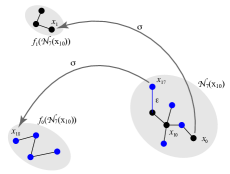
Given a time series that we suspect to be generated by an IFS, the detection and separation algorithm requires an appropriate value for . Here we outline a possible algorithm.
-
•
(Detection) Determine a value for by computing histograms of the separations between and . If is sampled from a connected invariant set, then each of the nearest neighbor sets should be -connected. If there is more than one regime, their images should be disconnected for some choice of . The number of regimes is estimated to be the number of components in the majority of the ; this should be persistent over a range of and values.
-
•
(Separation) Select a set of -nearest-neighborhoods, , that overlap and cover . Points are identified to be from a common regime if they lie in overlapping neighborhoods and their images lie in -connected components.
In the next section, we illustrate this method on a simple example.
III Example: a Hénon IFS
As a simple example, consider the IFS generated by the two quadratic, planar diffeomorphisms
| (3) |
The map is Hénon’s quadratic map with the canonical choice of parameter values Hénon (1976); the map is conjugate, via an affine change of coordinates, to Hénon’s map with parameters . We generate a single trajectory of this IFS by using a Bernoulli process with equal probability to generate a sequence . A trajectory with points, shown in Fig. 2, has the appearance of two overlapping Hénon-like attractors. Note however, that since most points on are not iterated more than a couple of consecutive steps with the same map, is not just the union of the attractors of and . Indeed the attractor for is simply a fixed point at .
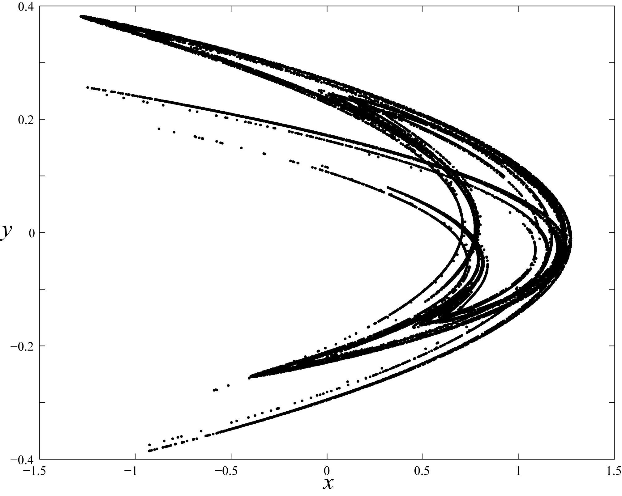
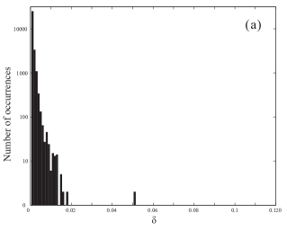
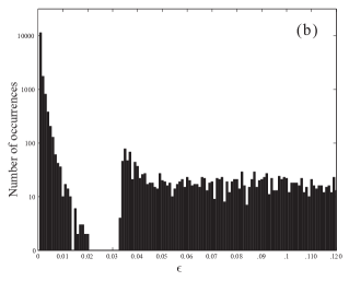
To recover the regime sequence from we must check for -disconnected images of -connected components. As a first step to determine an appropriate value for , we compute the distance between each point in and its nearest neighbor, i.e., the diameter of . This is shown in panel (a) of Fig. 3 as a histogram. Note that all but two points in have a nearest neighbor within , and the vast majority within . Panel (b) of Fig. 3 indicates how these distances grow upon iteration: it shows the distance between the iterates of each of these nearest neighbors, i.e., the diameter of . There are now two distinct distributions separated by a gap . This suggests that the dynamics underlying is discontinuous, and that a choice of in the gap may be appropriate.
Suppose that we did not know that the IFS (3) had two regimes—that only the trajectory of Fig. 2 was available. To detect the number of regimes, we look at the number of -components in the image of the sets of five nearest-neighbors, . Histograms of the number of -components of are shown in Fig. 4 as varies from to . The vast majority of these neighborhoods split into at most two -components. When is as small as about 3% split into four or more components and when , only 0.3% split into three or more components. Note that with the equal probability rule that we used for (3), the probability that all five points in will be iterated with the same map is , which is confirmed in Fig. 4, since about 6% of the images have one -component.
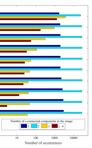
Thus in the detection phase of the algorithm, we confirm that the underlying dynamics has two regimes, and obtain a reasonable choice, .
For the separation phase of the algorithm, we wish to classify which points on are images of which map. To do this we choose larger, overlapping neigbhorhoods that cover so that we can connect the subsets for each regime. To distribute these neigbhorhoods, more-or-less evenly over , we select points by first choosing arbitrarily, and subsequently incrementing and selecting to be the point of farthest from the previously selected points. Each selected point is the nexus of the -nearest-neighborhood
We choose and , so that most of the overlap with other neighborhoods, in the sense that they share points in . In this case, each of the is -connected.
The separation into regimes is accomplished as follows: whenever two “overlapping” ’s have -connected image components that intersect, we identify them as being generated by the same ; see the sketch in Fig. 5. More specifically, suppose that is the set of points in that generate the -component of . These are distinguished by the following: whenever , then the union of their images will share a point as well, and thus be -connected. In this case, the points in these images are selected as being generated by the same regime . That is, for .
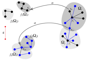
The can be thought of as nodes on an abstract graph. Whenever two of these neighborhoods share a point, an edge linking these nodes is added to the graph. Using this construction, the connected components of the resulting graph are selected as images of a fixed regime. Of course, we do not know which of the ’s is associated with which graph component unless we have prior knowledge of some values of the functions.
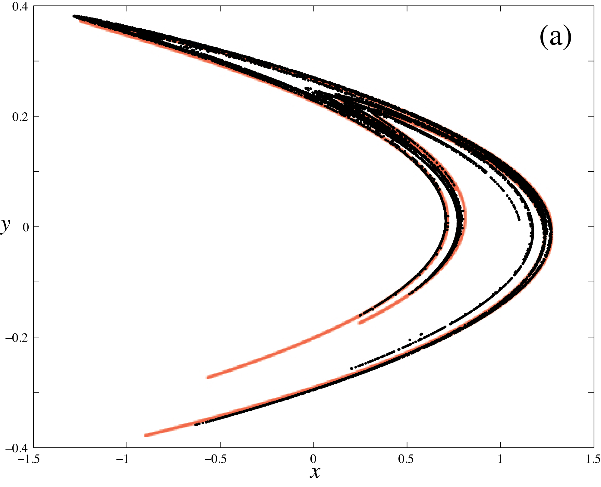
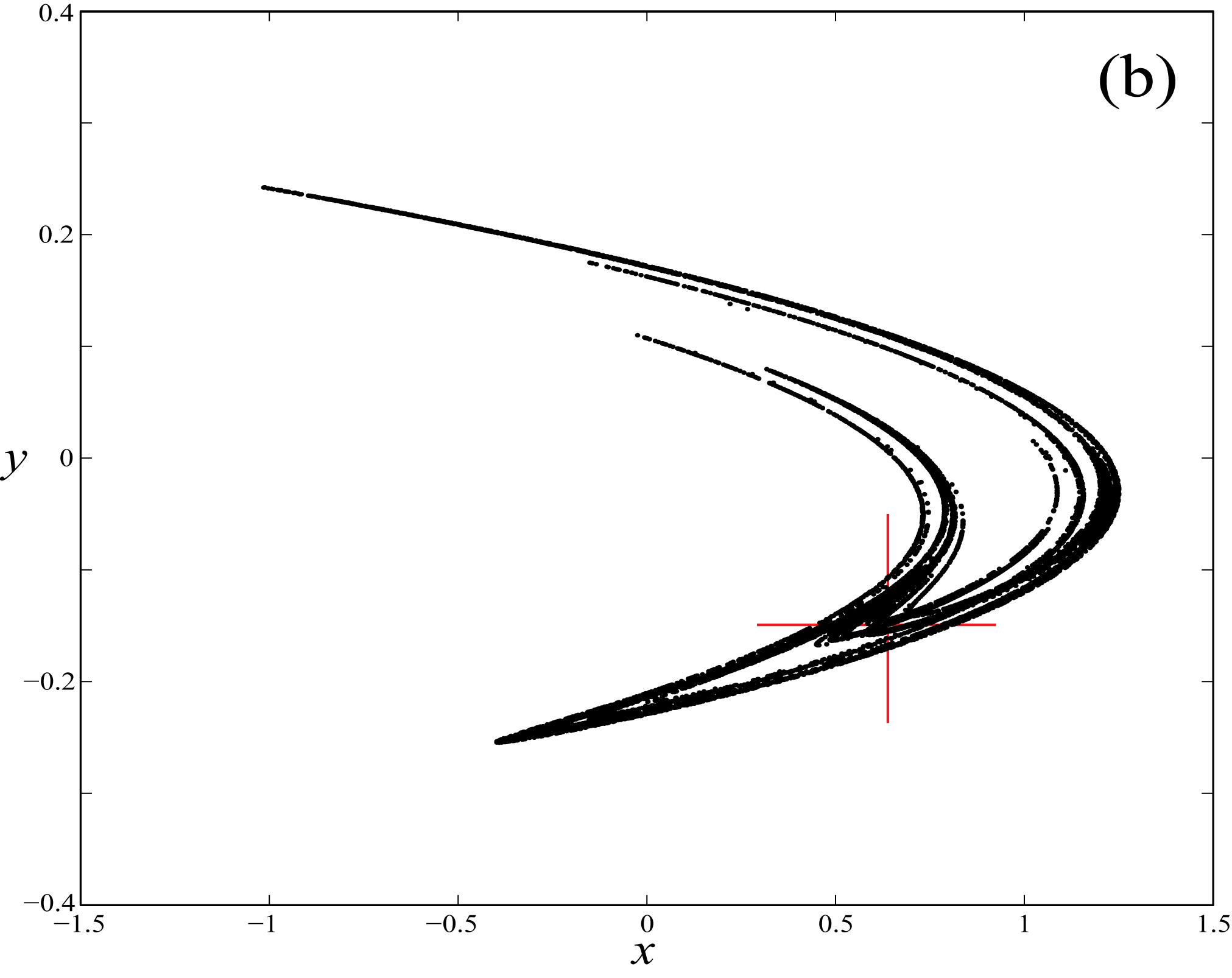
For the trajectory of Fig. 2 and using the covering by the neighborhoods , this algorithm generates two large connected graph components, one containing points and the other points. These sets of points are shown in the panels (a) and (b) of Fig. 6, respectively. Comparing these results with the known values of shows that every point in the first graph component has and every point in the second has ; that is, both the separation had no false positives. There are an additional points of that are not in these two graph components. These unidentified points represent sparsely visited regions of the trajectory.
It is no coincidence that the points identified to be images of in Fig. 6(a) appear to lie close to the attractor of the standard Hénon map, which is shown in grey (light red, online) in the figure. Note, however, that even though the attractor for is a fixed point—the cross in the figure—the strong perturbation due to iterations causes the points in Fig. 6(b) to range far from the attractor of .
IV Computer Performance Dynamics
In this section, we describe the application of the regime separation algorithm to a time series obtained from an experimentally obtained computer performance analysis data set. A critical performance bottleneck in modern computer systems occurs in the efficient management of memory. The cache is the level of memory closest to the processor; it is preloaded with the data that the system thinks it will need. When the system looks for a necessary piece of data in the cache and does not find it, it must load the data from main memory, resulting in a major performance slowdown. Such an event is called a cache miss.
The experiment to investigate the frequency of cache misses consists of repeatedly running the simple C program:
on an Intel Core2® processor. This code initializes the upper triangular portion of a matrix in row-major order. As the program runs, the hardware performance monitors built into the processor monitor the memory usage patterns—in particular, the rate of cache misses. The program is interrupted every instructions and the number of cache misses that occurred over that interval is recorded. We obtained a time series consisting of 86,107 points, from which we used a representative 60,000 point segment for the work presented in this paper. A snippet of the time series, along with the first return map of the 60,000 points selected is shown in Fig. 7. This data set has been studied previously and shown to exhibit chaotic dynamics Alexander et al. (2010); Mytkowicz, Diwan, and Bradley (2009).
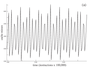
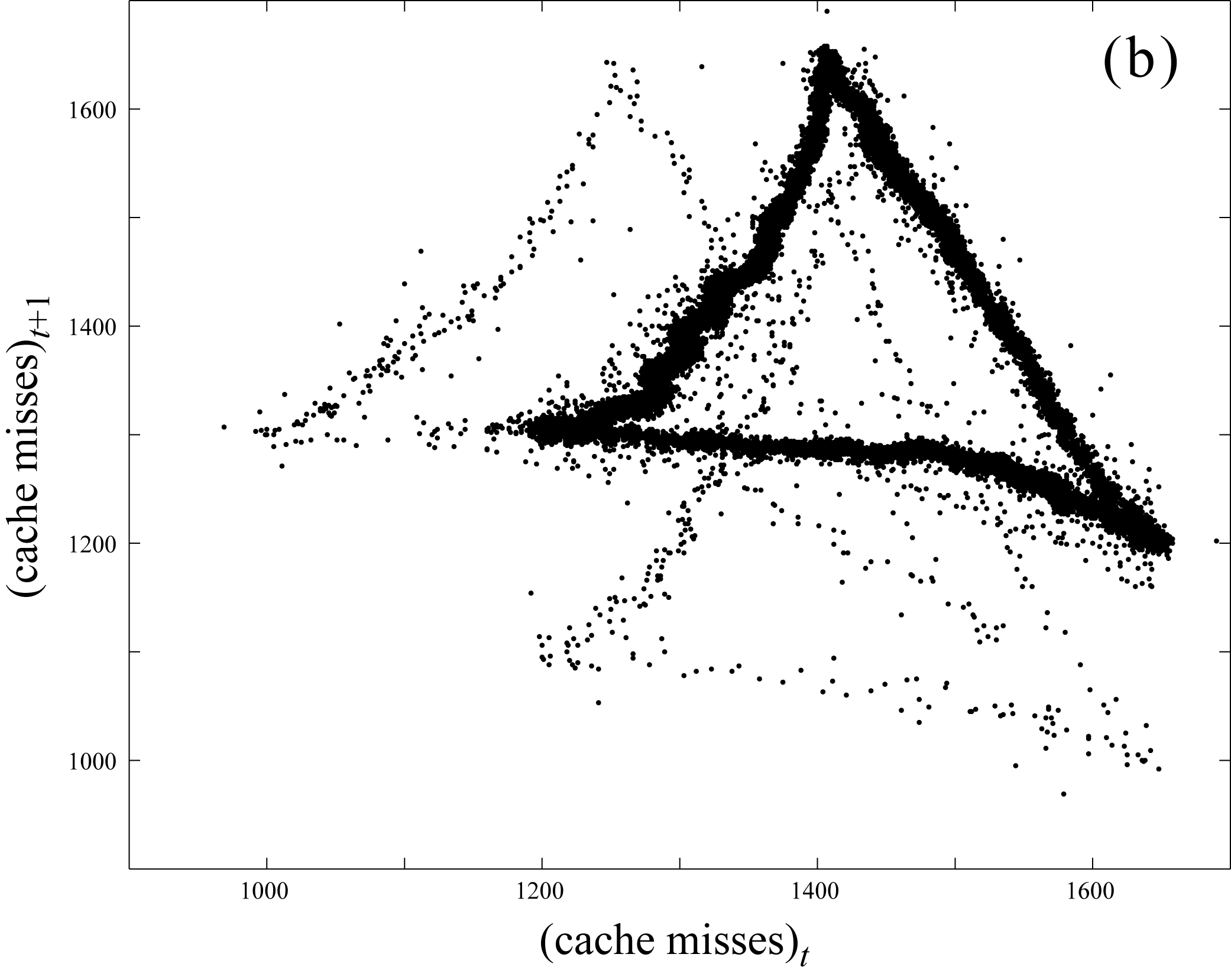
The time delay embedding process we use to analyze the computer performance trace involves the estimation of two parameters: the time delay and the embedding dimension . We first choose using standard practices Sauer, Yorke, and Casdagli (1991); Takens (1981). Based on the first minimum of the time-delayed average mutual information we choose instructions. After choosing the delay , the next step in the embedding process is to estimate the dimension . A standard strategy for this is the “false nearest neighbor” approach of Abarbanel and KennelAbarbanel and Kennel (1993). Based on this algorithm, we estimate that , then narrow down that range to using other dynamical invariants Mytkowicz, Diwan, and Bradley (2009). Note that the first return map shown in Fig. 7 is simply a two-dimensional projection of the 12-dimensional state space embedding, . For a more detailed discussion of these choices and our approach to estimating them see Garland and BradleyGarland and Bradley (2011) or Mytkowicz, et al.Mytkowicz, Diwan, and Bradley (2009).
The observation of the ghost triangles in Fig. 7—seemingly reminiscent of three overlapping attractors from an IFS—prompted us to apply our regime-separation algorithm to this data. Because the two ghosts are much more lightly sampled than the “main” triangle, our conjecture was that the IFS consisted of three functions and that the switching process prioritized one of the three.
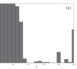
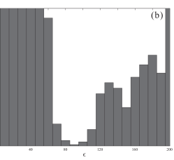
For the analysis, we chose . This choice is justified by observation of the histograms shown in Fig. 8. Figure 8(a) is the histogram of the distances between each point in the time-series embedding and its nearest neighbor, i.e., the diameter of in . Figure 8(b), shows the histogram of distances between the same two points after iterating them both forward one time step, i.e., the diameter of . The two ‘humps’ indicate that, for a generic pair of nearest neighbors, the images of those neighbors are either within of each other (iterates of the same ), or further than apart (iterates of different ).
We separated the ghosts as follows: For each , we examine the image of and its nine nearest neighbors. That is, if consists of two -connected components, then we identify the members of the smaller component (in cardinality) as candidates for points on the ghost triangle. Hence, we have a sequence such that is identified as a point on the ghost for . These points correspond to the lower ghost of Fig. 7; the second ghost is just an image of the first—a necessary result of the symmetry inherent in the time-delay embedding process. Furthermore, we note that the occurrence of ghost points is strongly periodic, with a period of 215 measurements. This claim is motivated by the plot in Fig. 9. This plot is the first difference of the sequence , i.e., the point indicates that the ghost occurs measurements after the ghost. Furthermore, the points on this graph that fall below the line are the result of an ‘extra’ identification in the middle of a period. For example, the first two such points have coordinates and . Since , one might hypothesize that the ghost identification is actually spurious.

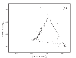
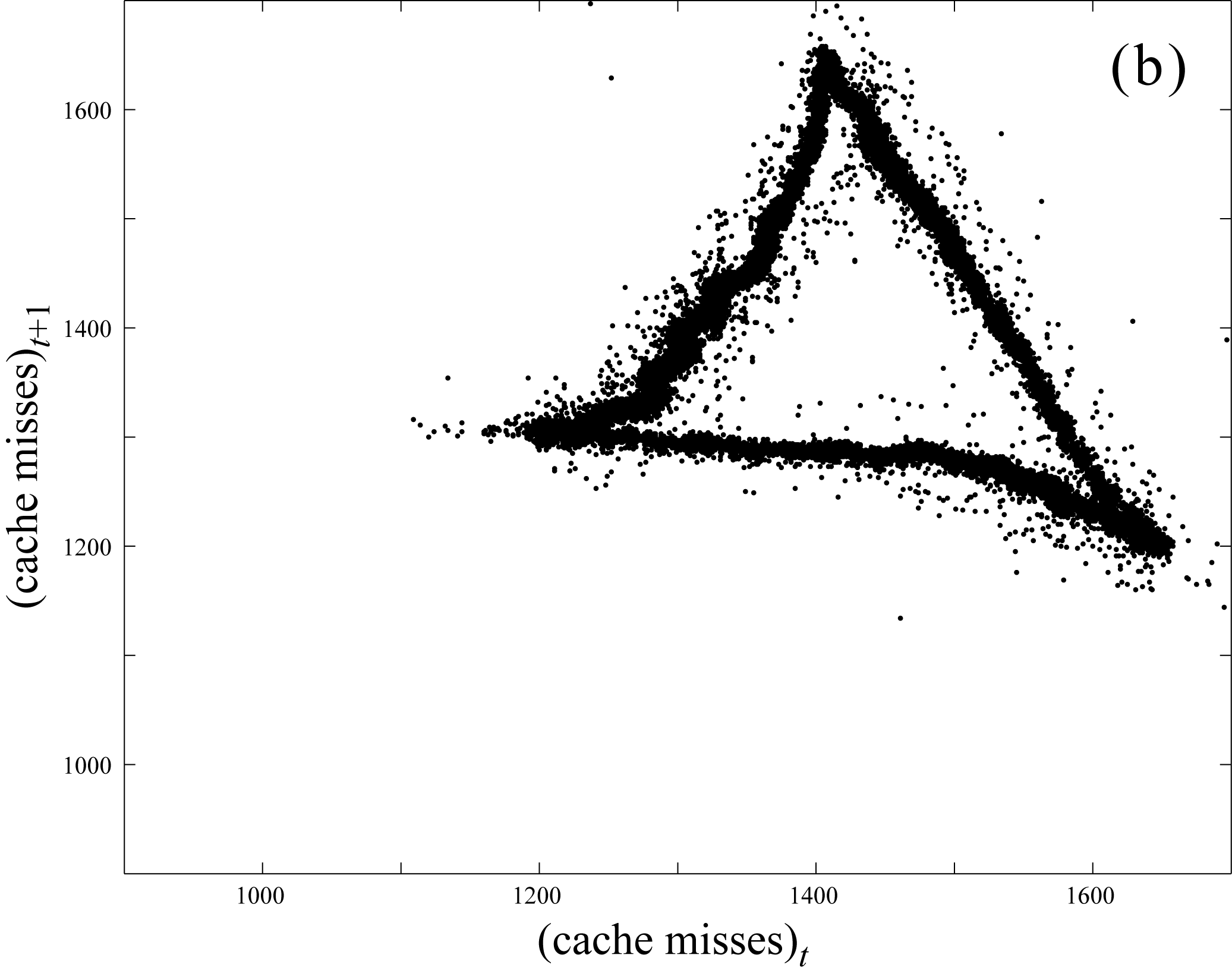
This analysis reinforces the hypothesis that there is a direct correspondence between the points on the ghosts and points in the time series that are periodically spaced by 215 measurements. Moreover, each ghost point appears to be shifted exactly 200 cache misses from the main triangle. Indeed, adding cache misses to each of the points identified as parts of a ghost triangle, produces a time series that has the embedding shown in Fig. 10. Thus, for this case, not only is the regime identified, but the dynamics of the two components is shown to be simply related: by just a shift.
There is one issue remaining before we can model this data as an IFS: we only have access to measurements of the states of the IFS. That is, if is the state space of the computer system and is a collection of maps on , the observations correspond to the functions with a continuous measurement function that maps the state of the computer system to the number of cache misses that occur over the given time interval. It can be shown that the functions are sufficient for studying topological and geometric properties of the ; a more-detailed treatment of the function can be found in Alexander et al.Alexander et al. (2010).
Thus, if denotes the dynamics associated with the main triangle, we can define , and , where . The IFS consists of the state space , the collection of continuous maps, and the sequence , where
This model of the the cache-miss dynamics on the Intel Core2® rests on the assumption that and can be described completely in terms of . To verify this assumption, we tested for determinism in the adjusted dynamical system of Fig. 10. We found that out of the 295 points so identified, only 16 failed to lie in an -connected image set in the adjusted dynamical system. Consequently, appears to be a continuous function and the IFS is an accurate model for this data set.
Much of the usefulness of this model originates from the fact that we have isolated the continuous function . In light of this, it is reasonable to assume that is representative of some low-dimensional dynamics that are present in the computer system, while and represent a secondary piece of dynamics—in this case, perhaps best described as ‘deterministic additive noise’.
V Conclusion
Many techniques for time-series analysis, such as in Mischaikow et al.Mischaikow et al. (1999), explicitly require the time series to be generated by a continuous function, and almost all of them implicitly require that it be generated by a single function. For example, in Mytkowicz et al. Mytkowicz, Diwan, and Bradley (2009), time-series analysis of the data of Fig. 7 showed that it has a positive Lyapunov exponent and fractal correlation dimension. However, our results show that that time series interleaves trajectories from different dynamical systems—a property that can trip up traditional time-series analysis techniques. In the data studied in Mytkowicz et al. Mytkowicz, Diwan, and Bradley (2009), this proved not to be an issue because a single overwhelmingly dominated the dynamics. When that is not the case, problems can arise with traditional methods, which are often formulated assuming the existence of long, uninterrupted deterministic trajectories. Some techniques, such as those in Mischaikow et al.Mischaikow et al. (1999), do not explicitly require uninterrupted trajectories. Using our topology-based approach, one could pull apart the time-series data into individual regimes and study the dynamics of each of the independently.
In conclusion, we have described an algorithm for detection and separation of a signal that is generated by continuous, deterministic dynamics punctuated by regime shifts. The algorithm handles shifts that result from stochastic or deterministic processes: it applies whenever the dynamics are described by an iterated function system. Time-series data from a computer performance analysis experiment were shown to fit this model. More generally, we claim that iterated function systems are a natural model for complex computer programs, which—we hypothesize—have regime shifts as their execution moves through different parts of the code.
IFS models provide a natural framework for data analysis in a wide range of fields: whenever the physical system generating the data is characterized by continuous systems, that are punctuated by discontinuous regime shifts. Another area in which the regime separation technique is particularly appropriate is digital communication channels. Indeed, (hyperbolic) iterated function systems are known to provide useful models of these channels Broomhead et al. (2004). A channel corresponds to an electrical circuit externally driven by a digital signal, and the discrete input signal corresponds to the regime sequence. Thus, the behavior of the circuit corresponds to the actions of a discrete set of continuous dynamical systems. A fundamental problem in this context is channel equalization, the reversal of distortion that is incurred by transmission through a channel. This is precisely the determination of the input signal sequence from a sequence of output values—i.e., regime separation. Channel equalization is straightforward for linear dynamics because the IFS attractors in these situations tend to be non-overlapping. However, more-realistic, nonlinear IFS models have overlapping attractors. We believe that our methods can be successfully used for channel equalization in this context.
Challenges that remain to be addressed include finding an efficient implementation for high-dimensional data and dealing with systems that have traditional (e.g. Gaussian) noise in addition to regime shifts. Furthermore, we have not addressed the nature of the switching process itself. Once the regime shifts have been determined, the next natural question to ask is whether or not the switching is deterministic or stochastic, and if one can determine the rule for switching between regimes.
References
- Theiler et al. (1992) J. Theiler, S. Eubank, A. Longtin, B. Galdrikian, and J. Farmer, “Testing for nonlinearity in time series: the method of surrogate data,” Physica D 58, 77–94 (1992).
- Sugihara and May (1990) G. Sugihara and R. May, “Nonlinear forcasting as a way of distinguishing chaos from measurement error in time series,” Nature 344, 734–740 (1990).
- Diaconis and Freedman (1999) P. Diaconis and D. Freedman, “Iterated random functions,” SIAM review , 45–76 (1999).
- Broomhead et al. (2004) D. Broomhead, J. Huke, M. Muldoon, and J. Stark, “Iterated function system models of digital channels,” Proc. Roy. Soc. London. Series A 460, 3123 (2004).
- Kawahara and Sugiyama (2009) Y. Kawahara and M. Sugiyama, “Change-point detection in time-series data by direct density-ratio estimation,” in Proceedings of 2009 SIAM International Conference on Data Mining (SDM2009) (2009) pp. 389–400.
- Kaplan and Shishkin (2000) A. Kaplan and S. Shishkin, “Application of the change-point analysis to the investigation of the brain’s electrical activity,” Nonparametric Statistical Diagnosis: Problems and Methods , 333–388 (2000).
- Klonowski et al. (1999) W. Klonowski, W. Jernajczyk, K. Niedzielska, A. Rydz, and R. Stepien, “Quantitative measure of complexity of EEG signal dynamics,” Acta Neurobiologiae Experimentalis 59, 315–322 (1999).
- Glass and Kaplan (1993) L. Glass and D. Kaplan, “Time series analysis of complex dynamics in physiology and medicine,” Medical Progress Through Technology 19, 115–115 (1993).
- Turchin and Taylor (1992) P. Turchin and A. Taylor, “Complex dynamics in ecological time series,” Ecology 73, 289–305 (1992).
- Chen (1988) P. Chen, “Empirical and theoretical evidence of economic chaos,” System Dynamics Review 4, 81–108 (1988).
- Barnsley (1988) M. Barnsley, Fractals Everywhere (New York: Academic Press, 1988).
- Falconer (2003) K. Falconer, Fractal Geometry: Mathematical Foundations and Applications (John Wiley, 2003).
- Sauer, Yorke, and Casdagli (1991) T. Sauer, J. Yorke, and M. Casdagli, “Embedology,” Journal of Statistical Physics 65, 579–616 (1991).
- Takens (1981) F. Takens, “Detecting strange attractors in turbulence,” in Dynamical Systems and Turbulence, Warwick 1980, Lecture Notes in Mathematics, Vol. 898, edited by D. Rand and L.-S. Young (Springer Berlin / Heidelberg, 1981) pp. 366–381.
- Robins, Meiss, and Bradley (2000) V. Robins, J. Meiss, and E. Bradley, “Computing connectedness: Disconnectedness and discreteness,” Physica D 139, 276–300 (2000).
- Hénon (1976) M. Hénon, “A two-dimensional mapping with a strange attractor,” Comm. Math. Phys. 50, 69–77 (1976).
- Alexander et al. (2010) Z. Alexander, T. Mytkowicz, A. Diwan, and E. Bradley, “Measurement and dynamical analysis of computer performance data,” Adv. in Intelligent Data Analysis IX , 18–29 (2010).
- Mytkowicz, Diwan, and Bradley (2009) T. Mytkowicz, A. Diwan, and E. Bradley, “Computer systems are dynamical systems,” Chaos 19, 033124 (2009).
- Abarbanel and Kennel (1993) H. Abarbanel and M. Kennel, “Local false nearest neighbors and dynamical dimensions from observed chaotic data,” Physical Review E 47, 3057 (1993).
- Garland and Bradley (2011) J. Garland and E. Bradley, “Predicting computer performance dynamics,” in Advances in Intelligent Data Analysis X (Springer Lecture Notes in Computer Science, 2011).
- Mischaikow et al. (1999) K. Mischaikow, M. Mrozek, J. Reiss, and A. Szymczak, “Construction of symbolic dynamics from experimental time series,” Physical Review Letters 82, 1144–1147 (1999).