Strongly scale-dependent polyspectra from curvaton self-interactions

Abstract:

We study the scale dependence of the non-linearity parameters $f_{\rm NL}$ and $g_{\rm NL}$ in curvaton models with self-interactions. We show that the spectral indices $n_{f_{\rm NL}}={\rm d}\,{\rm ln}|f_{\rm NL}|/{\rm d}\,{\rm ln}\,k$ and $n_{g_{\rm NL}}={\rm d}\,{\rm ln}|g_{\rm NL}|/{\rm d}\,{\rm ln}\,k$ can take values much greater than the slow–roll parameters and the spectral index of the power spectrum. This means that the scale–dependence of the bi and trispectrum could be easily observable in this scenario with Planck, which would lead to tight additional constraints on the model. Inspite of the highly non-trivial behaviour of $f_{\rm NL}$ and $g_{\rm NL}$ in the curvaton models with self-interactions, we find that the model can be falsified if $g_{\rm NL}(k)$ is also observed.

1 Introduction

Non-Gaussianity of the primordial perturbations can efficiently discriminate between different models of inflation. It is by now well known that both the strength and statistical properties of primordial non-Gaussianities depend crucially on the details of the inflationary model. While conventional slow roll models of inflation with canonical dynamics typically predict negligible non-Gaussianity, non-minimal constructions may generate observable non-Gaussianity. For a selection of recent reviews see [1, 2, 3, 4, 5]. Examples of such scenarios include models with non-canonical kinetic terms or a breakdown of slow roll dynamics and models where the primordial perturbations are generated at the end of inflation, like in modulated reheating [6, 7], or after the end of inflation, like in the curvaton scenario [8, 9].

The simplest type of non-Gaussianity is the so called local form. The local Ansatz for the primordial curvature perturbation reads

$$\zeta_{{\bf k}}=\zeta^{{\rm G}}_{{\bf k}}+\frac{3}{5}f_{\rm NL}(\zeta^{{\rm G}}\star\zeta^{{\rm G}})_{{\bf k}}+\frac{9}{25}g_{\rm NL}(\zeta^{{\rm G}}\star\zeta^{{\rm G}}\star\zeta^{{\rm G}})_{{\bf k}}\ ,$$ (1)

where $\zeta^{{\rm G}}$ is a Gaussian field and the non-linearity parameters $f_{\rm NL}$ and $g_{\rm NL}$ are constants. The star denotes a convolution. In [10, 11] it was shown that non-linearities of the field equations in general give rise to a mild scale dependence of $f_{\rm NL}$ and $g_{\rm NL}$ even in models with canonical slow-roll dynamics during inflation, which typically have been analyzed using the local Ansatz. Deviations from the local Ansatz were analyzed previously from an observational point of view in [12, 13] and more recently in [14, 15]. The scale dependence of $f_{\rm NL}$ and $g_{\rm NL}$ can be described by the quantities

$$n_{f_{\rm NL}}=\frac{{\rm d}\,{\rm ln}|f_{\rm NL}|}{{\rm d}\,{\rm ln}\,k}\ ,\qquad n_{g_{\rm NL}}=\frac{{\rm d}\,{\rm ln}|g_{\rm NL}|}{{\rm d}\,{\rm ln}\,k}\ ,$$ (2)

and in models with slow roll dynamics during inflation the typical magnitude of $n_{f_{\rm NL}}$ and $n_{g_{\rm NL}}$ is set by slow roll parameters [11]. Hence the local Ansatz (1) gets replaced by a quasi-local form with $f_{\rm NL}$ and $g_{\rm NL}$ being weakly $k$-dependent functions. Although the scale dependence is typically weak (for an exception see [16]), it could be an observable effect which makes this topic very interesting. This topic is also interesting in models of non–local Gaussianity, see e.g. [17, 18, 19, 20].

In this work we compute the scale dependency of the non-linearity parameters in self-interacting curvaton models. The scale dependence in the limit of weak interactions, where the self-interaction does not dominate over the quadratic part in the curvaton potential, was considered already in [21]. Here we analyze also the self-interaction dominated regime, which turns out to be particularly interesting. In this regime the non-linearity parameters $f_{\rm NL}$ and $g_{\rm NL}$ depend sensitively on the curvaton value at the time of inflation [22, 23, 24, 25, 26]. In particular, they oscillate around the naive estimates $|f_{\rm NL}|\sim r_{\rm dec}^{-1}$ and $|g_{\rm NL}|\sim r_{\rm dec}^{-2}$, where $r_{\rm dec}$ denotes the curvaton contribution to the total energy density at the decay time. We find that the non-linearity parameters become strongly scale-dependent in the regions $|f_{\rm NL}|\ll r_{\rm dec}^{-1},|g_{\rm NL}|\ll r_{\rm dec}^{-2}$. For small values of $r_{\rm dec}$ the non-Gaussian effects in these regions are at the observable level and the scale dependence will be a detectable feature of this model in the near future. We also comment on how the results could be generalized to any models where the primordial perturbation arises from a component which is subdominant during inflation.

The paper is organized as follows: in Section 2 we review the self-interacting curvaton scenario to the extent needed in our analysis. In Section 3 we derive expressions for the scale dependent non-Gaussianity in the curvaton scenario and discuss their generic features. In Section 4 we discuss the case of quartic self–interactions, deriving both analytical and numerical results. In Section 5, we discuss the scale dependence in curvaton models with non-renormalizable self-interactions, while in Section 5.1 we study the regime of very large self interactions and find an analytical approximation. Finally, we present our conclusions in Section 6. We use the units $M_{\rm P}=(8\pi G)^{-1/2}=1$ throughout the paper.

2 Self-interacting curvaton model

We consider self-interacting curvaton models where the curvaton potential is given by

$$V=\frac{1}{2}m^{2}\sigma^{2}+\lambda\sigma^{n}\ ,$$ (3)

where $n=4,6,8$.

While the curvaton should oscillate before decaying, and the quadratic part will typically be dominant at this stage due to the small field value, the self-interacting part may play an important role at earlier stages, crucially affecting the predictions of the curvaton scenario [22, 23, 24, 25, 26, 27, 28, 29, 30, 31, 32]. We assume the primordial perturbation arises solely from the fluctuations of the curvaton field $\sigma$ and neglect the inflaton contribution. Mixed scenario’s were considered in [33]. After the end of inflation the inflaton decays into radiation which dominates the universe. We assume the curvaton decays instantaneously into radiation at $H_{\rm dec}=\Gamma$, for a discussion on the accuracy of this approximation see [34, 35]. If the curvaton is coupled to other scalars, it may also decay non-perturbatively through a parametric resonance [36, 37], we will not consider this possibility here.

Using the $\delta N$ formalism [38, 39, 40, 41, 42], the curvature perturbation can be expressed in the form

$$\zeta_{{\bf k}} = N^{\prime}(t_{k})\delta\sigma_{{\bf k}}(t_{k})+\frac{1}{2}N^{\prime\prime}(t_{k})(\delta\sigma\star\delta\sigma)_{{\bf k}}(t_{k})+\frac{1}{6}N^{\prime\prime\prime}(t_{k})(\delta\sigma\star\delta\sigma\star\delta\sigma)_{{\bf k}}(t_{k})+\ldots$$ (4)

$$= \frac{2\,r_{\rm dec}}{3}\frac{\sigma_{\rm osc}^{\prime}}{\sigma_{\rm osc}}\delta\sigma_{{\bf k}}(t_{k})+\frac{r_{\rm dec}}{3}\left(\frac{\sigma_{\rm osc}^{\prime\prime}}{\sigma_{\rm osc}}+\left(\frac{\sigma_{\rm osc}^{\prime}}{\sigma_{\rm osc}}\right)^{2}\right)(\delta\sigma\star\delta\sigma)_{{\bf k}}(t_{k})$$

$$+\frac{r_{\rm dec}}{9}\left(\frac{\sigma_{\rm osc}^{\prime\prime\prime}}{\sigma_{\rm osc}}+3\frac{\sigma_{\rm osc}^{\prime\prime}\sigma_{\rm osc}^{\prime}}{\sigma_{\rm osc}^{2}}\right)(\delta\sigma\star\delta\sigma\star\delta\sigma)_{{\bf k}}+\cdots\,,$$

where the convolutions are defined by $(\delta\sigma\star\delta\sigma)_{{\bf k}}(t_{k})=(2\pi)^{-3}\int{\rm d}{\bf q}\,\delta\sigma_{{\bf q}}(t_{k})\delta\sigma_{{\bf k}-{\bf q}}(t_{k})$. $N(t_{k})$ denotes the number of e-foldings from an initial spatially flat hypersurface $t_{k}$, corresponding to the horizon exit of the mode $k$, to some final uniform energy density surface after the decay of the curvaton. The primes denote derivatives with respect to $\sigma(t_{k})$. $\sigma_{\rm osc}$ sets the scale of the curvaton envelope during the final quadratic oscillations before the decay, $\bar{\sigma}(t)=\sigma_{\rm osc}/(mt)^{3/4}$, see equation (9) below. $r_{\rm dec}$ measures the curvaton contribution to the total energy density at the time of decay,

$$r_{\rm dec}=\frac{3}{4}\frac{\rho_{\sigma}}{3H^{2}}\Big{|}_{\rm dec}\simeq\frac{1}{2\sqrt{2}}\,\sigma_{\rm osc}^{2}\left(\frac{m}{\Gamma}\right)^{1/2}\ ,$$ (5)

and the results are computed to first order in $r_{\rm dec}$ throughout this work.

The information about curvaton self-interactions in (4) is essentially encoded into the derivatives of $\sigma_{\rm osc}$. In general, it is not possible to compute $\sigma_{\rm osc}(\sigma(t_{k}))$ analytically. However, we can obtain some generic information by just looking at the evolution equation for the curvaton field in the radiation dominated epoch,

$$\ddot{\sigma}+\frac{3}{2t}\dot{\sigma}+m^{2}\sigma+n\lambda\sigma^{n-1}=0\ .$$ (6)

Switching to the variable $x=mt$ and writing $\sigma=\sigma(t_{k})\xi(x)x^{-3/4}$, we obtain

$$\frac{{\rm d}^{2}\xi}{{\rm d}x^{2}}+\xi(1+\frac{3}{16}x^{-2})+\frac{ns}{2}\,\xi^{n-1}x^{-3(n-2)/4}=0\ .$$ (7)

Here we have defined a (relative) self-interaction strength parameter $s$ by

$$s=\frac{2\,\lambda\sigma(t_{k})^{n-2}}{m^{2}}\ ,$$ (8)

which is simply the ratio of potential energies stored in the curvaton self-interactions and the bare mass part in (3). Beware that various definitions of $s$ and $r_{\rm dec}$ have been used in the literature.

In the asymptotic limit $x\rightarrow\infty$, corresponding to the regime of quadratic oscillations, (7) has a solution $\xi_{\rm as}=\hat{\sigma}_{\rm osc}(s)\,{\rm sin}(x+\varphi(s))$, and we obtain the asymptotic result

$$\sigma_{\rm as}(t)=\sigma(t_{k})\hat{\sigma}_{\rm osc}(s)\frac{{\rm sin}(mt+\varphi(s))}{(mt)^{3/4}}\equiv\sigma_{\rm osc}\frac{{\rm sin}(mt+\varphi(s))}{(mt)^{3/4}}\ .$$ (9)

From this we learn that $\sigma_{\rm osc}$ can be expressed in the form

$$\sigma_{\rm osc}(\sigma(t_{k}))=\sigma(t_{k})\hat{\sigma}_{\rm osc}(s)\ .$$ (10)

3 Scale-dependent non-Gaussianity

We analyze the scale-dependence of the non-linearity parameters using the formalism developed in [10, 11]. The curvaton perturbations at horizon crossing, $\delta\sigma_{{\bf k}}(t_{k})$, are assumed to be Gaussian. We study the effect of relaxing this assumption in Appendix A. We denote the Gaussian part of the curvature perturbation (4) by

$$\zeta_{{\bf k}}^{{\rm G}}\equiv N^{\prime}(t_{k})\delta\sigma_{{\bf k}}(t_{k})\equiv\frac{2\,r_{\rm dec}}{3}z(s)\frac{\delta\sigma_{{\bf k}}(t_{k})}{\sigma(t_{k})}\ ,$$ (11)

where the function $z(s)$ is given by

$$z(s)=\frac{\sigma(t_{k})\sigma_{\rm osc}^{\prime}}{\sigma_{\rm osc}}=1+\frac{(n-2)s}{\hat{\sigma}_{\rm osc}}\frac{\partial\hat{\sigma}_{\rm osc}}{\partial s_{~{}~{}~{}}}\ .$$ (12)

The expression (4) for the curvature perturbation can now be written as

$$\zeta_{{\bf k}}=\zeta_{{\bf k}}^{{\rm G}}+\frac{3}{5}f_{\rm NL}(k)(\zeta^{{\rm G}}\star\zeta^{{\rm G}})_{{\bf k}}+\frac{9}{25}g_{\rm NL}(k)(\zeta^{{\rm G}}\star\zeta^{{\rm G}}\star\zeta^{{\rm G}})_{{\bf k}}+\cdots\ ,$$ (13)

where the non-linearity parameters are given by

$$f_{\rm NL}(k) = \frac{5}{6}\frac{N^{\prime\prime}(t_{k})}{N^{\prime}(t_{k})^{2}}=\frac{5}{4r_{\rm dec}}\left(1+\frac{\sigma_{\rm osc}^{\prime\prime}\sigma_{\rm osc}}{\sigma_{\rm osc}^{\prime}{}^{2}}\right)\equiv\frac{5}{4r_{\rm dec}}\,f(s)\ ,$$ (14)

$$g_{\rm NL}(k) = \frac{25}{54}\frac{N^{\prime\prime\prime}(t_{k})}{N^{\prime}(t_{k})^{3}}=\frac{25}{24r_{\rm dec}^{2}}\left(\frac{\sigma_{\rm osc}^{\prime\prime\prime}\sigma_{\rm osc}^{2}}{\sigma_{\rm osc}^{\prime}{}^{3}}+\frac{3\sigma_{\rm osc}^{\prime\prime}\sigma_{\rm osc}}{\sigma_{\rm osc}^{\prime}{}^{2}}\right)\equiv\frac{25}{24r_{\rm dec}^{2}}\,g(s)\ ,$$ (15)

to leading order in $r_{\rm dec}$. Since we assume $\zeta$ is generated by a single field, the third non-linearity parameter $\tau_{\rm NL}$, describing the trispectrum together with $g_{\rm NL}$, is uniquely determined by $f_{\rm NL}$

$$\tau_{\rm NL}=\left(\frac{6}{5}f_{\rm NL}\right)^{2}\ .$$

It hence trivially follows that $n_{\tau_{\rm NL}}=2n_{f_{\rm NL}}$, as is always the case for a model where $\zeta$ is generated by a single-source [11]. For a general discussion of the relation between the (local) non-linearity parameters see [43].

Information about the curvaton interactions is encoded into the functions $f(s)$ and $g(s)$, which depend only on the self-interaction strength parameter $s$. For a purely quadratic model, $s=0$, they read $f=1$ and $g=0$ since $\sigma_{\rm osc}\propto\sigma(t_{k})$. In the presence of self-interactions, $f(s)$ and $g(s)$ become non-trivial functions oscillating between positive and negative values [22]. The level of non-Gaussianity may therefore strongly deviate from the the naive estimates of $|f_{\rm NL}|\sim r_{\rm dec}^{-1}$ and $|g_{\rm NL}|\sim r_{\rm dec}^{-2}$.

Equations (14) and (15) are evaluated at the horizon crossing time $t_{k}$ of the mode $k$ under consideration, which in general makes $f_{\rm NL}$ and $g_{\rm NL}$ scale-dependent [10, 11]. The scale dependence can be described by the parameters $n_{f_{\rm NL}}$ and $n_{g_{\rm NL}}$, which measure logarithmic derivatives of the non-linearity parameters (2). Applying the results of [10, 11] to the curvaton scenario, we find

$$n_{f_{\rm NL}} = \frac{1}{2}\,n_{\tau_{\rm NL}}=\frac{N^{\prime}}{N^{\prime\prime}}\frac{V^{\prime\prime\prime}}{3H^{2}}$$

$$= \frac{\eta_{\sigma}}{f(s)}\left(\frac{n(n-1)(n-2)s}{z(s)(2+n(n-1)s)}\right)\ ,$$

$$n_{g_{\rm NL}} = 3\frac{N^{\prime\prime 2}}{N^{\prime\prime\prime}N^{\prime}}\,n_{f_{\rm NL}}+\frac{N^{\prime}}{N^{\prime\prime\prime}}\frac{V^{\prime\prime\prime\prime}}{3H^{2}}$$

$$= \frac{\eta_{\sigma}}{g(s)}\left(\frac{n(n-1)(n-2)s}{z(s)(2+n(n-1)s)}\left(3f(s)+\frac{n-3}{z(s)}\right)\right)\ .$$

The results are derived to leading order in slow roll, see [10, 11] for details. The functions $z,f,g$ are defined by (12), (14) and (15). The slow–roll parameter $\eta_{\sigma}$ is defined as usual, $\eta_{\sigma}={V^{\prime\prime}}/{(3H^{2})}={m^{2}}(2+n(n-1)s)/({6H^{2}})$. In the curvaton scenario, the scale dependence of $f_{\rm NL}$ and $g_{\rm NL}$ is entirely generated by curvaton interactions. For a purely quadratic model the scale dependence vanishes $n_{f_{\rm NL}}=n_{g_{\rm NL}}=0$ (note that also $r_{\rm dec}^{2}g_{\rm NL}=0$ in this case, subleading corrections in $r_{\rm dec}$ lead to $g_{\rm NL}={\cal O}(f_{\rm NL})$) as the equation of motion for $\sigma$ is fully linear to leading order in $r_{\rm dec}$ [10]. The first detailed study of the scale dependence of $g_{\rm NL}$ for isocurvature models was made in [44].

The results given here are valid for $|n_{f_{\rm NL}}|$ and $|n_{g_{\rm NL}}|$ much less than unity [10, 11]. To discuss stronger scale-dependence, the formalism needs to be modified to account for the non-Gaussianity of the curvaton perturbations $\delta\sigma_{{\bf k}}(t_{k})$. A more detailed discussion on this issue is presented in Appendix A.

3.1 Regimes of enhanced scale-dependence

The complicated dynamics of the self-interacting curvaton scenario can lead to a considerable enhancement of the scale-dependence. In the regions where $|f(s)|\ll 1$ or $|g(s)|\ll 1$, the spectral indices

$$n_{f_{\rm NL}}\propto\frac{\eta_{\sigma}}{f(s)}\ ,\qquad n_{g_{\rm NL}}\propto\frac{\eta_{\sigma}}{g(s)}$$ (18)

can become much larger than the slow-roll scale $\eta_{\sigma}$. The amplitudes $f_{\rm NL}\propto f(s)/r_{\rm dec}$ and $g_{\rm NL}\propto g(s)/r_{\rm dec}^{2}$, on the other hand, depend not only on the self-interaction strength $s$ but also on $r_{\rm dec}$, measuring the curvaton energy density at the time of its decay. As $r_{\rm dec}$ can be varied independently of $s$, the non-linearity parameters $f_{\rm NL}$ and $g_{\rm NL}$ can be large even if $f$ or $g$ are suppressed.

According to [13], Planck should be able to probe the scale-dependence of $f_{\rm NL}$ to the precision

$$\Delta n_{f_{\rm NL}}\simeq 0.1\frac{50}{f_{\rm NL}}\frac{1}{\sqrt{f_{\rm sky}}}\ ,$$ (19)

where $f_{\rm sky}$ stands for the fraction of sky observed and the result is derived taking $f_{\rm NL}=50,n_{f_{\rm NL}}=0$ as fiducial values in the analysis. For CMBpol, the error is expected to be smaller by a factor of two. Since the error $\Delta n_{f_{\rm NL}}$ is inversely proportional to $f_{\rm NL}$, it is also interesting to consider the combination $f_{\rm NL}n_{f_{\rm NL}}\propto\eta_{\sigma}/{r_{\rm dec}}$ for which this dependence drops out. The combination $f_{\rm NL}n_{f_{\rm NL}}$ is parameterically suppressed for $\eta_{\sigma}\ll r_{\rm dec}$ but can become observable for $\eta_{\sigma}\gtrsim r_{\rm dec}$. This is in accordance with our finding that the regions $|f(s)|\ll 1$, with $f(s)$ defined in equation (14), are characterized by an enhanced scale-dependence. Indeed, the lower bound on $r_{\rm dec}$ following from the observational constraint $|f_{\rm NL}|\sim|f(s)|/r_{\rm dec}\lesssim 10^{2}$ [45] gets relaxed in the regions $|f(s)|\ll 1$ which makes it easier to have $\eta_{\sigma}\gtrsim r_{\rm dec}$. For example, if $|f|\simeq 10^{-1}$ then the observational bound on $f_{\rm NL}$ requires that $r_{\rm dec}\gtrsim 10^{-3}$, while the observed value of the spectral index suggests that $\eta_{\sigma}\lesssim 10^{-2}$, and it could be larger if there is an accidental cancellation between $\eta_{\sigma}$ and $\epsilon$. We therefore conclude that there is a reasonably large parameter space in which Planck may be able to detect both the bispectrum and its scale dependence.

A similar enhancement of scale-dependence could also take place in other single-source models where isocurvature perturbations of an initially subdominant field $\chi$ are converted into curvature perturbations at some later stage, and perturbations of the other fields can be neglected. The curvature perturbation can be schematically written in a form analogous to the curvaton case [46], $\zeta=r(\zeta_{\chi}+f(s)\zeta_{\chi}^{2}+\ldots)$, with $r\propto\rho_{\chi}/\rho$ and $s$ measuring interactions of the $\chi$ field. This yields $f_{\rm NL}\propto f(s)/r$ where $r$, being independent of the time of horizon crossing of a given mode, does not contribute to the the scale-dependence. Therefore, $n_{f_{\rm NL}}={{\rm d}\,{\rm ln}|f(s)|}/{{\rm d}\,{\rm ln}\,k}$, and the scale-dependence gets enhanced in the regions $|f|\ll 1$, provided they exist. Similar comments apply to the scale-dependence of $g_{\rm NL}$.

3.2 Running of $n_{f_{\rm NL}}$ and $n_{g_{\rm NL}}$

In the regimes of enhanced scale-dependence, $|n_{f_{\rm NL}}|,|n_{g_{\rm NL}}|\gg\eta_{\sigma}$, the first–order derivatives of $f_{\rm NL}$ and $g_{\rm NL}$ are not necessarily enough to describe the scale-dependence but higher–order derivatives may also become relevant. In addition to $n_{f_{\rm NL}}$ and $n_{g_{\rm NL}}$, one then needs to consider the running of these parameters.

Starting from the expressions (3) and (3) it is straightforward to compute the running of $n_{f_{\rm NL}}$ and $n_{g_{\rm NL}}$ [21, 44]. The results can be expressed in the form

$$\alpha_{f_{\rm NL}}\equiv\frac{{\rm d}\,n_{f_{\rm NL}}}{{\rm d}\,{\rm ln}\,k} = -n_{f_{\rm NL}}^{2}+\left(2\epsilon_{\rm H}-\frac{2(n-2)(1+ns)}{2+n(n-1)s}\,\eta_{\sigma}\right)n_{f_{\rm NL}}\ ,$$ (20)

$$\alpha_{g_{\rm NL}}\equiv\frac{{\rm d}\,n_{g_{\rm NL}}}{{\rm d}\,{\rm ln}\,k} = -n_{g_{\rm NL}}^{2}+\left(2\epsilon_{\rm H}-\frac{2(n-2)(n-3-3ns)}{(n-3)(2+n(n-1)s)}\,\eta_{\sigma}\right)n_{g_{\rm NL}}$$ (21)

$$-\frac{4n^{2}(n-2)s}{(n-3)(2+n(n-1)s)}\frac{f_{\rm NL}^{2}}{g_{\rm NL}}n_{f_{\rm NL}}\eta_{\sigma}\ ,$$

where $\epsilon_{\rm H}=-\dot{H}/H^{2}$.

For $|n_{f_{\rm NL}}|\gg{\cal O}(\eta_{\sigma})$, equation (20) gives $\alpha_{f_{\rm NL}}=-n_{f_{\rm NL}}^{2}+{\cal O}(\epsilon)n_{f_{\rm NL}}$, which implies that ${\rm d}^{2}f_{\rm NL}/{\rm d}\,{\rm ln}\,k^{2}={\cal O}(\epsilon){\rm d}f_{\rm NL}/{\rm d}\,{\rm ln}\,k$. ${\cal O}(\epsilon)$ denotes slow roll corrections proportional to $\epsilon_{\rm H}$ or $\eta_{\sigma}$. Similarly all higher order derivatives are slow roll suppressed and $f_{\rm NL}$ can be expanded around some reference scale $k_{0}$ as

$$f_{\rm NL}(k)=f_{\rm NL}(k_{0})\left(1+n_{f_{\rm NL}}(k_{0})\,{\ln}\frac{k}{k_{0}}\left(1+\sum_{n=1}^{\infty}{\cal O}(\epsilon^{n})\,{\ln}^{n}\frac{k}{k_{0}}\right)\right)\ .$$ (22)

If we consider a range of $k$-modes corresponding to a few $e$-foldings at most, the corrections ${\cal O}(\epsilon){\rm ln}\,k/k_{0}$ are tiny and can be neglected. This leaves us with the compact result

$$f_{\rm NL}(k)=f_{\rm NL}(k_{0})\left(1+n_{f_{\rm NL}}(k_{0})\,{\ln}\frac{k}{k_{0}}\right)\ .$$ (23)

Note that this is a non-perturbative expression valid to all orders in $n_{f_{\rm NL}}$ and not just a truncated expansion. A similar result can be derived for $g_{\rm NL}$ whenever $|n_{g_{\rm NL}}|\gg\eta_{\sigma}$.

As a curiosity, we notice that expressions formally similar to (23) appear in models where non-Gaussianity is generated by classical superhorizon loops [47] (see also [48, 49]). In such scenarios the logarithm ${\rm ln}\,(k/k_{0})$ gets replaced by ${\rm ln}\,(kL)$ where $L$ is an arbitrary infrared cut-off scale [50]. While the role of $L$ is somewhat subtle, our expression is manifestly independent of $k_{0}$.

4 Quartic interactions

In this Section we discuss curvaton models with (marginally) renormalizable four-point interactions

$$V=\frac{1}{2}m^{2}\sigma^{2}+\lambda\sigma^{4}\ .$$ (24)

In [26] it was shown that for this class of models $\sigma_{\rm osc}$ can be approximated by,

$$\sigma_{\rm osc}\simeq\sigma_{*}\,\frac{1.3\,e^{-0.80\sqrt{\lambda}\sigma_{*}/m}}{|\Gamma(0.75+i\,0.51\sqrt{\lambda}\sigma_{*}/m)|}=\sigma(t_{k})\,\frac{1.3\,e^{-0.56\sqrt{s}}}{|\Gamma(0.75+i\,0.36\sqrt{s})|}(1+{\cal O}(\eta_{\sigma}))\ ,$$ (25)

where $\sigma_{*}=\sigma(t_{k})(1+{\cal O}(\eta_{\sigma}))$ denotes the curvaton value at the end of inflation. Using this result, it is now straightforward to compute the amplitudes $f_{\rm NL}$ and $g_{\rm NL}$ and their scale-dependence $n_{f_{\rm NL}}$ and $n_{g_{\rm NL}}$, given by equations (14)–(3). The results are depicted in Figs. 1 and 2.

Figure 1: $f_{\rm NL}$ and $g_{\rm NL}$ plotted against $r_{\rm dec}$, measuring the curvaton energy density at the time of decay, and the self-interaction strength parameter $s$. The contours in the left panel run from $10$ (black) to $100$ (white) with a spacing of $10$. In the right panel the contours run from $-5000$ (black) to $1000$ (white) with a spacing of $1000$; the $0$-contours correspond to the two horizontal lines.

Figure 2: $|n_{f_{\rm NL}}|/\eta_{\sigma}$ and $|n_{g_{\rm NL}}|/\eta_{\sigma}$ plotted as a function of the self-interaction strength parameter $s$ on logarithmic scales.

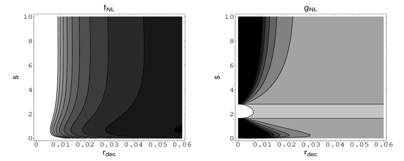
For the quartic case, $f_{\rm NL}$ does not show significant oscillatory features and consequently $n_{f_{\rm NL}}$ does not get enhanced for any value of the self-interaction strength parameter $s$. On the other hand, $g_{\rm NL}$ changes sign twice around $s\sim 2$, and in this region $n_{g_{\rm NL}}$ is considerably enhanced. The two divergent spikes seen in the plot for $n_{g_{\rm NL}}$ correspond to the points where $g_{\rm NL}=0$. When moving away from these points, $g_{\rm NL}$ starts to grow while $n_{g_{\rm NL}}$ still remains large. In the self-interaction dominated regime $s\gg 1$, both $n_{f_{\rm NL}}$ and $n_{g_{\rm NL}}$ asymptote to constant values. Indeed, in this limit equation (25) reduces to a simple power law $\sigma_{\rm osc}\propto\sigma(t_{k})^{3/4}$ which yields $f_{\rm NL}=10/(12r_{\rm dec})\,,~{}n_{f_{\rm NL}}=4\eta_{\sigma}$ and $g_{\rm NL}=-25/(54r_{\rm dec}^{2})\,,~{}n_{g_{\rm NL}}=-20\eta_{\sigma}$.

The quartic model nicely demonstrates how the interacting curvaton scenario can generate strongly scale-dependent non-Gaussianity. However, the results for $n_{g_{\rm NL}}$ are of limited observational interest because the bound $|f_{\rm NL}|\lesssim 10^{2}$ requires $g_{\rm NL}$ to be small $|g_{\rm NL}|\lesssim 10^{3}$, see Fig. 1. This is too small to be detectable with the CMB [51].

5 Non-renormalizable interactions

For non-renormalizable curvaton potentials, $n=6$ and $n=8$ in (3), we have used numerical methods similar to [26] to study the dynamics and compute the scale-dependence. In the interaction dominated regime, $s\gg 1$, it is also possible to obtain simple analytical estimates as we briefly discuss at the end of this section, see Sec. 5.1.

The presence of non-renormalizable self-interactions renders both $f_{\rm NL}$ and $g_{\rm NL}$ oscillatory functions of the self-interaction strength parameter $s$ [22]. The oscillatory behaviour can lead to great enhancement of the scale-dependence, as discussed above. This is clearly seen in Figure 3 which shows $|n_{f_{\rm NL}}|/\eta_{\sigma}$ and $|n_{g_{\rm NL}}|/\eta_{\sigma}$ as a function of $s$ for $n=6$. The results for $n=8$ are qualitatively similar.

Figure 3: Plot of $|n_{f_{\rm NL}}|/\eta_{\sigma}$ (red–solid line) and $|n_{g_{\rm NL}}|/\eta_{\sigma}$ (blue–dashed line) as a function of the self-interaction strength parameter $s$ for $n=6$.

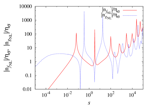
The spikes in the behaviour of $|n_{f_{\rm NL}}|$ in Figure 3 correspond to points where $f_{\rm NL}$ crosses zero. In the vicinity of these points $f_{\rm NL}$ takes non-zero, and for small $r_{\rm dec}$ observable, values while $|n_{f_{\rm NL}}|$ is one or two orders of magnitude enhanced compared to the slow–roll scale $\eta_{\sigma}$. Similar comments apply to $|n_{g_{\rm NL}}|$ whose behaviour is illustrated in the same figure.

In Figure 4 we compare our results with the predicted accuracy of Planck for observing the scale-dependence.

(a) $n=4$

(b) $n=6$

(c) $n=8$

(d) $n=6$

Figure 4: $f_{\rm NL}$ vs. $n_{f_{\rm NL}}$ for $n=4,6,8$ and $g_{\rm NL}$ vs. $n_{g_{\rm NL}}$ for $n=6$ with different choices of $r_{\rm dec}$ and $\eta_{\sigma}$. The points shown in the figures range from $s=10^{-5}$ to $s=10^{5}$. The black curves depict the forecasted observational sensitivity of Planck, the region of detectable $n_{f_{\rm NL}}$ lies outside the curves, i.e. further from the origin.

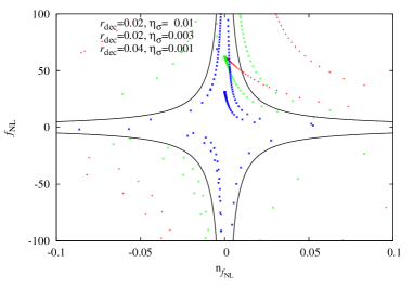
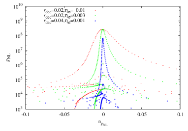
Figures 4(a), 4(b) and 4(c) show $f_{\rm NL}$ against $n_{f_{\rm NL}}$, scanning from $s=10^{-5}$ to $s=10^{5}$ and keeping $r_{\rm dec}$ and $\eta_{\sigma}$ fixed. Outside the black lines which denote $|n_{f_{\rm NL}}f_{\rm NL}=0.5|$, the scale-dependence is detectable by Planck at the $1$-$\sigma$ level (and at the $2$-$\sigma$ level with CMBPol) [13]. For $n=6$ and $n=8$, the points corresponding to a given choice of $r_{\rm dec}$ and $\eta_{\sigma}$ do not lie on a single curve as in the case $n=4$. This is again a manifestation of the oscillatory behaviour of $f_{\rm NL}$, characteristic for non-renormalizable self-interactions. However, it is noteworthy that it is possible to generate observable scale-dependence even for $n=4$, provided that the ratio $\eta_{\sigma}/r_{\rm dec}$ is large enough.

For comparison, we have also plotted $g_{\rm NL}$ against $n_{g_{\rm NL}}$ for $n=6$ in Figure 4(d). As $g_{\rm NL}$ and $n_{g_{\rm NL}}$ feel derivatives up to third order, this plot shows considerably more structure than the corresponding result for $f_{\rm NL}$ and $n_{f_{\rm NL}}$ (Figure 4(b)), which only feel derivatives up to second order. There are currently no forecasts on how well $n_{g_{\rm NL}}$ could be measured.

In Figure 5 we plot $n_{g_{\rm NL}}/n_{f_{\rm NL}}$ against $g_{\rm NL}/f_{\rm NL}^{2}$.

(a) $n=4$

(b) $n=6$

(c) $n=8$

Figure 5: The observables $g_{\rm NL}/f_{\rm NL}^{2}$ and $n_{g_{\rm NL}}/n_{f_{\rm NL}}$, which depend on the self-interaction strength $s$ only, plotted for $s=10^{-5}...10^{5}$. The points outside the curves are not accessible for any parameter values in the self-interacting curvaton scenario. In the case of a renormalisable self-interaction, $n=4$, we also plot points in green calculated using the analytic formula.

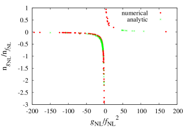
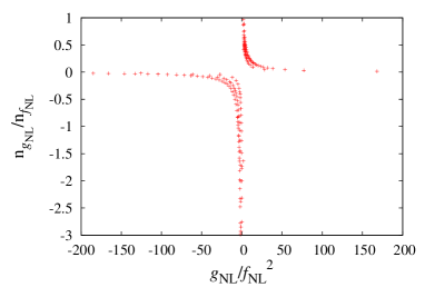
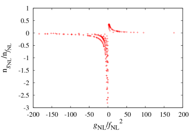
These ratios only depend on the self-interaction strength parameter $s$. The points depicted in the figure range from $s=10^{-5}$ to $s=10^{5}$. The predictions asymptote to constant values both for $s\rightarrow 0$ and $s\rightarrow\infty$ and extending the plot region to smaller or larger $s$-values essentially leaves the plots unchanged. Therefore, only the points that lie on the curves seen in Figure 5 are accessible in the self-interacting curvaton scenario. The region outside the curves can not be accessed for any parameter values. Despite its very rich structure and broad range of different observational imprints [22, 26], the self-interacting curvaton scenario could therefore be ruled out by a combined detection of $f_{\rm NL}$ and $g_{\rm NL}$ and their scale-dependencies.

5.1 Interaction dominated regime

In the interaction dominated regime $s\gg 1$, it is possible to derive analytical results even for the non-renormalizable case. In this regime the curvaton oscillations start in the non-renormalizable part of the potential and the transition to the quadratic potential takes place relatively late after the onset of oscillations. The dynamics can therefore be described by the simple scaling law $\rho_{\sigma}\propto a^{-6n/(n+2)}$, unlike for smaller values of $s$ [26]. For $s\gg 1$, the transition time can be estimated by $\lambda\sigma^{n-2}\sim m^{2}$ which yields ${\sigma}_{{\rm osc}}\propto\sigma(t_{k})s^{-1/8}(1+{\cal O}(\eta_{\sigma}))$. Using this in equations (14) – (3) we obtain the results

$$f_{\rm NL} = \frac{1}{r_{\rm dec}}\frac{5(6-n)}{2(10-n)}+{\cal O}\left(\frac{\eta_{\sigma}}{r_{\rm dec}}\right)\ ,\;\;n_{f_{\rm NL}}f_{\rm NL}=\frac{\eta_{\sigma}}{r_{\rm dec}}\frac{10(n-2)}{10-n}+{\cal O}\left(\frac{\epsilon^{2}}{r_{\rm dec}}\right)\ ,$$ (26)

$$g_{\rm NL} = f_{\rm NL}^{2}\frac{2(2-n)}{3(6-n)}+{\cal O}\left(\frac{\eta_{\sigma}}{r_{\rm dec}^{2}}\right)\ ,\;\;n_{g_{\rm NL}}g_{\rm NL}=\frac{\eta_{\sigma}}{r_{\rm dec}^{2}}\frac{50(6+n)}{3(10-n)}+{\cal O}\left(\frac{\epsilon^{2}}{r_{\rm dec}}\right)\ .$$ (27)

The results for $n=4$ agree with the discussion in Section 4. For $n=6$, the amplitudes $f_{\rm NL}$ and $g_{\rm NL}$ vanish to leading order in slow roll, $f_{\rm NL}={\cal O}(\eta_{\sigma}/r_{\rm dec})$, $g_{\rm NL}=(\eta_{\sigma}/r_{\rm dec}^{2})$, and we find $n_{f_{\rm NL}}={\cal O}(1),n_{g_{\rm NL}}={\cal O}(1)$. The first order slow roll computation used in our analysis is not enough to derive explicit results for this case but the level of non-Gaussianity is clearly unobservably small. For $n=8$ we find $f_{\rm NL}=-5/(2r_{\rm dec})$, $g_{\rm NL}=2f_{\rm NL}^{2}$, $n_{f_{\rm NL}}=-12\eta_{\sigma}$ and $n_{g_{\rm NL}}=28\eta_{\sigma}$. We have checked that these analytical estimates agree with our numerical simulations.

We note that our results do not agree with those in [29], in particular compare with Eq. (2.56) of [29] in the large $s$ limit, where the sign of $g_{\rm NL}$ was found to be positive for all values of $n$. We do not attempt to explain the difference, but we note again that we have found a good agreement between our analytic and numerical results, both here for the interaction dominated regime as well as for the $n=4$ case, see for example Fig. 5(a).

6 Conclusions

We have studied the scale-dependence of the non-linearity parameters, especially of $f_{\rm NL}$ and $g_{\rm NL}$ in the curvaton scenario allowing for the possibility of a large self interaction. We have found a rich structure in the results, and that a much larger scale dependence of the non-linearity parameters is possible than may be expected by comparison to the observed spectral index of the power spectrum. This boosts the observational prospects for detecting non-Gaussianity and its scale-dependence and shows that Planck may achieve a simultaneous detection of $f_{\rm NL}$ and $n_{f_{\rm NL}}$. This would put stringent constraints on the curvaton scenario and rule out its simplest and most studied version, the curvaton with a quadratic potential.

Although the richness of the results, as shown in the many plots, makes it hard to make firm predictions of the curvaton scenario, one can observe some interesting general trends in the results. In general, increasing the strength of the self interaction $s$, and/or the power of the self-coupling $n$ leads to larger values of the scale-dependence as well as an oscillatory structure. Due to their dependence on a third derivative, $g_{\rm NL}$ and $n_{g_{\rm NL}}$ have a more complex structure than $f_{\rm NL}$ and $n_{f_{\rm NL}}$, which only depend on a second derivative. In the limit of no self-interaction, i.e. $s=0$, we recover a constant and potentially large $f_{\rm NL}$. However $g_{\rm NL}\simeq 0$ is far too small to be observable in this limit.

Previous studies of scale-dependence in non-quadratic curvaton scenario’s had focussed on a region with only small self-interactions. In that regime and for the models studied in this article it was found that $n_{f_{\rm NL}}>0$ [21], while for an axionic curvaton potential the opposite sign was found [52]. In both cases the sign of $n_{f_{\rm NL}}$ was given by the sign of the third derivative of the potential. However we have here shown that even for a fixed potential the sign of $n_{f_{\rm NL}}$ may oscillate, depending on the initial field value, which affects the self–interaction strength $s$. For a quartic self–interaction there are only oscillations in the sign of $n_{g_{\rm NL}}$ but not $n_{f_{\rm NL}}$, for higher powers of the self interaction multiple oscillations in both of these parameters occurs.

The scale dependence of the non–linearity parameters does linearily depend on the $\eta_{\sigma}$ slow-roll parameter, just as the power spectrum’s spectral index does (provided that the $\epsilon$ slow-roll parameter is subdominant, one has $n_{s}-1=2\eta_{\sigma}$). However the numerical coefficient in the case of $n_{f_{\rm NL}}$ and $n_{g_{\rm NL}}$ also depends on the value of the self–interaction strength and can become very large in cases where the amplitude of the non-linearity parameters become supressed, but they may still remain observable provided that the curvaton is sufficiently subdominant at the time of decay. In the limit of a large self–interaction strength with an octic self interaction, which does not correspond to any suppression of the non-linearity parameters we find $n_{f_{\rm NL}}\simeq-12\eta_{\sigma}$ and $n_{g_{\rm NL}}\simeq 28\eta_{\sigma}$, both of which are an order of magnitude larger than the spectral index.

This rich structure of the self–interacting curvaton does not make the model unpredictive or unfalsifiable, there are model constraints, for example on how late the curvaton decays and on the observed amplitude of the power spectrum which restrict the allowed model parameters. The fact that the model can be observationally ruled out is clear from the plots relating $f_{\rm NL},g_{\rm NL},n_{f_{\rm NL}}$ and $n_{g_{\rm NL}}$ given in Fig. 5, only a few lines in parameter space are allowed.

Appendix A On the accuracy of the results

In computing the scale-dependence, we have neglected the non-Gaussianities of the curvaton perturbations $\delta\sigma_{{\bf k}}(t_{k})$ at horizon crossing, following [10, 11]. Since we assume canonical slow-roll dynamics for the curvaton during inflation, the neglected parts are in general slow-roll suppressed. (For a discussion of the scale-dependence of the three and four-point functions of a test field $\delta\sigma_{{\bf k}}(t_{k})$, see [53].) These non-Gaussianities can however play a key role if $|n_{f_{\rm NL}}|$ or $|n_{g_{\rm NL}}|$ become of order unity.

In this Appendix we address this issue by considering a (unrealistic) toy model with a quartic curvaton

$$V(\sigma)=\lambda\sigma^{4}\ ,$$ (28)

and a vanishing classical background field $\sigma=0$. The inflationary stage is described by a de Sitter solution. While this model cannot lead to a successful curvaton scenario, it clearly demonstrates how the non-Gaussianities of $\delta\sigma_{{\bf k}}(t_{k})$ can become important.

The connected four-point function of the massless curvaton fluctuations, evaluated at some time $t_{i}$ after the horizon exit of all the four modes, can be written as [54, 55, 53]

$$\langle\delta\sigma_{{\bf k}_{1}}(t_{i})\delta\sigma_{{\bf k}_{2}}(t_{i})\delta\sigma_{{\bf k}_{3}}(t_{i})\delta\sigma_{{\bf k}_{4}}(t_{i})\rangle = (2\pi)^{3}\delta(\sum{\bf k}_{m})\frac{8\lambda}{H^{2}}\left(\gamma+\xi(\{k_{m}\})+{\rm ln}\frac{\sum k_{m}}{k_{i}}\right)\times$$ (29)

$$\left(P(k_{1})P(k_{2})P(k_{3})+{\rm perm.}\right)+{\cal O}(\lambda^{2})\ .$$

Here $\gamma\simeq 0.58$ is the Euler-Mascheroni constant and $\xi(\{k_{m}\})$ is a dimensionless function of the all the four wavenumbers $k_{m}$, see [53] for details. $P(k)$ is the spectrum of curvaton fluctuations and $k_{i}$ is the mode crossing the horizon at $t_{i}$. To first order in the coupling $\lambda$, there are no other connected $n$-point functions $(n>2)$.

The four–point function affects the trispectrum of curvature perturbation. Using the $\delta N$ formalism together with (29), we find the non-linearity parameter $g_{\rm NL}$ given by

$$g_{\rm NL}=\frac{25}{54}\frac{N^{\prime\prime\prime}}{N^{\prime 3}}\left(1+n^{0}_{g_{\rm NL}}\left(\gamma+\xi({k_{m}})+{\rm ln}\frac{\sum k_{m}}{k_{i}}\right)\right)\ .$$ (30)

Here $n^{0}_{g_{\rm NL}}$ denotes the scale-dependence given by (3),

$$n^{0}_{g_{\rm NL}}=\frac{N^{\prime}}{N^{\prime\prime\prime}}\frac{V^{\prime\prime\prime\prime}}{3H^{2}}\ ,$$ (31)

computed assuming the modes $\delta\sigma_{{\bf k}}(t_{k})$ are Gaussian. (The part proportional to $n_{f_{\rm NL}}$ in (3) vanishes as $V^{\prime\prime\prime}(0)=0$ here.)

Concentrating, for simplicity, on equilateral configurations $k_{m}=k$, and setting $t_{i}=t_{k}$, we obtain

$$g_{\rm NL} = \frac{25}{54}\frac{N^{\prime\prime\prime}}{N^{\prime 3}}\left(1+n^{0}_{g_{\rm NL}}(\gamma-\frac{51}{16}+{\rm ln}\,4)\right)\ ,$$ (32)

$$n_{g_{\rm NL}} = \frac{n^{0}_{g_{\rm NL}}}{1+n^{0}_{g_{\rm NL}}(\gamma-\frac{51}{16}+{\rm ln}\,4)}\ .$$ (33)

The term $n^{0}_{g_{\rm NL}}(\gamma-51/16+{\rm ln}\,4)\simeq-1.2\,n^{0}_{g_{\rm NL}}$ in (32) and (33) arises from the connected four-point function (29) of curvaton fluctuations, that is from the non-Gaussianity of $\delta\sigma_{{\bf k}}(t_{k})$. For $|n^{0}_{g_{\rm NL}}|\ll 1$, these corrections can be neglected and we recover the results previously used in this work. However, if $|n^{0}_{g_{\rm NL}}|\gtrsim 1$ the corrections clearly have a significant effect on both the amplitude $g_{\rm NL}$ and its scale-dependence.

It is straightforward to see that the results get modified in a qualitatively similar manner for models with realistic potential and a non-vanishing background field $\sigma$,

$$f_{\rm NL} = \frac{5}{6}\frac{N^{\prime\prime}}{N^{\prime 2}}\left(1+{\cal O}(n^{0}_{f_{\rm NL}})\right)\ ,\qquad n_{f_{\rm NL}}=\frac{n^{0}_{f_{\rm NL}}}{1+{\cal O}(n^{0}_{f_{\rm NL}})}\ ,$$ (34)

$$g_{\rm NL} = \frac{25}{54}\frac{N^{\prime\prime\prime}}{N^{\prime 3}}\left(1+{\cal O}(n^{0}_{g_{\rm NL}})\right)\ ,\qquad n_{g_{\rm NL}}=\frac{n^{0}_{g_{\rm NL}}}{1+{\cal O}(n^{0}_{g_{\rm NL}})}\ .$$ (35)

Therefore, we conclude quite generally that non-Gaussianities of the curvaton perturbations can be safely neglected if $|n^{0}_{f_{\rm NL}}|\ll 1$ and $|n^{0}_{g_{\rm NL}}|\ll 1$. However, if $n^{0}_{f_{\rm NL}}$ or $n^{0}_{g_{\rm NL}}$ become large a more careful analysis is needed, not only to compute the scale-dependence but also to find the correct results for $f_{\rm NL}$ and $g_{\rm NL}$.

References

- [1] M. Liguori, E. Sefusatti, J. R. Fergusson, E. P. S. Shellard, Adv. Astron. 2010, 980523 (2010). [arXiv:1001.4707 [astro-ph.CO]].
- [2] X. Chen, Adv. Astron. 2010, 638979 (2010). [arXiv:1002.1416 [astro-ph.CO]].
- [3] C. T. Byrnes, K. -Y. Choi, Adv. Astron. 2010, 724525 (2010). [arXiv:1002.3110 [astro-ph.CO]].
- [4] E. Komatsu, Class. Quant. Grav. 27, 124010 (2010). [arXiv:1003.6097 [astro-ph.CO]].
- [5] D. Wands, Class. Quant. Grav. 27, 124002 (2010). [arXiv:1004.0818 [astro-ph.CO]].
- [6] G. Dvali, A. Gruzinov and M. Zaldarriaga, Phys. Rev. D 69, 023505 (2004) [arXiv:astro-ph/0303591].
- [7] L. Kofman, arXiv:astro-ph/0303614.
- [8] K. Enqvist and M. S. Sloth, Nucl. Phys. B 626, 395 (2002) [arXiv:hep-ph/0109214]; D. H. Lyth and D. Wands, Phys. Lett. B 524, 5 (2002) [arXiv:hep-ph/0110002]; T. Moroi and T. Takahashi, Phys. Lett. B 522, 215 (2001) [Erratum-ibid. B 539, 303 (2002)] [arXiv:hep-ph/0110096]; A. D. Linde and V. F. Mukhanov, Phys. Rev. D 56 (1997) 535 [arXiv:astro-ph/9610219]; S. Mollerach, Phys. Rev. D 42 (1990) 313.
- [9] D. H. Lyth, C. Ungarelli and D. Wands, Phys. Rev. D 67, 023503 (2003) [arXiv:astro-ph/0208055].
- [10] C. T. Byrnes, S. Nurmi, G. Tasinato and D. Wands, JCAP 1002 (2010) 034 [arXiv:0911.2780 [astro-ph.CO]].
- [11] C. T. Byrnes, M. Gerstenlauer, S. Nurmi, G. Tasinato and D. Wands, JCAP 1010 (2010) 004 [arXiv:1007.4277 [astro-ph.CO]].
- [12] M. LoVerde, A. Miller, S. Shandera, L. Verde, JCAP 0804, 014 (2008). [arXiv:0711.4126 [astro-ph]].
- [13] E. Sefusatti, M. Liguori, A. P. S. Yadav, M. G. Jackson and E. Pajer, JCAP 0912 (2009) 022 [arXiv:0906.0232 [astro-ph.CO]].
- [14] S. Shandera, N. Dalal, D. Huterer, JCAP 1103, 017 (2011). [arXiv:1010.3722 [astro-ph.CO]].
- [15] A. Becker, D. Huterer, K. Kadota, JCAP 1101, 006 (2011). [arXiv:1009.4189 [astro-ph.CO]].
- [16] A. Riotto, M. S. Sloth, Phys. Rev. D83, 041301 (2011). [arXiv:1009.3020 [astro-ph.CO]].
- [17] X. Chen, Phys. Rev. D72, 123518 (2005). [astro-ph/0507053].
- [18] N. Bartolo, M. Fasiello, S. Matarrese, A. Riotto, JCAP 1012, 026 (2010). [arXiv:1010.3993 [astro-ph.CO]].
- [19] J. Noller, J. Magueijo, Phys. Rev. D83, 103511 (2011). [arXiv:1102.0275 [astro-ph.CO]].
- [20] C. Burrage, R. H. Ribeiro, D. Seery, JCAP 1107, 032 (2011). [arXiv:1103.4126 [astro-ph.CO]].
- [21] C. T. Byrnes, K. Enqvist and T. Takahashi, JCAP 1009 (2010) 026 [arXiv:1007.5148 [astro-ph.CO]].
- [22] K. Enqvist, S. Nurmi, O. Taanila and T. Takahashi, JCAP 1004 (2010) 009 [arXiv:0912.4657 [astro-ph.CO]].
- [23] M. Kawasaki, T. Kobayashi and F. Takahashi, arXiv:1107.6011 [astro-ph.CO].
- [24] K. Enqvist, S. Nurmi, JCAP 0510, 013 (2005). [astro-ph/0508573].
- [25] K. Enqvist and T. Takahashi, JCAP 0809 (2008) 012 [arXiv:0807.3069 [astro-ph]].
- [26] K. Enqvist, S. Nurmi, G. Rigopoulos, O. Taanila and T. Takahashi, JCAP 0911 (2009) 003 [arXiv:0906.3126 [astro-ph.CO]].
- [27] K. -Y. Choi, O. Seto, Phys. Rev. D82, 103519 (2010). [arXiv:1008.0079 [astro-ph.CO]].
- [28] J. Fonseca, D. Wands, Phys. Rev. D83, 064025 (2011). [arXiv:1101.1254 [astro-ph.CO]].
- [29] Q. -G. Huang, JCAP 0811, 005 (2008). [arXiv:0808.1793 [hep-th]].
- [30] K. Dimopoulos, G. Lazarides, D. Lyth and R. Ruiz de Austri, Phys. Rev. D 68 (2003) 123515 [arXiv:hep-ph/0308015].
- [31] M. Kawasaki, K. Nakayama and F. Takahashi, JCAP 0901 (2009) 026 [arXiv:0810.1585 [hep-ph]].
- [32] P. Chingangbam and Q. G. Huang, JCAP 0904 (2009) 031 [arXiv:0902.2619 [astro-ph.CO]].
- [33] D. Langlois and F. Vernizzi, Phys. Rev. D 70 (2004) 063522 [arXiv:astro-ph/0403258]; G. Lazarides, R. R. de Austri and R. Trotta, Phys. Rev. D 70 (2004) 123527 [arXiv:hep-ph/0409335]; F. Ferrer, S. Rasanen and J. Valiviita, JCAP 0410 (2004) 010 [arXiv:astro-ph/0407300]; T. Moroi, T. Takahashi and Y. Toyoda, Phys. Rev. D 72, 023502 (2005) [arXiv:hep-ph/0501007]; T. Moroi and T. Takahashi, Phys. Rev. D 72, 023505 (2005) [arXiv:astro-ph/0505339]; K. Ichikawa, T. Suyama, T. Takahashi and M. Yamaguchi, Phys. Rev. D 78, 023513 (2008) [arXiv:0802.4138 [astro-ph]]; D. Langlois, F. Vernizzi and D. Wands, JCAP 0812 (2008) 004 [arXiv:0809.4646 [astro-ph]].
- [34] K. A. Malik, D. H. Lyth, JCAP 0609, 008 (2006). [astro-ph/0604387].
- [35] M. Sasaki, J. Valiviita, D. Wands, Phys. Rev. D74, 103003 (2006). [astro-ph/0607627].
- [36] K. Enqvist, S. Nurmi, G. I. Rigopoulos, JCAP 0810, 013 (2008). [arXiv:0807.0382 [astro-ph]].
- [37] A. Chambers, S. Nurmi and A. Rajantie, JCAP 1001 (2010) 012 [arXiv:0909.4535 [astro-ph.CO]].
- [38] A. A. Starobinsky, JETP Lett. 42, 152 (1985) [Pisma Zh. Eksp. Teor. Fiz. 42, 124 (1985)].
- [39] M. Sasaki and E. D. Stewart, Prog. Theor. Phys. 95 (1996) 71 [arXiv:astro-ph/9507001].
- [40] M. Sasaki and T. Tanaka, Prog. Theor. Phys. 99, 763 (1998) [arXiv:gr-qc/9801017].
- [41] D. H. Lyth, K. A. Malik and M. Sasaki, JCAP 0505, 004 (2005) [arXiv:astro-ph/0411220].
- [42] D. H. Lyth and Y. Rodriguez, Phys. Rev. Lett. 95 (2005) 121302 [arXiv:astro-ph/0504045].
- [43] T. Suyama, T. Takahashi, M. Yamaguchi, S. Yokoyama, JCAP 1012, 030 (2010). [arXiv:1009.1979 [astro-ph.CO]].
- [44] Q. G. Huang, JCAP 1104 (2011) 010 [arXiv:1102.4686 [astro-ph.CO]].
- [45] E. Komatsu et al. [ WMAP Collaboration ], Astrophys. J. Suppl. 192, 18 (2011). [arXiv:1001.4538 [astro-ph.CO]].
- [46] L. Alabidi, K. Malik, C. T. Byrnes, K. -Y. Choi, JCAP 1011, 037 (2010). [arXiv:1002.1700 [astro-ph.CO]].
- [47] J. Kumar, L. Leblond and A. Rajaraman, JCAP 1004 (2010) 024 [arXiv:0909.2040 [astro-ph.CO]].
- [48] T. Suyama, F. Takahashi, JCAP 0809, 007 (2008). [arXiv:0804.0425 [astro-ph]].
- [49] J. Bramante, J. Kumar, [arXiv:1107.5362 [astro-ph.CO]].
- [50] D. Seery, Class. Quant. Grav. 27, 124005 (2010). [arXiv:1005.1649 [astro-ph.CO]].
- [51] J. Smidt, A. Amblard, C. T. Byrnes, A. Cooray, A. Heavens, D. Munshi, Phys. Rev. D81, 123007 (2010). [arXiv:1004.1409 [astro-ph.CO]].
- [52] Q. -G. Huang, JCAP 1011, 026 (2010). [arXiv:1008.2641 [astro-ph.CO]].
- [53] F. Bernardeau, JCAP 1102 (2011) 017 [arXiv:1003.3575 [astro-ph.CO]].
- [54] M. Zaldarriaga, Phys. Rev. D 69 (2004) 043508 [arXiv:astro-ph/0306006].
- [55] F. Bernardeau, T. Brunier and J. P. Uzan, Phys. Rev. D 69 (2004) 063520 [arXiv:astro-ph/0311422].