Natures of Statefinder Parameters and Om Diagnostic for Cardassian Universe in Horˇˇr\check{\text{r}}ava-Lifshitz Gravity

Piyali Bagchi Khatua1111piyali.bagchi@yahoo.co.in and Ujjal Debnath2222ujjaldebnath@yahoo.com 1Department of Computer Sc and Engg, Netaji Subhas Engineering College, Garia, Kolkata-700 152, India.
2Department of Mathematics, Bengal Engineering and Science University, Shibpur, Howrah-711 103, India.
Abstract

In this work, we have considered Cardassian Universe in Horˇˇr\check{\text{r}}ava-Lifshitz gravity. Four types of Cardassian Universe models i.e., polytropic/power law, modified polytropic, exponential and modified exponential models have been considered for accelerating models. The natures of statefinder parameters, deceleration parameter, Om𝑂𝑚Om diagnostic and EoS parameters have been investigated for all types of Cardassian models in Horˇˇr\check{\text{r}}ava-Lifshitz gravity.

I Introduction

Recent observations of the luminosity of type Ia supernovae indicate an accelerated expansion of the universe [1-7] and lead to the search for a new type of matter, called dark energy, which violates the strong energy condition [8-10]. For explaining the accelerating expansion of the universe, large number of cosmological models have been proposed. Dark energy model is proposed by assuming an energy component with negative pressure in the universe, this dark energy dominates the total energy density of the universe and drives its acceleration of expansion at recent times. Some authors have explored possible explanations for the acceleration: (i) cosmological constant, (ii) quintessence [11-17], (iii) gravitational leakage into extra dimensions [18-19]. Accelerated expansion also depends on other observations such as the cosmic microwave background (CMB) [20] and galaxy power spectra [21]. Another reason of acceleration is the geometric effect of the general relativity fails in the present cosmic time space scale. The model proposed by Freese and Lewisan, called Cardassian model [22-26], assume that the universe is flat and accelerating which consists only of matter and radiation [27]. The geometry is flat as required by measurements of the cosmic background radiation, so that there are no curvature terms in the equation and no vacuum term in the equation and so the model does not address the cosmological constant. In Cardassian Model, we take g(ρ)𝑔𝜌g(\rho) as a function of ρ𝜌\rho that returns simply to l2ρ/3superscript𝑙2𝜌3l^{2}\rho/3 at early epochs, where l2=8πGcsuperscript𝑙28𝜋subscript𝐺𝑐l^{2}=8\pi G_{c}.

On the basis of the recent observation one can state that if Einstein’s theory of gravity is acceptable on cosmological scales, then our universe must dominated by a mysterious form of energy called dark energy. Recently Horˇˇr\check{\text{r}}ava [28-29] proposed a new theory of gravity, which renormalizable with higher spatial derivatives in four dimensions which reduces to Einstein’s gravity with non vanishing cosmological constant in IR but with improved UV behaviours. In Lifshitz [30] scalar field theory the time dimension has weight 3 if a space dimension has weight 1 and this theory is called Horˇˇr\check{\text{r}}ava-Lifshitz gravitational theory. Horˇˇr\check{\text{r}}ava-Lifshitz gravity has been studied and extended in detail and applied as a cosmological framework of the universe [31-33].

As so many cosmological models have been developed, so for discrimination between these contenders, Sahni et al [34] proposed a new geometrical diagnostic named the statefinder pair {r,s}𝑟𝑠\{r,s\}, where r𝑟r is generated from the scalar factor a𝑎a and its derivatives with respect to the cosmic time t𝑡t and s𝑠s is a simple combination of r𝑟r and the deceleration parameter q𝑞q. Clear differences for the evolutionary trajectories in the r𝑟r-s𝑠s plane have been found. In this work, we have discussed four different types of Cardassian Universe models in Horˇˇr\check{\text{r}}ava-Lifshitz gravity. In every case we find the statefinder parameters, deceleration parameter and Om𝑂𝑚Om diagnostic [34-36].

II Cardassian Universe in Horˇˇr\check{\text{r}}ava-Lifshitz Gravity

The Arnowitt-Deser-Misner formalism of the full metric is written as [37],

ds2=N2dt2+gij(dxi+Nidt)(dxj+Njdt)𝑑superscript𝑠2superscript𝑁2𝑑superscript𝑡2subscript𝑔𝑖𝑗𝑑superscript𝑥𝑖superscript𝑁𝑖𝑑𝑡𝑑superscript𝑥𝑗superscript𝑁𝑗𝑑𝑡ds^{2}=-N^{2}dt^{2}+g_{ij}(dx^{i}+N^{i}dt)(dx^{j}+N^{j}dt) (1)

Under the detailed balance condition the full action condition of Horˇˇr\check{\text{r}}ava-Lifshitz gravity is given by,

S=dtd3xgN[2κ2(KijKijλK2)+κ22ω4CijCijκ2μϵijk2ω2gRiljRkl\displaystyle S=\int dtd^{3}x\sqrt{g}N\left[\frac{2}{\kappa^{2}}(K_{ij}K^{ij}-\lambda K^{2})+\frac{\kappa^{2}}{2\omega^{4}}C_{ij}C^{ij}-\frac{\kappa^{2}\mu\epsilon^{ijk}}{2\omega^{2}\sqrt{g}}R_{il}\nabla_{j}R^{l}_{k}\right.
+κ2μ28RijRij+κ2μ28(3λ1)(14λ4R2+ΛR3Λ2)]\left.+\frac{\kappa^{2}\mu^{2}}{8}R_{ij}R^{ij}+\frac{\kappa^{2}\mu^{2}}{8(3\lambda-1)}\left(\frac{1-4\lambda}{4}R^{2}+\Lambda R-3\Lambda^{2}\right)\right] (2)

where the extrinsic curvature and Cotton tensor is defined as, Kij=12N(g˙ijiNjjNi)andCij=ϵiklgk(Rij14Rδlj)formulae-sequencesubscript𝐾𝑖𝑗12𝑁subscript˙𝑔𝑖𝑗subscript𝑖subscript𝑁𝑗subscript𝑗subscript𝑁𝑖𝑎𝑛𝑑superscript𝐶𝑖𝑗superscriptitalic-ϵ𝑖𝑘𝑙𝑔subscript𝑘subscriptsuperscript𝑅𝑗𝑖14𝑅subscriptsuperscript𝛿𝑗𝑙K_{ij}=\frac{1}{2N}(\dot{g}_{ij}-\nabla_{i}N_{j}-\nabla_{j}N_{i})~{}~{}~{}and~{}~{}~{}~{}~{}~{}C^{ij}=\frac{\epsilon^{ikl}}{\sqrt{g}}\nabla_{k}(R^{j}_{i}-\frac{1}{4}R\delta^{j}_{l}). The covariant derivatives are defined w.r.t. the spatial metric gijsubscript𝑔𝑖𝑗g_{ij}. ϵijksuperscriptitalic-ϵ𝑖𝑗𝑘\epsilon^{ijk} is the totally antisymmetric unit tensor, λ𝜆\lambda is a dimensionless coupling constant and the variable κ𝜅\kappa , ω𝜔\omega and μ𝜇\mu are constants with mass dimensions 1,0,1101-1,~{}0,~{}1 respectively. Also ΛΛ\Lambda is a positive constant, which as usual is related to the cosmological constant in the IR limit.

Now, in order to focus on cosmological frameworks, we impose the so called projectability condition and use a Friedmann-Robertson-Walker (FRW) metric we get, N=1,gij=a2(t)γij,Ni=0formulae-sequence𝑁1formulae-sequencesubscript𝑔𝑖𝑗superscript𝑎2𝑡subscript𝛾𝑖𝑗superscript𝑁𝑖0N=1,g_{ij}=a^{2}(t)\gamma_{ij},N^{i}=0 with γijdxidxj=dr21kr2+r2dΩ22subscript𝛾𝑖𝑗𝑑superscript𝑥𝑖𝑑superscript𝑥𝑗𝑑superscript𝑟21𝑘superscript𝑟2superscript𝑟2𝑑subscriptsuperscriptΩ22\gamma_{ij}dx^{i}dx^{j}=\frac{dr^{2}}{1-kr^{2}}+r^{2}d\Omega^{2}_{2} where k=0,1,+1𝑘011k=0,-1,+1 corresponding to flat, open and closed respectively. By varying N𝑁N and gijsubscript𝑔𝑖𝑗g_{ij}, we obtain the non-vanishing equations of motions:

H2=κ26(3λ1)ρ+κ26(3λ1)[3κ2μ2k28(3λ1)a4+3κ2μ2Λ28(3λ1)]κ4μ2kΛ8(3λ1)2a2superscript𝐻2superscript𝜅263𝜆1𝜌superscript𝜅263𝜆1delimited-[]3superscript𝜅2superscript𝜇2superscript𝑘283𝜆1superscript𝑎43superscript𝜅2superscript𝜇2superscriptΛ283𝜆1superscript𝜅4superscript𝜇2𝑘Λ8superscript3𝜆12superscript𝑎2H^{2}=\frac{\kappa^{2}}{6(3\lambda-1)}~{}\rho+\frac{\kappa^{2}}{6(3\lambda-1)}\left[\frac{3\kappa^{2}\mu^{2}k^{2}}{8(3\lambda-1)a^{4}}+\frac{3\kappa^{2}\mu^{2}\Lambda^{2}}{8(3\lambda-1)}\right]-\frac{\kappa^{4}\mu^{2}k\Lambda}{8(3\lambda-1)^{2}a^{2}} (3)

and

H˙+32H2=κ24(3λ1)pκ24(3λ1)[κ2μ2k28(3λ1)a43κ2μ2Λ28(3λ1)]κ4μ2kΛ16(3λ1)2a2˙𝐻32superscript𝐻2superscript𝜅243𝜆1𝑝superscript𝜅243𝜆1delimited-[]superscript𝜅2superscript𝜇2superscript𝑘283𝜆1superscript𝑎43superscript𝜅2superscript𝜇2superscriptΛ283𝜆1superscript𝜅4superscript𝜇2𝑘Λ16superscript3𝜆12superscript𝑎2\dot{H}+\frac{3}{2}H^{2}=-\frac{\kappa^{2}}{4(3\lambda-1)}~{}p-\frac{\kappa^{2}}{4(3\lambda-1)}\left[\frac{\kappa^{2}\mu^{2}k^{2}}{8(3\lambda-1)a^{4}}-\frac{3\kappa^{2}\mu^{2}\Lambda^{2}}{8(3\lambda-1)}\right]-\frac{\kappa^{4}\mu^{2}k\Lambda}{16(3\lambda-1)^{2}a^{2}} (4)

where Ha˙a𝐻˙𝑎𝑎H\equiv\frac{\dot{a}}{a} is the Hubble parameter. Here Gcsubscript𝐺𝑐G_{c} and G𝐺G is defined as, Gc=κ216π(3λ1)subscript𝐺𝑐superscript𝜅216𝜋3𝜆1G_{c}=\frac{\kappa^{2}}{16\pi(3\lambda-1)} and G=κ232π𝐺superscript𝜅232𝜋G=\frac{\kappa^{2}}{32\pi} where Gcsubscript𝐺𝑐G_{c} is the “cosmological” Newton’s constant and G𝐺G is the “gravitational” Newton’s constant.

We can re-write the above equations as [38],

H2+ka2=l2ρ3+k22Λa4+Λ2superscript𝐻2𝑘superscript𝑎2superscript𝑙2𝜌3superscript𝑘22Λsuperscript𝑎4Λ2H^{2}+\frac{k}{a^{2}}=\frac{l^{2}\rho}{3}+\frac{k^{2}}{2\Lambda a^{4}}+\frac{\Lambda}{2} (5)

and

H˙+32H2+k2a2=l2p2k24Λa4+3Λ4˙𝐻32superscript𝐻2𝑘2superscript𝑎2superscript𝑙2𝑝2superscript𝑘24Λsuperscript𝑎43Λ4\dot{H}+\frac{3}{2}H^{2}+\frac{k}{2a^{2}}=-\frac{l^{2}p}{2}-\frac{k^{2}}{4\Lambda a^{4}}+\frac{3\Lambda}{4} (6)

Here, ρ𝜌\rho and p𝑝p are respectively the energy density and pressure of the universe, l2=8πGcsuperscript𝑙28𝜋subscript𝐺𝑐l^{2}=8\pi G_{c} and choosing 8πG=18𝜋𝐺18\pi G=1.

Freese and Lewis [22] constructed Cardassian universe models so that, in Cardassian models the universe is flat and accelerating, and yet contains only matter (baryonic or not) and radiation. The above equation governing the expansion of the universe is modified to,

H2+ka2=l2g(ρ)3+k22Λa4+Λ2superscript𝐻2𝑘superscript𝑎2superscript𝑙2𝑔𝜌3superscript𝑘22Λsuperscript𝑎4Λ2H^{2}+\frac{k}{a^{2}}=\frac{l^{2}g(\rho)}{3}+\frac{k^{2}}{2\Lambda a^{4}}+\frac{\Lambda}{2} (7)

which gives,

H=ka2+l2g(ρ)3+k22Λa4+Λ2𝐻𝑘superscript𝑎2superscript𝑙2𝑔𝜌3superscript𝑘22Λsuperscript𝑎4Λ2H=\sqrt{-\frac{k}{a^{2}}+\frac{l^{2}g(\rho)}{3}+\frac{k^{2}}{2\Lambda a^{4}}+\frac{\Lambda}{2}} (8)

where ρ𝜌\rho is the total energy density of matter and radiation and we will neglect the contribution of radiation for the late-time evolution of the universe. The function g(ρ)𝑔𝜌g(\rho) reduces to ρ𝜌\rho in the early universe. Now,

g(ρ)=ρm+ρcandp=pm+pcformulae-sequence𝑔𝜌subscript𝜌𝑚subscript𝜌𝑐𝑎𝑛𝑑𝑝subscript𝑝𝑚subscript𝑝𝑐g(\rho)=\rho_{m}+\rho_{c}~{}~{}~{}~{}and~{}~{}~{}~{}~{}~{}p=p_{m}+p_{c} (9)

where ρmsubscript𝜌𝑚\rho_{m} and ρcsubscript𝜌𝑐\rho_{c} are the energy densities of matter and Cardassian term of the universe respectively and pmsubscript𝑝𝑚p_{m} and pcsubscript𝑝𝑐p_{c} are the pressure of matter and Cardassian term of the universe respectively. For any suitable Cardassian model, the following requirements that should be fulfilled. (i) The function g(ρ)𝑔𝜌g(\rho) should returns to the usual form of ρ𝜌\rho at early epochs in order to recover the thermal history of the standard cosmological. (ii) g(ρ)𝑔𝜌g(\rho) should takes a different form at late times when zO(1)𝑧O1z\thicksim\textrm{O}(1) in order to drive an accelerated expansion as indicated by the observation of SNeIa. (iii) The classical solution of the expansion should be stable, and the sound speed cs2superscriptsubscript𝑐𝑠2c_{s}^{2} of classical perturbations of the total cosmological fluid around homogeneous FRW solutions cannot be negative.

In order to guarantee the classical solution of the expansion is stable, the sound speed cs2superscriptsubscript𝑐𝑠2c_{s}^{2} of classical perturbations of the total cosmological fluid around homogeneous FRW solutions should always be greater than zero. If the expansion of the universe is adiabatic, the sound speed of total cosmological fluid can be represented by,

cs2=pρsuperscriptsubscript𝑐𝑠2𝑝𝜌c_{s}^{2}=\frac{\partial p}{\partial\rho} (10)

Now the matter conservation equation gives,

ρ˙m+3H(ρm+pm)=0subscript˙𝜌𝑚3𝐻subscript𝜌𝑚subscript𝑝𝑚0\dot{\rho}_{m}+3H(\rho_{m}+p_{m})=0 (11)

and total fluid conservation equation gives,

g(ρ)^˙+3H(g(ρ)+p)=0˙^𝑔𝜌3𝐻𝑔𝜌𝑝0\dot{\widehat{g(\rho)}}+3H(g(\rho)+p)=0 (12)

From the above two equations we get,

ρc˙+3H(ρc+pc)=0˙subscript𝜌𝑐3𝐻subscript𝜌𝑐subscript𝑝𝑐0\dot{\rho_{c}}+3H(\rho_{c}+p_{c})=0 (13)

From where we get,

pc=(ρm+pm)g(ρ)ρmg(ρ)pmsubscript𝑝𝑐subscript𝜌𝑚subscript𝑝𝑚𝑔𝜌subscript𝜌𝑚𝑔𝜌subscript𝑝𝑚p_{c}=(\rho_{m}+p_{m})\frac{\partial g(\rho)}{\partial\rho_{m}}-g(\rho)-p_{m} (14)

and

p=pm+pc=(ρm+pm)g(ρ)ρmg(ρ)=ρm(1+wm)g(ρ)ρmg(ρ)𝑝subscript𝑝𝑚subscript𝑝𝑐subscript𝜌𝑚subscript𝑝𝑚𝑔𝜌subscript𝜌𝑚𝑔𝜌subscript𝜌𝑚1subscript𝑤𝑚𝑔𝜌subscript𝜌𝑚𝑔𝜌p=p_{m}+p_{c}=(\rho_{m}+p_{m})\frac{\partial g(\rho)}{\partial\rho_{m}}-g(\rho)=\rho_{m}(1+w_{m})\frac{\partial g(\rho)}{\partial\rho_{m}}-g(\rho) (15)

Now for dark matter pm=wmρmsubscript𝑝𝑚subscript𝑤𝑚subscript𝜌𝑚p_{m}=w_{m}\rho_{m}, combining this with (11) we get,

ρm=ρ0a3(1+wm)andpm=ρ0wma3(1+wm)formulae-sequencesubscript𝜌𝑚subscript𝜌0superscript𝑎31subscript𝑤𝑚𝑎𝑛𝑑subscript𝑝𝑚subscript𝜌0subscript𝑤𝑚superscript𝑎31subscript𝑤𝑚\rho_{m}=\rho_{0}a^{-3(1+w_{m})}~{}~{}~{}and~{}~{}~{}~{}p_{m}=\rho_{0}w_{m}a^{-3(1+w_{m})} (16)

where ρ0subscript𝜌0\rho_{0} be the integrating constant. Now the relation between scale factor a𝑎a and the redshift z𝑧z is given by a=1/(1+z)𝑎11𝑧a=1/(1+z) i.e. z=(1/a)1𝑧1𝑎1z=(1/a)-1, and we replace all a𝑎a by z𝑧z, where value of z𝑧z is taken z1𝑧1z\geq-1.

III Statefinder Diagnostics, deceleration Parameter and Om𝑂𝑚Om Diagnostic

The flat Friedmann model which is analyzed in terms of the statefinder parameters. The trajectories in the {r,s}𝑟𝑠\{r,s\} plane of different cosmological models shows different behavior. The statefinder diagnostic of SNAP observations used to discriminate between different dark energy models. The statefinder diagnostic pair is constructed from the scale factor a(t)𝑎𝑡a(t). The statefinder diagnostic pair is denoted as {r,s}𝑟𝑠\{r,s\} and defined as [34],

r=a˙˙˙aH3ands=r13(q12)𝑟˙˙˙𝑎𝑎superscript𝐻3and𝑠𝑟13𝑞12r=\frac{\dddot{a}}{aH^{3}}~{}~{}~{}\text{and}~{}~{}~{}s=\frac{r-1}{3(q-\frac{1}{2})} (17)

where q𝑞q is the deceleration parameter given by, q=aa¨a˙2𝑞𝑎¨𝑎superscript˙𝑎2q=-\frac{a{\ddot{a}}}{{\dot{a}}^{2}}. If universe is present with dark matter then the parameters can be expressed as,

r=1+92(ρc+ρm)(pcρc(ρc+pc)+pmρm(ρm+pm))𝑟192subscript𝜌𝑐subscript𝜌𝑚subscript𝑝𝑐subscript𝜌𝑐subscript𝜌𝑐subscript𝑝𝑐subscript𝑝𝑚subscript𝜌𝑚subscript𝜌𝑚subscript𝑝𝑚r=1+\frac{9}{2(\rho_{c}+\rho_{m})}\left(\frac{\partial p_{c}}{\partial\rho_{c}}(\rho_{c}+p_{c})+\frac{\partial p_{m}}{\partial\rho_{m}}(\rho_{m}+p_{m})\right) (18)
s=1(pc+pm)(pcρc(ρc+pc)+pmρm(ρm+pm))𝑠1subscript𝑝𝑐subscript𝑝𝑚subscript𝑝𝑐subscript𝜌𝑐subscript𝜌𝑐subscript𝑝𝑐subscript𝑝𝑚subscript𝜌𝑚subscript𝜌𝑚subscript𝑝𝑚s=\frac{1}{(p_{c}+p_{m})}\left(\frac{\partial p_{c}}{\partial\rho_{c}}(\rho_{c}+p_{c})+\frac{\partial p_{m}}{\partial\rho_{m}}(\rho_{m}+p_{m})\right) (19)

and

q=12+32(pc+pmρc+ρm)𝑞1232subscript𝑝𝑐subscript𝑝𝑚subscript𝜌𝑐subscript𝜌𝑚q=\frac{1}{2}+\frac{3}{2}\left(\frac{p_{c}+p_{m}}{\rho_{c}+\rho_{m}}\right) (20)

As a complementary to {r,s}𝑟𝑠\{r,s\}, a new diagnostic called Om𝑂𝑚Om has been recently proposed, which helps to distinguish the present matter density contrast in different models more effectively. The new diagnostic of dark energy Om𝑂𝑚Om is introduced to differentiate ΛΛ\LambdaCDM from other DE models. Om𝑂𝑚Om diagnostic is defined as [35],

Om(z)=(H(z+1)H0)21(z+1)31𝑂𝑚𝑧superscript𝐻𝑧1subscript𝐻021superscript𝑧131Om(z)=\frac{\left(\frac{H(z+1)}{H_{0}}\right)^{2}-1}{(z+1)^{3}-1} (21)

Thus Om𝑂𝑚Om involves only the first derivative of the scale factor through the Hubble parameter and is easier to reconstruct from observational data. Om𝑂𝑚Om is a constant in ΛΛ\LambdaCDM model, since it is independent of redshift z and it provides a null test of cosmological constant. Om𝑂𝑚Om diagnostic can distinguish DE models with less dependence on matter density relative to the EOS of DE.

IV Different Models of Cardassian Universe

IV.1 Polytropic/Power Law Model (PL)

The simplest model is the power law (PL) Cardassian model where g(ρ)=ρ+Bρn𝑔𝜌𝜌𝐵superscript𝜌𝑛g(\rho)=\rho+B\rho^{n}, with B𝐵B and n<2/3𝑛23n<2/3 are two constants and the additional term ρnsuperscript𝜌𝑛\rho^{n} satisfies many observational constraints such as if the first Doppler peak of the CMB is slightly shifted, the universe is rather older, and the early structure formation z>1𝑧1z>1 is unaffected. In this model g(ρ)𝑔𝜌g(\rho) is defined as [23],

g(ρ)=ρm[1+(ρmρcard)(n1)]𝑔𝜌subscript𝜌𝑚delimited-[]1superscriptsubscript𝜌𝑚subscript𝜌𝑐𝑎𝑟𝑑𝑛1g(\rho)=\rho_{m}\left[1+\left(\frac{\rho_{m}}{\rho_{card}}\right)^{(n-1)}\right] (22)

where ρcardsubscript𝜌𝑐𝑎𝑟𝑑\rho_{card} is a characteristic constant energy density and n𝑛n is a dimensionless positive constants. So from (9), (14), (16) and (22) we get,

ρc=ρ0n(1+z)3n(1+wm)ρcard(n1)subscript𝜌𝑐superscriptsubscript𝜌0𝑛superscript1𝑧3𝑛1subscript𝑤𝑚superscriptsubscript𝜌𝑐𝑎𝑟𝑑𝑛1\rho_{c}=\frac{\rho_{0}^{n}(1+z)^{3n(1+w_{m})}}{\rho_{card}^{(n-1)}} (23)

and

pc=(n+nwm1)ρ0n(1+z)3n(1+wm)ρcard(n1)subscript𝑝𝑐𝑛𝑛subscript𝑤𝑚1superscriptsubscript𝜌0𝑛superscript1𝑧3𝑛1subscript𝑤𝑚superscriptsubscript𝜌𝑐𝑎𝑟𝑑𝑛1p_{c}=\frac{(n+nw_{m}-1)\rho_{0}^{n}(1+z)^{3n(1+w_{m})}}{\rho_{card}^{(n-1)}} (24)

So the equation of states are given by,

wc=pcρc=(n+nwm1)subscript𝑤𝑐subscript𝑝𝑐subscript𝜌𝑐𝑛𝑛subscript𝑤𝑚1w_{c}=\frac{p_{c}}{\rho_{c}}=(n+nw_{m}-1) (25)

and

w=pg(ρ)=wm+(n+nwm1)(ρ0(1+z)3(1+wm)ρcard)(n1)1+(ρ0(1+z)3(1+wm)ρcard)(n1)𝑤𝑝𝑔𝜌subscript𝑤𝑚𝑛𝑛subscript𝑤𝑚1superscriptsubscript𝜌0superscript1𝑧31subscript𝑤𝑚subscript𝜌𝑐𝑎𝑟𝑑𝑛11superscriptsubscript𝜌0superscript1𝑧31subscript𝑤𝑚subscript𝜌𝑐𝑎𝑟𝑑𝑛1w=\frac{p}{g(\rho)}=\frac{w_{m}+(n+nw_{m}-1)\left(\frac{\rho_{0}(1+z)^{3(1+w_{m})}}{\rho_{card}}\right)^{(n-1)}}{1+\left(\frac{\rho_{0}(1+z)^{3(1+w_{m})}}{\rho_{card}}\right)^{(n-1)}} (26)
Refer to caption
Figure 1: The variation of g𝑔g against H𝐻H for wm=.01,n=.5,ρcard=.1,Λ=.01,ρ0=.001,k=1,l=.9,H0=72formulae-sequencesubscript𝑤𝑚.01formulae-sequence𝑛.5formulae-sequencesubscript𝜌𝑐𝑎𝑟𝑑.1formulae-sequenceΛ.01formulae-sequencesubscript𝜌0.001formulae-sequence𝑘1formulae-sequence𝑙.9subscript𝐻072w_{m}=.01,n=.5,\rho_{card}=.1,\Lambda=.01,\rho_{0}=.001,k=1,l=.9,H_{0}=72.
Refer to caption
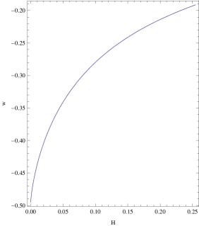
Figure 2: The variation of w𝑤w against H𝐻H for wm=.01,n=.5,ρcard=.1,Λ=.01,ρ0=.001,k=1,l=.9,H0=72formulae-sequencesubscript𝑤𝑚.01formulae-sequence𝑛.5formulae-sequencesubscript𝜌𝑐𝑎𝑟𝑑.1formulae-sequenceΛ.01formulae-sequencesubscript𝜌0.001formulae-sequence𝑘1formulae-sequence𝑙.9subscript𝐻072w_{m}=.01,n=.5,\rho_{card}=.1,\Lambda=.01,\rho_{0}=.001,k=1,l=.9,H_{0}=72.
Refer to caption
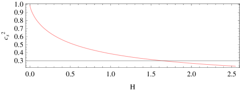
Figure 3: The variation of cs2superscriptsubscript𝑐𝑠2c_{s}^{2} against H𝐻H for wm=.01,n=.5,ρcard=.1,Λ=.01,ρ0=.001,k=1,l=.9,H0=72formulae-sequencesubscript𝑤𝑚.01formulae-sequence𝑛.5formulae-sequencesubscript𝜌𝑐𝑎𝑟𝑑.1formulae-sequenceΛ.01formulae-sequencesubscript𝜌0.001formulae-sequence𝑘1formulae-sequence𝑙.9subscript𝐻072w_{m}=.01,n=.5,\rho_{card}=.1,\Lambda=.01,\rho_{0}=.001,k=1,l=.9,H_{0}=72.
Refer to caption
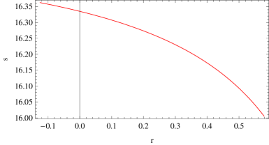
Figure 4: The variation of s𝑠s against r𝑟r for wm=.01,n=.5,ρcard=.1,Λ=.01,ρ0=.001,k=1,l=.9,H0=72formulae-sequencesubscript𝑤𝑚.01formulae-sequence𝑛.5formulae-sequencesubscript𝜌𝑐𝑎𝑟𝑑.1formulae-sequenceΛ.01formulae-sequencesubscript𝜌0.001formulae-sequence𝑘1formulae-sequence𝑙.9subscript𝐻072w_{m}=.01,n=.5,\rho_{card}=.1,\Lambda=.01,\rho_{0}=.001,k=1,l=.9,H_{0}=72.
Refer to caption
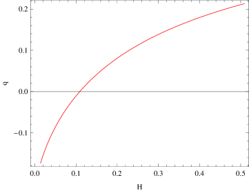
Figure 5: The variation of q𝑞q against H𝐻H for wm=.01,n=.5,ρcard=.1,Λ=.01,ρ0=.001,k=1,l=.9,H0=72formulae-sequencesubscript𝑤𝑚.01formulae-sequence𝑛.5formulae-sequencesubscript𝜌𝑐𝑎𝑟𝑑.1formulae-sequenceΛ.01formulae-sequencesubscript𝜌0.001formulae-sequence𝑘1formulae-sequence𝑙.9subscript𝐻072w_{m}=.01,n=.5,\rho_{card}=.1,\Lambda=.01,\rho_{0}=.001,k=1,l=.9,H_{0}=72.
Refer to caption
Figure 6: The variation of Om𝑂𝑚Om against H𝐻H for wm=.01,n=.5,ρcard=.1,Λ=.01,ρ0=.001,k=1,l=.9,H0=72formulae-sequencesubscript𝑤𝑚.01formulae-sequence𝑛.5formulae-sequencesubscript𝜌𝑐𝑎𝑟𝑑.1formulae-sequenceΛ.01formulae-sequencesubscript𝜌0.001formulae-sequence𝑘1formulae-sequence𝑙.9subscript𝐻072w_{m}=.01,n=.5,\rho_{card}=.1,\Lambda=.01,\rho_{0}=.001,k=1,l=.9,H_{0}=72.

From above, we see that wcsubscript𝑤𝑐w_{c} is a constant. From (16), (18), (19), (20), (23) and (24) we get the statefinder parameters and deceleration parameter,

r=(1+z)3ρ0(2+9wm(1+wm))+(1+z)3wm((1+z)3(1+wm)ρ0ρcard)nρcard(2+9n(1+wm)(1+n+nwm))2(1+z)3ρ0+2(1+z)3wm((1+z)3(1+wm)ρ0ρcard)nρcard𝑟superscript1𝑧3subscript𝜌029subscript𝑤𝑚1subscript𝑤𝑚superscript1𝑧3subscript𝑤𝑚superscriptsuperscript1𝑧31subscript𝑤𝑚subscript𝜌0subscript𝜌𝑐𝑎𝑟𝑑𝑛subscript𝜌𝑐𝑎𝑟𝑑29𝑛1subscript𝑤𝑚1𝑛𝑛subscript𝑤𝑚2superscript1𝑧3subscript𝜌02superscript1𝑧3subscript𝑤𝑚superscriptsuperscript1𝑧31subscript𝑤𝑚subscript𝜌0subscript𝜌𝑐𝑎𝑟𝑑𝑛subscript𝜌𝑐𝑎𝑟𝑑r=\frac{(1+z)^{3}\rho_{0}(2+9w_{m}(1+w_{m}))+(1+z)^{-3w_{m}}\left(\frac{(1+z)^{3(1+w_{m})}\rho_{0}}{\rho_{card}}\right)^{n}\rho_{card}(2+9n(1+w_{m})(-1+n+nw_{m}))}{2(1+z)^{3}\rho_{0}+2(1+z)^{-3w_{m}}\left(\frac{(1+z)^{3(1+w_{m})}\rho_{0}}{\rho_{card}}\right)^{n}\rho_{card}} (27)

and

s=(1+z)3ρ0wm(11+9wm)+(1+z)3wm((1+z)3(1+wm)ρ0ρcard)nρcard(1+n+nwm)(2+9n(1+wm))2(1+z)3ρ0wm+2(1+z)3wm((1+z)3(1+wm)ρ0ρcard)nρcard(1+n+nwm)𝑠superscript1𝑧3subscript𝜌0subscript𝑤𝑚119subscript𝑤𝑚superscript1𝑧3subscript𝑤𝑚superscriptsuperscript1𝑧31subscript𝑤𝑚subscript𝜌0subscript𝜌𝑐𝑎𝑟𝑑𝑛subscript𝜌𝑐𝑎𝑟𝑑1𝑛𝑛subscript𝑤𝑚29𝑛1subscript𝑤𝑚2superscript1𝑧3subscript𝜌0subscript𝑤𝑚2superscript1𝑧3subscript𝑤𝑚superscriptsuperscript1𝑧31subscript𝑤𝑚subscript𝜌0subscript𝜌𝑐𝑎𝑟𝑑𝑛subscript𝜌𝑐𝑎𝑟𝑑1𝑛𝑛subscript𝑤𝑚s=\frac{(1+z)^{3}\rho_{0}w_{m}(11+9w_{m})+(1+z)^{-3w_{m}}\left(\frac{(1+z)^{3(1+w_{m})}\rho_{0}}{\rho_{card}}\right)^{n}\rho_{card}(-1+n+nw_{m})(2+9n(1+w_{m}))}{2(1+z)^{3}\rho_{0}w_{m}+2(1+z)^{-3w_{m}}\left(\frac{(1+z)^{3(1+w_{m})}\rho_{0}}{\rho_{card}}\right)^{n}\rho_{card}(-1+n+nw_{m})} (28)
q=(1+z)3ρ0(1+3wm)+(1+z)3wm((1+z)3(1+wm)ρ0ρcard)nρcard(2+3n(1+wm))2(1+z)3ρ0+2(1+z)3wm((1+z)3(1+wm)ρ0ρcard)nρcard𝑞superscript1𝑧3subscript𝜌013subscript𝑤𝑚superscript1𝑧3subscript𝑤𝑚superscriptsuperscript1𝑧31subscript𝑤𝑚subscript𝜌0subscript𝜌𝑐𝑎𝑟𝑑𝑛subscript𝜌𝑐𝑎𝑟𝑑23𝑛1subscript𝑤𝑚2superscript1𝑧3subscript𝜌02superscript1𝑧3subscript𝑤𝑚superscriptsuperscript1𝑧31subscript𝑤𝑚subscript𝜌0subscript𝜌𝑐𝑎𝑟𝑑𝑛subscript𝜌𝑐𝑎𝑟𝑑q=\frac{(1+z)^{3}\rho_{0}(1+3w_{m})+(1+z)^{-3w_{m}}\left(\frac{(1+z)^{3(1+w_{m})}\rho_{0}}{\rho_{card}}\right)^{n}\rho_{card}(-2+3n(1+w_{m}))}{2(1+z)^{3}\rho_{0}+2(1+z)^{-3w_{m}}\left(\frac{(1+z)^{3(1+w_{m})}\rho_{0}}{\rho_{card}}\right)^{n}\rho_{card}} (29)

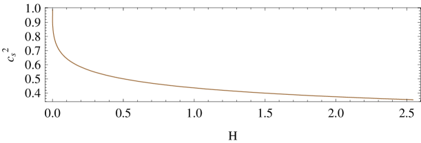
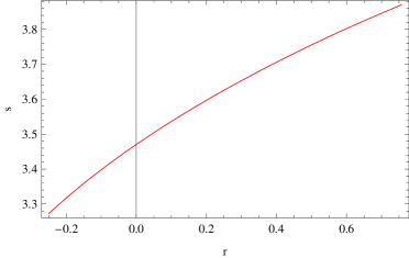
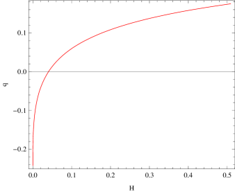
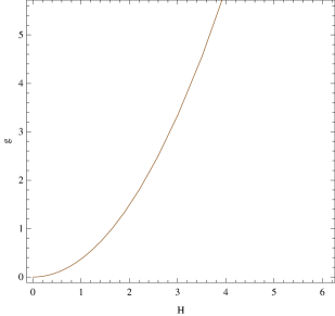
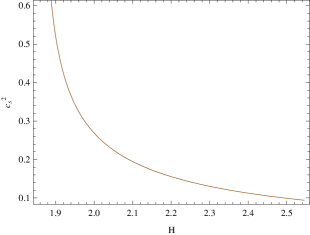
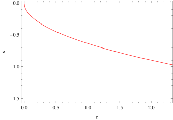
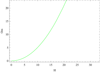
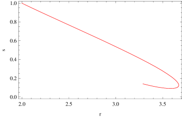
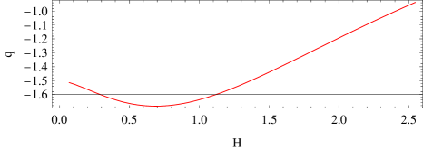
Fig.1  represents the variation of g𝑔g against H𝐻H, Fig.2  represents the variation of w𝑤w against H𝐻H. From (9), (10), (16), (23) and (24) we plot the graph which shows the variation of the square of velocity of sound cs2superscriptsubscript𝑐𝑠2c_{s}^{2} against H𝐻H is given in Fig.3. Fig.4  represents the variation of s𝑠s against r𝑟r and Fig.5  represents the variation of q𝑞q against H𝐻H. From (8), (21) and (22) we get the value of Om𝑂𝑚Om. Fig.6  represents the variation of Om𝑂𝑚Om against H𝐻H. The values are taken as, wm=.01,n=.5,ρcard=.1,Λ=.01,ρ0=.001,k=1,l=.9,H0=72formulae-sequencesubscript𝑤𝑚.01formulae-sequence𝑛.5formulae-sequencesubscript𝜌𝑐𝑎𝑟𝑑.1formulae-sequenceΛ.01formulae-sequencesubscript𝜌0.001formulae-sequence𝑘1formulae-sequence𝑙.9subscript𝐻072w_{m}=.01,n=.5,\rho_{card}=.1,\Lambda=.01,\rho_{0}=.001,k=1,l=.9,H_{0}=72. From the figures, we see that g,w,q𝑔𝑤𝑞g,w,q and Om𝑂𝑚Om decrease as H𝐻H decreases and cs2superscriptsubscript𝑐𝑠2c_{s}^{2} lies between 0 and 1. The parameter s𝑠s increases and keeps positive sign as r𝑟r decreases from positive to negative values.

IV.2 Modified Polytropic Model (MP)

Modified polytropic Cardassian model is a slight modification of the previous one, can be used on all scales, but it does not quite fit the criteria of the Cardassian model as defined above. At late times in the future of the Universe, when ρmρcardmuch-less-thansubscript𝜌𝑚subscript𝜌𝑐𝑎𝑟𝑑\rho_{m}\ll\rho_{card}, this model becomes cosmological constant dominated with Λ=ρcardΛsubscript𝜌𝑐𝑎𝑟𝑑\Lambda=\rho_{card}. This energy density is very similar to a model which motivated by gravitational leakage into extra dimensions. In this model g(ρ)𝑔𝜌g(\rho) is defined as [25],

g(ρ)=ρm[1+(ρcardρm)α(n1)]1α𝑔𝜌subscript𝜌𝑚superscriptdelimited-[]1superscriptsubscript𝜌𝑐𝑎𝑟𝑑subscript𝜌𝑚𝛼𝑛11𝛼g(\rho)=\rho_{m}\left[1+\left(\frac{\rho_{card}}{\rho_{m}}\right)^{\alpha(n-1)}\right]^{\frac{1}{\alpha}} (30)

where ρcardsubscript𝜌𝑐𝑎𝑟𝑑\rho_{card} is a characteristic constant energy density and α0𝛼0\alpha\neq 0 and n𝑛n are dimensionless positive constants. So from (9), (14), (16) and (30) we get,

ρc=(1+z)3(1+wm)ρ0(1+(1+XMP)1α)subscript𝜌𝑐superscript1𝑧31subscript𝑤𝑚subscript𝜌01superscript1subscript𝑋𝑀𝑃1𝛼\rho_{c}=(1+z)^{3(1+w_{m})}\rho_{0}(-1+(1+X_{MP})^{\frac{1}{\alpha}}) (31)

and

pc=(1+z)3(1+wm)ρ0(XMP(1+XMP)1+1αwm+(1+XMP)1+1α(wmXMP(n+(2+n)wm)))subscript𝑝𝑐superscript1𝑧31subscript𝑤𝑚subscript𝜌0subscript𝑋𝑀𝑃superscript1subscript𝑋𝑀𝑃11𝛼subscript𝑤𝑚superscript1subscript𝑋𝑀𝑃11𝛼subscript𝑤𝑚subscript𝑋𝑀𝑃𝑛2𝑛subscript𝑤𝑚p_{c}=(1+z)^{3(1+w_{m})}\rho_{0}(X_{MP}(1+X_{MP})^{-1+\frac{1}{\alpha}}-w_{m}+(1+X_{MP})^{-1+\frac{1}{\alpha}}(w_{m}-X_{MP}(n+(-2+n)w_{m}))) (32)

where,

XMP=[(1+z)3(1+wm)ρcardρ0](n1)αsubscript𝑋𝑀𝑃superscriptdelimited-[]superscript1𝑧31subscript𝑤𝑚subscript𝜌𝑐𝑎𝑟𝑑subscript𝜌0𝑛1𝛼X_{MP}=\left[\frac{(1+z)^{-3(1+w_{m})}\rho_{card}}{\rho_{0}}\right]^{(n-1)\alpha}
Refer to caption
Figure 7: The variation of g𝑔g against H𝐻H for α=.5,wm=.01,n=.5,ρcard=.1,Λ=.01,ρ0=.001,k=1,l=.9,H0=72formulae-sequence𝛼.5formulae-sequencesubscript𝑤𝑚.01formulae-sequence𝑛.5formulae-sequencesubscript𝜌𝑐𝑎𝑟𝑑.1formulae-sequenceΛ.01formulae-sequencesubscript𝜌0.001formulae-sequence𝑘1formulae-sequence𝑙.9subscript𝐻072\alpha=.5,w_{m}=.01,n=.5,\rho_{card}=.1,\Lambda=.01,\rho_{0}=.001,k=1,l=.9,H_{0}=72.
Refer to caption
Figure 8: The variation of wcsubscript𝑤𝑐w_{c} against H𝐻H for α=.5,wm=.01,n=.5,ρcard=.1,Λ=.01,ρ0=.001,k=1,l=.9,H0=72formulae-sequence𝛼.5formulae-sequencesubscript𝑤𝑚.01formulae-sequence𝑛.5formulae-sequencesubscript𝜌𝑐𝑎𝑟𝑑.1formulae-sequenceΛ.01formulae-sequencesubscript𝜌0.001formulae-sequence𝑘1formulae-sequence𝑙.9subscript𝐻072\alpha=.5,w_{m}=.01,n=.5,\rho_{card}=.1,\Lambda=.01,\rho_{0}=.001,k=1,l=.9,H_{0}=72.
Refer to caption
Figure 9: The variation of w𝑤w against H𝐻H for α=.5,wm=.01,n=.5,ρcard=.1,Λ=.01,ρ0=.001,k=1,l=.9,H0=72formulae-sequence𝛼.5formulae-sequencesubscript𝑤𝑚.01formulae-sequence𝑛.5formulae-sequencesubscript𝜌𝑐𝑎𝑟𝑑.1formulae-sequenceΛ.01formulae-sequencesubscript𝜌0.001formulae-sequence𝑘1formulae-sequence𝑙.9subscript𝐻072\alpha=.5,w_{m}=.01,n=.5,\rho_{card}=.1,\Lambda=.01,\rho_{0}=.001,k=1,l=.9,H_{0}=72.
Refer to caption
Figure 10: The variation of cs2superscriptsubscript𝑐𝑠2c_{s}^{2} against H𝐻H for α=.5,wm=.01,n=.5,ρcard=.1,Λ=.01,ρ0=.001,k=1,l=.9,H0=72formulae-sequence𝛼.5formulae-sequencesubscript𝑤𝑚.01formulae-sequence𝑛.5formulae-sequencesubscript𝜌𝑐𝑎𝑟𝑑.1formulae-sequenceΛ.01formulae-sequencesubscript𝜌0.001formulae-sequence𝑘1formulae-sequence𝑙.9subscript𝐻072\alpha=.5,w_{m}=.01,n=.5,\rho_{card}=.1,\Lambda=.01,\rho_{0}=.001,k=1,l=.9,H_{0}=72.
Refer to caption
Figure 11: The variation of s𝑠s against r𝑟r for α=.5,wm=.01,n=.5,ρcard=.1,Λ=.01,ρ0=.001,k=1,l=.9,H0=72formulae-sequence𝛼.5formulae-sequencesubscript𝑤𝑚.01formulae-sequence𝑛.5formulae-sequencesubscript𝜌𝑐𝑎𝑟𝑑.1formulae-sequenceΛ.01formulae-sequencesubscript𝜌0.001formulae-sequence𝑘1formulae-sequence𝑙.9subscript𝐻072\alpha=.5,w_{m}=.01,n=.5,\rho_{card}=.1,\Lambda=.01,\rho_{0}=.001,k=1,l=.9,H_{0}=72.
Refer to caption
Figure 12: The variation of q𝑞q against H𝐻H for α=.5,wm=.01,n=.5,ρcard=.1,Λ=.01,ρ0=.001,k=1,l=.9,H0=72formulae-sequence𝛼.5formulae-sequencesubscript𝑤𝑚.01formulae-sequence𝑛.5formulae-sequencesubscript𝜌𝑐𝑎𝑟𝑑.1formulae-sequenceΛ.01formulae-sequencesubscript𝜌0.001formulae-sequence𝑘1formulae-sequence𝑙.9subscript𝐻072\alpha=.5,w_{m}=.01,n=.5,\rho_{card}=.1,\Lambda=.01,\rho_{0}=.001,k=1,l=.9,H_{0}=72.
Refer to caption
Figure 13: The variation of Om𝑂𝑚Om against H𝐻H for α=.5,wm=.01,n=.5,ρcard=.1,Λ=.01,ρ0=.001,k=1,l=.9,H0=72formulae-sequence𝛼.5formulae-sequencesubscript𝑤𝑚.01formulae-sequence𝑛.5formulae-sequencesubscript𝜌𝑐𝑎𝑟𝑑.1formulae-sequenceΛ.01formulae-sequencesubscript𝜌0.001formulae-sequence𝑘1formulae-sequence𝑙.9subscript𝐻072\alpha=.5,w_{m}=.01,n=.5,\rho_{card}=.1,\Lambda=.01,\rho_{0}=.001,k=1,l=.9,H_{0}=72.

So the equation of state is given by,

wc=(1+z)3(1+wm)ρ0(XMP(1+XMP)1+1αwm+(1+XMP)1+1α(wmXMP(n+(2+n)wm)))(1+z)3(1+wm)ρ0(1+(1+XMP)1α)subscript𝑤𝑐superscript1𝑧31subscript𝑤𝑚subscript𝜌0subscript𝑋𝑀𝑃superscript1subscript𝑋𝑀𝑃11𝛼subscript𝑤𝑚superscript1subscript𝑋𝑀𝑃11𝛼subscript𝑤𝑚subscript𝑋𝑀𝑃𝑛2𝑛subscript𝑤𝑚superscript1𝑧31subscript𝑤𝑚subscript𝜌01superscript1subscript𝑋𝑀𝑃1𝛼w_{c}=\frac{(1+z)^{3(1+w_{m})}\rho_{0}(X_{MP}(1+X_{MP})^{-1+\frac{1}{\alpha}}-w_{m}+(1+X_{MP})^{-1+\frac{1}{\alpha}}(w_{m}-X_{MP}(n+(-2+n)w_{m})))}{(1+z)^{3(1+w_{m})}\rho_{0}(-1+(1+X_{MP})^{\frac{1}{\alpha}})} (33)

and

w=ρ0wm(1+z)3(1+wm)+(1+z)3(1+wm)ρ0(XMP(1+XMP)1+1αwm+(1+XMP)1+1α(wmXMP(n+(2+n)wm)))ρ0(1+z)3(1+wm)+(1+z)3(1+wm)ρ0(1+(1+XMP)1α)𝑤subscript𝜌0subscript𝑤𝑚superscript1𝑧31subscript𝑤𝑚superscript1𝑧31subscript𝑤𝑚subscript𝜌0subscript𝑋𝑀𝑃superscript1subscript𝑋𝑀𝑃11𝛼subscript𝑤𝑚superscript1subscript𝑋𝑀𝑃11𝛼subscript𝑤𝑚subscript𝑋𝑀𝑃𝑛2𝑛subscript𝑤𝑚subscript𝜌0superscript1𝑧31subscript𝑤𝑚superscript1𝑧31subscript𝑤𝑚subscript𝜌01superscript1subscript𝑋𝑀𝑃1𝛼w=\frac{\rho_{0}w_{m}(1+z)^{3(1+w_{m})}+(1+z)^{3(1+w_{m})}\rho_{0}(X_{MP}(1+X_{MP})^{-1+\frac{1}{\alpha}}-w_{m}+(1+X_{MP})^{-1+\frac{1}{\alpha}}(w_{m}-X_{MP}(n+(-2+n)w_{m})))}{\rho_{0}(1+z)^{3(1+w_{m})}+(1+z)^{3(1+w_{m})}\rho_{0}(-1+(1+X_{MP})^{\frac{1}{\alpha}})} (34)

From (16), (18), (19), (20), (31) and (32) we get the statefinder parameters and deceleration parameter,

r=[2+9wm+9wm2+XMP(56wm+3n(1+wm))(46wm+3n(1+wm))+XMP(13+9α(1+wm)2\displaystyle r=\left[2+9w_{m}+9w_{m}^{2}+X_{MP}(-5-6w_{m}+3n(1+w_{m}))(-4-6w_{m}+3n(1+w_{m}))+X_{MP}(13+9\alpha(1+w_{m})^{2}\right.
+9n2α(1+wm)2+9wm(5+4wm)9n(1+wm)(1+2wm+2α(1+wm)))]/[2(1+XMP)2]\left.+9n^{2}\alpha(1+w_{m})^{2}+9w_{m}(5+4w_{m})-9n(1+w_{m})(1+2w_{m}+2\alpha(1+w_{m})))\right]/\left[2(1+X_{MP})^{2}\right] (35)

and

s=12[209n+18wm9nwm9(1+n)(1+α)(1+wm)1+XMP9(1+n)αwm(1+wm)wm+XMP(1+n+(2+n)wm)]𝑠12delimited-[]209𝑛18subscript𝑤𝑚9𝑛subscript𝑤𝑚91𝑛1𝛼1subscript𝑤𝑚1subscript𝑋𝑀𝑃91𝑛𝛼subscript𝑤𝑚1subscript𝑤𝑚subscript𝑤𝑚subscript𝑋𝑀𝑃1𝑛2𝑛subscript𝑤𝑚s=\frac{1}{2}\left[20-9n+18w_{m}-9nw_{m}-\frac{9(-1+n)(-1+\alpha)(1+w_{m})}{1+X_{MP}}-\frac{9(-1+n)\alpha w_{m}(1+w_{m})}{-w_{m}+X_{MP}(-1+n+(-2+n)w_{m})}\right] (36)
q=12[43n+6wm3nwm+3(1+n)(1+wm)1+XMP]𝑞12delimited-[]43𝑛6subscript𝑤𝑚3𝑛subscript𝑤𝑚31𝑛1subscript𝑤𝑚1subscript𝑋𝑀𝑃q=\frac{1}{2}\left[4-3n+6w_{m}-3nw_{m}+\frac{3(-1+n)(1+w_{m})}{1+X_{MP}}\right] (37)

Fig.7, 8 and 9  represents the variation of g𝑔g, wcsubscript𝑤𝑐w_{c} and w𝑤w against H𝐻H respectively. From (9), (10), (16), (31) and (32) we plot the graph which shows the variation of the square of velocity of sound cs2superscriptsubscript𝑐𝑠2c_{s}^{2} against H𝐻H is given in Fig. 10, Fig.11  represents the variation of s𝑠s against r𝑟r and Fig.12  represents the variation of q𝑞q against H𝐻H. From (8), (21) and (30) we get the value of Om𝑂𝑚Om. Fig.13  represents the variation of Om𝑂𝑚Om against H𝐻H. The value of parameters are taken as, α=.5,wm=.01,n=.5,ρcard=.1,Λ=.01,ρ0=.001,k=1,l=.9,H0=72formulae-sequence𝛼.5formulae-sequencesubscript𝑤𝑚.01formulae-sequence𝑛.5formulae-sequencesubscript𝜌𝑐𝑎𝑟𝑑.1formulae-sequenceΛ.01formulae-sequencesubscript𝜌0.001formulae-sequence𝑘1formulae-sequence𝑙.9subscript𝐻072\alpha=.5,w_{m}=.01,n=.5,\rho_{card}=.1,\Lambda=.01,\rho_{0}=.001,k=1,l=.9,H_{0}=72. From the figures, we see that g,wc,w,q𝑔subscript𝑤𝑐𝑤𝑞g,w_{c},w,q and Om𝑂𝑚Om decrease as H𝐻H decreases and cs2superscriptsubscript𝑐𝑠2c_{s}^{2} lies between 0 and 1. The parameter s𝑠s decreases and keeps positive sign as r𝑟r decreases from positive to negative values.

IV.3 Exponential Model:-

In this model g(ρ)𝑔𝜌g(\rho) is defined as [26],

g(ρ)=ρmexp[(ρcardρm)n]𝑔𝜌subscript𝜌𝑚𝑒𝑥𝑝delimited-[]superscriptsubscript𝜌𝑐𝑎𝑟𝑑subscript𝜌𝑚𝑛g(\rho)=\rho_{m}~{}exp\left[\left(\frac{\rho_{card}}{\rho_{m}}\right)^{n}\right] (38)

where ρcardsubscript𝜌𝑐𝑎𝑟𝑑\rho_{card} is a characteristic constant energy density and n𝑛n is a dimensionless positive constants. So from (9), (14), (16) and (38) we get,

ρc=(1+eXExp)(1+z)3(1+wm)ρ0subscript𝜌𝑐1superscript𝑒subscript𝑋𝐸𝑥𝑝superscript1𝑧31subscript𝑤𝑚subscript𝜌0\rho_{c}=(-1+e^{X_{Exp}})(1+z)^{3(1+w_{m})}\rho_{0} (39)

and

pc=(1+z)3(1+wm)ρ0(wm+eXExp(wm+nXExp(1+wm)))subscript𝑝𝑐superscript1𝑧31subscript𝑤𝑚subscript𝜌0subscript𝑤𝑚superscript𝑒subscript𝑋𝐸𝑥𝑝subscript𝑤𝑚𝑛subscript𝑋𝐸𝑥𝑝1subscript𝑤𝑚p_{c}=-(1+z)^{3(1+w_{m})}\rho_{0}(w_{m}+e^{X_{Exp}}(-w_{m}+nX_{Exp}(1+w_{m}))) (40)

where,

XExp=[(1+z)3(1+wm)ρcardρ0]nsubscript𝑋𝐸𝑥𝑝superscriptdelimited-[]superscript1𝑧31subscript𝑤𝑚subscript𝜌𝑐𝑎𝑟𝑑subscript𝜌0𝑛X_{Exp}=\left[\frac{(1+z)^{-3(1+w_{m})}\rho_{card}}{\rho_{0}}\right]^{n}

So the equation of state is given by,

wc=(1+z)3(1+wm)ρ0(wm+eXExp(wm+nXExp(1+wm)))(1+eXExp)(1+z)3(1+wm)ρ0subscript𝑤𝑐superscript1𝑧31subscript𝑤𝑚subscript𝜌0subscript𝑤𝑚superscript𝑒subscript𝑋𝐸𝑥𝑝subscript𝑤𝑚𝑛subscript𝑋𝐸𝑥𝑝1subscript𝑤𝑚1superscript𝑒subscript𝑋𝐸𝑥𝑝superscript1𝑧31subscript𝑤𝑚subscript𝜌0w_{c}=\frac{-(1+z)^{3(1+w_{m})}\rho_{0}(w_{m}+e^{X_{Exp}}(-w_{m}+nX_{Exp}(1+w_{m})))}{(-1+e^{X_{Exp}})(1+z)^{3(1+w_{m})}\rho_{0}} (41)

and

w=ρ0w0(1+z)3(1+wm)(1+z)3(1+wm)ρ0(wm+eXExp(wm+nXExp(1+wm)))ρ0(1+z)3(1+wm)+(1+eXExp)(1+z)3(1+wm)ρ0𝑤subscript𝜌0subscript𝑤0superscript1𝑧31subscript𝑤𝑚superscript1𝑧31subscript𝑤𝑚subscript𝜌0subscript𝑤𝑚superscript𝑒subscript𝑋𝐸𝑥𝑝subscript𝑤𝑚𝑛subscript𝑋𝐸𝑥𝑝1subscript𝑤𝑚subscript𝜌0superscript1𝑧31subscript𝑤𝑚1superscript𝑒subscript𝑋𝐸𝑥𝑝superscript1𝑧31subscript𝑤𝑚subscript𝜌0w=\frac{\rho_{0}w_{0}(1+z)^{3(1+w_{m})}-(1+z)^{3(1+w_{m})}\rho_{0}(w_{m}+e^{X_{Exp}}(-w_{m}+nX_{Exp}(1+w_{m})))}{\rho_{0}(1+z)^{3(1+w_{m})}+(-1+e^{X_{Exp}})(1+z)^{3(1+w_{m})}\rho_{0}} (42)

From (16), (18), (19), (20), (39) and (40) we get the statefinder parameters and deceleration parameter,

r=12(2+9wm+9(wm2+n2XExp2(1+wm)2+nXExp(1+wm)(1+n+(2+n)wm)))𝑟1229subscript𝑤𝑚9superscriptsubscript𝑤𝑚2superscript𝑛2superscriptsubscript𝑋𝐸𝑥𝑝2superscript1subscript𝑤𝑚2𝑛subscript𝑋𝐸𝑥𝑝1subscript𝑤𝑚1𝑛2𝑛subscript𝑤𝑚r=\frac{1}{2}\left(2+9w_{m}+9(w_{m}^{2}+n^{2}X_{Exp}^{2}(1+w_{m})^{2}+nX_{Exp}(1+w_{m})(-1+n+(-2+n)w_{m}))\right) (43)

and

s=12(119n+9wm9nwm9nXExp(1+wm)9nwm(1+wm)wm+nXExp(1+wm))𝑠12119𝑛9subscript𝑤𝑚9𝑛subscript𝑤𝑚9𝑛subscript𝑋𝐸𝑥𝑝1subscript𝑤𝑚9𝑛subscript𝑤𝑚1subscript𝑤𝑚subscript𝑤𝑚𝑛subscript𝑋𝐸𝑥𝑝1subscript𝑤𝑚s=\frac{1}{2}\left(11-9n+9w_{m}-9nw_{m}-9nX_{Exp}(1+w_{m})-\frac{9nw_{m}(1+w_{m})}{-w_{m}+nX_{Exp}(1+w_{m})}\right) (44)
q=12[1+3wm3nXExp(1+wm)]𝑞12delimited-[]13subscript𝑤𝑚3𝑛subscript𝑋𝐸𝑥𝑝1subscript𝑤𝑚q=\frac{1}{2}\left[1+3w_{m}-3nX_{Exp}(1+w_{m})\right] (45)
Refer to caption
Figure 14: The variation of w𝑤w against H𝐻H for wm=.01,n=2,ρcard=.1,Λ=.01,ρ0=.001,k=1,l=.9,H0=72formulae-sequencesubscript𝑤𝑚.01formulae-sequence𝑛2formulae-sequencesubscript𝜌𝑐𝑎𝑟𝑑.1formulae-sequenceΛ.01formulae-sequencesubscript𝜌0.001formulae-sequence𝑘1formulae-sequence𝑙.9subscript𝐻072w_{m}=.01,n=2,\rho_{card}=.1,\Lambda=.01,\rho_{0}=.001,k=1,l=.9,H_{0}=72.
Refer to caption
Figure 15: The variation of w𝑤w against z𝑧z for wm=.01,n=2,ρcard=.1,Λ=.01,ρ0=.001,k=1,l=.9,H0=72formulae-sequencesubscript𝑤𝑚.01formulae-sequence𝑛2formulae-sequencesubscript𝜌𝑐𝑎𝑟𝑑.1formulae-sequenceΛ.01formulae-sequencesubscript𝜌0.001formulae-sequence𝑘1formulae-sequence𝑙.9subscript𝐻072w_{m}=.01,n=2,\rho_{card}=.1,\Lambda=.01,\rho_{0}=.001,k=1,l=.9,H_{0}=72.
Refer to caption
Figure 16: The variation of w𝑤w against z𝑧z for wm=.01,n=2,ρcard=.1,Λ=.01,ρ0=.001,k=1,l=.9,H0=72formulae-sequencesubscript𝑤𝑚.01formulae-sequence𝑛2formulae-sequencesubscript𝜌𝑐𝑎𝑟𝑑.1formulae-sequenceΛ.01formulae-sequencesubscript𝜌0.001formulae-sequence𝑘1formulae-sequence𝑙.9subscript𝐻072w_{m}=.01,n=2,\rho_{card}=.1,\Lambda=.01,\rho_{0}=.001,k=1,l=.9,H_{0}=72.
Refer to caption
Figure 17: The variation of cs2superscriptsubscript𝑐𝑠2c_{s}^{2} against H𝐻H for wm=.01,n=2,ρcard=.1,Λ=.01,ρ0=.001,k=1,l=.9,H0=72formulae-sequencesubscript𝑤𝑚.01formulae-sequence𝑛2formulae-sequencesubscript𝜌𝑐𝑎𝑟𝑑.1formulae-sequenceΛ.01formulae-sequencesubscript𝜌0.001formulae-sequence𝑘1formulae-sequence𝑙.9subscript𝐻072w_{m}=.01,n=2,\rho_{card}=.1,\Lambda=.01,\rho_{0}=.001,k=1,l=.9,H_{0}=72.
Refer to caption
Figure 18: The variation of s𝑠s against r𝑟r for wm=.01,n=2,ρcard=.1,Λ=.01,ρ0=.001,k=1,l=.9,H0=72formulae-sequencesubscript𝑤𝑚.01formulae-sequence𝑛2formulae-sequencesubscript𝜌𝑐𝑎𝑟𝑑.1formulae-sequenceΛ.01formulae-sequencesubscript𝜌0.001formulae-sequence𝑘1formulae-sequence𝑙.9subscript𝐻072w_{m}=.01,n=2,\rho_{card}=.1,\Lambda=.01,\rho_{0}=.001,k=1,l=.9,H_{0}=72.
Refer to caption
Figure 19: The variation of q𝑞q against z𝑧z for wm=.01,n=2,ρcard=.1,Λ=.01,ρ0=.001,k=1,l=.9,H0=72formulae-sequencesubscript𝑤𝑚.01formulae-sequence𝑛2formulae-sequencesubscript𝜌𝑐𝑎𝑟𝑑.1formulae-sequenceΛ.01formulae-sequencesubscript𝜌0.001formulae-sequence𝑘1formulae-sequence𝑙.9subscript𝐻072w_{m}=.01,n=2,\rho_{card}=.1,\Lambda=.01,\rho_{0}=.001,k=1,l=.9,H_{0}=72.
Refer to caption
Figure 20: The variation of Om𝑂𝑚Om against H𝐻H for wm=.01,n=2,ρcard=.1,Λ=.01,ρ0=.001,k=1,l=.9,H0=72formulae-sequencesubscript𝑤𝑚.01formulae-sequence𝑛2formulae-sequencesubscript𝜌𝑐𝑎𝑟𝑑.1formulae-sequenceΛ.01formulae-sequencesubscript𝜌0.001formulae-sequence𝑘1formulae-sequence𝑙.9subscript𝐻072w_{m}=.01,n=2,\rho_{card}=.1,\Lambda=.01,\rho_{0}=.001,k=1,l=.9,H_{0}=72.

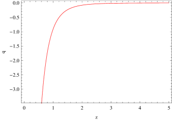
Fig.14, 15 and 16  represents the variation of g𝑔g, wcsubscript𝑤𝑐w_{c} and w𝑤w against H𝐻H, z𝑧z and z𝑧z respectively. From (9), (10), (16), (39) and (40) we plot the graph which shows the variation of the square of velocity of sound cs2superscriptsubscript𝑐𝑠2c_{s}^{2} against H𝐻H is given in Fig. 17. Fig.18  represents the variation of s𝑠s against r𝑟r and Fig.19  represents the variation of q𝑞q against H𝐻H. From (8), (21) and (38) we get the value of Om. Fig.20  represents the variation of Om𝑂𝑚Om against H𝐻H. The values are taken as, wm=.01,n=2,ρcard=.1,Λ=.01,ρ0=.001,k=1,l=.9,H0=72formulae-sequencesubscript𝑤𝑚.01formulae-sequence𝑛2formulae-sequencesubscript𝜌𝑐𝑎𝑟𝑑.1formulae-sequenceΛ.01formulae-sequencesubscript𝜌0.001formulae-sequence𝑘1formulae-sequence𝑙.9subscript𝐻072w_{m}=.01,n=2,\rho_{card}=.1,\Lambda=.01,\rho_{0}=.001,k=1,l=.9,H_{0}=72. From the figures, we see that g,wc,w,q𝑔subscript𝑤𝑐𝑤𝑞g,w_{c},w,q and Om𝑂𝑚Om decrease as H𝐻H decreases and cs2superscriptsubscript𝑐𝑠2c_{s}^{2} lies between 0 and 1. The parameter s𝑠s increases and keeps negative sign as r𝑟r decreases.

IV.4 Modified Exponential Model

In this model g(ρ)𝑔𝜌g(\rho) is defined as [26],

g(ρ)=(ρm+ρcard)exp[(αρcardρm+ρcard)n]𝑔𝜌subscript𝜌𝑚subscript𝜌𝑐𝑎𝑟𝑑𝑒𝑥𝑝delimited-[]superscript𝛼subscript𝜌𝑐𝑎𝑟𝑑subscript𝜌𝑚subscript𝜌𝑐𝑎𝑟𝑑𝑛g(\rho)=(\rho_{m}+\rho_{card})~{}exp\left[\left(\frac{\alpha\rho_{card}}{\rho_{m}+\rho_{card}}\right)^{n}\right] (46)

where ρcardsubscript𝜌𝑐𝑎𝑟𝑑\rho_{card} is a characteristic constant energy density and α𝛼\alpha and n𝑛n are dimensionless positive constants. So from (9), (14), (16) and (46) we get,

ρc=(1+z)3(1+wm)ρ0+e(αρcard(1+z)3(1+wm)ρ0+ρcard)n((1+z)3(1+wm)ρ0+ρcard)subscript𝜌𝑐superscript1𝑧31subscript𝑤𝑚subscript𝜌0superscript𝑒superscript𝛼subscript𝜌𝑐𝑎𝑟𝑑superscript1𝑧31subscript𝑤𝑚subscript𝜌0subscript𝜌𝑐𝑎𝑟𝑑𝑛superscript1𝑧31subscript𝑤𝑚subscript𝜌0subscript𝜌𝑐𝑎𝑟𝑑\rho_{c}=-(1+z)^{3(1+w_{m})}\rho_{0}+e^{\left(\frac{\alpha\rho_{card}}{(1+z)^{3(1+w_{m})}\rho_{0}+\rho_{card}}\right)^{n}}((1+z)^{3(1+w_{m})}\rho_{0}+\rho_{card}) (47)

and

pc=(1+z)3wm((1+z)3ρ0wmeXME((1+z)3wmρcard+(1+z)3ρ0(wm+nXME)n(1+wm))))p_{c}=(1+z)^{3w_{m}}(-(1+z)^{3}\rho_{0}w_{m}-e^{X_{ME}}((1+z)^{-3w_{m}}\rho_{card}+(1+z)^{3}\rho_{0}(-w_{m}+nX_{ME})^{n}(1+w_{m})))) (48)

So the equation of state is given by,

wc=(1+z)3wm((1+z)3ρ0wmeXME((1+z)3wmρcard+(1+z)3ρ0(wm+nXME(1+wm))))(1+z)3(1+wm)ρ0+eXME((1+z)3(1+wm)ρ0+ρcard)subscript𝑤𝑐superscript1𝑧3subscript𝑤𝑚superscript1𝑧3subscript𝜌0subscript𝑤𝑚superscript𝑒subscript𝑋𝑀𝐸superscript1𝑧3subscript𝑤𝑚subscript𝜌𝑐𝑎𝑟𝑑superscript1𝑧3subscript𝜌0subscript𝑤𝑚𝑛subscript𝑋𝑀𝐸1subscript𝑤𝑚superscript1𝑧31subscript𝑤𝑚subscript𝜌0superscript𝑒subscript𝑋𝑀𝐸superscript1𝑧31subscript𝑤𝑚subscript𝜌0subscript𝜌𝑐𝑎𝑟𝑑w_{c}=\frac{(1+z)^{3w_{m}}(-(1+z)^{3}\rho_{0}w_{m}-e^{X_{ME}}((1+z)^{-3w_{m}}\rho_{card}+(1+z)^{3}\rho_{0}(-w_{m}+nX_{ME}(1+w_{m}))))}{-(1+z)^{3(1+w_{m})}\rho_{0}+e^{X_{ME}}((1+z)^{3(1+w_{m})}\rho_{0}+\rho_{card})} (49)

and

w=wmρ0(1+z)3(1+wm)+(1+z)3wm((1+z)3ρ0wmeXME((1+z)3wmρcard+(1+z)3ρ0(wm+nXME(1+wm))))ρ0(1+z)3(1+wm)(1+z)3(1+wm)ρ0+eXME((1+z)3(1+wm)ρ0+ρcard)𝑤subscript𝑤𝑚subscript𝜌0superscript1𝑧31subscript𝑤𝑚superscript1𝑧3subscript𝑤𝑚superscript1𝑧3subscript𝜌0subscript𝑤𝑚superscript𝑒subscript𝑋𝑀𝐸superscript1𝑧3subscript𝑤𝑚subscript𝜌𝑐𝑎𝑟𝑑superscript1𝑧3subscript𝜌0subscript𝑤𝑚𝑛subscript𝑋𝑀𝐸1subscript𝑤𝑚subscript𝜌0superscript1𝑧31subscript𝑤𝑚superscript1𝑧31subscript𝑤𝑚subscript𝜌0superscript𝑒subscript𝑋𝑀𝐸superscript1𝑧31subscript𝑤𝑚subscript𝜌0subscript𝜌𝑐𝑎𝑟𝑑w=\frac{w_{m}\rho_{0}(1+z)^{3(1+w_{m})}+(1+z)^{3w_{m}}(-(1+z)^{3}\rho_{0}w_{m}-e^{X_{ME}}((1+z)^{-3w_{m}}\rho_{card}+(1+z)^{3}\rho_{0}(-w_{m}+nX_{ME}(1+w_{m}))))}{\rho_{0}(1+z)^{3(1+w_{m})}-(1+z)^{3(1+w_{m})}\rho_{0}+e^{X_{ME}}((1+z)^{3(1+w_{m})}\rho_{0}+\rho_{card})} (50)

where

XME=(αρcard(1+z)3(1+wm)ρ0+ρcard)nsubscript𝑋𝑀𝐸superscript𝛼subscript𝜌𝑐𝑎𝑟𝑑superscript1𝑧31subscript𝑤𝑚subscript𝜌0subscript𝜌𝑐𝑎𝑟𝑑𝑛X_{ME}=\left(\frac{\alpha\rho_{card}}{(1+z)^{3(1+w_{m})}\rho_{0}+\rho_{card}}\right)^{n}
Refer to caption
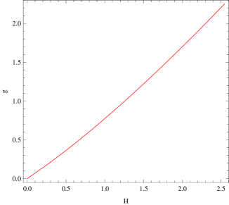
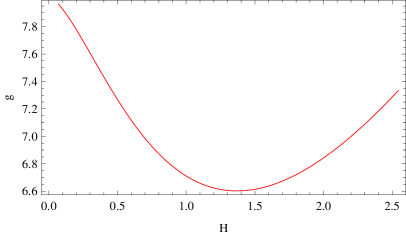
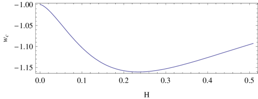
Figure 21: The variation of wcsubscript𝑤𝑐w_{c} against H𝐻H for α=2.5,wm=.01,n=.8,ρcard=.1,Λ=.01,ρ0=.001,k=1,l=.9,H0=72formulae-sequence𝛼2.5formulae-sequencesubscript𝑤𝑚.01formulae-sequence𝑛.8formulae-sequencesubscript𝜌𝑐𝑎𝑟𝑑.1formulae-sequenceΛ.01formulae-sequencesubscript𝜌0.001formulae-sequence𝑘1formulae-sequence𝑙.9subscript𝐻072\alpha=2.5,w_{m}=.01,n=.8,\rho_{card}=.1,\Lambda=.01,\rho_{0}=.001,k=1,l=.9,H_{0}=72.
Refer to caption
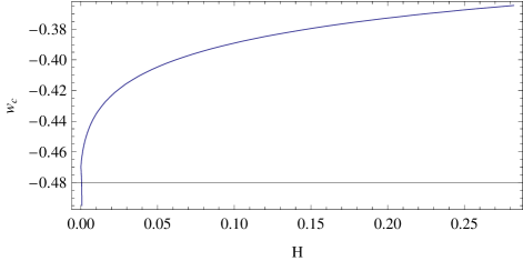
Figure 22: The variation of wcsubscript𝑤𝑐w_{c} against H𝐻H for α=2.5,wm=.01,n=.8,ρcard=.1,Λ=.01,ρ0=.001,k=1,l=.9,H0=72formulae-sequence𝛼2.5formulae-sequencesubscript𝑤𝑚.01formulae-sequence𝑛.8formulae-sequencesubscript𝜌𝑐𝑎𝑟𝑑.1formulae-sequenceΛ.01formulae-sequencesubscript𝜌0.001formulae-sequence𝑘1formulae-sequence𝑙.9subscript𝐻072\alpha=2.5,w_{m}=.01,n=.8,\rho_{card}=.1,\Lambda=.01,\rho_{0}=.001,k=1,l=.9,H_{0}=72.
Refer to caption
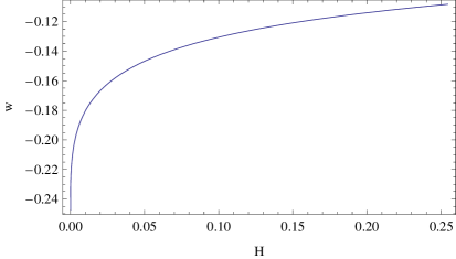
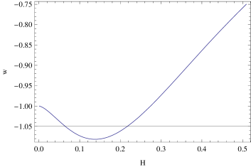
Figure 23: The variation of w𝑤w against H𝐻H for α=2.5,wm=.01,n=.8,ρcard=.1,Λ=.01,ρ0=.001,k=1,l=.9,H0=72formulae-sequence𝛼2.5formulae-sequencesubscript𝑤𝑚.01formulae-sequence𝑛.8formulae-sequencesubscript𝜌𝑐𝑎𝑟𝑑.1formulae-sequenceΛ.01formulae-sequencesubscript𝜌0.001formulae-sequence𝑘1formulae-sequence𝑙.9subscript𝐻072\alpha=2.5,w_{m}=.01,n=.8,\rho_{card}=.1,\Lambda=.01,\rho_{0}=.001,k=1,l=.9,H_{0}=72.
Refer to caption
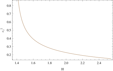
Figure 24: The variation of cs2superscriptsubscript𝑐𝑠2c_{s}^{2} against H𝐻H for α=2.5,wm=.01,n=.8,ρcard=.1,Λ=.01,ρ0=.001,k=1,l=.9,H0=72formulae-sequence𝛼2.5formulae-sequencesubscript𝑤𝑚.01formulae-sequence𝑛.8formulae-sequencesubscript𝜌𝑐𝑎𝑟𝑑.1formulae-sequenceΛ.01formulae-sequencesubscript𝜌0.001formulae-sequence𝑘1formulae-sequence𝑙.9subscript𝐻072\alpha=2.5,w_{m}=.01,n=.8,\rho_{card}=.1,\Lambda=.01,\rho_{0}=.001,k=1,l=.9,H_{0}=72.
Refer to caption
Figure 25: The variation of s𝑠s against r𝑟r for α=2.5,wm=.01,n=.8,ρcard=.1,Λ=.01,ρ0=.001,k=1,l=.9,H0=72formulae-sequence𝛼2.5formulae-sequencesubscript𝑤𝑚.01formulae-sequence𝑛.8formulae-sequencesubscript𝜌𝑐𝑎𝑟𝑑.1formulae-sequenceΛ.01formulae-sequencesubscript𝜌0.001formulae-sequence𝑘1formulae-sequence𝑙.9subscript𝐻072\alpha=2.5,w_{m}=.01,n=.8,\rho_{card}=.1,\Lambda=.01,\rho_{0}=.001,k=1,l=.9,H_{0}=72.
Refer to caption
Figure 26: The variation of q𝑞q against H𝐻H for α=2.5,wm=.01,n=.8,ρcard=.1,Λ=.01,ρ0=.001,k=1,l=.9,H0=72formulae-sequence𝛼2.5formulae-sequencesubscript𝑤𝑚.01formulae-sequence𝑛.8formulae-sequencesubscript𝜌𝑐𝑎𝑟𝑑.1formulae-sequenceΛ.01formulae-sequencesubscript𝜌0.001formulae-sequence𝑘1formulae-sequence𝑙.9subscript𝐻072\alpha=2.5,w_{m}=.01,n=.8,\rho_{card}=.1,\Lambda=.01,\rho_{0}=.001,k=1,l=.9,H_{0}=72.
Refer to caption
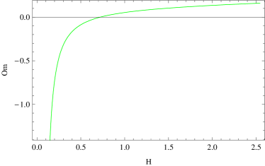
Figure 27: The variation of Om𝑂𝑚Om against H𝐻H for α=2.5,wm=.01,n=.8,ρcard=.1,Λ=.01,ρ0=.001,k=1,l=.9,H0=72formulae-sequence𝛼2.5formulae-sequencesubscript𝑤𝑚.01formulae-sequence𝑛.8formulae-sequencesubscript𝜌𝑐𝑎𝑟𝑑.1formulae-sequenceΛ.01formulae-sequencesubscript𝜌0.001formulae-sequence𝑘1formulae-sequence𝑙.9subscript𝐻072\alpha=2.5,w_{m}=.01,n=.8,\rho_{card}=.1,\Lambda=.01,\rho_{0}=.001,k=1,l=.9,H_{0}=72.

From (16), (18), (19), (20), (47) and (48) we get the statefinder parameters and deceleration parameter,

r=[2(1+z)6wmρcard2+(1+z)33wmρ0ρcard(49(1+nXME)wm(1+wm))+(1+z)6ρ02(2+9wm\displaystyle r=\left[2(1+z)^{-6w_{m}}\rho_{card}^{2}+(1+z)^{3-3w_{m}}\rho_{0}\rho_{card}(4-9(-1+nX_{ME})w_{m}(1+w_{m}))+(1+z)^{6}\rho_{0}^{2}(2+9w_{m}\right.
+9(wm2+n2XME2(1+wm)2+nXME(1+wm)(1+n+(2+n)wm)))]/[2(1+z)3wmρcard2+2(1+z)3ρ0]\left.+9(w_{m}^{2}+n^{2}X_{ME}^{2}(1+w_{m})^{2}+nX_{ME}(1+w_{m})(-1+n+(-2+n)w_{m})))\right]/\left[2(1+z)^{-3w_{m}}\rho_{card}^{2}+2(1+z)^{3}\rho_{0}\right] (51)

and

s=[2(1+z)6wmρcard2+(1+z)33wmρ0ρcard(2+nXME(1+wm)(2+9wm)wm(11+9wm))\displaystyle s=\left[2(1+z)^{-6w_{m}}\rho_{card}^{2}+(1+z)^{3-3w_{m}}\rho_{0}\rho_{card}(2+nX_{ME}(1+w_{m})(2+9w_{m})-w_{m}(11+9w_{m}))\right.
(1+z)6ρ02(9n2XME2(1+wm)2+wm(11+9wm)+nXME(1+wm)(11+9n+9(2+n)wm))]\displaystyle\left.-(1+z)^{6}\rho_{0}^{2}(9n^{2}X_{ME}^{2}(1+w_{m})^{2}+w_{m}(11+9w_{m})+nX_{ME}(1+w_{m})(-11+9n+9(-2+n)w_{m}))\right]
/[(2((1+z)3ρ0+(1+z)3wmρcard)((1+z)3wmρcard+(1+z)3ρ0(wm+nXME(1+wm))))]absentdelimited-[]2superscript1𝑧3subscript𝜌0superscript1𝑧3subscript𝑤𝑚subscript𝜌𝑐𝑎𝑟𝑑superscript1𝑧3subscript𝑤𝑚subscript𝜌𝑐𝑎𝑟𝑑superscript1𝑧3subscript𝜌0subscript𝑤𝑚𝑛subscript𝑋𝑀𝐸1subscript𝑤𝑚/\left[(2((1+z)^{3}\rho_{0}+(1+z)^{-3w_{m}}\rho_{card})((1+z)^{-3w_{m}}\rho_{card}+(1+z)^{3}\rho_{0}(-w_{m}+nX_{ME}(1+w_{m}))))\right] (52)
q=2(1+z)3wmρcard+(1+z)3ρ0(13wm+3nXME(1+wm))2(1+z)3ρ0+2(1+z)3wmρcard𝑞2superscript1𝑧3subscript𝑤𝑚subscript𝜌𝑐𝑎𝑟𝑑superscript1𝑧3subscript𝜌013subscript𝑤𝑚3𝑛subscript𝑋𝑀𝐸1subscript𝑤𝑚2superscript1𝑧3subscript𝜌02superscript1𝑧3subscript𝑤𝑚subscript𝜌𝑐𝑎𝑟𝑑q=-\frac{2(1+z)^{-3w_{m}}\rho_{card}+(1+z)^{3}\rho_{0}(-1-3w_{m}+3nX_{ME}(1+w_{m}))}{2(1+z)^{3}\rho_{0}+2(1+z)^{-3w_{m}}\rho_{card}} (53)

Fig.21, 22 and 23  represents the variation of g𝑔g, wcsubscript𝑤𝑐w_{c} and w𝑤w against H𝐻H respectively. From (9), (10), (16), (47) and (48) we plot the graph which shows the variation of the square of velocity of sound cs2superscriptsubscript𝑐𝑠2c_{s}^{2} against H𝐻H is given in Fig. 24, Fig.25  represents the variation of s𝑠s against r𝑟r and Fig.26  represents the variation of q𝑞q against H𝐻H. From (8), (21) and (46) we get the value of Om. Fig.27  represents the variation of Om𝑂𝑚Om against H𝐻H. The values are taken as, α=2.5,wm=.01,n=.8,ρcard=.1,Λ=.01,ρ0=.001,k=1,l=.9,H0=72formulae-sequence𝛼2.5formulae-sequencesubscript𝑤𝑚.01formulae-sequence𝑛.8formulae-sequencesubscript𝜌𝑐𝑎𝑟𝑑.1formulae-sequenceΛ.01formulae-sequencesubscript𝜌0.001formulae-sequence𝑘1formulae-sequence𝑙.9subscript𝐻072\alpha=2.5,w_{m}=.01,n=.8,\rho_{card}=.1,\Lambda=.01,\rho_{0}=.001,k=1,l=.9,H_{0}=72. From the figures, we see that g,wc,w,q𝑔subscript𝑤𝑐𝑤𝑞g,w_{c},w,q first decrease then increase and Om𝑂𝑚Om decreases as H𝐻H decreases and cs2superscriptsubscript𝑐𝑠2c_{s}^{2} lies between 0 and 1. The parameter s𝑠s increases and keeps positive sign as r𝑟r decreases.

V Discussions

In this work, the we have considered Cardassian Universe in Horˇˇr\check{\text{r}}ava-Lifshitz gravity. The energy density and pressure for Cardassian term have been found. Four types of Cardassian Universe models i.e., polytropic/power law, modified polytropic, exponential and modified exponential models have been considered for accelerating models. To investigate the natures of statefinder parameters, deceleration parameter, Om𝑂𝑚Om diagnostic and EoS parameters for all types of Cardassian models in Horˇˇr\check{\text{r}}ava-Lifshitz gravity, we have drawn all parameters w.r.t. Hubble parameters H𝐻H.

In polytropic/power law Cardassian model of the universe g,w,q𝑔𝑤𝑞g,w,q and Om𝑂𝑚Om parameters have been drawn in figures 1, 2, 5 and 6. We have seen that g,w,q𝑔𝑤𝑞g,w,q and Om𝑂𝑚Om decrease as H𝐻H decreases. The values are taken as, wm=.01,n=.5,ρcard=.1,Λ=.01,ρ0=.001,k=1,l=.9,H0=72formulae-sequencesubscript𝑤𝑚.01formulae-sequence𝑛.5formulae-sequencesubscript𝜌𝑐𝑎𝑟𝑑.1formulae-sequenceΛ.01formulae-sequencesubscript𝜌0.001formulae-sequence𝑘1formulae-sequence𝑙.9subscript𝐻072w_{m}=.01,n=.5,\rho_{card}=.1,\Lambda=.01,\rho_{0}=.001,k=1,l=.9,H_{0}=72. In this model, the EoS parameter wcsubscript𝑤𝑐w_{c} is constant. The variation of the square of velocity of sound cs2superscriptsubscript𝑐𝑠2c_{s}^{2} against H𝐻H is given in fig.3 and it has been observed that cs2superscriptsubscript𝑐𝑠2c_{s}^{2} lies between 0 and 1. Also fig.4 represents the variation of s𝑠s against r𝑟r and the figure shows that s𝑠s increases and keeps positive sign as r𝑟r decreases from positive to negative values.

In modified polytropic Cardassian model of the universe g,wc,w,q𝑔subscript𝑤𝑐𝑤𝑞g,w_{c},w,q and Om𝑂𝑚Om parameters have been drawn in figures 7, 8, 9, 12 and 13. We have seen that g,wc,w,q𝑔subscript𝑤𝑐𝑤𝑞g,w_{c},w,q and Om𝑂𝑚Om decrease as H𝐻H decreases. The values are taken as, α=.5,wm=.01,n=.5,ρcard=.1,Λ=.01,ρ0=.001,k=1,l=.9,H0=72formulae-sequence𝛼.5formulae-sequencesubscript𝑤𝑚.01formulae-sequence𝑛.5formulae-sequencesubscript𝜌𝑐𝑎𝑟𝑑.1formulae-sequenceΛ.01formulae-sequencesubscript𝜌0.001formulae-sequence𝑘1formulae-sequence𝑙.9subscript𝐻072\alpha=.5,w_{m}=.01,n=.5,\rho_{card}=.1,\Lambda=.01,\rho_{0}=.001,k=1,l=.9,H_{0}=72. The variation of the square of velocity of sound cs2superscriptsubscript𝑐𝑠2c_{s}^{2} against H𝐻H is given in fig.10 and it has been observed that cs2superscriptsubscript𝑐𝑠2c_{s}^{2} lies between 0 and 1. Also fig.11 represents the variation of s𝑠s against r𝑟r and the figure shows that s𝑠s increases and keeps positive sign as r𝑟r decreases from positive to negative values.

In exponential Cardassian model of the universe g,wc,w,q𝑔subscript𝑤𝑐𝑤𝑞g,w_{c},w,q and Om𝑂𝑚Om parameters have been drawn in figures 14, 15, 16, 19 and 20. We have seen that g,wc,w,q𝑔subscript𝑤𝑐𝑤𝑞g,w_{c},w,q and Om𝑂𝑚Om decrease as H𝐻H decreases. The values are taken as, wm=.01,n=2,ρcard=.1,Λ=.01,ρ0=.001,k=1,l=.9,H0=72formulae-sequencesubscript𝑤𝑚.01formulae-sequence𝑛2formulae-sequencesubscript𝜌𝑐𝑎𝑟𝑑.1formulae-sequenceΛ.01formulae-sequencesubscript𝜌0.001formulae-sequence𝑘1formulae-sequence𝑙.9subscript𝐻072w_{m}=.01,n=2,\rho_{card}=.1,\Lambda=.01,\rho_{0}=.001,k=1,l=.9,H_{0}=72. The variation of the square of velocity of sound cs2superscriptsubscript𝑐𝑠2c_{s}^{2} against H𝐻H is given in fig.17 and it has been observed that cs2superscriptsubscript𝑐𝑠2c_{s}^{2} lies between 0 and 1. Also fig.18 represents the variation of s𝑠s against r𝑟r and the figure shows that s𝑠s increases and keeps negative sign as r𝑟r decreases.

In modified exponential Cardassian model of the universe g,wc,w,q𝑔subscript𝑤𝑐𝑤𝑞g,w_{c},w,q and Om𝑂𝑚Om parameters have been drawn in figures 21, 22, 23, 26 and 27. We have seen that g,wc,w,q𝑔subscript𝑤𝑐𝑤𝑞g,w_{c},w,q first decrease then increase and Om𝑂𝑚Om decreases as H𝐻H decreases. The values are taken as, α=2.5,wm=.01,n=.8,ρcard=.1,Λ=.01,ρ0=.001,k=1,l=.9,H0=72formulae-sequence𝛼2.5formulae-sequencesubscript𝑤𝑚.01formulae-sequence𝑛.8formulae-sequencesubscript𝜌𝑐𝑎𝑟𝑑.1formulae-sequenceΛ.01formulae-sequencesubscript𝜌0.001formulae-sequence𝑘1formulae-sequence𝑙.9subscript𝐻072\alpha=2.5,w_{m}=.01,n=.8,\rho_{card}=.1,\Lambda=.01,\rho_{0}=.001,k=1,l=.9,H_{0}=72. The variation of the square of velocity of sound cs2superscriptsubscript𝑐𝑠2c_{s}^{2} against H𝐻H is given in fig.24 and it has been observed that cs2superscriptsubscript𝑐𝑠2c_{s}^{2} lies between 0 and 1. Also fig.25 represents the variation of s𝑠s against r𝑟r and the figure shows that s𝑠s increases and keeps positive sign as r𝑟r decreases.

Acknowledgement:

The authors are thankful to IUCAA, Pune, India for warm hospitality where part of the work was carried out.

References:

[1]delimited-[]1[1]
A. Riess, et al., Astron. J. 116 (1998) 1009.
[2]delimited-[]2[2] S. J. Perlmutter, et al., Astrophys. J. 517 (1999) 565.
[3]delimited-[]3[3] J. L. Tonry, et al., Astrophys. J. 594 (2003) 1.
[4]delimited-[]4[4] B. Barris, et al., Astrophys. J. 602 (2004) 571.
[5]delimited-[]5[5] R. Knop, et al., Astrophys. J. 598 (2003) 102.
[6]delimited-[]6[6] A.G. Riess, et al., Astrophys. J. 607 (2004) 665.
[7]delimited-[]7[7] P. Astier, et al., Astron. Astrophys. 447 (2006) 31.
[8]delimited-[]8[8] P. J. Steinhardt, L. Wang and I. Zlater, Phys. Rev. D 59(1999) 123504.
[9]delimited-[]9[9] X. Z. Li, J. G. Hao and D. J. Liu, Class. Quant. Grav. 19 (2002) 6049.
[10]delimited-[]10[10] D. J. Liu and X. Z. Li, Phys. Lett. B 611 (2005) 8.
[11]delimited-[]11[11] K. Freese, F.C. Adams, J.A. Frieman, and E. Mottola, Nucl. Phys. B287, 797(1987).
[12]delimited-[]12[12] P.J.E. Peebles and B. Ratra, Astrophys. J., Lett. Ed. 325, L17(1988).
[13]delimited-[]13[13] B. Ratra and P.J.E. Peebles, Phys. Rev. D 37, 3406(1988).
[14]delimited-[]14[14] J. Frieman, C. Hill, A. Stebbins, and I. Waga, Phys. Rev. Lett. 75, 2077(1995).
[15]delimited-[]15[15] L. Wang and P. Steinhardt, Astrophys. J. 508, 483(1998).
[16]delimited-[]16[16] R. Caldwell, R. Dave, and P. Steinhardt, Phys. Rev. Lett. 80, 1582(1998).
[17]delimited-[]17[17] G. Huey, L. Wang, R. Dave, R. Caldwell, and P. Steinhardt, Phys. Rev. D 59, 063005(1999).
[18]delimited-[]18[18] C. Deffayet, Phys. Lett. B 502, 199(2001).
[19]delimited-[]19[19] C. Deffayet, G. Dvali, and G. Gabadadze, Phys. Rev. D 65, 044023(2002).
[20]delimited-[]20[20] C.B. Netterfield et al, Astrophys. J. 571 (2002) 604.
[21]delimited-[]21[21] R. Stompor et al, Astrophys. J. 561 (2001) L7.
[22]delimited-[]22[22] K. Freese, M. Lewis, Phys. Lett. B 540 (2002)1.
[23]delimited-[]23[23] K. Freese, New Astron. Rev. 49 (2005) 103; Nucl. Phys. (Proc. Suppl.) 124 50 (2003).
[24]delimited-[]24[24] R. Lazkoz, G. Le n, Phys. Rev. D 71 (2005) 123516.
[25]delimited-[]25[25] Y. Wang, K. Freese, P. Gondolo, M. Lewis, Astrophys. J. 594(2003) 25.
[26]delimited-[]26[26] D. J. Liu, C. B. Sun and X. Z. Li, Phys. Lett. B 634, 442 (2006).
[27]delimited-[]27[27] C. Pryke et al, Astrophys. J. 568, 46 (2002); N.W. Halverson et al, Astrophys. J. 568 (2002) 38.
[28]delimited-[]28[28] P. Horˇˇr\check{\text{r}}ava, JHEP 0903 020 (2009).
[29]delimited-[]29[29] P. Horˇˇr\check{\text{r}}ava, Phys. Rev. D 79 084008 (2009).
[30]delimited-[]30[30] E. M. Lifshitz, Zh. Eksp. Teor. Fiz. 11 255 (1949).
[31]delimited-[]31[31] R. G. Cai et al, Phys. Rev. D 80 041501 (2009).
[32]delimited-[]32[32] G. Calcagni, JHEP 0909 112 (2009).
[33]delimited-[]33[33] H. Lu et al, Phys. Rev. Lett. 103 091301 (2009).
[34]delimited-[]34[34] V. Sahni, T. D. Saini, A. A. Starobinsky, and U. Alam, JETP Lett. 77, 201 (2003).
[35]delimited-[]35[35] V. Sahni, A. Shafieloo and A. A. Starobinsky, Phys. Rev. D 78, 103502 (2008).
[36]delimited-[]36[36] J. Lu, L. Xu, Y. Gui and B. Chang, arXiv:0812.2074v2 [astro-ph];
[37]delimited-[]37[37] R. L. Arnowitt, S. Deser and C. W. Misner, The Dynamics of General Relativity appeared as Chapter 7, pp. 227-264, in gravitation: an introduction to current research, L. Witten, ed. (Wiley, New York, 1962), arXiv: gr-qc/0405109.
[38]delimited-[]38[38] C. Charmousis, G. Niz, A. Padilla and P. M. Saffin, JHEP 0908 070 (2009); T. P. Sotiriou, M. Visser and S. Weinfurtner, JHEP 0910 (2009) 033; C. Bogdanos and E. N. Saridakis, Class. Quant. Grav. 27 075005 (2010).