Degradation modeling applied to residual lifetime prediction using functional data analysis
Abstract
Sensor-based degradation signals measure the accumulation of damage of an engineering system using sensor technology. Degradation signals can be used to estimate, for example, the distribution of the remaining life of partially degraded systems and/or their components. In this paper we present a nonparametric degradation modeling framework for making inference on the evolution of degradation signals that are observed sparsely or over short intervals of times. Furthermore, an empirical Bayes approach is used to update the stochastic parameters of the degradation model in real-time using training degradation signals for online monitoring of components operating in the field. The primary application of this Bayesian framework is updating the residual lifetime up to a degradation threshold of partially degraded components. We validate our degradation modeling approach using a real-world crack growth data set as well as a case study of simulated degradation signals.
doi:
10.1214/10-AOAS448keywords:
., and m1Supported in part by the NSF Grant CMMI-0738647.
1 Introduction
Most failures of engineering systems result from a gradual and irreversible accumulation of damage that occurs during a system’s life cycle. This process is known as degradation [Bogdanoff and Kozin (1985)]. In many applications, it can be very difficult to assess and observe physical degradation, especially when real-time observations are required. However, degradation processes are almost always associated with some manifestations that are much easier to observe and monitor overtime. Generally, the evolution of these manifestations can be monitored using sensor technology through a process known as Condition Monitoring (CM). The observed condition-based signals are known as degradation signals [Nelson (1990)] and are usually correlated with the underlying physical degradation process. Some examples of degradation signals include vibration signals for monitoring excessive wear in rotating machinery, acoustic emissions for monitoring crack propagation, temperature changes and oil debris for monitoring engine lubrication and many others.
Degradation modeling attempts to characterize the evolution of degradation signals. There is a significant number of research works that have focused on degradation models; these include models presented in Lu and Meeker (1993), Padgett and Tomlinson (2004), Gebraeel et al. (2005), Müller and Zhang (2005), Gebraeel (2006) and Park and Padgett (2006). Many of these models rely on a representative sample of complete degradation signals. A complete degradation signal is a continuously observed signal that captures the degradation process of a component from a brand “New State” to a completely “Failed State.”
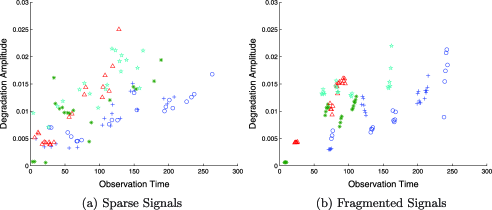
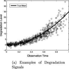
Unfortunately, building a database of complete degradation signals can be very expensive and time consuming in applications, such as monitoring of jet engines, turbines, power generating units, structures and bridges and many others. For example, in applications consisting of relatively static structures such as bridges, degradation usually takes place very slowly (several tens of years). Since the system is relatively static, it suffices to observe the degradation process at intermittent discrete time points. The result is a sparsely observed degradation signal such as the signals depicted in Figure 1(a). In contrast, in applications consisting of dynamic systems, such as turbines, generators and machines, degradation cannot be reasonably assessed by sparse measurements. At the same time, continuous observations of the complete degradation process of such systems are economically unjustifiable. Usually, the only way to gain a relatively accurate understanding of the health/performance of a dynamic system is to monitor its performance over a time interval. In naval maritime applications, power generating units of an aircraft are removed, tested for a short period of time (during which degradation data can be acquired) and put back into operation. The result is a collection of fragmented degradation signals as depicted in Figure 1(b).
In this paper we develop a degradation model that applies to incomplete degradation signals as well as complete degradation signals. An incomplete degradation signal is defined as a signal that consists of sparse observations of the degradation process or continuous observations made over short time intervals (fragments). One challenge in such applications is that the evolution of the degradation signals cannot be readily assessed to determine the parametric form of the underlying degradation model. This is because one cannot clearly trace how a degradation signal progresses over time from incomplete observations. For example, is there a well defined parametric model that describes the signals in Figure 1?
To overcome this challenge, the underlying degradation model in this paper is assumed nonparametric. Most degradation models used to characterize the evolution of sensor-based degradation signals are parametric models. A common approach is to model the degradation signals using a parametric (linear) model with random coefficients [Lu and Meeker (1993); Gebraeel et al. (2005); Gebraeel (2006)]. Other modeling approaches assume that the degradation signal follows a Brownian motion process [Doksum and Hoyland (1992); Pettit and Young (1999)] or a Gaussian process with known covariance structure [Padgett and Tomlinson (2004); Park and Padgett (2006)]. In contrast, we assume that the mean and covariance functions of the degradation process are unknown and they are estimated based on an assembly of training incomplete degradation signals. The mean function is estimated using standard nonparametric regression methods such as local smoothing [Fan and Yao (2003)]. The covariance function is decomposed using the Karhunen–Loève decomposition [Karhunen (1947); Loève (1945)] and estimated using the Functional Principal Component Analysis (FPCA) method introduced by Yao, Müller and Wang (2005).
Under the nonparametric modeling framework, one condition for accurate estimation of the mean and covariance functions is that the degradation process is densely observed throughout its support. However, in applications where the degradation signals are incompletely sampled, not all degradation signals are observed up to the point of failure; in addition, only a few components will survive up to the maximum time point of the degradation process support. Consequently, the degradation process is commonly under-sampled close to the upper bound of its support. To overcome this difficulty, we introduce a nonuniform sampling procedure for collecting incomplete degradation signals, which ensures relatively dense coverage throughout the sampling time domain.
One important application of degradation modeling is predicting the lifetime of components operating in the field. For real-time monitoring, an empirical Bayes approach is introduced to update the stochastic parameters of the degradation model. In this paper we focus on estimation of the distribution of the residual life up to a degradation threshold for partially degraded components using training degradation signals which are sparsely or completely observed. Other applications of the degradation modeling and the Bayesian updating procedure are estimation of the lifetime at a specified degradation level and estimation of the degradation level at a specified lifetime.
We evaluate the performance of our methodology using both a crack growth data set and simulated degradation signals. In these empirical studies we compare parametric to nonparametric degradation modeling, assess the estimation accuracy of the remaining lifetime for complete and incomplete signals, and contrast uniform vs. nonuniform sampling procedures for acquiring ensembles of incomplete degradation signals. In both studies there is not a significant decrease in the accuracy of the residual life estimation when using ensembles of incomplete instead of complete signals. We also highlight the robustness of our approach by comparing it with misspecified parametric models, which are common when the underlying degradation process is complicated and sparsely observed. Last, we show in the simulation study that using a nonuniform sampling procedure that ensures dense observation of the sampling time domain reduces the estimation error. Based on these empirical studies, we conclude that the nonparametric approach introduced in this paper is efficient in characterizing the underlying degradation process and it is more robust to model misspecification than parametric approaches, which is particularly important when the training signals are incompletely observed (sparse or fragmented).
The remainder of the paper is organized as follows. Section 2 discusses the development of our degradation modeling framework. The empirical Bayes approach for updating the degradation distribution of a partially degraded component is introduced in Section 3. The derivation of the remaining lifetime distribution under the empirical Bayes approach is presented in Section 4. In Section 5 we introduce an experimental design for sampling incomplete degradation signals. We discuss performance results of our methodology using real-world and simulated degradation signals in Section 6 and 7, respectively.
2 Sensor-based degradation modeling
We denote the observed degradation signals , for ( is the number of observation time points for signal ) and ( is the number of signals) where are the observation time points in a bounded time domain for signal . Note that will always be finite since any industrial application has a finite time of failure. We model the distribution of the signals by borrowing information across multiple degradation signals. We decompose the degradation signal as
| (1) |
where is the underlying trend of the degradation process and is assumed to be fixed but unknown, and represents the random deviation from the underlying degradation trend. We also assume and are independent.
The model in (1) is a general decomposition for functional data with various modeling alternatives and assumptions for the model components: , , and . In this paper we discuss one such modeling alternative which applies to sparse and fragmented signals as well as to complete signals and it applies under the assumption that the observation time points are fixed but not necessarily equally spaced and the assumption that the error terms are independent and identically distributed. Deviations from these assumptions may require some modifications to the modeling approach discussed in this paper.
In our modeling approach, the degradation signal follows a stochastic process with mean and stochastic deviations with mean zero and covariance . The mean function and the covariance surface are both assumed to be nonparametric, that is, no prespecified assumption on their shape. This generalized assumption encompasses the particular cases developed earlier by Gebraeel et al. (2005) and Gebraeel (2006), which assume a linear trend, where and , and parametric covariance structure .
The following steps discuss how we estimate the mean function and the covariance surface of our degradation model. {longlist}[Step 1:]
We use nonparametric methods to estimate the mean . In this paper we use local quadratic smoothing [Fan and Yao (2003)] to allow estimation of the mean function under general settings including complete and incomplete (sparse and fragmented) signals. The bandwidth parameter, which controls the smoothing level, is selected using the leave-one-curve-out cross-validation method [Rice and Silverman (1991)]. Alternative estimation methods include decomposition of the mean function using a basis of functions (e.g., splines, Fourier, wavelets) and estimate the coefficients using parametric methods. These alternative methods will apply under various signal behaviors (e.g., smooth vs. with sharp changes, uniformly vs. nonuniformly sampled).
The covariance surface is estimated using the demeaned data, , where is the local quadratic smoothing estimate of . Using the Karhunen–Loéve decomposition [Karhunen (1947); Loève (1945)], the covariance, , can be expressed as follows:
| (2) |
where for are the associated eigenfunctions with support and are the ordered eigenvalues. Based on this decomposition, the deviations from the underlying degradation trend are decomposed using the following expression:
| (3) |
where called scores are uncorrelated random effects with mean zero and variance . The decomposition in equation (3) is an infinite sum. Generally, only a small number of eigenvalues are commonly significantly nonzero. For the eigenvalues which are approximately zero, the corresponding scores will also be approximately zero. Consequently, we use a truncated version of this decomposition. Therefore, expression (3) can be approximated as follows:
| (4) |
where is the number of significantly nonzero eigenvalues. We select to minimize the modified Akaike criterion defined by Yao, Müller and Wang (2005).
In the statistical literature this method has been coined Functional Principal Component Analysis (FPCA). The key reference for FPCA is Ramsay and Silverman [(1997), Chapter 8]. Another important reference is Yao, Müller and Wang (2005), in which the authors derived theoretical results for model parameter consistency and asymptotic ( large) distribution results under the assumption that the scores follow a normal distribution.
An alternative method for estimating the covariance function of the process is decomposing the covariance function as in equation (2) where the basis of functions is fixed [James, Hastie and Sugar (2000)]. However, this approach doesn’t allow dimensionality reduction in the same way FPCA does and it is not theoretically founded.
3 Degradation model updating
Next, we consider a component operating in the field called fielded component. Assume that we have observed its degradation signal at a vector of time ; therefore, denotes the observed signal of the testing component, represents the number of observations and denotes the latest observation time. In this section we introduce an Empirical Bayes approach which allows real-time updating of the distribution of the degradation process for partially degraded components given the observed signal and the prior distribution of the scores for The prior distribution of the scores is estimated empirically from a set of historical degradation signals.
Proposition 1 illustrates the updating procedure assuming that the prior distribution of the scores is normal and assuming that the mean function and the basis of functions , , are fixed. The proof of this proposition follows from the theory of Bayesian linear models.
Proposition 1
Assume that follows
where the prior distribution of is with uncorrelated; are independent of for ; the distribution of is with fixed. It follows that the posterior distribution of the scores is
where
with
In Proposition 1 the prior distribution of the scores is specified by the variance parameters , , which are estimated using the degradation model in Section 2 and based on a set of incomplete or complete training degradation signals. Specifically, we first apply Functional Principal Component Analysis on the historical degradation signals which will further provide estimates for the variance parameters , , and the eigenfunctions , . Based on these estimates, we obtain the posterior distributions of the updated scores since the matrix and the vector are fully determined by the eigenvalues , , and the eigenfunctions , . The expectation of the posterior scores is nonzero and, therefore, we denote the posterior mean function .
Following Proposition 1, the expectation of the posterior distribution follows the same formula as the conditional expectation estimator in Yao, Müller and Wang (2005), equation (4). Generally, this similarity applies under the empirical Bayesian prior derived from FPCA. On the other hand, the sampling distribution of the conditional expectation estimator in Yao, Müller and Wang (2005) is different from the posterior distribution of , since their variances are not equal. Moreover, the conditional expectation estimator and its mean estimation error in Yao, Müller and Wang (2005) are conditional on the training observations, whereas the posterior distribution in Proposition 1 is conditional on the observations of a new component.
The advantage of this Bayesian framework is that it unifies the conditional expectation estimation and prediction into a procedure which allows updating the distribution of the degradation process for a new component. We can therefore use the posterior distribution of the scores for a partially degraded signal to estimate the distribution of various statistical summaries, including the lifetime at a specified degradation level and estimation of the degradation level at a specified time. In the next section we discuss one specific application to this updating framework: residual life estimation.
4 Remaining life distribution
In this paper we focus our attention on engineering applications where a soft-failure of a system occurs once its underlying degradation process reaches a predetermined critical threshold. This critical threshold is commonly used to initiate maintenance activities such as repair and/or component replacement well in advance of catastrophic failure. Consequently, degradation data can still be observed beyond the critical threshold. In this section we describe how our degradation modeling framework is applied to estimate the distribution of remaining life up to a degradation threshold of partially degraded systems.
In the remainder of this section, will denote the underlying degradation process of a partially degraded system. Based on the degradation process , the failure time of a system is defined as
| (6) |
One has to bear in mind that may not exist if the threshold is set too high, that is, the component may fail before its degradation signal reaches the threshold. The selection of the failure threshold is an important problem, however, this aspect is beyond the scope of this paper. In this work, we assume that exists, and the threshold is known a priori. This is a reasonable assumption because in many industrial applications failure/alarm thresholds are usually based on subjective engineering judgement or well-accepted standards, such as the International Standards Organization (ISO) (e.g., the ISO 2372 is used for defining acceptable vibration threshold levels for different machine classifications). A second assumption is that the failure time is smaller than a maximum failure time . This assumption is also reasonable, as in practice a component may be replaced after a given period of time even if it did not fail.
The distribution of the residual life (RLD) of a partially degraded component at a fixed time is estimated assuming that the degradation process of the component follows a posterior distribution based on Proposition 1. We estimate the distribution of the residual life (RLD) using
where and are the posterior mean and covariance functions of the degradation process . The derivations of and are based on the results of Proposition 1. We note here that the distribution of the RLD above is not conditional on the observed signal of the partially degraded component but on the posterior distribution of its degradation process; since the degradation is only partially observed and most often sparsely sampled, conditioning on the posterior distribution will generally provide a more accurate RLD estimator since we incorporate the additional information in the training degradation signals.
Furthermore, we estimate RLD under two assumptions:
-
[A.0]
-
A.1
The new component has not failed up to the last observation time point , that is, the failure time becomes
-
A.2
We assume the probability that the degradation process crosses back the threshold after the failure time is negligible, that is, for all . This implies, if we condition on , which is the same as conditioning on , . This further implies
Under these two assumptions, the RLD becomes
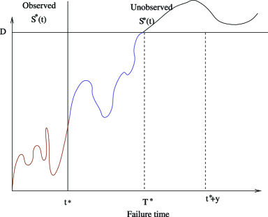
The approximation in assumption A.2 is similar to the approximation in the paper by Lu and Meeker (1993) which assumes that the probability of a negative random slope in the linear model is negligible. One particular case for the assumption A.2 to hold is that the signal is monotone. However, monotonicity is not a necessary condition. Assumption A.2 also holds for nonmonotone signals—an example of such a signal is in Figure 2.
Proposition 2 below describes the updating procedure for RLD of a new component given the posterior distribution of its degradation process updated up to time . The proof follows directly as a consequence of Proposition 1.
Proposition 2
For a new partially degraded component with its degradation process updated up to time , the residual life distribution is given as follows:
| (7) |
where represents the standard normal cumulative distribution function and with
In the above equations, , and refers to the element of the matrix .
One advantage of obtaining the distribution rather than simply a point estimate is that we can also derive a confidence interval for the remaining lifetime up to a degradation threshold . Following the derivation in Proposition 2, a confidence interval for RLD is such that
Since we have one equation with two unknowns, the lower— and the upper— tails are commonly equally weighted, and, therefore,
and
However, we cannot obtain exact solutions for and because we do not have a closed-form expression for the inverse of the cumulative density function of . For example, the first relationship is equivalent to finding from where is the quantile of the normal distribution. Using this equation, we would like to obtain such that
which is a nonlinear function of and its solution does not have a close form expression. We therefore resort to parametric bootstrap [Efron and Tibshirani (1993); Davison and Hinkley (1997)] to sample from the distribution of which will give us a set of realizations from this distribution—. Using these realizations from the distribution of , we estimate a quantile bootstrap confidence interval.
The confidence interval estimation procedure is as follows. For :
-
1.
Sample from the multivariate normal distribution of the posterior scores provided in Proposition 1.
-
2.
Obtain a simulated signal
where , , are the scores sampled at Step 1.
-
3.
Take .
Using the sampled values , we compute the empirical and quantiles, and , respectively. We estimate the upper and lower bound of the confidence interval by and . It follows that is an approximate quantile bootstrap confidence interval for the residual life time of the fielded component.
An additional approach to the (parametric) bootstrap method described above is to (re)sample the signal data resulting in multiple bootstrap samples. For each bootstrap sample, estimate the residual lifetime using the approach discussed in this paper; therefore, we obtain a set of realization from the distribution of . In contrast to the bootstrap method described above, this alternative bootstrap approach requires estimating the FPCA model for each bootstrap sample which is computationally expensive.
5 Sampling scheme
The nonparametric degradation modeling framework introduced in this paper applies to both complete as well as incomplete degradation signals. For applications involving incomplete degradation signals, it is important to develop a sampling plan that ensures accurate estimation of the mean function and the covariance surface. Yao, Müller and Wang (2005) provide theoretical results on the estimation of the covariance surface using FPCA under large but small for . In other words, for these results to hold, the observation time points need to cover the time domain, , densely.
Using the traditional uniform sampling technique, the number of observations per time interval decreases as more signals fail, leading to an unbalanced number of observations per time interval—more observations at the beginning of the observation time domain but fewer observations at the end of the time domain. Further, this unbalanced design will result in decreasing estimation accuracy (higher variances) of the mean and covariance estimates at later time points. In order to balance the number of observations per time interval throughout the time domain , we propose an experimental design using nonuniform sampling. The proposed technique ensures relatively dense coverage of the sampling time domain, , where represents the last observation time of the longest possible degradation signal for a given application.
We note here that the sampling technique requires input of at the beginning of the experiment although is unknown. It is often the case that, in practice, an experimenter will set a timeline at the beginning of the experiment which will specify a limit of how long the experiment will be run (e.g., one year vs. one month). This upper limit will specify . Generally, starting with a lower initial value for will allow the experimenter to sample densely enough while having the option to update the sampling technique (update ) if not all training signals have reached the failure threshold by the initial value for .
The following steps outline a sampling procedure for obtaining sparsely observed and fragmented degradation signals: {longlist}[Step 1:]
We begin by performing nonuniform sampling of the time domain , thus obtaining a sequence of time points, , for large . Since only a few components will survive up to the maximum time point, , we increase the sampling frequency at later time points in order to cover the sampling time domain at the extreme point, . Consequently, we sample exponentially, that is, the time interval between two consecutive sampling time points decreases exponentially over time (the decreasing rate is implicitly determined by the value of and the number of sampling time points).
This step provides a potential sampling timetable (or monitoring/observation schedule) for sparsely observed and fragmented degradation signals. We begin by selecting components. For each component, we select its sampling time points from the set without any prior knowledge about their degradation process and lifetime. Next we define two settings: {longlist}[Setting 1:]
This setting is used to obtain sparsely observed degradation signals. For component , we randomly sample time points from the set of total time points . This results in a set of sparse sampling time points, for this component.
This setting is used to obtain fragmented degradation signals. Recall that fragmented signals are obtained by continuously monitoring a component over a short time interval, hence the term “fragment.” For component , we select two or more time points from the set of total time points . These points represent the beginning times of the signal fragments or sampling intervals. The duration of the sampling interval will depend on the type of application, the availability of monitoring/testing equipment and the associated costs/economics. Consequently, the end time points, will vary from one experiment to another. In other words, for component , we may have two or more time intervals: ,
Finally, we observe the degradation signal for the selected components at the selected time points according to the type of incomplete signals, sparse or fragmented, and obtain the set of sampled signals for and .
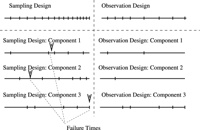
It is important to stress that we select the sampling time points in Step 2 before observing the degradation signals. Since we do not observe the failure time before selecting the time points, we cannot ensure that the degradation signal will be observed for all selected sampling time points. This is because some components may fail before the latest selected time point. Consequently, the observation time points are a subset of the sampling time points and will be less densely sampled close to since the missing observations (the difference set between sampling and observation time points) will increase in density closer to the upper bound . In Figure 3 we compare the sampling time points selected at Step 2 to the observation time points for three components. In this example the sampling time points are nonuniformly selected, whereas the observation time points are approximately uniform since for the first two components, we do not observe at the latest times—only the third component fails after its latest sampling time.
Two parameters that are used for tuning the sampling plan are as follows: the total number of sampling time points and the total number of components . The more sparsely the signals are observed ( is small), the more signals we need to observe ( needs to be large). Selecting and optimally is important to ensure accurate modeling of the degradation process at a feasible cost. The larger the number of components and/or the larger the number of time points are the higher the costs associated with monitoring and testing. Note that selection of and will vary according to the type of application.
6 Case study: Crack growth data
In this section we study crack growth data that can be found in various domains of engineering applications, such as infrastructure (bridges, steel structures), maritime (hulls of oil tankers), aeronautical (aircraft fuselage), energy (vanes of gas turbines), etc. We consider a situation in which crack growth data can be observed from identical units (say, several ship hulls, or turbines) up to a predetermined time period, denoted by in this paper. A constant threshold, , is a critical crack length representing a soft failure when maintenance and repair should be performed. Within this context, we assume that catastrophic failure, that is, hard failure, may occur at a relatively larger crack length.
The data set used in our case study was first published in Virkler, Hillberry and Goel (1979), and has been previously analyzed in other journal articles [Kotulski (1998); Cross, Makeev and Armanios (2006) and the references therein]. The specimens in the test were 2.54-mm-thick and 152.4-mm-wide center cracked sheets of 2024-T3 aluminum. The crack propagation signals of these specimens were recorded under identical experimental conditions. In this data set, the crack length was measured in millimeters and the observation time was measured by the cumulative load cycles. More details about this data set can be found in Virkler, Hillberry and Goel (1979). In this study, we set the soft failure threshold to mm. We provide additional results for another soft threshold in the supplemental material [Zhou, Serban and Gebraeel (2010)]. To be consistent with the methodology in this study, the observations are censored at common value cycles. A representative example of sparsely sampled degradation signals is in Figure 4(a).
6.1 Results and analysis
We report the prediction accuracy of the remaining life for varying time points defining the latest observation time of a partially degraded component. We consider the following degradation percentiles: 10% (the signal has been observed up to time , which equals to 10% of the lifetime), 20%, …, 80% and 90%. For each crack, we predict the updated residual lifetime at each of the nine percentiles using the degradation signal observed up to that respective percentile. The number of signals in this study is 59. We randomly select 50 of the total signals as training signals for estimating the model components, and the rest are validation signals for evaluating the performance of our model in predicting residual life. For each validation signal, we use the following error criteria to assess the prediction accuracy:
| (8) |
We replicate the above procedure for 100 times, and report the distribution of the errors across the 100 simulations using a set of boxplots, each boxplot corresponding to a degradation percentile for the testing components and providing the absolute prediction errors for that percentile.
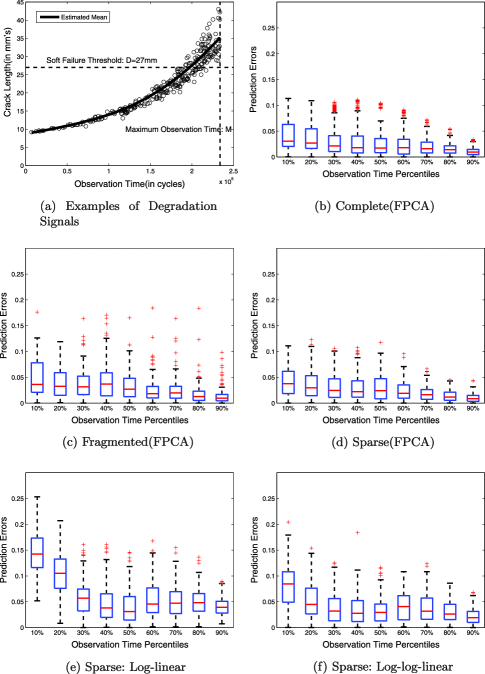
We first discuss the performance of our nonparametric model for complete, sparse and fragmented degradation signals. In each complete degradation signal, we have about 50 observations per signal. To obtain a sparsely observed degradation signal, we randomly sample observations from each complete signal. We use two intervals per signal to obtain fragmented degradation signals. The results are illustrated in Figure 4(b)–(d). The results indicate that our nonparametric model performs well for complete as well as incomplete degradation signals, and the performance is better when the incomplete degradation signals are sparse rather than fragmented. Although we have only approximately observations of complete degradation signals under the sparse sampling scenario, the prediction errors do not increase significantly. This observation is important in practice; under budget limitations, one may resort to sparse or fragmented degradation signals without significant loss of predictive capability.
We also demonstrate the benefits of our proposed nonparametric degradation model by comparing it with parametric models as benchmarks. Since the degradation signals have a nonlinear trend with a curvature similar to the exponential function, we transform the degradation signals using the natural logarithm in order to linearize the trend and then apply a linear random effects model (henceforth, denoted by “log-linear”). Since under the log-transform model, the residual life predictions are inaccurate compared to the nonparametric approach, we consider a double logarithm transformation of the degradation data (henceforth, denoted by “log–log-linear”). The results of the sparse scenario using the parametric models “log-linear” and “log–log-linear” are reported in Figure 4(e)–(f), respectively. We find that both parametric models provide less accurate predictions of the residual life than our nonparametric model. This is due to the inaccuracy of the parametric models in capturing the crack propagation trend.
We provide one example in Figure 5 to illustrate the source of the bias of the “log-linear” model. In this figure the -axis represents the degradation time and the -axis represents the crack length, but in the log scale. We have one complete, sparse and fragmented degradation signal in Figure 5(a)–(c), respectively. If the “log-linear” model is the true underlying parametric model, we should see a linear trend in all three plots. This seems to be true in the sparse or fragmented cases [see Figure 5(b)–(c)]. However, for Figure 5(a) showing a complete signal, we note that the degradation trend is still nonlinear; the log-transformation does not linearize the signal (the same applies for the “log–log” transformation). Therefore, the “log-linear” model does not accurately capture the crack propagation trend throughout the unit’s lifetime. This example shows the potential difficulty of identifying a reasonable parametric model for sparse and fragmented degradation signals and, in turn, demonstrates the robustness of our proposed nonparametric model to model misspecification.

7 Simulation study
In this section we simulate nonlinear degradation signals from three different models to demonstrate the benefits of using our proposed nonparametric degradation modeling approach. We evaluate our approach in terms of the prediction accuracy of estimating the residual life for complete, sparse and fragmented degradation signals, contrast uniform and nonuniform sampling procedures for acquiring the ensembles of incomplete degradation signals, and also investigate the robustness of our model to violations of its model assumptions.
7.1 Simulation models
The degradation signals are simulated from three different models, and all of them are special cases of the general model (1). More specifically:
-
•
In Model 1, we choose , , where , , , and .
-
•
In Model 2, we choose , , where , , and , , . (The coefficients of the eigenfunctions are chosen so that they form an orthonormal functional basis for .)
-
•
In Model 3, we choose , , where , , and , , .
We simulate from Model 1 because its residual life distribution can be easily derived from training signals and updated using validation signals using the procedure in Gebraeel et al. (2005). The derived residual life distribution can then be utilized as a benchmark to assess the performance of our nonparametric approach.
Across all the models, the failure threshold is set to . We generate “training” signals and “validation” signals from each model. For a complete signal, we have 51 observations made at an equally spaced grid on with . A sparse or fragmented signal is then sampled from a complete signal such that we observe about 6 observations per signal. The stopping time for each training signal (the last point at which a signal is observed) is generated from Uniform distribution []—our simulation results are insensitive to the selection of the stopping time distribution.
We run simulations for times. For each simulation, we compute the prediction errors at the following degradation percentiles: 10%, 20%, …, 70%, 80% and 90% of the simulated degradation signals.
 |
 |
 |
 |
 |
 |
 |
 |
|
|
7.1.1 Results and analysis of Model 1
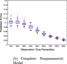
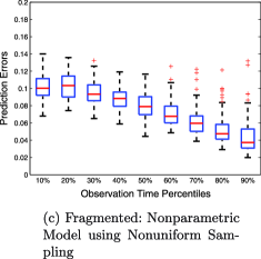
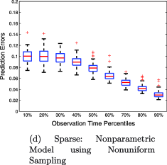
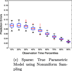
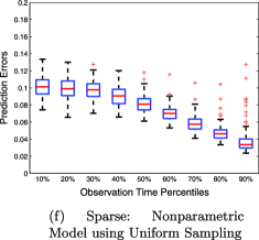
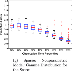
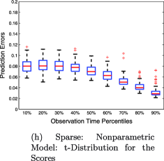
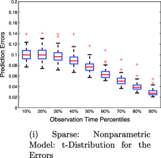
In Figure 6(b)–(d), we present the boxplots of the prediction errors when using the nonparametric degradation model in this paper for complete, fragmented and sparse degradation signals. For the sparse scenario, we compare the prediction accuracy of using the true parametric model [see Figure 6(e)] and our nonparametric model when signals are uniformly sampled [see Figure 6(f)] or nonuniformly sampled [see Figure 6(d)]. We assess the robustness to model assumptions by simulating signals from the model with following a Gamma or Student distribution [see Figure 6(g)–(h)]. We also compute the prediction errors under different error distributions [see Figure 6(i)].
The first observation is that there is insignificant difference in the prediction errors between the true parametric model and the nonparametric degradation model. The differences are larger for high degradation percentiles. Since the difference in the prediction errors increases with additional data, we observe for a new component, we infer that this small inefficiency arises due to a decreased accuracy in the estimation of the empirical prior distribution at the later time points.
The second important observation is that the nonuniform sampling technique proposed in Section 5 enhances the prediction accuracy of the residual life. In Table 1 we list the median prediction errors based on nonuniform sampling and uniform sampling techniques. The first row of this table represents the time percentile of the degradation signals used for predicting the residual life. It is apparent that the nonuniform sampling technique provides smaller prediction errors, especially at high time percentiles. This is because nonuniform sampling ensures dense coverage of observations over the whole time domain, including the region near maximum observation time (), and hence provides more accurate estimate of the mean and covariance functions of the model, especially at higher time percentiles.
| Time percentiles | 20% | 30% | 40% | 50% | 60% | 70% | 80% | 90% |
|---|---|---|---|---|---|---|---|---|
| Uniform | 10.08 | 9.75 | 9.01 | 8.17 | 6.91 | 5.77 | 4.79 | 3.95 |
| Nonuniform | 10.08 | 9.75 | 8.97 | 7.89 | 6.50 | 5.28 | 4.23 | 3.11 |
Last, we assess the robustness to departures from our model assumptions: normality of the scores and normality of the errors. In Figure 6(g)–(h), we compare the prediction errors when the scores follow Gamma and Student distribution. We also present the results when the errors follow Student distribution in Figure 6(i). The prediction errors for all these different settings are similar. This robustness property of our degradation modeling is inherited from the robustness of the FPCA method [Yao, Müller and Wang (2005)].
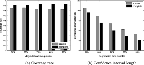
We also evaluate the accuracy of the confidence interval estimates introduced in Section 4. In Figure 7 we present the coverage rate level and the mean of the confidence interval length at the degradation lifetime percentiles 50%, 60%, 70%, 80% and 90%. The confidence interval level is . The coverage rate is higher for complete signals than for sparse signals throughout all percentiles, but the difference is insignificant. The coverage rate for both complete and sparse signals is approximately equal to the confidence level . Moreover, the mean length decreases for higher percentiles, implying that the accuracy of the residual life estimate increases as the latest observation time point is closer to the failure time.
7.1.2 Results and analysis of Model 2
In the following analysis we still use Model 1 as the assumed parametric model and its derived residual life distribution as the benchmark. This assumed parametric model correctly captures the mean degradation trend of Model 2 but not the underlying covariance structure of the degradation process. It is worth mentioning that most existing parametric approaches focus on identification of the functional form for the underlying degradation trend, ignoring the underlying covariance structure.
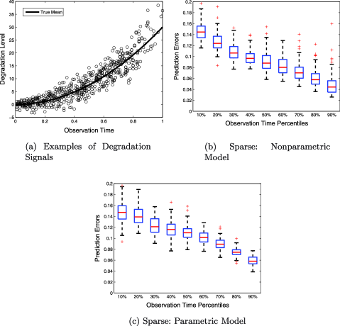
The results in Figure 8 indicate that our nonparametric model is more accurate than the assumed parametric model in predicting the residual life. This is because our proposed nonparametric approach, which is FPCA-based, cannot only estimate the mean trend accurately but also capture the dominant modes of the covariance structure correctly. In contrast, parametric models are not flexible enough to accurately capture the underlying covariance structure.
We also compute the prediction error results for cases when the observed degradation signals are complete, fragmented or sparse, and also when the scores and errors follow different distributions. Detailed results can be found in the supplementary materials [Zhou, Serban and Gebraeel (2010)].
7.1.3 Results and analysis of Model 3
We discuss this in the supplementary materials [Zhou, Serban and Gebraeel (2010)].
8 Discussions
In this paper we propose an Empirical Bayesian method for predicting the degradation of a partially degraded component or system. Specifically, we assume that the degradation process has unknown mean and covariance, which can be estimated through a nonparametric approach using a historical database of degradation signals used to estimate the prior distribution of the degradation process. These training degradation signals may be completely or incompletely observed, that is, may be in the form of sparsely observed signals or fragmented signals.
Our degradation modeling and monitoring approach relies on a series of assumptions:
-
•
The degradation signals follow a Gaussian process.
-
•
The time points at which the training signals have been observed cover the time domain cumulatively.
-
•
The degradation signal of the new component does not cross back the threshold .
From our simulation results, departures from the Gaussian assumption will insignificantly alter the residual life estimates when a large number of training signals are observed, as discussed in Section 7. This property is inherited from the robustness of the FPCA approach used in estimating the empirical prior distribution.
Under sparse sampling, the selection of the observation times of the training degradation signals impacts the accuracy of the degradation prior modeling. For example, if the degradation signals are uniformly but sparsely sampled, the degradation process will not be adequately observed at the later extreme time point , since few components will survive up to this time point. Consequently, uniform sampling compromises the accuracy of the mean and covariance estimates of the prior degradation process, which, in turn, compromises the accuracy of the residual life estimate. In the simulation study we show that the accuracy of the residual life estimates is low for the traditional uniform sampling as compared to the accuracy of the estimates under nonuniform sampling. Thus, the second assumption is ensured under nonuniform sampling but not uniform sparse sampling (see Section 5).
The third assumption in our modeling approach relies on that the experimenter will shut off or replace the component shortly after it degraded beyond the failure threshold .
In this paper we have applied the nonparametric approach to crack growth data with a wide applicability, for example, in infrastructure (bridges, steel structures), maritime (hulls of oil tankers), aeronautical (aircraft fuselage), energy (vanes of gas turbines) and others. This case study demonstrates the accuracy of the nonparametric approach introduced in this paper as compared to random effects parametric models which impose constrains on the shape of the trend and the covariance . Other potential applications are relevant to LED data that could be found in Yu and Tseng (1998), Liao and Tseng (2006) and Tseng and Peng (2007).
Acknowledgments
We would like to thank the Editor, anonymous Associate Editor and anonymous reviewers for their constructive and thoughtful comments on this manuscript.
Additional results \slink[doi]10.1214/10-AOAS448SUPP \slink[url]http://lib.stat.cmu.edu/aoas/448/supplement.pdf \sdatatype.pdf \sdescriptionIn this supplemental file we provide some additional results of the crack growth data study and the simulation study.
References
- Bogdanoff and Kozin (1985) {bbook}[auto:STB—2011-01-28—17:37:40] \bauthor\bsnmBogdanoff, \bfnmJ. L.\binitsJ. L. and \bauthor\bsnmKozin, \bfnmF.\binitsF. (\byear1985). \btitleProbabilistic Models of Cummulative Damage. \bpublisherWiley, \baddressNew York. \endbibitem
- Cross, Makeev and Armanios (2006) {barticle}[auto:STB—2011-01-28—17:37:40] \bauthor\bsnmCross, \bfnmR. J.\binitsR. J., \bauthor\bsnmMakeev, \bfnmA.\binitsA. and \bauthor\bsnmArmanios, \bfnmE.\binitsE. (\byear2006). \btitleA comparison of predictions from probabilistic crack growth models inferred from Virkler’s data. \bjournalJ. ASTM International \bvolume3. DOI: 101520/JAI100574. \endbibitem
- Davison and Hinkley (1997) {bbook}[mr] \bauthor\bsnmDavison, \bfnmA. C.\binitsA. C. and \bauthor\bsnmHinkley, \bfnmD. V.\binitsD. V. (\byear1997). \btitleBootstrap Methods and Their Application. \bseriesCambridge Series in Statistical and Probabilistic Mathematics \bvolume1. \bpublisherCambridge Univ. Press, \baddressCambridge. \bidmr=1478673 \endbibitem
- Doksum and Hoyland (1992) {barticle}[auto:STB—2011-01-28—17:37:40] \bauthor\bsnmDoksum, \bfnmK. A.\binitsK. A. and \bauthor\bsnmHoyland, \bfnmA.\binitsA. (\byear1992). \btitleModels for variable-stress accelerated life testing experiments based on Wiener processes and the inverse Gaussian distribution. \bjournalTechnometrics \bvolume34 \bpages74–82. \endbibitem
- Efron and Tibshirani (1993) {bbook}[mr] \bauthor\bsnmEfron, \bfnmBradley\binitsB. and \bauthor\bsnmTibshirani, \bfnmRobert J.\binitsR. J. (\byear1993). \btitleAn Introduction to the Bootstrap. \bseriesMonographs on Statistics and Applied Probability \bvolume57. \bpublisherChapman and Hall, \baddressNew York. \bidmr=1270903 \endbibitem
- Fan and Yao (2003) {bbook}[mr] \bauthor\bsnmFan, \bfnmJianqing\binitsJ. and \bauthor\bsnmYao, \bfnmQiwei\binitsQ. (\byear2003). \btitleNonlinear Time Series: Nonparametric and Parametric Methods. \bpublisherSpringer, \baddressNew York. \biddoi=10.1007/b97702, mr=1964455 \endbibitem
- Gebraeel (2006) {barticle}[auto:STB—2011-01-28—17:37:40] \bauthor\bsnmGebraeel, \bfnmN.\binitsN. (\byear2006). \btitleSensory updated residual life distribution for components with exponential degradation patterns. \bjournalIEEE Transactions on Automation Science and Engineering \bvolume3 \bpages382–393. \endbibitem
- Gebraeel et al. (2005) {barticle}[auto:STB—2011-01-28—17:37:40] \bauthor\bsnmGebraeel, \bfnmN.\binitsN., \bauthor\bsnmLawley, \bfnmM.\binitsM., \bauthor\bsnmLi, \bfnmR.\binitsR. and \bauthor\bsnmRyan, \bfnmJ.\binitsJ. (\byear2005). \btitleResidual-life distributions from component degradation signals: A Bayesian approach. \bjournalIIE Transactions \bvolume37 \bpages543–557. \endbibitem
- James, Hastie and Sugar (2000) {barticle}[mr] \bauthor\bsnmJames, \bfnmGareth M.\binitsG. M., \bauthor\bsnmHastie, \bfnmTrevor J.\binitsT. J. and \bauthor\bsnmSugar, \bfnmCatherine A.\binitsC. A. (\byear2000). \btitlePrincipal component models for sparse functional data. \bjournalBiometrika \bvolume87 \bpages587–602. \biddoi=10.1093/biomet/87.3.587, mr=1789811 \endbibitem
- Karhunen (1947) {bmisc}[auto:STB—2011-01-28—17:37:40] \bauthor\bsnmKarhunen, \bfnmK.\binitsK. (\byear1947). \bhowpublishedÜber lineare Methoden in der Wahrscheinlichkeitsrechnung. Suomalainen Tiedeakatemia, Finland. \endbibitem
- Kotulski (1998) {barticle}[auto:STB—2011-01-28—17:37:40] \bauthor\bsnmKotulski, \bfnmZ. A.\binitsZ. A. (\byear1998). \btitleOn efficiency of identification of a stochastic crack propagation model based on Virkler experimental data. \bjournalArchives of Mechanics \bvolume5 \bpages829–847. \endbibitem
- Liao and Tseng (2006) {barticle}[auto:STB—2011-01-28—17:37:40] \bauthor\bsnmLiao, \bfnmC. M.\binitsC. M. and \bauthor\bsnmTseng, \bfnmS. T.\binitsS. T. (\byear2006). \btitleOptimal design for step-stress accelerated degradation tests. \bjournalIEEE Transactions on Reliability \bvolume55. \endbibitem
- Loève (1945) {barticle}[auto:STB—2011-01-28—17:37:40] \bauthor\bsnmLoève, \bfnmM.\binitsM. (\byear1945). \btitleFunctions aleatoire de second order. \bjournalComptes Rendus Acad. Sci. \bvolume220. \endbibitem
- Lu and Meeker (1993) {barticle}[mr] \bauthor\bsnmLu, \bfnmC. Joseph\binitsC. J. and \bauthor\bsnmMeeker, \bfnmWilliam Q.\binitsW. Q. (\byear1993). \btitleUsing degradation measures to estimate a time-to-failure distribution. \bjournalTechnometrics \bvolume35 \bpages161–174. \bidmr=1225093 \endbibitem
- Müller and Zhang (2005) {barticle}[mr] \bauthor\bsnmMüller, \bfnmHans-Georg\binitsH.-G. and \bauthor\bsnmZhang, \bfnmYing\binitsY. (\byear2005). \btitleTime-varying functional regression for predicting remaining lifetime distributions from longitudinal trajectories. \bjournalBiometrics \bvolume61 \bpages1064–1075. \biddoi=10.1111/j.1541-0420.2005.00378.x, mr=2216200 \endbibitem
- Nelson (1990) {bbook}[auto:STB—2011-01-28—17:37:40] \bauthor\bsnmNelson, \bfnmW.\binitsW. (\byear1990). \btitleAccelerated Testing Statistical Models, Test Plans and Data Analysis. \bpublisherWiley, \baddressNew York. \endbibitem
- Padgett and Tomlinson (2004) {barticle}[mr] \bauthor\bsnmPadgett, \bfnmW. J.\binitsW. J. and \bauthor\bsnmTomlinson, \bfnmMeredith A.\binitsM. A. (\byear2004). \btitleInference from accelerated degradation and failure data based on Gaussian process models. \bjournalLifetime Data Anal. \bvolume10 \bpages191–206. \biddoi=10.1023/B:LIDA.0000030203.49001.b6, mr=2081721 \endbibitem
- Park and Padgett (2006) {barticle}[auto:STB—2011-01-28—17:37:40] \bauthor\bsnmPark, \bfnmC.\binitsC. and \bauthor\bsnmPadgett, \bfnmW. J.\binitsW. J. (\byear2006). \btitleStochastic degradation models with several accelerating variables. \bjournalIEEE Transactions on Reliability \bvolume55 \bpages379–390. \endbibitem
- Pettit and Young (1999) {barticle}[mr] \bauthor\bsnmPettit, \bfnmL. I.\binitsL. I. and \bauthor\bsnmYoung, \bfnmK. D. S.\binitsK. D. S. (\byear1999). \btitleBayesian analysis for inverse Gaussian lifetime data with measures of degradation. \bjournalJ. Statist. Comput. Simulation \bvolume63 \bpages217–234. \biddoi=10.1080/00949659908811954, mr=1703821 \endbibitem
- Ramsay and Silverman (1997) {bbook}[mr] \bauthor\bsnmRamsay, \bfnmJ. O.\binitsJ. O. and \bauthor\bsnmSilverman, \bfnmB. W.\binitsB. W. (\byear1997). \btitleFunctional Data Analysis. \bpublisherSpringer, \baddressNew York. \endbibitem
- Rice and Silverman (1991) {barticle}[mr] \bauthor\bsnmRice, \bfnmJohn A.\binitsJ. A. and \bauthor\bsnmSilverman, \bfnmB. W.\binitsB. W. (\byear1991). \btitleEstimating the mean and covariance structure nonparametrically when the data are curves. \bjournalJ. Roy. Statist. Soc. Ser. B \bvolume53 \bpages233–243. \bidmr=1094283 \endbibitem
- Tseng and Peng (2007) {barticle}[auto:STB—2011-01-28—17:37:40] \bauthor\bsnmTseng, \bfnmS. T.\binitsS. T. and \bauthor\bsnmPeng, \bfnmC. Y.\binitsC. Y. (\byear2007). \btitleStochastic diffusion modeling of degradation data. \bjournalJ. Data Sci. \bvolume5 \bpages315–333. \endbibitem
- Virkler, Hillberry and Goel (1979) {barticle}[auto:STB—2011-01-28—17:37:40] \bauthor\bsnmVirkler, \bfnmD. A.\binitsD. A., \bauthor\bsnmHillberry, \bfnmB. M.\binitsB. M. and \bauthor\bsnmGoel, \bfnmP. K.\binitsP. K. (\byear1979). \btitleThe statistical nature of fatigue crack propagation. \bjournalJ. Eng. Mater. Technol. \bvolume101 \bpages148–153. \endbibitem
- Yao, Müller and Wang (2005) {barticle}[mr] \bauthor\bsnmYao, \bfnmFang\binitsF., \bauthor\bsnmMüller, \bfnmHans-Georg\binitsH.-G. and \bauthor\bsnmWang, \bfnmJane-Ling\binitsJ.-L. (\byear2005). \btitleFunctional data analysis for sparse longitudinal data. \bjournalJ. Amer. Statist. Assoc. \bvolume100 \bpages577–590. \biddoi=10.1198/016214504000001745, mr=2160561 \endbibitem
- Yu and Tseng (1998) {barticle}[auto:STB—2011-01-28—17:37:40] \bauthor\bsnmYu, \bfnmH. F.\binitsH. F. and \bauthor\bsnmTseng, \bfnmS. T.\binitsS. T. (\byear1998). \btitleOn-line procedure for terminating an accelerated degradation test. \bjournalStatist. Sinica \bvolume8 \bpages207–220. \endbibitem
- Zhou, Serban and Gebraeel (2010) {bmisc}[auto:STB—2011-01-28—17:37:40] \bauthor\bsnmZhou, \bfnmR. R.\binitsR. R., \bauthor\bsnmSerban, \bfnmN.\binitsN. and \bauthor\bsnmGebraeel, \bfnmN.\binitsN. (\byear2010). \bhowpublishedSupplement to “Degradation modeling applied to residual lifetime prediction using functional data analysis.” Ann. Appl. Statist. DOI: 10.1214/10-AOAS448SUPP. \endbibitem