Search for sterile neutrinos at reactors

Osamu Yasuda E-mail: yasuda˙at˙phys.se.tmu.ac.jp Department of Physics, Tokyo Metropolitan University, Hachioji, Tokyo 192-0397, Japan
Abstract

The sensitivity to the sterile neutrino mixing at very short baseline reactor neutrino experiments is investigated. In the case of conventional (thermal neutron) reactors it is found that the sensitivity is lost for Δm2greater-than-or-equivalent-toΔsuperscript𝑚2absent\Delta m^{2}\gtrsim 1 eV2 due to smearing of the reactor core size. On the other hand, in the case of an experimental fast neutron reactor Joyo, because of its small size, sensitivity to sin22θ14superscript22subscript𝜃14\sin^{2}2\theta_{14} can be as good as 0.03 for Δm2similar-toΔsuperscript𝑚2absent\Delta m^{2}\sim several eV2 with the Bugey-like detector setup.

pacs:
14.60.Pq,25.30.Pt,28.41.-i

I Introduction

Since the LSND group announced the anomaly which suggests neutrino oscillations with mass squared difference of 𝒪𝒪{\cal O}(1) eV2Athanassopoulos:1996jb ; Athanassopoulos:1997pv ; Aguilar:2001ty , schemes with sterile neutrinos have attracted a lot of attention. This is because the standard three flavor scheme has only two independent mass squared differences, i.e., Δm212=Δm28×105Δsubscriptsuperscript𝑚221Δsubscriptsuperscript𝑚2direct-productsimilar-to-or-equals8superscript105\Delta m^{2}_{21}=\Delta m^{2}_{\odot}\simeq 8\times 10^{-5}eV2 for the solar neutrino oscillation, and |Δm312|=Δmatm22.4×103Δsubscriptsuperscript𝑚231Δsubscriptsuperscript𝑚2atmsimilar-to-or-equals2.4superscript103|\Delta m^{2}_{31}|=\Delta m^{2}_{\text{atm}}\simeq 2.4\times 10^{-3}eV2 for the atmospheric neutrino oscillation, and it does not have room for the mass squared difference of 𝒪𝒪{\cal O}(1) eV2. The extra state has to be sterile neutrino, which is singlet with respect to the gauge group of the Standard Model, because the number of weakly interacting light neutrinos has to be three from the LEP data.Nakamura:2010zzi

The LSND anomaly has been tested by the MiniBooNE experiment. While the MiniBooNE data on the neutrino mode AguilarArevalo:2007it disfavors the region suggested by LSND, their data on the anti-neutrino mode AguilarArevalo:2010wv seems to be consistent with the LSND data.

Recently the flux of the reactor neutrino was recalculated in Ref. Mueller:2011nm and it was reported that the normalization is shifted by about +3% on average.111 The increase in the flux claimed by Ref. Mueller:2011nm was confirmed by an independent calculation in Ref. Huber:2011wv . Then a re-analysis of 19 reactor neutrino results at short baselines Mention:2011rk in the light of new reactor neutrino spectra Mueller:2011nm may indicate neutrino oscillation at Δm2greater-than-or-equivalent-toΔsuperscript𝑚2absent\Delta m^{2}\gtrsim1eV2.

Reactor experiments with more than one detector have attracted much attention as a possibility to measure θ13subscript𝜃13\theta_{13} precisely Kozlov:2001jv ; Minakata:2002jv ; Huber:2003pm ; Anderson:2004pk , and three experiments Ardellier:2004ui ; Ahn:2010vy ; Guo:2007ug are now either running or expected to start soon. In the three flavor case with |Δm312|=2.4×10³Δsubscriptsuperscript𝑚2312.4superscript103|\Delta m^{2}_{31}|=2.4\times 10^{-3}eV2, it was shown assuming infinite statistics that the optimized baseline lengths LFsubscript𝐿𝐹L_{F} and LNsubscript𝐿𝑁L_{N} for the far and near detectors are LFsimilar-to-or-equalssubscript𝐿𝐹absentL_{F}\simeq1.8km and LNsimilar-to-or-equalssubscript𝐿𝑁absentL_{N}\simeq0km in the rate analysis Yasuda:2004dd ; Sugiyama:2004bv , while they are LFsimilar-to-or-equalssubscript𝐿𝐹absentL_{F}\simeq10.6km and LNsimilar-to-or-equalssubscript𝐿𝑁absentL_{N}\simeq8.4km in the spectrum analysis Sugiyama:2005ir . Unfortunately, in order to justify the assumption on negligible statistical errors for Lsimilar-to𝐿absentL\sim10km, one would need unrealistically huge detectors, so one is forced to choose the baseline lengths which are optimized for the rate analysis for Δm2=2.4×10³Δsuperscript𝑚22.4superscript103\Delta m^{2}=2.4\times 10^{-3}eV2. On the other hand, if we perform an oscillation experiment to probe Δm2𝒪similar-toΔsuperscript𝑚2𝒪\Delta m^{2}\sim{\cal O}(1) eV2, it becomes realistic to place the detectors at the baseline lengths which are optimized for the spectrum analysis (See Sect. 4 in the published version of Ref. Sugiyama:2005ir ).

In this paper we discuss the sensitivity of very short line reactor experiments to the sterile neutrino mixing for Δm2𝒪similar-toΔsuperscript𝑚2𝒪\Delta m^{2}\sim{\cal O}(1) eV2 in the so-called (3+1)-scheme.222According to Ref. Kopp:2011qd , the so-called (3+2)-scheme Sorel:2003hf gives a better fit to the global data than the (3+1)-scheme does. However, we are mainly interested here in the potential sensitivity to the sterile neutrino mixing for Δm2𝒪similar-toΔsuperscript𝑚2𝒪\Delta m^{2}\sim{\cal O}(1) eV2, and for simplicity we will discuss the (3+1)-scheme, leaving the analysis of the (3+2)-scheme for the future. Proposals have been made to test the bound of the Bugey reactor experiment Declais:1994su on the sterile neutrino mixing angle using a reactor nucifer ,333 See, e.g., Refs. Sugiyama:2005ir (the published version), Latimer:2007qe ; deGouvea:2008qk for earlier works on search for sterile neutrinos at a reactor. an accelerator Agarwalla:2009em ; Rubbia:2011 , and a β𝛽\beta-source Cribier:2011fv .

Throughout this paper we discuss the case with a single reactor and two detectors, which have an advantage to cancel the systematic errors that are correlated between detectors. The conditions of the detectors are assumed to be the same as those of the Bugey experiment.

In Sect. 2 we briefly review the four neutrino schemes. In Sect. 3 we evaluate the sensitivity of very short line reactor experiments to the sterile neutrino mixing. In Sect. 4 we summarize our results. In Appendix A we give some details to get an analytical expression for χ2superscript𝜒2\chi^{2}.

II Four neutrino schemes

Four-neutrino schemes consist of one extra sterile state in addition to the three weakly interacting ones. Depending on whether one or two mass eigenstate(s) are separated from the others by the largest mass-squared gap, the schemes are called (3+1)- and (2+2)-schemes. The (2+2) schemes are excluded by the solar and atmospheric neutrino data Maltoni:2004ei , so we will not discuss the (2+2) schemes in this paper. In the (3+1) schemes, on the other hand, the phenomenology of solar and atmospheric oscillations is approximately the same as that of the three flavor framework, so as far as the tension between the solar and atmospheric constraints are concerned, the (3+1) schemes do not have any problem. However, if we try to account for LSND and all other negative results of the short baseline experiments, then the (3+1) schemes have a problem. To explain the LSND data while satisfying the constraints from other disappearance experiments, the oscillation probabilities of the appearance and disappearance channels have to satisfy the following relation Okada:1996kw ; Bilenky:1996rw :

sin22θLSND(Δm2)<14sin22θBugey(Δm2)sin22θCDHSW(Δm2)superscript22subscript𝜃LSNDΔsuperscript𝑚214superscript22subscript𝜃BugeyΔsuperscript𝑚2superscript22subscript𝜃CDHSWΔsuperscript𝑚2\displaystyle\sin^{2}2\theta_{\mbox{\rm\tiny LSND}}(\Delta m^{2})<\frac{1}{4}\,\sin^{2}2\theta_{\mbox{\rm\scriptsize Bugey}}(\Delta m^{2})\cdot\sin^{2}2\theta_{\mbox{\rm\tiny CDHSW}}(\Delta m^{2}) (1)

where θLSND(Δm2)subscript𝜃LSNDΔsuperscript𝑚2\theta_{\mbox{\rm\tiny LSND}}(\Delta m^{2}), θCDHSW(Δm2)subscript𝜃CDHSWΔsuperscript𝑚2\theta_{\mbox{\rm\tiny CDHSW}}(\Delta m^{2}), θBugey(Δm2)subscript𝜃BugeyΔsuperscript𝑚2\theta_{\mbox{\rm\scriptsize Bugey}}(\Delta m^{2}) are the value of the effective two-flavor mixing angle as a function of the mass squared difference Δm2Δsuperscript𝑚2\Delta m^{2} in the allowed region for LSND (ν¯μν¯esubscript¯𝜈𝜇subscript¯𝜈𝑒\bar{\nu}_{\mu}\rightarrow\bar{\nu}_{e}), the CDHSW experiment Dydak:1983zq (νμνμsubscript𝜈𝜇subscript𝜈𝜇\nu_{\mu}\rightarrow\nu_{\mu}), and the Bugey experiment Declais:1994su (ν¯eν¯esubscript¯𝜈𝑒subscript¯𝜈𝑒\bar{\nu}_{e}\rightarrow\bar{\nu}_{e}), respectively. The reason that the (3+1)-scheme to explain LSND has been disfavored until Refs. Mueller:2011nm ; Mention:2011rk appeared is because Eq. (1) is not satisfied for any value of Δm2Δsuperscript𝑚2\Delta m^{2}, if we adopt the allowed regions in Refs. Dydak:1983zq and Declais:1994su . However, if the flux of the reactor neutrino is slightly larger than the one used in the Bugey analysis Declais:1994su , the allowed region becomes slightly wider and we have more chance to satisfy Eq. (1).

In this paper we will use the following parametrization for the mixing matrix, adopted in Ref. Maltoni:2007zf :

U=R34(θ34, 0)R24(θ24, 0)R23(θ23,δ3)R14(θ14, 0)R13(θ13,δ2)R12(θ12,δ1),𝑈subscript𝑅34subscript𝜃34 0subscript𝑅24subscript𝜃24 0subscript𝑅23subscript𝜃23subscript𝛿3subscript𝑅14subscript𝜃14 0subscript𝑅13subscript𝜃13subscript𝛿2subscript𝑅12subscript𝜃12subscript𝛿1\displaystyle U=R_{34}(\theta_{34},\,0)\;R_{24}(\theta_{24},\,0)\;R_{23}(\theta_{23},\,\delta_{3})\;R_{14}(\theta_{14},\,0)\;R_{13}(\theta_{13},\,\delta_{2})\;R_{12}(\theta_{12},\,\delta_{1})\,,

where Rjk(θjk,δl)subscript𝑅𝑗𝑘subscript𝜃𝑗𝑘subscript𝛿𝑙R_{jk}(\theta_{jk},\ \delta_{l}) are the complex rotation matrices in the jk𝑗𝑘jk-plane defined as:

[Rjk(θjk,δl)]pq=δpq+(cosθjk1)(δjpδjq+δkpδkq)+sinθjk(eiδlδjpδkqeiδlδjqδkp).subscriptdelimited-[]subscript𝑅𝑗𝑘subscript𝜃𝑗𝑘subscript𝛿𝑙𝑝𝑞subscript𝛿𝑝𝑞subscript𝜃𝑗𝑘1subscript𝛿𝑗𝑝subscript𝛿𝑗𝑞subscript𝛿𝑘𝑝subscript𝛿𝑘𝑞subscript𝜃𝑗𝑘superscript𝑒𝑖subscript𝛿𝑙subscript𝛿𝑗𝑝subscript𝛿𝑘𝑞superscript𝑒𝑖subscript𝛿𝑙subscript𝛿𝑗𝑞subscript𝛿𝑘𝑝\displaystyle[R_{jk}(\theta_{jk},\ \delta_{l})]_{pq}=\delta_{pq}+(\cos\theta_{jk}-1)(\delta_{jp}\delta_{jq}+\delta_{kp}\delta_{kq})+\sin\theta_{jk}(e^{-i\delta_{l}}\delta_{jp}\delta_{kq}-e^{i\delta_{l}}\delta_{jq}\delta_{kp}).

With this parametrization, for the very short baseline reactor experiments, where the average neutrino energy E𝐸E is approximately 4MeV and the baseline length is about 10m, we have |Δmjk2L/4E|1(j,k=1,2,3)|\Delta m^{2}_{jk}L/4E|\ll 1~{}(j,k=1,2,3), so that the disappearance probability is given by

P(ν¯eν¯e)=1sin22θ14sin2(Δm412L4E)𝑃subscript¯𝜈𝑒subscript¯𝜈𝑒1superscript22subscript𝜃14superscript2Δsubscriptsuperscript𝑚241𝐿4𝐸\displaystyle P(\bar{\nu}_{e}\to\bar{\nu}_{e})=1-\sin^{2}2\theta_{14}\,\sin^{2}\left(\frac{\Delta m^{2}_{41}L}{4E}\right) (2)

to a good approximation. Eq. (2) is the formula which will be used in the oscillation analysis throughout this paper.

III Sensitivity to sin22θ14superscript22subscript𝜃14\sin^{2}{2\theta_{14}} by a spectral analysis

Throughout this paper we discuss the case with a single reactor and two detectors. The detectors are assumed to be of the Bugey type, i.e., liquid scintillation detector of volume 600 liters with the detection efficiency which yields about 90,000 events at L𝐿L=15m from a reactor of a power 2.8GW after running for 1800 hours. Also for simplicity, we assume in this paper that the near and far detectors are identical and have the same sizes of systematic errors.

To evaluate the sensitivity to sin22θ14superscript22subscript𝜃14\sin^{2}{2\theta_{14}}, we introduce the following χ2superscript𝜒2\chi^{2} which was adopted in Ref. Sugiyama:2005ir :

χ2superscript𝜒2\displaystyle\displaystyle\chi^{2} =\displaystyle= minαs{A=N,Fi=1n1(tiAσiA)2[miAtiA(1+α+αA+αi)αcalAtiAviA]2\displaystyle\min_{\alpha^{\prime}s}\Bigg{\{}\displaystyle\sum_{A=N,F}\sum_{i=1}^{n}\frac{1}{(t^{A}_{i}\sigma^{A}_{i})^{2}}\left[m^{A}_{i}-t^{A}_{i}(1+\alpha+\alpha^{A}+\alpha_{i})-\alpha_{\text{cal}}^{A}t^{A}_{i}v^{A}_{i}\right]^{2} (3)
+\displaystyle+ A=N,F[(αAσdB)2+(αcalAσcal)2]+i=1n(αiσDb)2+(ασDB)2}.\displaystyle\displaystyle\sum_{A=N,F}\left[\left(\frac{\alpha^{A}}{\sigma_{\text{dB}}}\right)^{2}+\left(\frac{\alpha_{\text{cal}}^{A}}{\sigma_{\text{cal}}}\right)^{2}\right]+\displaystyle\sum_{i=1}^{n}\left(\frac{\alpha_{i}}{\sigma_{\text{Db}}}\right)^{2}+\left(\frac{\alpha}{\sigma_{\text{DB}}}\right)^{2}\Bigg{\}}.

Here, miAsubscriptsuperscript𝑚𝐴𝑖m^{A}_{i} is the number of events to be measured at the near (A=N𝐴𝑁A=N) and far (A=F𝐴𝐹A=F) for the i𝑖i-th energy bin with the neutrino oscillation444 As we will see below, in the spectrum analysis, unlike in the rate one, it is not necessary for the near detector to have events without oscillation, since the dominant term in χ2superscript𝜒2\chi^{2} looks at the difference between the maximum and minimum of the oscillation pattern. In fact, in Fig. 1 below there are regions in which LNLFsubscript𝐿𝑁subscript𝐿𝐹L_{N}\geq L_{F}. Therefore, it may be misleading to call the detector at the shorter baseline length the near detector. Nevertheless, we use these words throughout this paper for simplicity., and tiAsubscriptsuperscript𝑡𝐴𝑖t^{A}_{i} is the theoretical prediction without the oscillation. (σiA)2superscriptsubscriptsuperscript𝜎𝐴𝑖2(\sigma^{A}_{i})^{2} is the uncorrelated error which consists of the statistical plus uncorrelated bin-to-bin systematic error:

(tiAσiA)2=tiA+(tiAσdbA)2,superscriptsubscriptsuperscript𝑡𝐴𝑖subscriptsuperscript𝜎𝐴𝑖2subscriptsuperscript𝑡𝐴𝑖superscriptsubscriptsuperscript𝑡𝐴𝑖subscriptsuperscript𝜎𝐴db2\displaystyle(t^{A}_{i}\sigma^{A}_{i})^{2}=t^{A}_{i}+\left(t^{A}_{i}\sigma^{A}_{\text{db}}\right)^{2},

where σdbAsubscriptsuperscript𝜎𝐴db\sigma^{A}_{\text{db}} is the uncorrelated bin-to-bin systematic error. For simplicity we assume that sizes of the bin-to-bin uncorrelated systematic errors of the detectors and of the flux are independent of the energy. Also we take the choice of the bins in such a way that the number of events for each bin is equal: tiA=tA(i=1,,n)subscriptsuperscript𝑡𝐴𝑖superscript𝑡𝐴𝑖1𝑛t^{A}_{i}=t^{A}~{}(i=1,\cdots,n). α𝛼\alpha is a variable which corresponds to a common overall normalization error σDBsubscript𝜎DB\sigma_{\text{DB}} for the number of events. αA(A=N,F)superscript𝛼𝐴𝐴𝑁𝐹\alpha^{A}~{}(A=N,F) is a variable which introduces the detector-specific uncertainties σdBsubscript𝜎dB\sigma_{\text{dB}} of the near and far detectors. αi(i=1,,n)subscript𝛼𝑖𝑖1𝑛\alpha_{i}~{}(i=1,\cdots,n) is a variable for an uncertainty σDbsubscript𝜎Db\sigma_{\text{Db}} of the theoretical prediction for each energy bin which is uncorrelated between different energy bins.555 Here we follow the notation for the systematic errors in Ref. Sugiyama:2005ir . The first suffix of σ𝜎\sigma stands for the property for the systematic error with respect to the detectors while the second is with respect to bins, and capital (small) letter stands for a correlated (uncorrelated) systematic error. The correspondence for the notation in Ref. Huber:2003pm is as follows: σdb=σexpsubscript𝜎dbsubscript𝜎exp\sigma_{\text{db}}=\sigma_{\text{exp}}, σdB=σbsubscript𝜎dBsubscript𝜎𝑏\sigma_{\text{dB}}=\sigma_{b}, σDb=σshapesubscript𝜎Dbsubscript𝜎shape\sigma_{\text{Db}}=\sigma_{\text{shape}}, σDB=σasubscript𝜎DBsubscript𝜎𝑎\sigma_{\text{DB}}=\sigma_{a}. αcalA(A=N,F)superscriptsubscript𝛼cal𝐴𝐴𝑁𝐹\alpha_{\text{cal}}^{A}~{}(A=N,F) is a variable which introduces an energy calibration uncertainty σcalsubscript𝜎cal\sigma_{\text{cal}} and comes in the theoretical prediction in the form of (1+αcalA)E1superscriptsubscript𝛼cal𝐴𝐸(1+\alpha_{\text{cal}}^{A})E instead of the observed energy E𝐸E. Thus, the deviation viAsubscriptsuperscript𝑣𝐴𝑖v^{A}_{i} (divided by the expected number of events) from the theoretical prediction tiAsubscriptsuperscript𝑡𝐴𝑖t^{A}_{i} due to this uncertainty can be written as

viA=limαcalA01αcalAtiA[NpT4πLA2𝑑E(1+αcalA)Ei(1+αcalA)Ei+1𝑑ER(Ee,E)ϵ(E)F(E)σ(E)tiA],subscriptsuperscript𝑣𝐴𝑖subscriptsuperscriptsubscript𝛼cal𝐴01superscriptsubscript𝛼cal𝐴subscriptsuperscript𝑡𝐴𝑖delimited-[]subscript𝑁𝑝𝑇4𝜋superscriptsubscript𝐿𝐴2differential-d𝐸superscriptsubscript1superscriptsubscript𝛼cal𝐴subscript𝐸𝑖1superscriptsubscript𝛼cal𝐴subscript𝐸𝑖1differential-dsuperscript𝐸𝑅subscript𝐸𝑒superscript𝐸italic-ϵ𝐸𝐹𝐸𝜎𝐸subscriptsuperscript𝑡𝐴𝑖\displaystyle v^{A}_{i}=\lim_{\alpha_{\text{cal}}^{A}\rightarrow 0}\frac{1}{\alpha_{\text{cal}}^{A}t^{A}_{i}}\left[\frac{N_{p}T}{4\pi L_{A}^{2}}\int dE\int_{(1+\alpha_{\text{cal}}^{A})E_{i}}^{(1+\alpha_{\text{cal}}^{A})E_{i+1}}dE^{\prime}\,R(E_{e},E^{\prime})\epsilon(E)F(E)\sigma(E)-t^{A}_{i}\right], (4)

with

tiANpT4πLA2𝑑EEiEi+1𝑑ER(Ee,E)ϵ(E)F(E)σ(E).subscriptsuperscript𝑡𝐴𝑖subscript𝑁𝑝𝑇4𝜋superscriptsubscript𝐿𝐴2differential-d𝐸superscriptsubscriptsubscript𝐸𝑖subscript𝐸𝑖1differential-dsuperscript𝐸𝑅subscript𝐸𝑒superscript𝐸italic-ϵ𝐸𝐹𝐸𝜎𝐸\displaystyle t^{A}_{i}\equiv\frac{N_{p}T}{4\pi L_{A}^{2}}\int dE\int_{E_{i}}^{E_{i+1}}dE^{\prime}\,R(E_{e},E^{\prime})\epsilon(E)F(E)\sigma(E). (5)

In Eqs. (4) and (5), Npsubscript𝑁𝑝N_{p} is the number of target protons in the detector, T𝑇T denotes the exposure time, LAsubscript𝐿𝐴L_{A} is the baseline for the detector A𝐴A, F(E)𝐹𝐸F(E) is the flux of ν¯esubscript¯𝜈𝑒\bar{\nu}_{e}, and σ(E)𝜎𝐸\sigma(E) is the cross section of the inverse β𝛽\beta decay ν¯e+pn+e+subscript¯𝜈𝑒𝑝𝑛superscript𝑒\bar{\nu}_{e}+p\to n+e^{+}. E𝐸E is the energy of the incident ν¯esubscript¯𝜈𝑒\bar{\nu}_{e} and it is related to the positron energy Eesubscript𝐸𝑒E_{e} and the masses mnsubscript𝑚𝑛m_{n}, mpsubscript𝑚𝑝m_{p} of a neutron and a proton by E=Ee+mnmp=Ee+1.3𝐸subscript𝐸𝑒subscript𝑚𝑛subscript𝑚𝑝subscript𝐸𝑒1.3E=E_{e}+m_{n}-m_{p}=E_{e}+1.3 MeV. Esuperscript𝐸E^{\prime} is the measured positron energy and we will assume that the energy resolution is given by 8%/Epercent8𝐸8\%/\sqrt{E}, i.e., R(Ee,E)=R(Emn+mp,E)𝑅subscript𝐸𝑒superscript𝐸𝑅𝐸subscript𝑚𝑛subscript𝑚𝑝superscript𝐸R(E_{e},E^{\prime})=R(E-m_{n}+m_{p},E^{\prime}) is a Gaussian function which describes the energy resolution and is given by R(Ee,E)=(1/2πσ)exp[(EeE)2/2σ2]𝑅subscript𝐸𝑒superscript𝐸12𝜋𝜎superscriptsubscript𝐸𝑒superscript𝐸22superscript𝜎2R(E_{e},E^{\prime})=(1/\sqrt{2\pi}\sigma)\exp[-(E_{e}-E^{\prime})^{2}/2\sigma^{2}], where σ=0.08(Ee+me)/MeV=0.08(E0.8/MeV)/MeV𝜎0.08subscript𝐸𝑒subscript𝑚𝑒MeV0.08𝐸0.8MeVMeV\sigma=0.08\sqrt{(E_{e}+m_{e})/\mbox{MeV}}=0.08\sqrt{(E-0.8/\mbox{MeV})/\mbox{MeV}}. Our strategy is to assume no oscillation in the theoretical prediction tiAsubscriptsuperscript𝑡𝐴𝑖t^{A}_{i}, to substitute the number of events with oscillation in miAsubscriptsuperscript𝑚𝐴𝑖m^{A}_{i}, and to see the sensitivity by looking at the value of χ2superscript𝜒2\chi^{2}. Since χ2superscript𝜒2\chi^{2} is quadratical in the variables α𝛼\alpha, αAsuperscript𝛼𝐴\alpha^{A}, αisubscript𝛼𝑖\alpha_{i}, αcalAsuperscriptsubscript𝛼cal𝐴\alpha_{\text{cal}}^{A}, we can minimize with respect to these variables in Eq. (3) exactly.666 In principle we could take a different convention, such as multiplying the measured numbers miAsubscriptsuperscript𝑚𝐴𝑖m^{A}_{i} by the uncertainty (1+α+αA+αi)1𝛼superscript𝛼𝐴subscript𝛼𝑖(1+\alpha+\alpha^{A}+\alpha_{i}), etc., and in fact it is done in some references. With such a convention, it becomes complicated to work with an analytical approach because χ2superscript𝜒2\chi^{2} is not a Gaussian with respect to miAsubscriptsuperscript𝑚𝐴𝑖m^{A}_{i}, which includes oscillation parameters, after the minimizations of α𝛼\alpha’s. However, the difference between such a convention and ours affects only the higher orders in σ2superscript𝜎2\sigma^{2}’s. The conclusion on the sensitivity with such a convention should coincide with ours numerically. Since we assume no oscillation for the theoretical prediction tiAsubscriptsuperscript𝑡𝐴𝑖t^{A}_{i}, the quantity viAsubscriptsuperscript𝑣𝐴𝑖v^{A}_{i} in Eq. (4) is independent of A(=N,F)A(=N,F):

viN=viF=vi.subscriptsuperscript𝑣𝑁𝑖subscriptsuperscript𝑣𝐹𝑖subscript𝑣𝑖\displaystyle v^{N}_{i}=v^{F}_{i}=v_{i}. (6)

Here we will take the following assumptions for the systematic errors:

σdbsubscript𝜎db\displaystyle\sigma_{\text{db}} =\displaystyle= 0.5%,percent0.5\displaystyle 0.5\%,
σdBsubscript𝜎dB\displaystyle\sigma_{\text{dB}} =\displaystyle= 0.5%,percent0.5\displaystyle 0.5\%,
σDbsubscript𝜎Db\displaystyle\sigma_{\text{Db}} =\displaystyle= 2%,percent2\displaystyle 2\%,
σDBsubscript𝜎DB\displaystyle\sigma_{\text{DB}} =\displaystyle= 3%,percent3\displaystyle 3\%,
σcalsubscript𝜎cal\displaystyle\sigma_{\text{cal}} =\displaystyle= 0.6%.percent0.6\displaystyle 0.6\%. (7)

We will take the number n𝑛n of bins n𝑛n=32 and the energy interval 2.8MeVEνabsentsubscript𝐸𝜈absent\leq E_{\nu}\leq7.8MeV. The measurement is supposed to continue for 1,800 hours, and the total numbers of events is expected to be approximately 90,000×(15m/LA)2(A=N,F)absentsuperscript15msubscript𝐿𝐴2𝐴𝑁𝐹\times(15\mbox{m}/L_{A})^{2}~{}(A=N,F).

III.1 An analytical expression for χ2superscript𝜒2\chi^{2}

As was demonstrated in Refs. Sugiyama:2004bv ; Sugiyama:2005ir , it is instructive to have an analytic expression for χ2superscript𝜒2\chi^{2}, since it enables us to see which term becomes dominant in the spectrum analysis. Unfortunately, it is difficult to evaluate χ2superscript𝜒2\chi^{2} analytically with non-zero statistical errors and the energy calibration uncertainty σcalsubscript𝜎cal\sigma_{\text{cal}}. In the limit of infinite statistic, an analytical expression for χ2superscript𝜒2\chi^{2} can be obtained (cf. Eq. (10) in Ref. Sugiyama:2005ir ). On the other hand, in the presence of finite statistical errors (with equal numbers of events for each bin, tjA=tAsubscriptsuperscript𝑡𝐴𝑗superscript𝑡𝐴t^{A}_{j}=t^{A}), we can obtain an analytical form in the limit of σcal=0subscript𝜎cal0\sigma_{\text{cal}}=0 and the result is given by Eq. (111) in Appendix A.

In the present case, under the assumption that the total numbers of events NFsuperscript𝑁𝐹N^{F} and NNsuperscript𝑁𝑁N^{N} are of order 105superscript10510^{5}, that the number n𝑛n of bins is 32, and that the systematic errors are given by Eq. (7), we get

χ2sin42θ14superscript𝜒2superscript42subscript𝜃14\displaystyle\frac{\chi^{2}}{\sin^{4}2\theta_{14}} (8)
similar-to-or-equals\displaystyle\simeq {u1(DF+DN)}2/n4σDB2+{u1(DNDF)}2/n2σdB2+1/NF+1/NNsuperscriptsubscript𝑢1superscript𝐷𝐹superscript𝐷𝑁2𝑛4subscriptsuperscript𝜎2DBsuperscriptsubscript𝑢1superscript𝐷𝑁superscript𝐷𝐹2𝑛2subscriptsuperscript𝜎2dB1superscript𝑁𝐹1superscript𝑁𝑁\displaystyle\frac{\left\{\vec{u}_{1}\cdot(\vec{D}^{F}+\vec{D}^{N})\right\}^{2}/n}{4\sigma^{2}_{\text{DB}}}+\,\frac{\left\{\vec{u}_{1}\cdot(\vec{D}^{N}-\vec{D}^{F})\right\}^{2}/n}{2\sigma^{2}_{\text{dB}}+1/N^{F}+1/N^{N}}
+j=2n{uj(c2DF+s2DN)}2/nσDb2/n+(1/NF+1/NN)/2+{(1/NF1/NN)2/4+(σDb2/n)2}1/2superscriptsubscript𝑗2𝑛superscriptsubscript𝑢𝑗subscript𝑐2superscript𝐷𝐹subscript𝑠2superscript𝐷𝑁2𝑛subscriptsuperscript𝜎2Db𝑛1superscript𝑁𝐹1superscript𝑁𝑁2superscriptsuperscript1superscript𝑁𝐹1superscript𝑁𝑁24superscriptsubscriptsuperscript𝜎2Db𝑛212\displaystyle+\sum_{j=2}^{n}\frac{\left\{\vec{u}_{j}\cdot(c_{2}\vec{D}^{F}+s_{2}\vec{D}^{N})\right\}^{2}/n}{\sigma^{2}_{\text{Db}}/n+(1/N^{F}+1/N^{N})/2+\left\{(1/N^{F}-1/N^{N})^{2}/4+(\sigma^{2}_{\text{Db}}/n)^{2}\right\}^{1/2}}
+j=2n{uj(c2DNs2DF)}2/nσDb2/n+(1/NF+1/NN)/2{(1/NF1/NN)2/4+(σDb2/n)2}1/2.superscriptsubscript𝑗2𝑛superscriptsubscript𝑢𝑗subscript𝑐2superscript𝐷𝑁subscript𝑠2superscript𝐷𝐹2𝑛subscriptsuperscript𝜎2Db𝑛1superscript𝑁𝐹1superscript𝑁𝑁2superscriptsuperscript1superscript𝑁𝐹1superscript𝑁𝑁24superscriptsubscriptsuperscript𝜎2Db𝑛212\displaystyle+\sum_{j=2}^{n}\frac{\left\{\vec{u}_{j}\cdot(c_{2}\vec{D}^{N}-s_{2}\vec{D}^{F})\right\}^{2}/n}{\sigma^{2}_{\text{Db}}/n+(1/N^{F}+1/N^{N})/2-\left\{(1/N^{F}-1/N^{N})^{2}/4+(\sigma^{2}_{\text{Db}}/n)^{2}\right\}^{1/2}}.

where we have introduced the variables

DiAsubscriptsuperscript𝐷𝐴𝑖\displaystyle D^{A}_{i} \displaystyle\equiv 1sin22θ14miAtiAtiA1superscript22subscript𝜃14subscriptsuperscript𝑚𝐴𝑖subscriptsuperscript𝑡𝐴𝑖subscriptsuperscript𝑡𝐴𝑖\displaystyle-\frac{1}{\sin^{2}2\theta_{14}}\frac{m^{A}_{i}-t^{A}_{i}}{t^{A}_{i}} (9)
=\displaystyle= 𝑑EEiEi+1𝑑ER(Ee,E)ϵ(E)F(E)σ(E)sin2(Δm412LA4E)𝑑EEiEi+1𝑑ER(Ee,E)ϵ(E)F(E)σ(E),differential-d𝐸superscriptsubscriptsubscript𝐸𝑖subscript𝐸𝑖1differential-dsuperscript𝐸𝑅subscript𝐸𝑒superscript𝐸italic-ϵ𝐸𝐹𝐸𝜎𝐸superscript2Δsubscriptsuperscript𝑚241subscript𝐿𝐴4𝐸differential-d𝐸superscriptsubscriptsubscript𝐸𝑖subscript𝐸𝑖1differential-dsuperscript𝐸𝑅subscript𝐸𝑒superscript𝐸italic-ϵ𝐸𝐹𝐸𝜎𝐸\displaystyle\frac{\displaystyle\int dE\int_{E_{i}}^{E_{i+1}}dE^{\prime}~{}R(E_{e},E^{\prime})\epsilon(E)F(E)\sigma(E)\sin^{2}\left(\frac{\Delta m^{2}_{41}L_{A}}{4E}\right)}{\displaystyle\int dE\int_{E_{i}}^{E_{i+1}}dE^{\prime}~{}R(E_{e},E^{\prime})\epsilon(E)F(E)\sigma(E)},

and ujsubscript𝑢𝑗\vec{u}_{j} are the orthonormal eigenvectors of some n×n𝑛𝑛n\times n unitary matrices (see Appendix A). n𝑛n is the number of bins and NA(A=N,F)superscript𝑁𝐴𝐴𝑁𝐹N^{A}~{}(A=N,F) stands for the total number of events (n×tjA=NA𝑛superscriptsubscript𝑡𝑗𝐴superscript𝑁𝐴n\times t_{j}^{A}=N^{A}). c2cosφ2subscript𝑐2subscript𝜑2c_{2}\equiv\cos\varphi_{2}, s2sinφ2subscript𝑠2subscript𝜑2s_{2}\equiv\sin\varphi_{2}, and φ2subscript𝜑2\varphi_{2} are angles defined in Eq. (69) to diagonalize a 2×2222\times 2 matrix. Because σDb2/n1/(2NF)similar-tosuperscriptsubscript𝜎Db2𝑛12superscript𝑁𝐹\sigma_{\text{Db}}^{2}/n\sim 1/(2N^{F}), we have 0<φ2π/40subscript𝜑2less-than-or-similar-to𝜋40<\varphi_{2}\lesssim\pi/4. The numerators in all the four terms on RHS in Eq. (8) are divided by the number n𝑛n of bins, because it is known in the case of infinite statistics Sugiyama:2005ir that {u1(DF±DN)}2/nsuperscriptsubscript𝑢1plus-or-minussuperscript𝐷𝐹superscript𝐷𝑁2𝑛\{\vec{u}_{1}\cdot(\vec{D}^{F}\pm\vec{D}^{N})\}^{2}/n etc. are almost independent of n𝑛n for n16greater-than-or-equivalent-to𝑛16n\gtrsim 16.

The first (last) two terms in Eq. (8) correspond to the rate (spectral) analysis, because u1(1,,1)Tproportional-tosubscript𝑢1superscript11𝑇\vec{u}_{1}\propto(1,\cdots,1)^{T}, while the other vectors uj(j=2,,n)subscript𝑢𝑗𝑗2𝑛\vec{u}_{j}~{}(j=2,\cdots,n) are orthogonal to u1subscript𝑢1\vec{u}_{1}. The first (second) term looks at the sum (difference) of the total numbers of events at the far and near detectors. The dominant error in the first term is the systematic error σDB2superscriptsubscript𝜎DB2\sigma_{\text{DB}}^{2} which is correlated between the two detectors, while the dominant one in the second is the statistical error 1/NF+1/NN1superscript𝑁𝐹1superscript𝑁𝑁1/N^{F}+1/N^{N} plus the systematic one σdB2superscriptsubscript𝜎dB2\sigma_{\text{dB}}^{2} which is uncorrelated between the two detectors. These first two terms are basically what was discussed in the rate analysis to study the sensitivity to sin22θ13superscript22subscript𝜃13\sin^{2}2\theta_{13} in Ref. Minakata:2002jv . The third (fourth) term examines the sum (difference) of the significance of the spectrum shapes of events at the far and near detectors. As statistic increase, the denominator of the fourth term becomes the smallest, and it is the fourth term which dominates χ2superscript𝜒2\chi^{2} in the limit of infinite statistics. With the finite numbers of events, however, the last three terms do contribute to χ2superscript𝜒2\chi^{2}.

In the limit of large mass squared difference Δm412Δsubscriptsuperscript𝑚241\Delta m^{2}_{41}, the vector DjAsubscriptsuperscript𝐷𝐴𝑗D^{A}_{j} becomes DjA(1/2)(1,,1)subscriptsuperscript𝐷𝐴𝑗1211D^{A}_{j}\to(1/2)(1,\cdots,1), u1DAn/2subscript𝑢1superscript𝐷𝐴𝑛2\vec{u}_{1}\cdot\vec{D}^{A}\to\sqrt{n}/2 and ujDA0(j=2,,n)subscript𝑢𝑗superscript𝐷𝐴0𝑗2𝑛\vec{u}_{j}\cdot\vec{D}^{A}\to 0~{}(j=2,\cdots,n). So the right hand side of Eq. (8) becomes (4σDB2)1superscript4subscriptsuperscript𝜎2DB1(4\sigma^{2}_{\text{DB}})^{-1}, and the sensitivity in this limit is given by sin22θ144σDB2χ2similar-tosuperscript22subscript𝜃144subscriptsuperscript𝜎2DBsuperscript𝜒2\sin^{2}2\theta_{14}\sim\sqrt{4\sigma^{2}_{\text{DB}}\chi^{2}} = 4×2.7×\sqrt{4\times 2.7}\times 0.03 0.1similar-toabsent0.1\sim 0.1. Note that χ2=2.7superscript𝜒22.7\chi^{2}=2.7 gives a 90%CL bound on sin22θ14superscript22subscript𝜃14\sin^{2}2\theta_{14}.

Refer to caption
Refer to caption
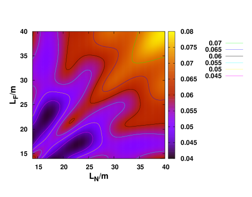
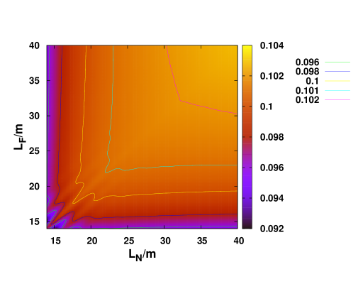
Figure 1: The sensitivity to sin22θ14superscript22subscript𝜃14\sin^{2}2\theta_{14} as a function of the two baseline lengths in the case of an ordinary thermal neutron reactor of a diameter 4m, a height 4m, a thermal power 2.8GW. Δm412=1Δsubscriptsuperscript𝑚2411\Delta m^{2}_{41}=1eV2 (upper panel), 5eV2 (lower) is assumed.
Refer to caption
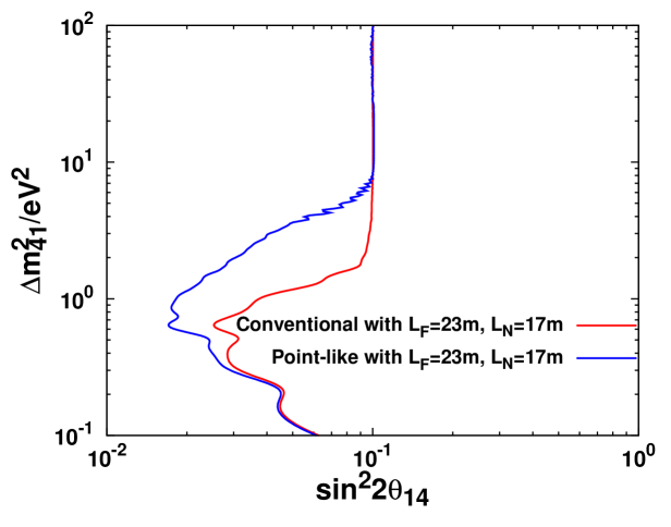
Figure 2: The sensitivity to sin22θ14superscript22subscript𝜃14\sin^{2}2\theta_{14}. The red line stands for the one for a thermal neutron reactor (of a diameter 4m, a height 4m, a thermal power 2.8GW) with two detectors at LF=23subscript𝐿𝐹23L_{F}=23m and LN=17subscript𝐿𝑁17L_{N}=17m, while the blue line for the one for a hypothetical reactor with a point-like core.

III.2 Thermal neutron reactors

A core of conventional (thermal neutron) reactors typically has a diameter of 4m, a height 4m and its thermal power is typically a few GW. As we will see below, when we try to perform an oscillation experiment at very short baseline lengths, smearing of the reactor core size gives a nontrivial contribution to the results because the baseline lengths are comparable to the core size.

We have computed χ2superscript𝜒2\chi^{2} in Eq. (3) numerically in the case of a thermal neutron reactor. Fig. 1 shows the sensitivity to sin22θ14superscript22subscript𝜃14\sin^{2}{2\theta_{14}} as a function of the baseline lengths of the near and far detectors for Δm412=1Δsubscriptsuperscript𝑚2411\Delta m^{2}_{41}=1eV2, and 5eV2, respectively. We have assumed a thermal power of 2.8GW, and a diameter of 4m and a height of 4m, and we have varied the baseline lengths in the range 14mLAless-than-or-similar-toabsentsubscript𝐿𝐴less-than-or-similar-toabsent\lesssim L_{A}\lesssim40m. Unlike the case of infinite statistics Sugiyama:2005ir , the statistical errors are important in the present setup of the detectors, and longer baseline lengths are disfavored.

For Δm412=1Δsubscriptsuperscript𝑚2411\Delta m^{2}_{41}=1eV2 (Fig. 1 upper panel), the set (LN,LF)similar-to-or-equalssubscript𝐿𝑁subscript𝐿𝐹absent(L_{N},L_{F})\simeq (17m, 23m) gives the optimum. In contrast to the rate analysis, in which the optimized baseline length of the near detector is LNsubscript𝐿𝑁L_{N}=0m to avoid oscillations, the spectrum analysis with (LN,LF)=subscript𝐿𝑁subscript𝐿𝐹absent(L_{N},L_{F})= (17m, 23m) looks at the difference between the maximum and minimum of the spectrum shape with neutrino oscillations at LNsubscript𝐿𝑁L_{N} and LFsubscript𝐿𝐹L_{F} mainly for the energy region Eνsimilar-tosubscript𝐸𝜈absentE_{\nu}\sim 4MeV where the number of events are expected to be the largest.

On the other hand, for Δm412=5Δsubscriptsuperscript𝑚2415\Delta m^{2}_{41}=5eV2 (Fig. 1 lower panel), the sensitivity to sin22θ14superscript22subscript𝜃14\sin^{2}{2\theta_{14}} is as low as 0.1 for most of the set of the baseline lengths (LN,LF)subscript𝐿𝑁subscript𝐿𝐹(L_{N},L_{F}). This implies that Δm412Δsubscriptsuperscript𝑚241\Delta m^{2}_{41} is so large that we have average over rapid oscillations for almost any baseline lengths and the only term which contributes in Eq. (8) is the first term, that corresponds to the rate analysis.

Fig. 2 shows the sensitivity to sin22θ14superscript22subscript𝜃14\sin^{2}{2\theta_{14}} as a function of Δm412Δsubscriptsuperscript𝑚241\Delta m^{2}_{41} in the case of the baseline lengths (LN,LF)=subscript𝐿𝑁subscript𝐿𝐹absent(L_{N},L_{F})= (17m, 23m). For Δm4122greater-than-or-equivalent-toΔsubscriptsuperscript𝑚2412\Delta m^{2}_{41}\gtrsim 2eV2, it indicates that the sensitivity is no better than 0.1, which is basically the result of the rate analysis. The sensitivity in the case of a hypothetical point-like reactor, where all the conditions for the detectors are the same, is also given in Fig. 2 for comparison. Fig. 2 indicates that the sensitivity would be as good as several ×102absentsuperscript102\times 10^{-2} for a few eV2, if the core were point-like. So we can conclude that we have poor sensitivity for Δm412greater-than-or-equivalent-toΔsubscriptsuperscript𝑚241absent\Delta m^{2}_{41}\gtrsim 2eV2 because of the smearing effect of the finite core size of the reactor. We have computed the sensitivity also for different numbers of bins (n𝑛n=16, 64), and verified explicitly that the result of Fig. 2 is almost independent of n𝑛n for 16n6416𝑛6416\leq n\leq 64. This is because the statistical errors are dominant in χ2superscript𝜒2\chi^{2}.

Refer to caption
Refer to caption
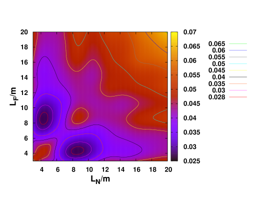
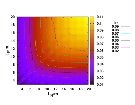
Figure 3: The sensitivity to sin22θ14superscript22subscript𝜃14\sin^{2}2\theta_{14} as a function of the two baseline lengths in the case of Joyo joyo with MK-III upgrade joyomk3 which is an experimental fast reactor (of a diameter 0.8m, a height 0.5m, a thermal power 0.14GW). Δm412=1Δsubscriptsuperscript𝑚2411\Delta m^{2}_{41}=1eV2 (upper panel), 5eV2 (lower) is assumed.
Refer to caption
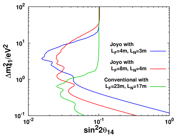
Figure 4: The sensitivity to sin22θ14superscript22subscript𝜃14\sin^{2}2\theta_{14} of the Joyo reactor with two detectors. The Blue line stands for the one in the case with two detectors at LF=4subscript𝐿𝐹4L_{F}=4m and LN=3subscript𝐿𝑁3L_{N}=3m, while the red line for the one for in the case with two detectors at LF=8subscript𝐿𝐹8L_{F}=8m and LN=4subscript𝐿𝑁4L_{N}=4m. The sensitivity in the case of a conventional thermal neutron reactor (the green line) is also given for comparison.

III.3 Experimental fast neutron reactors

In the previous subsection, we have seen that the sensitivity to sin22θ14superscript22subscript𝜃14\sin^{2}{2\theta_{14}} is lost because of the smearing effect of finite core size. Fast neutron reactors are known to have a high power density, and an oscillation experiments using them might be more advantageous than those with thermal neutron reactors. While experimental fast neutron reactors have a small power, it may allow experimentalists to put the detectors at a nearer location because of their experimental nature.

Here we will discuss the concrete example of Joyo joyo with MK-III upgrade joyomk3 , which is an experimental fast breeder reactor.777 An experiment Furuta:2011iu was performed to detect neutrinos from a fast neutron reactor at Joyo, although they did not get sufficient statistical significance. It has a relatively small size (a diameter of 0.8m, a height of 0.5m), and a relatively large thermal power 0.14GW. Its power density is approximately 500 kW/\ell, whereas a typical power density of thermal neutron reactors is approximately 50 kW/\ell.

Again we have computed χ2superscript𝜒2\chi^{2} in Eq. (3) numerically in the case of Joyo with MK-III upgrade. Fig. 3 shows the sensitivity to sin22θ14superscript22subscript𝜃14\sin^{2}{2\theta_{14}} as a function of the baseline lengths of the near and far detectors for Δm412=1Δsubscriptsuperscript𝑚2411\Delta m^{2}_{41}=1eV2, and 5eV2, respectively. We have assumed the same conditions for the detectors (the size, the efficiency, the exposure time etc.) as those assumed in Fig. 1. From Fig. 3 we see that the set (LN,LF)similar-to-or-equalssubscript𝐿𝑁subscript𝐿𝐹absent(L_{N},L_{F})\simeq (4m, 8m) gives the optimum for Δm412=1Δsubscriptsuperscript𝑚2411\Delta m^{2}_{41}=1eV2 (Fig. 3 upper panel).

Fig. 4 shows the sensitivity to sin22θ14superscript22subscript𝜃14\sin^{2}{2\theta_{14}} as a function of Δm412Δsubscriptsuperscript𝑚241\Delta m^{2}_{41} in the case of the sets of the baseline lengths (LN,LF)=subscript𝐿𝑁subscript𝐿𝐹absent(L_{N},L_{F})= (4m, 8m) and (LN,LF)=subscript𝐿𝑁subscript𝐿𝐹absent(L_{N},L_{F})= (3m, 4m). The set of the baseline lengths (LN,LF)=subscript𝐿𝑁subscript𝐿𝐹absent(L_{N},L_{F})= (3m, 4m) has a peak for sin22θ14similar-to-or-equalssuperscript22subscript𝜃14absent\sin^{2}{2\theta_{14}}\simeq 4 eV2, while the other set (LN,LF)=subscript𝐿𝑁subscript𝐿𝐹absent(L_{N},L_{F})= (4m, 8m) has sensitivity to sin22θ14superscript22subscript𝜃14\sin^{2}{2\theta_{14}} for a wider range of Δm412Δsubscriptsuperscript𝑚241\Delta m^{2}_{41}. The sensitivity in the case of a conventional thermal neutron reactor is also given in Fig. 2 for comparison, and the advantage of the case with Joyo is clear. Also in this case the statistical errors are dominant in χ2superscript𝜒2\chi^{2}, and the result of Fig. 4 is almost independent of the number n𝑛n of bins for 16n6416𝑛6416\leq n\leq 64.

IV Discussion and Conclusion

In the framework of the (3+1)-scheme, we studied the sensitivity to sin22θ14superscript22subscript𝜃14\sin^{2}2\theta_{14} of very short baseline reactor oscillation experiments by a spectrum analysis. The assumptions are that we have two detectors whose size and efficiency are exactly the same as those used at the Bugey experiment Declais:1994su .

In the case of a conventional thermal neutron reactor, which has a core of a diameter 4m, a height 4m and a thermal power 2.8GW, by putting the detectors at LN=subscript𝐿𝑁absentL_{N}= 17m and LF=subscript𝐿𝐹absentL_{F}= 23m, we obtain the sensitivity as good as several ×102absentsuperscript102\times 10^{-2} for Δm4121less-than-or-similar-toΔsubscriptsuperscript𝑚2411\Delta m^{2}_{41}\lesssim 1eV2, but we lose the sensitivity above 1eV2 due to the smearing of the finite core size.

In the case of an experimental fast neutron reactor with a core of a diameter of 0.8m, a height of 0.5m and a thermal power 0.14GW, on the other hand, we obtain the sensitivity as good as a several ×102absentsuperscript102\times 10^{-2} for 1eV2 Δm41210less-than-or-similar-toabsentΔsubscriptsuperscript𝑚241less-than-or-similar-to10\lesssim\Delta m^{2}_{41}\lesssim 10eV2 if we put the detectors at LN=subscript𝐿𝑁absentL_{N}= 4m and LF=subscript𝐿𝐹absentL_{F}= 8m.

In both types of reactors with the Bugey-like detector setup, the statistical errors are dominant, and the sensitivity is almost independent of the number n𝑛n of bins of the spectral analysis. The reason that the case of the experimental fast neutron reactor is competitive despite its small power is because the total numbers of events at Lsimilar-to𝐿absentL\sim several meters are comparable to those of the case with the thermal neutron reactor at Lsimilar-to𝐿absentL\sim a few ×\times 10 meters.

Since the best fit value obtained in Ref. Mention:2011rk is Δm4122similar-toΔsubscriptsuperscript𝑚2412\Delta m^{2}_{41}\sim 2eV2, an experiment using an experimental fast neutron reactor offers a promising possibility.

It should be emphasized that the flux uncertainty by 3% which was pointed out in Ref. Mueller:2011nm does not cause a problem in our discussion. The reason is because the main contribution to χ2superscript𝜒2\chi^{2} comes from the spectrum analysis, which looks at the difference of the maximum and the minimum of the energy spectrum and the effect of the overall normalization of the flux (the first term of the RHS in Eq. (8)) gives little contribution to χ2superscript𝜒2\chi^{2} in the region of Δm412Δsubscriptsuperscript𝑚241\Delta m^{2}_{41} in which the sensitivity to sin22θ14superscript22subscript𝜃14\sin^{2}2\theta_{14} is better than 0.1.

Although we may not be able to put the detectors at such a close location, we could increase the detector volume and/or the measurement period, so that the data size is the same as those described in this paper. While the experimental feasibility of the idea of putting detectors at a location very near to an experimental fast reactor is yet to be seen, it is worth investigating whether this method is technically possible.

Appendix A Derivation of the covariance matrix

By choosing the bins in such a way that tiA=tAsubscriptsuperscript𝑡𝐴𝑖superscript𝑡𝐴t^{A}_{i}=t^{A}, Eq. (3) becomes

χ2superscript𝜒2\displaystyle\displaystyle\chi^{2} =\displaystyle= minαs{A=N,Fi=1n(miA/tiA1ααAαiαcalAviA)21/tA+(σdbA)2\displaystyle\min_{\alpha^{\prime}s}\Bigg{\{}\displaystyle\sum_{A=N,F}\sum_{i=1}^{n}\frac{\left(m^{A}_{i}/t^{A}_{i}-1-\alpha-\alpha^{A}-\alpha_{i}-\alpha_{\text{cal}}^{A}v^{A}_{i}\right)^{2}}{1/t^{A}+(\sigma^{A}_{\text{db}})^{2}}
+\displaystyle+ A=N,F[(αAσdB)2+(αcalAσcal)2]+i=1n(αiσDb)2+(ασDB)2}\displaystyle\displaystyle\sum_{A=N,F}\left[\left(\frac{\alpha^{A}}{\sigma_{\text{dB}}}\right)^{2}+\left(\frac{\alpha_{\text{cal}}^{A}}{\sigma_{\text{cal}}}\right)^{2}\right]+\displaystyle\sum_{i=1}^{n}\left(\frac{\alpha_{i}}{\sigma_{\text{Db}}}\right)^{2}+\left(\frac{\alpha}{\sigma_{\text{DB}}}\right)^{2}\Bigg{\}}
\displaystyle\equiv minαsχα2.subscriptsuperscript𝛼𝑠subscriptsuperscript𝜒2𝛼\displaystyle\min_{\alpha^{\prime}s}\chi^{2}_{\alpha}.

Let us redefine the variables

yiAsubscriptsuperscript𝑦𝐴𝑖\displaystyle y^{A}_{i} \displaystyle\equiv miAtiAtiA=sin22θ14DiAsubscriptsuperscript𝑚𝐴𝑖subscriptsuperscript𝑡𝐴𝑖subscriptsuperscript𝑡𝐴𝑖superscript22subscript𝜃14subscriptsuperscript𝐷𝐴𝑖\displaystyle\frac{m^{A}_{i}-t^{A}_{i}}{t^{A}_{i}}=-\sin^{2}2\theta_{14}D^{A}_{i}

and let us introduce a vector notation

yN(y1NynN),yF(y1FynF).formulae-sequencesuperscript𝑦𝑁subscriptsuperscript𝑦𝑁1subscriptsuperscript𝑦𝑁𝑛superscript𝑦𝐹subscriptsuperscript𝑦𝐹1subscriptsuperscript𝑦𝐹𝑛\displaystyle\vec{y}^{N}\equiv\left(\begin{array}[]{c}y^{N}_{1}\\ \vdots\\ y^{N}_{n}\end{array}\right),\qquad\vec{y}^{F}\equiv\left(\begin{array}[]{c}y^{F}_{1}\\ \vdots\\ y^{F}_{n}\end{array}\right). (16)

Following the discussions in the Appendix A in Sugiyama:2004bv , the matrix element of the covariance matrix can be obtained as the expectation value of yiAyjBsubscriptsuperscript𝑦𝐴𝑖subscriptsuperscript𝑦𝐵𝑗y^{A}_{i}\,y^{B}_{j}:

(ρ)ijABsubscriptsuperscript𝜌𝐴𝐵𝑖𝑗\displaystyle\left(\rho\right)^{AB}_{ij} =\displaystyle= yiAyjBdelimited-⟨⟩subscriptsuperscript𝑦𝐴𝑖subscriptsuperscript𝑦𝐵𝑗\displaystyle\left\langle y^{A}_{i}y^{B}_{j}\right\rangle
\displaystyle\equiv 𝒩𝑑αA=N,F𝑑yA𝑑αA𝑑αcalAi=1n𝑑αiyiAyjBexp(χα22),𝒩differential-d𝛼subscriptproduct𝐴𝑁𝐹differential-dsuperscript𝑦𝐴differential-dsuperscript𝛼𝐴differential-dsuperscriptsubscript𝛼cal𝐴superscriptsubscriptproduct𝑖1𝑛differential-dsubscript𝛼𝑖subscriptsuperscript𝑦𝐴𝑖subscriptsuperscript𝑦𝐵𝑗subscriptsuperscript𝜒2𝛼2\displaystyle{\cal N}\int d\alpha\prod_{A=N,F}\int d\vec{y}^{A}\int d\alpha^{A}\int d\alpha_{\text{cal}}^{A}\prod_{i=1}^{n}\int d\alpha_{i}~{}y^{A}_{i}\,y^{B}_{j}\,\exp\left(-\frac{\chi^{2}_{\alpha}}{2}\right),

where the normalization 𝒩𝒩{\cal N} is defined in such a way that 1=1delimited-⟨⟩11\langle 1\rangle=1. From a straightforward calculation, we have

yiAyjBdelimited-⟨⟩subscriptsuperscript𝑦𝐴𝑖subscriptsuperscript𝑦𝐵𝑗\displaystyle\left\langle y^{A}_{i}y^{B}_{j}\right\rangle =\displaystyle= δABδij1/tA+δABδijσdb2+σDB2+δABσdB2+δijσDb2+δABviAvjAσcal2.superscript𝛿𝐴𝐵subscript𝛿𝑖𝑗1superscript𝑡𝐴superscript𝛿𝐴𝐵subscript𝛿𝑖𝑗superscriptsubscript𝜎db2superscriptsubscript𝜎DB2superscript𝛿𝐴𝐵superscriptsubscript𝜎dB2subscript𝛿𝑖𝑗superscriptsubscript𝜎Db2superscript𝛿𝐴𝐵subscriptsuperscript𝑣𝐴𝑖subscriptsuperscript𝑣𝐴𝑗subscriptsuperscript𝜎2cal\displaystyle\delta^{AB}\delta_{ij}1/t^{A}+\delta^{AB}\delta_{ij}\,\sigma_{\text{db}}^{2}+\sigma_{\text{DB}}^{2}+\delta^{AB}\,\sigma_{\text{dB}}^{2}+\delta_{ij}\,\sigma_{\text{Db}}^{2}+\delta^{AB}v^{A}_{i}v^{A}_{j}\,\sigma^{2}_{\text{cal}}.

Thus we have

χ2=(yNT,yFT)ρ1(yNyF)=sin42θ14(DNT,DFT)ρ1(DNDF),superscript𝜒2superscript𝑦𝑁𝑇superscript𝑦𝐹𝑇superscript𝜌1superscript𝑦𝑁superscript𝑦𝐹superscript42subscript𝜃14superscript𝐷𝑁𝑇superscript𝐷𝐹𝑇superscript𝜌1superscript𝐷𝑁superscript𝐷𝐹\displaystyle\displaystyle\chi^{2}=\left(\begin{array}[]{ll}\vec{y}^{N\ T},&\vec{y}^{F\ T}\end{array}\right)\rho^{-1}\left(\begin{array}[]{l}\vec{y}^{N}\\ \vec{y}^{F}\end{array}\right)=\sin^{4}2\theta_{14}\left(\begin{array}[]{ll}\vec{D}^{N\ T},&\vec{D}^{F\ T}\end{array}\right)\rho^{-1}\left(\begin{array}[]{l}\vec{D}^{N}\\ \vec{D}^{F}\end{array}\right), (23)

where the covariance matrix ρ𝜌\rho is defined by

ρ=(M+1/tNInNNM+1/tFIn),𝜌𝑀1superscript𝑡𝑁subscript𝐼𝑛𝑁𝑁𝑀1superscript𝑡𝐹subscript𝐼𝑛\displaystyle\rho=\left(\begin{array}[]{ll}M+1/t^{N}I_{n}&N\\ N&M+1/t^{F}I_{n}\end{array}\right), (26)

with

M𝑀\displaystyle M \displaystyle\equiv (σDb2+σdb2)In+(σDB2+σdB2)Hn+σcal2Gn,subscriptsuperscript𝜎2Dbsubscriptsuperscript𝜎2dbsubscript𝐼𝑛subscriptsuperscript𝜎2DBsubscriptsuperscript𝜎2dBsubscript𝐻𝑛subscriptsuperscript𝜎2calsubscript𝐺𝑛\displaystyle\left(\sigma^{2}_{\text{Db}}+\sigma^{2}_{\text{db}}\right)I_{n}+\left(\sigma^{2}_{\text{DB}}+\sigma^{2}_{\text{dB}}\right)H_{n}+\sigma^{2}_{\text{cal}}G_{n},
N𝑁\displaystyle N \displaystyle\equiv σDb2In+σDB2Hn.subscriptsuperscript𝜎2Dbsubscript𝐼𝑛subscriptsuperscript𝜎2DBsubscript𝐻𝑛\displaystyle\sigma^{2}_{\text{Db}}I_{n}+\sigma^{2}_{\text{DB}}H_{n}. (27)

Here Insubscript𝐼𝑛I_{n} is an n×n𝑛𝑛n\times n unit matrix, Hnsubscript𝐻𝑛H_{n} and Gnsubscript𝐺𝑛G_{n} are n×n𝑛𝑛n\times n matrices defined by

Hnsubscript𝐻𝑛\displaystyle H_{n} \displaystyle\equiv (1111),11missing-subexpression11\displaystyle\left(\begin{array}[]{ccc}1&\cdots&1\\ \vdots&&\vdots\\ 1&\cdots&1\end{array}\right), (31)
Gnsubscript𝐺𝑛\displaystyle G_{n} \displaystyle\equiv (v12v1v2v1vnv1v2v22v2vnv1vnv2vnvn2),superscriptsubscript𝑣12subscript𝑣1subscript𝑣2subscript𝑣1subscript𝑣𝑛subscript𝑣1subscript𝑣2superscriptsubscript𝑣22subscript𝑣2subscript𝑣𝑛missing-subexpressionsubscript𝑣1subscript𝑣𝑛subscript𝑣2subscript𝑣𝑛superscriptsubscript𝑣𝑛2\displaystyle\left(\begin{array}[]{cccc}v_{1}^{2}&v_{1}v_{2}&\cdots&v_{1}v_{n}\\ v_{1}v_{2}&v_{2}^{2}&\cdots&v_{2}v_{n}\\ \vdots&\vdots&&\vdots\\ v_{1}v_{n}&v_{2}v_{n}&\cdots&v_{n}^{2}\end{array}\right), (36)

where vj(j=1,,n)subscript𝑣𝑗𝑗1𝑛v_{j}~{}(j=1,\cdots,n) is defined by Eqs. (4), and (6). Note that the covariance matrix does not include oscillation parameters but only errors. Diagonalization of the covariance matrix is useful to see which errors dominate χ2superscript𝜒2\chi^{2}.

Unlike in Ref. Sugiyama:2005ir , the presence of the statistical errors 1/tA1superscript𝑡𝐴1/t^{A} and the matrix Gnsubscript𝐺𝑛G_{n} makes it difficult to evaluate the eigenvalues analytically, so only in this appendix, we will take the limit σcal20subscriptsuperscript𝜎2cal0\sigma^{2}_{\text{cal}}\to 0 which may be justified in the present setup with the total numbers of events similar-to\sim 10,000 ×(15m/LA)2absentsuperscript15msubscript𝐿𝐴2\times(15\mbox{m}/L_{A})^{2}.

To diagonalize the matrix (26) with σcal2=0subscriptsuperscript𝜎2cal0\sigma^{2}_{\text{cal}}=0, we first note that the matrix Hnsubscript𝐻𝑛H_{n} can be diagonalized as

Hn=UnDnUn1,subscript𝐻𝑛subscript𝑈𝑛subscript𝐷𝑛superscriptsubscript𝑈𝑛1\displaystyle H_{n}=U_{n}\,D_{n}\,U_{n}^{-1},

where

Dn=diag(n,0,,0)subscript𝐷𝑛diag𝑛00\displaystyle D_{n}=\mbox{\rm diag}(n,0,\cdots,0)

is a diagonal matrix and

Unsubscript𝑈𝑛\displaystyle U_{n} =\displaystyle= (u1,,un),subscript𝑢1subscript𝑢𝑛\displaystyle(\vec{u}_{1},\cdots,\vec{u}_{n}),
u1subscript𝑢1\displaystyle\vec{u}_{1} \displaystyle\equiv 1n(1,,1)T1𝑛superscript11𝑇\displaystyle\frac{1}{\sqrt{n}}\,(1,\cdots,1)^{T}
u2subscript𝑢2\displaystyle\vec{u}_{2} \displaystyle\equiv 12(1,1,0,,0)T12superscript1100𝑇\displaystyle\frac{1}{\sqrt{2}}\,(1,-1,0,\cdots,0)^{T}
u3subscript𝑢3\displaystyle\vec{u}_{3} \displaystyle\equiv 16(1,1,2,0,,0)T16superscript11200𝑇\displaystyle\frac{1}{\sqrt{6}}\,(1,1,-2,0,\cdots,0)^{T}
\displaystyle\cdots
unsubscript𝑢𝑛\displaystyle\vec{u}_{n} \displaystyle\equiv 1n(n1)(1,,1,(n1))T1𝑛𝑛1superscript11𝑛1𝑇\displaystyle\frac{1}{\sqrt{n(n-1)}}\,(1,\cdots,1,-(n-1))^{T}

is a n×n𝑛𝑛n\times n unitary matrix. Thus M𝑀M and N𝑁N can be diagonalized as

M𝑀\displaystyle M =\displaystyle= Un{(σDb2+σdb2)In+(σDB2+σdB2)Dn}Un1subscript𝑈𝑛subscriptsuperscript𝜎2Dbsubscriptsuperscript𝜎2dbsubscript𝐼𝑛subscriptsuperscript𝜎2DBsubscriptsuperscript𝜎2dBsubscript𝐷𝑛superscriptsubscript𝑈𝑛1\displaystyle U_{n}\,\left\{\left(\sigma^{2}_{\text{Db}}+\sigma^{2}_{\text{db}}\right)I_{n}+\left(\sigma^{2}_{\text{DB}}+\sigma^{2}_{\text{dB}}\right)D_{n}\right\}\,U_{n}^{-1}
=\displaystyle= Undiag(p1,p2,,p2)Un1,subscript𝑈𝑛diagsubscript𝑝1subscript𝑝2subscript𝑝2superscriptsubscript𝑈𝑛1\displaystyle U_{n}\,\mbox{\rm diag}(p_{1},p_{2},\cdots,p_{2})\,U_{n}^{-1},
N𝑁\displaystyle N =\displaystyle= Un(σDb2In+σDB2Dn)Un1subscript𝑈𝑛subscriptsuperscript𝜎2Dbsubscript𝐼𝑛subscriptsuperscript𝜎2DBsubscript𝐷𝑛superscriptsubscript𝑈𝑛1\displaystyle U_{n}\,\left(\sigma^{2}_{\text{Db}}I_{n}+\sigma^{2}_{\text{DB}}D_{n}\right)\,U_{n}^{-1}
=\displaystyle= Undiag(q1,q2,,q2)Un1,subscript𝑈𝑛diagsubscript𝑞1subscript𝑞2subscript𝑞2superscriptsubscript𝑈𝑛1\displaystyle U_{n}\,\mbox{\rm diag}(q_{1},q_{2},\cdots,q_{2})\,U_{n}^{-1},

where

p1subscript𝑝1\displaystyle p_{1} \displaystyle\equiv σDb2+σdb2+n(σDB2+σdB2)subscriptsuperscript𝜎2Dbsubscriptsuperscript𝜎2db𝑛subscriptsuperscript𝜎2DBsubscriptsuperscript𝜎2dB\displaystyle\sigma^{2}_{\text{Db}}+\sigma^{2}_{\text{db}}+n(\sigma^{2}_{\text{DB}}+\sigma^{2}_{\text{dB}})
p2subscript𝑝2\displaystyle p_{2} \displaystyle\equiv σDb2+σdb2subscriptsuperscript𝜎2Dbsubscriptsuperscript𝜎2db\displaystyle\sigma^{2}_{\text{Db}}+\sigma^{2}_{\text{db}}
q1subscript𝑞1\displaystyle q_{1} \displaystyle\equiv σDb2+nσDB2subscriptsuperscript𝜎2Db𝑛subscriptsuperscript𝜎2DB\displaystyle\sigma^{2}_{\text{Db}}+n\sigma^{2}_{\text{DB}}
q2subscript𝑞2\displaystyle q_{2} \displaystyle\equiv σDb2.subscriptsuperscript𝜎2Db\displaystyle\sigma^{2}_{\text{Db}}. (37)

Now (26) can be cast into a block diagonal by

(Un100Un1)(M+1/tNInNNM+1/tFIn)(Un00Un)superscriptsubscript𝑈𝑛100superscriptsubscript𝑈𝑛1𝑀1superscript𝑡𝑁subscript𝐼𝑛𝑁𝑁𝑀1superscript𝑡𝐹subscript𝐼𝑛subscript𝑈𝑛00subscript𝑈𝑛\displaystyle\left(\begin{array}[]{cc}U_{n}^{-1}&0\\ 0&U_{n}^{-1}\end{array}\right)\left(\begin{array}[]{cc}M+1/t^{N}I_{n}&N\\ N&M+1/t^{F}I_{n}\end{array}\right)\left(\begin{array}[]{cc}U_{n}&0\\ 0&U_{n}\end{array}\right) (44)
=\displaystyle= ((σDb2+σdb2+1/tN)In+(σDB2+σdB2)DnσDb2In+σDB2DnσDb2In+σDB2Dn(σDb2+σdb2+1/tF)In+(σDB2+σdB2)Dn)subscriptsuperscript𝜎2Dbsubscriptsuperscript𝜎2db1superscript𝑡𝑁subscript𝐼𝑛subscriptsuperscript𝜎2DBsubscriptsuperscript𝜎2dBsubscript𝐷𝑛subscriptsuperscript𝜎2Dbsubscript𝐼𝑛subscriptsuperscript𝜎2DBsubscript𝐷𝑛subscriptsuperscript𝜎2Dbsubscript𝐼𝑛subscriptsuperscript𝜎2DBsubscript𝐷𝑛subscriptsuperscript𝜎2Dbsubscriptsuperscript𝜎2db1superscript𝑡𝐹subscript𝐼𝑛subscriptsuperscript𝜎2DBsubscriptsuperscript𝜎2dBsubscript𝐷𝑛\displaystyle\left(\begin{array}[]{cc}\left(\sigma^{2}_{\text{Db}}+\sigma^{2}_{\text{db}}+1/t^{N}\right)I_{n}+\left(\sigma^{2}_{\text{DB}}+\sigma^{2}_{\text{dB}}\right)D_{n}&\sigma^{2}_{\text{Db}}I_{n}+\sigma^{2}_{\text{DB}}D_{n}\\ \sigma^{2}_{\text{Db}}I_{n}+\sigma^{2}_{\text{DB}}D_{n}&\left(\sigma^{2}_{\text{Db}}+\sigma^{2}_{\text{db}}+1/t^{F}\right)I_{n}+\left(\sigma^{2}_{\text{DB}}+\sigma^{2}_{\text{dB}}\right)D_{n}\end{array}\right) (47)
=\displaystyle= 𝒰(B1000B2000B2)𝒰T,𝒰subscript𝐵10missing-subexpression00subscript𝐵2missing-subexpressionmissing-subexpression000missing-subexpressionsubscript𝐵2superscript𝒰𝑇\displaystyle{\cal U}\left(\begin{array}[]{ccccc}B_{1}&0&\cdots&&0\\ 0&B_{2}&\ddots&&\vdots\\ \vdots&\ddots&\ddots&&0\\ 0&\cdots&0&&B_{2}\end{array}\right){\cal U}^{T}, (52)

where 𝒰𝒰{\cal U} is a 2n×2n2𝑛2𝑛2n\times 2n unitary matrix whose matrix elements are given by

𝒰pq(100000000100010000000010010000001)pq=j=1n(δp,2j1δq,j+δp,2jδq,n+j).subscript𝒰𝑝𝑞subscript1000000001000100000000100missing-subexpression1missing-subexpressionmissing-subexpression0000001𝑝𝑞superscriptsubscript𝑗1𝑛subscript𝛿𝑝2𝑗1subscript𝛿𝑞𝑗subscript𝛿𝑝2𝑗subscript𝛿𝑞𝑛𝑗\displaystyle{\cal U}_{pq}\equiv\left(\begin{array}[]{cccc|cccc}1&0&\cdots&0&0&0&\cdots&0\\ 0&0&\cdots&0&1&0&\cdots&0\\ 0&1&0&\cdots&0&0&\cdots&0\\ 0&0&\ddots&0&0&1&\cdots&0\\ 0&&\cdots&1&&&\ddots&0\\ 0&0&\cdots&0&0&\cdots&0&1\end{array}\right)_{pq}=\sum_{j=1}^{n}\left(\delta_{p,2j-1}\delta_{q,j}+\delta_{p,2j}\delta_{q,n+j}\right). (59)

B1subscript𝐵1B_{1}, B2subscript𝐵2B_{2} are 2×2222\times 2 matrices defined as follows and are diagonalized as

B1subscript𝐵1\displaystyle B_{1} \displaystyle\equiv (p1+1/tNq1q1p1+1/tF)=eiφ1σ2diag(λ1(),λ1(+))eiφ1σ2subscript𝑝11superscript𝑡𝑁subscript𝑞1subscript𝑞1subscript𝑝11superscript𝑡𝐹superscript𝑒𝑖subscript𝜑1subscript𝜎2diagsuperscriptsubscript𝜆1superscriptsubscript𝜆1superscript𝑒𝑖subscript𝜑1subscript𝜎2\displaystyle\left(\begin{array}[]{cc}p_{1}+1/t^{N}&q_{1}\\ q_{1}&p_{1}+1/t^{F}\end{array}\right)=e^{i\varphi_{1}\sigma_{2}}\,\mbox{\rm diag}(\lambda_{1}^{(-)},\lambda_{1}^{(+)})\,e^{-i\varphi_{1}\sigma_{2}} (62)
B2subscript𝐵2\displaystyle B_{2} \displaystyle\equiv (p2+1/tNq2q2p2+1/tF)=eiφ2σ2diag(λ2(),λ2(+))eiφ2σ2,subscript𝑝21superscript𝑡𝑁subscript𝑞2subscript𝑞2subscript𝑝21superscript𝑡𝐹superscript𝑒𝑖subscript𝜑2subscript𝜎2diagsuperscriptsubscript𝜆2superscriptsubscript𝜆2superscript𝑒𝑖subscript𝜑2subscript𝜎2\displaystyle\left(\begin{array}[]{cc}p_{2}+1/t^{N}&q_{2}\\ q_{2}&p_{2}+1/t^{F}\end{array}\right)=e^{i\varphi_{2}\sigma_{2}}\,\mbox{\rm diag}(\lambda_{2}^{(-)},\lambda_{2}^{(+)})\,e^{-i\varphi_{2}\sigma_{2}}, (65)

where

σ2(0ii0)subscript𝜎20𝑖𝑖0\displaystyle\sigma_{2}\equiv\left(\begin{array}[]{cc}0&-i\\ i&0\end{array}\right) (68)

is the Pauli matrix, φ1subscript𝜑1\varphi_{1} and φ2subscript𝜑2\varphi_{2} are introduced to diagonalize each matrix and are given by

tan2φ12subscript𝜑1\displaystyle\tan 2\varphi_{1} =\displaystyle= 2q11/tF1/tN=2(σDb2+nσDB2)1/tF1/tN2subscript𝑞11superscript𝑡𝐹1superscript𝑡𝑁2subscriptsuperscript𝜎2Db𝑛subscriptsuperscript𝜎2DB1superscript𝑡𝐹1superscript𝑡𝑁\displaystyle\frac{2q_{1}}{1/t^{F}-1/t^{N}}=\frac{2(\sigma^{2}_{\text{Db}}+n\sigma^{2}_{\text{DB}})}{1/t^{F}-1/t^{N}}
tan2φ22subscript𝜑2\displaystyle\tan 2\varphi_{2} =\displaystyle= 2q21/tF1/tN=2σDb21/tF1/tN,2subscript𝑞21superscript𝑡𝐹1superscript𝑡𝑁2subscriptsuperscript𝜎2Db1superscript𝑡𝐹1superscript𝑡𝑁\displaystyle\frac{2q_{2}}{1/t^{F}-1/t^{N}}=\frac{2\sigma^{2}_{\text{Db}}}{1/t^{F}-1/t^{N}}, (69)

and λj(±)(j=1,2)subscriptsuperscript𝜆plus-or-minus𝑗𝑗12\lambda^{(\pm)}_{j}~{}(j=1,2) are the eigenvalues given by

λ1(±)subscriptsuperscript𝜆plus-or-minus1\displaystyle\lambda^{(\pm)}_{1} \displaystyle\equiv n[σDb2+σdb2n+σDB2+σdB2+12(1NF+1NN)\displaystyle n\left[\frac{\sigma^{2}_{\text{Db}}+\sigma^{2}_{\text{db}}}{n}+\sigma^{2}_{\text{DB}}+\sigma^{2}_{\text{dB}}+\frac{1}{2}\left(\frac{1}{N^{F}}+\frac{1}{N^{N}}\right)\right.
±{14(1NF1NN)2+(σDb2n+σDB2)2}]\displaystyle\pm\left.\left\{\frac{1}{4}\left(\frac{1}{N^{F}}-\frac{1}{N^{N}}\right)^{2}+\left(\frac{\sigma^{2}_{\text{Db}}}{n}+\sigma^{2}_{\text{DB}}\right)^{2}\right\}\right]
λ2(±)subscriptsuperscript𝜆plus-or-minus2\displaystyle\lambda^{(\pm)}_{2} \displaystyle\equiv n[σDb2+σdb2n+12(1NF+1NN)\displaystyle n\left[\frac{\sigma^{2}_{\text{Db}}+\sigma^{2}_{\text{db}}}{n}+\frac{1}{2}\left(\frac{1}{N^{F}}+\frac{1}{N^{N}}\right)\right.
±{14(1NF1NN)2+(σDb2n)2}].\displaystyle\pm\left.\left\{\frac{1}{4}\left(\frac{1}{N^{F}}-\frac{1}{N^{N}}\right)^{2}+\left(\frac{\sigma^{2}_{\text{Db}}}{n}\right)^{2}\right\}\right].

In the last expression, we have factored out n𝑛n from the eigenvalues for later convenience, and we have introduced the total numbers of events NAn×tA(A=N,F)superscript𝑁𝐴𝑛superscript𝑡𝐴𝐴𝑁𝐹N^{A}\equiv n\times t^{A}~{}(A=N,F).

To evaluate χ2superscript𝜒2\chi^{2}, we need to calculate the following factor:

(eiφ1σ2000eiφ2σ200eiφ2σ2)𝒰(Un100Un1)(DNDF)superscript𝑒𝑖subscript𝜑1subscript𝜎2000superscript𝑒𝑖subscript𝜑2subscript𝜎20missing-subexpressionmissing-subexpressionmissing-subexpression0missing-subexpressionsuperscript𝑒𝑖subscript𝜑2subscript𝜎2𝒰superscriptsubscript𝑈𝑛100superscriptsubscript𝑈𝑛1superscript𝐷𝑁superscript𝐷𝐹\displaystyle\left(\begin{array}[]{cccc}e^{-i\varphi_{1}\sigma_{2}}&0&\cdots&0\\ 0&e^{-i\varphi_{2}\sigma_{2}}&\cdots&0\\ &&\ddots&\\ 0&\cdots&&e^{-i\varphi_{2}\sigma_{2}}\end{array}\right){\cal U}\left(\begin{array}[]{cc}U_{n}^{-1}&0\\ 0&U_{n}^{-1}\end{array}\right)\left(\begin{array}[]{c}\vec{D}^{N}\\ \vec{D}^{F}\end{array}\right) (78)
=\displaystyle= (eiφ1σ2000eiφ2σ200eiφ2σ2)𝒰(u1DNunDNu1DFunDF)superscript𝑒𝑖subscript𝜑1subscript𝜎2000superscript𝑒𝑖subscript𝜑2subscript𝜎20missing-subexpressionmissing-subexpressionmissing-subexpression0missing-subexpressionsuperscript𝑒𝑖subscript𝜑2subscript𝜎2𝒰subscript𝑢1superscript𝐷𝑁subscript𝑢𝑛superscript𝐷𝑁subscript𝑢1superscript𝐷𝐹subscript𝑢𝑛superscript𝐷𝐹\displaystyle\left(\begin{array}[]{cccc}e^{-i\varphi_{1}\sigma_{2}}&0&\cdots&0\\ 0&e^{-i\varphi_{2}\sigma_{2}}&\cdots&0\\ &&\ddots&\\ 0&\cdots&&e^{-i\varphi_{2}\sigma_{2}}\end{array}\right){\cal U}\left(\begin{array}[]{c}\vec{u}_{1}\cdot\vec{D}^{N}\\ \vdots\\ \vec{u}_{n}\cdot\vec{D}^{N}\\ \vec{u}_{1}\cdot\vec{D}^{F}\\ \vdots\\ \vec{u}_{n}\cdot\vec{D}^{F}\end{array}\right) (89)
=\displaystyle= (eiφ1σ2(u1DNu1DF)eiφ2σ2(u2DNu2DF)eiφ2σ2(unDNunDF))=((c1u1DNs1u1DFc1u1DF+s1u1DN)(c2u2DNs2u2DFc2u2DF+s2u2DN)(c2unDNs2unDFc2unDF+s2unDN)),superscript𝑒𝑖subscript𝜑1subscript𝜎2subscript𝑢1superscript𝐷𝑁subscript𝑢1superscript𝐷𝐹superscript𝑒𝑖subscript𝜑2subscript𝜎2subscript𝑢2superscript𝐷𝑁subscript𝑢2superscript𝐷𝐹superscript𝑒𝑖subscript𝜑2subscript𝜎2subscript𝑢𝑛superscript𝐷𝑁subscript𝑢𝑛superscript𝐷𝐹subscript𝑐1subscript𝑢1superscript𝐷𝑁subscript𝑠1subscript𝑢1superscript𝐷𝐹subscript𝑐1subscript𝑢1superscript𝐷𝐹subscript𝑠1subscript𝑢1superscript𝐷𝑁subscript𝑐2subscript𝑢2superscript𝐷𝑁subscript𝑠2subscript𝑢2superscript𝐷𝐹subscript𝑐2subscript𝑢2superscript𝐷𝐹subscript𝑠2subscript𝑢2superscript𝐷𝑁subscript𝑐2subscript𝑢𝑛superscript𝐷𝑁subscript𝑠2subscript𝑢𝑛superscript𝐷𝐹subscript𝑐2subscript𝑢𝑛superscript𝐷𝐹subscript𝑠2subscript𝑢𝑛superscript𝐷𝑁\displaystyle\left(\begin{array}[]{c}e^{-i\varphi_{1}\sigma_{2}}\left(\begin{array}[]{c}\vec{u}_{1}\cdot\vec{D}^{N}\\ \vec{u}_{1}\cdot\vec{D}^{F}\end{array}\right)\\ e^{-i\varphi_{2}\sigma_{2}}\left(\begin{array}[]{c}\vec{u}_{2}\cdot\vec{D}^{N}\\ \vec{u}_{2}\cdot\vec{D}^{F}\end{array}\right)\\ \vdots\\ e^{-i\varphi_{2}\sigma_{2}}\left(\begin{array}[]{c}\vec{u}_{n}\cdot\vec{D}^{N}\\ \vec{u}_{n}\cdot\vec{D}^{F}\end{array}\right)\end{array}\right)=\left(\begin{array}[]{c}\left(\begin{array}[]{c}c_{1}\vec{u}_{1}\cdot\vec{D}^{N}-s_{1}\vec{u}_{1}\cdot\vec{D}^{F}\\ c_{1}\vec{u}_{1}\cdot\vec{D}^{F}+s_{1}\vec{u}_{1}\cdot\vec{D}^{N}\end{array}\right)\\ \left(\begin{array}[]{c}c_{2}\vec{u}_{2}\cdot\vec{D}^{N}-s_{2}\vec{u}_{2}\cdot\vec{D}^{F}\\ c_{2}\vec{u}_{2}\cdot\vec{D}^{F}+s_{2}\vec{u}_{2}\cdot\vec{D}^{N}\end{array}\right)\\ \vdots\\ \left(\begin{array}[]{c}c_{2}\vec{u}_{n}\cdot\vec{D}^{N}-s_{2}\vec{u}_{n}\cdot\vec{D}^{F}\\ c_{2}\vec{u}_{n}\cdot\vec{D}^{F}+s_{2}\vec{u}_{n}\cdot\vec{D}^{N}\end{array}\right)\end{array}\right), (110)

where cjcosφj,sjsinφj(j=1,2)formulae-sequencesubscript𝑐𝑗subscript𝜑𝑗subscript𝑠𝑗subscript𝜑𝑗𝑗12c_{j}\equiv\cos\varphi_{j},s_{j}\equiv\sin\varphi_{j}~{}(j=1,2).

Putting everything together, we obtain

χ2sin42θ14superscript𝜒2superscript42subscript𝜃14\displaystyle\frac{\chi^{2}}{\sin^{4}2\theta_{14}} (111)
=\displaystyle= (c1u1DF+s1u1DN)2/nσDB2+σdB2+(σDb2+σdb2)/n+(1/NF+1/NN)/2+{(1/NF1/NN)2/4+(σDB2+σDb2/n)2}1/2superscriptsubscript𝑐1subscript𝑢1superscript𝐷𝐹subscript𝑠1subscript𝑢1superscript𝐷𝑁2𝑛subscriptsuperscript𝜎2DBsubscriptsuperscript𝜎2dBsubscriptsuperscript𝜎2Dbsubscriptsuperscript𝜎2db𝑛1superscript𝑁𝐹1superscript𝑁𝑁2superscriptsuperscript1superscript𝑁𝐹1superscript𝑁𝑁24superscriptsubscriptsuperscript𝜎2DBsubscriptsuperscript𝜎2Db𝑛212\displaystyle\frac{\left(c_{1}\vec{u}_{1}\cdot\vec{D}^{F}+s_{1}\vec{u}_{1}\cdot\vec{D}^{N}\right)^{2}/n}{\sigma^{2}_{\text{DB}}+\sigma^{2}_{\text{dB}}+(\sigma^{2}_{\text{Db}}+\sigma^{2}_{\text{db}})/n+(1/N^{F}+1/N^{N})/2+\left\{(1/N^{F}-1/N^{N})^{2}/4+(\sigma^{2}_{\text{DB}}+\sigma^{2}_{\text{Db}}/n)^{2}\right\}^{1/2}}
+(c1u1DNs1u1DF)2/nσDB2+σdB2+(σDb2+σdb2)/n+(1/NF+1/NN)/2{(1/NF1/NN)2/4+(σDB2+σDb2/n)2}1/2superscriptsubscript𝑐1subscript𝑢1superscript𝐷𝑁subscript𝑠1subscript𝑢1superscript𝐷𝐹2𝑛subscriptsuperscript𝜎2DBsubscriptsuperscript𝜎2dBsubscriptsuperscript𝜎2Dbsubscriptsuperscript𝜎2db𝑛1superscript𝑁𝐹1superscript𝑁𝑁2superscriptsuperscript1superscript𝑁𝐹1superscript𝑁𝑁24superscriptsubscriptsuperscript𝜎2DBsubscriptsuperscript𝜎2Db𝑛212\displaystyle+\frac{\left(c_{1}\vec{u}_{1}\cdot\vec{D}^{N}-s_{1}\vec{u}_{1}\cdot\vec{D}^{F}\right)^{2}/n}{\sigma^{2}_{\text{DB}}+\sigma^{2}_{\text{dB}}+(\sigma^{2}_{\text{Db}}+\sigma^{2}_{\text{db}})/n+(1/N^{F}+1/N^{N})/2-\left\{(1/N^{F}-1/N^{N})^{2}/4+(\sigma^{2}_{\text{DB}}+\sigma^{2}_{\text{Db}}/n)^{2}\right\}^{1/2}}
+j=2n(c2ujDF+s2ujDN)2/n(σDb2+σdb2)/n+(1/NF+1/NN)/2+{(1/NF1/NN)2/4+(σDb2/n)2}1/2superscriptsubscript𝑗2𝑛superscriptsubscript𝑐2subscript𝑢𝑗superscript𝐷𝐹subscript𝑠2subscript𝑢𝑗superscript𝐷𝑁2𝑛subscriptsuperscript𝜎2Dbsubscriptsuperscript𝜎2db𝑛1superscript𝑁𝐹1superscript𝑁𝑁2superscriptsuperscript1superscript𝑁𝐹1superscript𝑁𝑁24superscriptsubscriptsuperscript𝜎2Db𝑛212\displaystyle+\sum_{j=2}^{n}\frac{\left(c_{2}\vec{u}_{j}\cdot\vec{D}^{F}+s_{2}\vec{u}_{j}\cdot\vec{D}^{N}\right)^{2}/n}{(\sigma^{2}_{\text{Db}}+\sigma^{2}_{\text{db}})/n+(1/N^{F}+1/N^{N})/2+\left\{(1/N^{F}-1/N^{N})^{2}/4+(\sigma^{2}_{\text{Db}}/n)^{2}\right\}^{1/2}}
+j=2n(c2ujDNs2ujDF)2/n(σDb2+σdb2)/n+(1/NF+1/NN)/2{(1/NF1/NN)2/4+(σDb2/n)2}1/2,superscriptsubscript𝑗2𝑛superscriptsubscript𝑐2subscript𝑢𝑗superscript𝐷𝑁subscript𝑠2subscript𝑢𝑗superscript𝐷𝐹2𝑛subscriptsuperscript𝜎2Dbsubscriptsuperscript𝜎2db𝑛1superscript𝑁𝐹1superscript𝑁𝑁2superscriptsuperscript1superscript𝑁𝐹1superscript𝑁𝑁24superscriptsubscriptsuperscript𝜎2Db𝑛212\displaystyle+\sum_{j=2}^{n}\frac{\left(c_{2}\vec{u}_{j}\cdot\vec{D}^{N}-s_{2}\vec{u}_{j}\cdot\vec{D}^{F}\right)^{2}/n}{(\sigma^{2}_{\text{Db}}+\sigma^{2}_{\text{db}})/n+(1/N^{F}+1/N^{N})/2-\left\{(1/N^{F}-1/N^{N})^{2}/4+(\sigma^{2}_{\text{Db}}/n)^{2}\right\}^{1/2}},

where both the numerators and denominators are divided by the number n𝑛n of bins, because the numerators are almost independent of n𝑛n after being divided by n𝑛n in the limit of infinite statistics Sugiyama:2005ir .

In the present case, assuming that the total numbers of events NFsuperscript𝑁𝐹N^{F} and NNsuperscript𝑁𝑁N^{N} are of order 105superscript10510^{5} and that the number n𝑛n of bins is 32, our reference values (7) satisfy σDB29×1041/NA105(A=N,F)similar-to-or-equalssubscriptsuperscript𝜎2DB9superscript104much-greater-than1superscript𝑁𝐴similar-tosuperscript105𝐴𝑁𝐹\sigma^{2}_{\text{DB}}\simeq 9\times 10^{-4}\gg 1/N^{A}\sim 10^{-5}~{}(A=N,F), σdB23×105σdb2/n1×106similar-to-or-equalssubscriptsuperscript𝜎2dB3superscript105much-greater-thansubscriptsuperscript𝜎2db𝑛similar-to-or-equals1superscript106\sigma^{2}_{\text{dB}}\simeq 3\times 10^{-5}\gg\sigma^{2}_{\text{db}}/n\simeq 1\times 10^{-6}, σDb2/n1×1051/NA105(A=N,F)similar-to-or-equalssubscriptsuperscript𝜎2Db𝑛1superscript105similar-to1superscript𝑁𝐴similar-tosuperscript105𝐴𝑁𝐹\sigma^{2}_{\text{Db}}/n\simeq 1\times 10^{-5}\sim 1/N^{A}\sim 10^{-5}~{}(A=N,F). Hence we obtain Eq. (8).

Acknowledgements.
The author would like to thank F. Suekane for informing him of Ref. joyomk3 and for useful correspondence. This work was partly supported by Grants-in-Aid for Scientific Research of the Ministry of Education, Culture, Sports, Science, and Technology, under Grant No. 21540274.

References

  • (1) C. Athanassopoulos et al. [LSND Collaboration], Phys. Rev. Lett.  77 (1996) 3082 [arXiv:nucl-ex/9605003].
  • (2) C. Athanassopoulos et al. [LSND Collaboration], Phys. Rev. Lett.  81 (1998) 1774 [arXiv:nucl-ex/9709006].
  • (3) A. Aguilar et al. [LSND Collaboration], Phys. Rev.  D 64 (2001) 112007 [arXiv:hep-ex/0104049].
  • (4) K. Nakamura et al. [Particle Data Group], J. Phys. G 37 (2010) 075021.
  • (5) A. A. Aguilar-Arevalo et al. [The MiniBooNE Collaboration], Phys. Rev. Lett.  98 (2007) 231801 [arXiv:0704.1500 [hep-ex]].
  • (6) A. A. Aguilar-Arevalo et al. [The MiniBooNE Collaboration], Phys. Rev. Lett.  105 (2010) 181801 [arXiv:1007.1150 [hep-ex]].
  • (7) T. A. Mueller et al., Phys. Rev.  C 83 (2011) 054615 [arXiv:1101.2663 [hep-ex]].
  • (8) P. Huber, arXiv:1106.0687 [hep-ph].
  • (9) G. Mention, M. Fechner, T. Lasserre, T. A. Mueller, D. Lhuillier, M. Cribier a nd A. Letourneau, Phys. Rev.  D 83 (2011) 073006 [arXiv:1101.2755 [hep-ex]].
  • (10) Yu. Kozlov, L. Mikaelyan and V. Sinev, Phys. Atom. Nucl.  66 (2003) 469 [Yad. Fiz.  66 (2003) 497] [arXiv:hep-ph/0109277].
  • (11) H. Minakata, H. Sugiyama, O. Yasuda, K. Inoue and F. Suekane, Phys. Rev.  D 68 (2003) 033017 [Erratum-ibid.  D 70 (2004) 059901] [arXiv:hep-ph/0211111].
  • (12) P. Huber, M. Lindner, T. Schwetz and W. Winter, Nucl. Phys.  B 665 (2003) 487 [arXiv:hep-ph/0303232].
  • (13) K. Anderson et al., arXiv:hep-ex/0402041.
  • (14) F. Ardellier et al., arXiv:hep-ex/0405032.
  • (15) X. Guo et al. [Daya-Bay Collaboration], arXiv:hep-ex/0701029.
  • (16) J. K. Ahn et al. [RENO Collaboration], arXiv:1003.1391 [hep-ex].
  • (17) O. Yasuda, arXiv:hep-ph/0403162.
  • (18) H. Sugiyama, O. Yasuda, F. Suekane and G. A. Horton-Smith, Phys. Rev.  D 73 (2006) 053008 [arXiv:hep-ph/0409109].
  • (19) H. Sugiyama and O. Yasuda, Int. J. Mod. Phys.  A 22 (2007) 3407 [arXiv:hep-ph/0508090].
  • (20) J. Kopp, M. Maltoni and T. Schwetz, arXiv:1103.4570 [hep-ph].
  • (21) M. Sorel, J. M. Conrad and M. Shaevitz, Phys. Rev.  D 70 (2004) 073004 [arXiv:hep-ph/0305255].
  • (22) D. C. Latimer, J. Escamilla and D. J. Ernst, Phys. Rev.  C 75 (2007) 042501 [arXiv:hep-ex/0701004].
  • (23) A. de Gouvea and T. Wytock, Phys. Rev.  D 79 (2009) 073005 [arXiv:0809.5076 [hep-ph]].
  • (24) Y. Declais et al., Nucl. Phys.  B 434 (1995) 503.
  • (25) T. Lasserre [Nucifer Collaboration],
    http://www.e15.physik.tu-muenchen.de/fileadmin/downloads/seminars/
    1011/SterileNeutrinosWorkshop/lasserre-tumE15-feb2011-nucifer.pdf
    .
  • (26) C. Rubbia, talk at the 14th International Workshop on “Neutrino Telescopes”, Venice, Italy, March 15-18, 2011, http://agenda.infn.it/materialDisplay.py?contribId=34&
    sessionId=10&materialId=slides&confId=3101
    .
  • (27) S. K. Agarwalla, P. Huber and J. M. Link, JHEP 1001 (2010) 071 [arXiv:0907.3145 [hep-ph]].
  • (28) M. Cribier et al., arXiv:1107.2335 [hep-ex].
  • (29) M. Maltoni, T. Schwetz, M. A. Tortola and J. W. F. Valle, New J. Phys.  6 (2004) 122 [arXiv:hep-ph/0405172].
  • (30) N. Okada and O. Yasuda, Int. J. Mod. Phys.  A 12 (1997) 3669 [arXiv:hep-ph/9606411].
  • (31) S. M. Bilenky, C. Giunti and W. Grimus, Eur. Phys. J.  C 1 (1998) 247 [arXiv:hep-ph/9607372].
  • (32) F. Dydak et al., Phys. Lett.  B 134 (1984) 281.
  • (33) M. Maltoni and T. Schwetz, Phys. Rev.  D 76 (2007) 093005 [arXiv:0705.0107 [hep-ph]].
  • (34) The experimental fast reactor Joyo,
    http://www.jaea.go.jp/04/o-arai/joyo/english/index.html.
  • (35) T. Aoyama, T. Sekine, S. Maeda, A. Yoshida, Y. Maeda, S. Suzuki and T. Takeda, Nucl. Sci. Eng. 237, 353 (2007).
  • (36) H. Furuta et al., arXiv:1108.2910 [hep-ex].