Cosmological implications from the full shape of the large-scale power spectrum of the SDSS DR7 luminous red galaxies
Abstract
We obtain cosmological constraints from a measurement of the spherically averaged power spectrum of the distribution of about 90000 luminous red galaxies (LRGs) across 7646 deg2 in the Northern Galactic Cap from the seventh data release of the Sloan Digital Sky Survey. The errors and mode correlations are estimated thanks to the 160 LasDamas mock catalogues, created in order to simulate the same galaxies and to have the same selection as the data. We apply a model, that can accurately describe the full shape of the power spectrum with the use of a small number of free parameters. Using the LRG power spectrum, in combination with the latest measurement of the temperature and polarisation anisotropy in the cosmic microwave background (CMB), the luminosity-distance relation from the largest available type 1a supernovae (SNIa) dataset and a precise determination of the local Hubble parameter, we obtain cosmological constraints for five different parameter spaces. When all the four experiments are combined, the flat CDM model is characterised by , , , and . When we consider curvature as a free parameter, we do not detect deviations from flatness: , when only CMB and the LRG power spectrum are used; the inclusion of the other two experiments do not improve substantially this result. We also test for possible deviations from the cosmological constant paradigm. Considering the dark energy equation of state parameter as time independent, we measure , if the geometry is assumed to be flat, otherwise. When describing through a simple linear function of the scale factor, our results do not evidence any time evolution. In the next few years new experiments will allow to measure the clustering of galaxies with a precision much higher than achievable today. Models like the one used here will be a valuable tool in order to achieve the full potentials of the observations and obtain unbiased constraints on the cosmological parameters.
keywords:
large-scale structure of Universe – cosmology: theory – cosmology: observations – cosmological parameters1 Introduction
The last decade was characterised by a dramatic change in our vision of the Universe and by an impressive increase in size and quality of available datasets. At the end of the twentieth century, the analysis of the luminosity-distance relation in the Type 1a supernovae (SNIa) showed that the Universe is undergoing a phase of accelerated expansion driven by a new exotic component, dubbed dark energy, whose energy density is about 70% of the total (Riess et al., 1998; Perlmutter et al., 1999). This has been then confirmed by other observations, such as the cosmic microwave background (CMB, e.g., , 2003; Spergel et al., 2003, 2007; Komatsu et al., 2009; , 2011), the large scale structure of the Universe (LSS; e.g. Efstathiou et al., 2002; Percival et al., 2002; Tegmark et al., 2004; Sánchez et al., 2006, 2009; Percival et al., 2010; Reid et al., 2010; , 2011) and the number density of galaxy clusters as function of their mass (e.g. , 2009). Different combinations of these probes have been used in the past years to constrain the dark energy equation of state parameter with about a 5-10% error. The analysis presented here aims at constraining cosmological parameters and shed light on the nature of dark energy.
Many present day and future galaxy redshift surveys, like the Baryonic Oscillation Spectroscopic Survey (BOSS, Schlegel, White & Eisenstein, 2009; , 2011), the Panoramic Survey Telescope & Rapid Response System (Pan-STARRS, Kaiser et al., 2002), the Dark Energy Survey (DES, Abbott et al., 2005), the Hobby Eberly Telescope Dark Energy Experiment (HETDEX, Hill et al, 2004) and the space based Euclid mission (, 2009), are designed to constrain the properties of dark energy, usually parametrised by its density, the present day value of and its possible time evolution, with unprecedented precision. This will help to reduce the number of possible models of dark energy that has been proposed in the last decade, that are either based on a time varying field (for a review see, e.g., , 2003), or on modifications of the equation of general relativity (modified gravity, for a review see, e.g., , 2010).
In this work we concentrate on the distribution of galaxies on large scales as a means to constrain the history and composition of the Universe, analysing it statistically through the power spectrum, the Fourier transform of the two point correlation function. The shape of the galaxy power spectrum and correlation function contains information about the composition of the Universe and the non-linear evolution of clustering, bias (e.g. McDonald, 2006; Matsubara, 2008b; Jeong & Komatsu, 2009) and redshift space distortions (e.g. Scoccimarro, 2004; Cabré & Gaztañaga, 2009a; , 2009b, 2011, 2011). Biasing is due to the fact that the objects that we observe do not trace perfectly the underlying dark matter distribution and redshift space distortions are introduced when inferring the distance of a galaxy from the measured redshift, which is a sum of a cosmological component and a Doppler shift due to the peculiar motion of the emitter. The two-point statistics contain also a feature, called baryonic acoustic oscillations (BAO), that has been advocated as a powerful tool to probe the curvature of the Universe and that has been intensively studied over the past years. BAOs are the relic signature in the matter distribution of the acoustic oscillations in the baryon-photon plasma in the hot young Universe. The BAOs show up in the correlation function as a quasi gaussian bump at scales (Matsubara, 2004) and as a sequence of damped quasi-harmonic oscillations at wave-numbers in the power spectrum (Sugiyama, 1995; Eisenstein & Hu, 1998, 1999). BAOs in the CMB where predicted by (1970) and (1970) and first detected in the galaxy distribution by Cole et al. (2005) and (2005). The BAO scale, as measured from the CMB, depends only on the plasma physics prior to recombination, which allows in principle to use it as a standard ruler. Non linear evolution damps and shifts by few percent the acoustic peaks (Crocce & Scoccimarro, 2008; Sánchez, Baugh & Angulo, 2008; , 2008). The full shape of the power spectrum and of the correlation function, as well as the BAOs alone, have been used, alone and in combination with other independent datasets, to constrain cosmological parameters (e.g., Percival et al., 2007; Sánchez & Cole, 2008; Cabré & Gaztañaga, 2009a; , 2009; Sánchez et al., 2009; , 2010; Percival et al., 2010; Reid et al., 2010; , 2011, 2011).
In order to obtain unbiased constraints from the information encoded in the large scale structure of the Universe, non linear distortions, bias and redshift space distortions need to be accounted for. Perturbation theory (PT, see Bernardeau et al., 2002, for a review) can successfully model the shape of the power spectrum and of the correlation function at redshifts larger than or at large scales when including at least third order terms in the density fluctuations (Jeong & Komatsu, 2006, 2009). In the past few years many groups have proposed different improvements over perturbation theory (e.g., Crocce & Scoccimarro, 2006a, b; McDonald, 2007; Matarrese & Pietroni, 2007; Bernardeau, Crocce & Scoccimarro, 2008; Matarrese & Pietroni, 2008; Matsubara, 2008a, b; Pietroni, 2008; Taruya & Hiramatsu, 2008; Smith, Hernández-Monteagudo & Seljak, 2009; , 2009, 2010). While some of this approaches, like for instance Matsubara (2008b) and (2010), can account for bias and redshift space distortions, most of them describe only the clustering of dark matter in real space. For this reason phenomenological approaches based on a given flavour of PT have been put forward in order to model the dark matter halo and galaxy distributions in real and in redshift space (e.g., McDonald, 2006; Crocce & Scoccimarro, 2008; Sánchez, Baugh & Angulo, 2008; Jeong & Komatsu, 2009; Montesano, Sánchez & Phleps, 2010, the latter will be thereafter referred to as M10). The model proposed by M10 is inspired by renormalised perturbation theory (RPT Crocce & Scoccimarro, 2006a, b) and can describe the full shape of the mildly non-linear the dark matter and halo-power spectrum from numerical N-body simulation and allows to obtain unbiased constraints on the dark energy equation of state parameter.
In this analysis we apply the model developed and tested in M10 to the power spectrum measured from the luminous red galaxies (LRGs), released publicly in the seventh data release of the Sloan Digital Sky Survey (SDSS DR7). Combining this measurement with the latest results from CMB, SNIa and the precise determination of the local Hubble constant, , we obtain cosmological constraints for five different parameter spaces. The LRG sample and the mock catalogues used to estimate the covariance matrix of the data are presented in Section 2. The power spectra and covariance matrix computed from the real and mock datasets are shown in Section 3. The CMB and SNIa datasets and the measurement are described in Section 4. Section 5.1 gives a short description of the model that we apply to the LRG power spectrum. In Sections 5.2 and 5.3 we illustrate the parameter spaces that we explore in our analysis and the technique used to perform the fits. In Section 5.4 we test our model against the mean power spectrum of the mock catalogues and of the LRG, in order to determine whether it can describe accurately the full shape of the two-point statistic when a complex geometry is used. Our main results, the cosmological constraints for the five parameter spaces, are discussed in Section 6 and then compared with some of the most recent works on the topic in Section 7. Finally we summarise our results and draw our conclusions in Section 8.
2 The galaxy sample and the mock catalogues.
In this section we describe the galaxy sample (Section 2.1) and the mock catalogues (Section 2.2) that we use in this work.
2.1 The luminous red galaxy sample from the 7th data release of SDSS
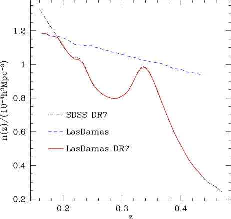
Data release 7 (DR7, Abazajian et al., 2009) is the last data release of the second phase of SDSS, know as SDSS-II. From the 929,555 galaxies, whose spectra have been measured, we use the subsample of luminous red galaxies (LRGs, Eisenstein et al., 2001) presented in (2010) and publicly available111http://cosmo.nyu.edu/~eak306/SDSS-LRG.html. The catalogue contains 89,791 LRGs, in the redshift range (), from the large contiguous area of in the Northern Galactic Cap. The full survey also includes three equatorial stripes, that we do not consider. This causes a loss of less than 10% in galaxy number and volume, but the resulting geometry is simpler. Furthermore, the use of the Northern Galactic Cap only allows us to obtain a more accurate estimate of the statistical errors than for the full survey (see Section 2.2). The dot-dashed line in Figure 1 shows a smooth spline fit to the sample number density as function of redshift. Together with the LRGs catalogue, we use a random one with about fifty times more objects, designed to reproduce the geometry and completeness of the galaxy sample and to have a radial number density proportional to the dot-dashed line in Figure 1.
| matter density | ||
| cosmological constant density | ||
| baryonic density | ||
| Hubble parameter [] | ||
| amplitude of density fluctuations | ||
| scalar spectral index | ||
| number of particles | ||
| box size [] | V | |
| particle mass [] | ||
| softening length [] |
2.2 The mock catalogues
In order to test our analysis technique and to estimate the covariance matrix associated to the LRG power spectrum, we use the LasDamas mock catalogues (McBride et al., in prep.). The mocks have been constructed from a suite of 40 large dark matter N-body simulations, dubbed Oriana, that reproduce a part of a universe characterised by a geometrically flat cosmology dominated by a cosmological constant and cold dark matter (CDM). The cosmological parameters and specifications of the simulations are listed in Table 1. From each simulation a halo catalogue is extracted using a Friend-of-Friend algorithm (FoF, Davis et al., 1985) with linking length 0.2 times the mean inter-particle separation. In order to match the LRG clustering signal, the haloes have then been populated with mock galaxies using a halo occupation distribution (HOD, , 2002) within the halo model approach (HM, see Cooray & Sheth, 2002, for a review). The HOD parameters have been chosen in order to reproduce the galaxy number density and the projected correlation function of the observed SDSS DR7 samples. From each simulation two (four) mock catalogues of the full SDSS DR7 volume (Northern Galactic Cap only) have been extracted. These mock catalogues, together with the mocks from two smaller companions of Oriana and the corresponding randoms, are publicly available 222 http://lss.phy.vanderbilt.edu/lasdamas.
In this work we use the 160 mock catalogues of the LRGs in the Northern Galactic Cap region. We modify the mocks and the corresponding random catalogue, which have the radial number density shown by the dashed line in Figure 1, in order to reproduce the one of the LRG: the resulting is indicated by the solid line. The mock catalogues contain on average 91137 galaxies.
3 The power spectra
From the dataset and the mock catalogues just described we compute the power spectra and the covariance matrix that are used in the rest of the analysis. They are presented in this section.
3.1 The LRG power spectrum
To compute the power spectrum and the window function we need to convert the angular positions and redshifts of the galaxies and of the random points into comoving coordinates. This is done first inferring radial distances from the measured redshifts and then converting the spherical coordinates into cartesian ones. To do the first step we assume as fiducial the cosmology of the LasDamas simulations, shown in Table 1.
We compute the power spectrum, as well as the survey window function, using the estimator introduced by (1994, thereafter FKP). (2004, thereafter PVP) proposed a modification of the FKP approach to take into account the relative biases between populations with different luminosities. In Appendix B.1 we show that, thanks to the fact that the LRG sample is almost volume limited and composed by a relatively homogeneous class of galaxies, the shape of the power spectra recovered with the two methods are in excellent agreement at linear and mildly non-linear scales. In Appendix A we summarise the most important equations of both estimators.
At first we correct the galaxy catalogue for the loss of objects due to fibre collisions (, 2002; Masjedi, 2006). The SDSS spectrographs are fed by optical fibres plugged on plates, which forces the fibres to be separated by at least 55”. It is then impossible, in a single exposure, to obtain spectra of galaxies nearer than this angular distance. The problem is partially alleviated by multiple exposures, but it is not possible to observe all the objects in crowded regions. Assuming that in a given region of the galaxies that satisfy the selection criteria we can measure only redshifts due to fibre collision and assuming that the missed galaxies have the same redshift distribution of the observed ones, we assign to the latter a weight . This ensures that the sum of the weights in a given region of the sky is equal to the number of selected galaxies . Secondly to each LRG and random object at position , where the number density is , we associate a weight , with . This value has been chosen in order to minimise the variance of the measured power spectrum in the range . In Appendix B.1 we show the results of the tests to analyse the impact of different choices of and corrections, namely fibre collision and completeness, on the recovered power spectrum.
To compute the power spectrum we assign the LRGs and the random objects, weighted as described before, to a cubic grid with cells and side using triangular shaped cloud (TSC) as mass assignment scheme (MAS). For each cell, we compute the field of equation (17a). We then perform the fast Fourier transform (FFT) using the publicly available software fftw333http://www.fftw.org/ (Fastest Fourier Transform in the West, Frigo & Johnson, 2005). We correct each Fourier mode by dividing it by , where is the Fourier transform of TSC, is the Nyquist wavenumber and is a 3D integer vector. Finally we spherically average the Fourier modes and subtract the shot noise (equation 21a).
The window function is evaluated similarly. We assign the objects of the random catalogue to four cubic grids with cells and sides and and compute the field of equation (22a). We use the four grids with different dimensions in order to be able to compute the window function up to very large scales. For each box, we perform the FFT, correct the Fourier modes, spherical average and subtract the shot noise (equation 23a). For each window function , we discard all the modes with wave-number and, when two or more window functions overlap, we consider only the one computed in the larger volume. This choice is motivated by the fact that, for a given band in wavenumber, the larger volume window function has been computed averaging over a larger number of modes than the ones from smaller volumes. Finally we merge the four window functions in order to obtain a single curve.
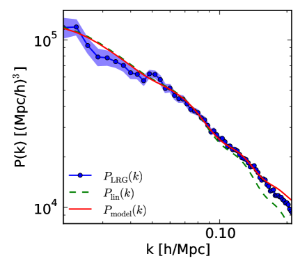
According to equation (20), the observed power spectrum just described is a convolution of the “true” power spectrum with the window function. This convolution is computationally time consuming, in particular when it has to be performed repetitively. Therefore we transform this convolution into a matrix multiplication:
| (1) |
is the window matrix normalised such that . The coefficients corresponding to the wavenumber are derived using the Gauss-Legendre decomposition. The second term in the right hand side arises from the integral constraint (Percival et al., 2007) where is a constant determined by requiring that .
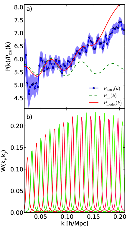
The LRG power spectrum is shown in Figure 2 with blue dots connected by a solid line. We also show the linear (green dashed line) and the model (red solid line) power spectra computed from the best fit parameters obtained assuming a flat CDM cosmology (see section 6.1 for more details). Both of the power spectra have been convolved with the window function as in equation (1) and their amplitude has been boosted in order to match the observed one. The blue shaded area represent the variance from the mock catalogues. Panel a) of Figure 3 shows the same quantities, with the same colour and line coding, but divided by a smooth linear power spectrum without BAOs (Eisenstein & Hu, 1998).
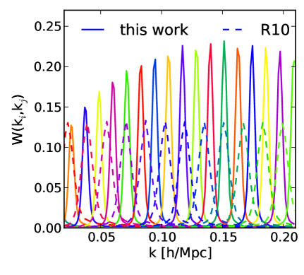
Panel b) of Figure 3 shows one every third row of the window matrix . Because of the relatively simple and uniform geometry of the sample used, the window function has its maximum at and decreases very steeply. This translates into the very sharp peaks at in the window matrix rows, as shown in the figure.
3.2 The mock power spectra and covariance matrix
We compute the power spectra from the 160 realisations and the window function as we do for the LRG sample in the previous section. We then compute the mean , the standard deviation and the covariance matrix C, whose elements are defined by:
| (2) |
where corresponds to the measurement of the power spectrum at the -th -bin in the -th realisation.
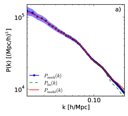
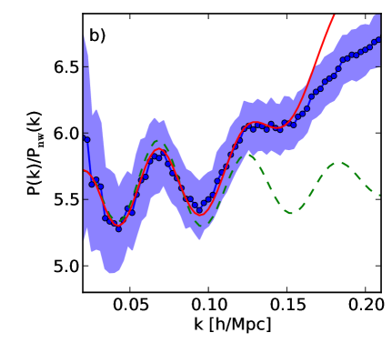
Panel a) of Figure 4 shows the mean power spectrum and its variance (blue dots with solid line and shaded area) obtained from the mock catalogues. The green dashed and the red solid lines show the linear and the best fit model power spectra (see Section 5.4.1 for more details) convolved with the window function of the mocks and rescaled by the bias. Panel b) of Figure 4 shows the same power spectra of panel a) divided by a power spectrum without oscillations .
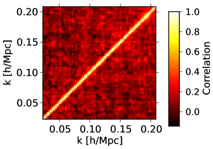
The correlation matrix of the mock catalogues, defined as , is shown in Figure 5. The mode correlation caused by the convolution with the window function is visible in particular near the diagonal. Non linear mode coupling is present at small scales and its strength increases with increasing . Although the correlation becomes important for , it is not negligible already at . Recently (2011) showed that different methods of constructing the random catalogues can affect the estimated covariance matrix.
The version of the mocks available when writing this article does not contain information about the luminosity of the galaxies, completeness and fibre collision. We cannot therefore test the impact of different estimators and corrections on the errors. However we analyse the impact of different on the power spectra and errors as measured from the mocks: the results are reported in Appendix B.2.
4 Additional experiments
Later in this article we use the measurement of the LRG power spectrum described in the previous section to constrain cosmological parameters. In order to obtain tight constraints it is not possible to use this measurements alone, since some parameters have a weak dependence on the shape of the power spectrum and others present strong degeneracies. Using the information coming from independent experiments, like the cosmic microwave background (Section 4.1) and the type 1a supernovae (Section 4.2), or prior knowledge of some of the parameters, like the local Hubble parameter (Section 4.3), it is possible to greatly improve the accuracy of the analysis.
4.1 Cosmic microwave background
Accurate measurements of the CMB temperature and polarisation anisotropies provide a powerful tool to constrain cosmological parameters. In this work we use the observations from five different instruments.
The Wilkinson Microwave Anisotropy Probe (WMAP) satellite produced full sky maps of the CMB with a resolution of . We make use of the temperature angular power spectrum in the multipole range and the temperature-E polarisation cross power spectrum in the range from the 7th year data release (WMAP7, , 2010, 2011, 2011).
We also use measurements of higher multipoles from other four experiments which observe the CMB temperature anisotropy on small patches of the sky with a much higher resolution. In order to avoid complex correlations, we use these experiments only for multipoles that do not overlap with the WMAP measurements. We use the measurements of the temperature angular power spectrum i) in 14 bandpowers in the range from the Arcminute Cosmology Bolometer Array (ACBAR, , 2007, 2009), ii) in 6 bandpowers in the range from the Cosmic Background Imager (CBI, for latest results see , 2009), iii) in 7 bandpowers in the range from the 2003 flight of the Balloon Observations Of Millimetric Extragalactic Radiation and Geophysics (BOOMERanG , 2006, 2006, 2006, 2006) and iv) in 11 bandpowers in the range from the final data release of QUEST at DASI (QUAD, for latest results see , 2009) . We also use E and B polarisation (EE and BB) and the cross temperature-E polarisation (TE) angular power spectra measurements from the latter three experiment. i) CBI: EE in 7 bandpowers in the range , BB in 5 bandpowers in the range and TE in 8 bandpowers in the range ; ii) BOOMERanG: EE and BB in 3 bandpowers in the range and TE in 6 bandpowers in the range ; iii) QUAD: EE, BB and TE in 17 bandpowers in the range .
4.2 Type 1a supernovae
Type 1a supernovae (SNIa) provided the first evidences of an accelerating Universe and the need of a new exotic component, called dark energy, to explain it (Riess et al., 1998; Perlmutter et al., 1999). From the light curve, i.e. the luminosity variation as function of time, of a SNIa it is possible to measure the absolute luminosity, from which the distance to each object is inferred, probing in this way the distance-redshift relation. The first step is performed thanks to models which encode intrinsic variations due to the physics of the SNIa, the effects from galactic and intergalactic medium and selection effects in different ways. Because of this, models produce different results, which impact the accuracy at which cosmological parameters can be measured and can introduce systematic effects (e.g. , 2009, 2009).
SNIa data have been collected by many surveys designed according to different strategies and carried out using a large variety of telescopes. Each of them observes a relatively small number of events, typically less than a hundred. In order to increase the number of objects, recently collections of SNIa from different surveys have been created. In this work we use one of such samples, the Union2 (, 2010). It consists of 557 SN drawn from 17 datasets in the redshift range and is the largest available supernovae sample to date. It extends and improves the Union (Kowalski et al., 2008) and the Constitution (, 2009) datasets: all the light curves of the selected SNIa have been fitted with salt2 (, 2007) and an improved analysis of systematics is presented. (2010) showed that the inclusion of systematic errors when fitting cosmological parameters, using only SNIa or in combination with independent probes (BAO, CMB and ), increases the associated errors leaving the best fit value almost unchanged. In Sections 6.1 and 6.3 we will further comment on the impact of systematics and of light curve fitters.
4.3 Hubble parameter
The Supernovae and H0 for the Equation of State Program (SHOES, , 2009) aims at the direct measurement of the Hubble parameter at present epoch to better than accuracy. The SHOES team identified 6 nearby spectroscopically typical SNIa, that have been observed before maximum luminosity, that reside in galaxies containing Cepheids and that are subjects to low reddening. Thanks to 260 Cepheids observed with the Near-Infrared Camera and Multi-Object Spectrometer (NICMOS) on the Hubble Space Telescope (HST) in the 6 host galaxies and in the “maser galaxy” NGC 4258, the authors could calibrate directly the peak luminosity of the SNIa. Combining these 6 objects with 240 SNIa at redshift , they measure the Hubble parameter to be . The error includes both statistical and systematic uncertainties. In this work we use this result as a prior knowledge of H0, under the assumption that the associated likelihood is a gaussian with the mean and standard deviation measured by the SHOES team.
5 Methodology
In this section we describe the model for the full shape of the power spectrum that we use throughout the rest of this article (Section 5.1). In Sections 5.2 and 5.3, we present the parameter spaces explored in Section 6 and the method used to extract cosmological information. Finally, we test the model against the LasDamas and the LRG power spectra (Section 5.4).
5.1 The model
M10 introduced a model for the full shape of the power spectrum inspired by renormalized perturbation theory (RPT, Crocce & Scoccimarro, 2006a, b) and analogous to the one for the correlation function of Crocce & Scoccimarro (2008) and Sánchez, Baugh & Angulo (2008). In this model they parametrize the non-linear power spectrum as
| (3) |
where the linear bias , the damping scale of the BAO oscillations and amplitude of the mode coupling contribution are free parameters. is the linear power spectrum and
| (4) |
is the lowest order term arising from the coupling of two initial modes. The exponential damping and are the approximations of the non-linear propagator and of the mode coupling power spectrum described by RPT.
The model of equation (3) has been successfully tested in M10 against a suite of very large, median resolution N-body numerical simulations, called L-BASICC II (Angulo et al., 2008; Sánchez, Baugh & Angulo, 2008). M10 computed power spectra for the dark matter distribution and several halo samples, selected according to their mass, both in real and redshift space at z=0, 0.5 and 1. They have shown that in all cases equation (3) describes accurately these power spectra for and that it allows to obtain unbiased constraints on cosmological parameters.
5.2 Parameter spaces
In the description of the datasets presented in Sections 2-4, a strong assumption was implicitly made: the Universe is, at large scales, statistically homogeneous and isotropic and that density and velocity fluctuations around their mean values are small. In the following, we further assume that the fluctuations set by the initial conditions were adiabatic, gaussian and almost scale invariant and that they do not present tensor modes. The WMAP7 data, both alone and in combination with BAO, and SNIa, confirm that those assumptions are correct at the confidence level (, 2011, 2011).
Within this framework we analyse five different cosmological models, explored using five combinations of experiments: CMB, CMB+, CMB++, CMB++SNIa and CMB+++SNIa.
The “concordance” CDM model is the simplest model able to successfully describe a large variety of cosmological datasets. It describes a geometrically flat () universe with a cosmological constant , whose equation of state parameter is constant in space and time, and pressureless cold dark matter (CDM) as main components. This cosmology can be characterised by six parameters: the baryon and dark matter densityies and , the scalar spectral index and the amplitude of the primordial fluctuations, the optical dept to the last scattering surface, assuming instantaneous reionisation, and the ratio between the horizon scale at decoupling and the angular diameter distance to the corresponding redshift :
| (5) |
The four parameters after the semicolon are related to the modelling of the matter power spectrum ( and from equation 3) and of the CMB angular power spectrum (, amplitude of the contribution to the CMB at large from the Sunyaev-Zeldovich effect). These parameters are marginalised over when showing the cosmological constraints in the section 6.
If we then drop one or both assumptions on geometry and on the value of the dark energy equation of state, we obtain three cosmologies characterised by the following parameter spaces:
-
•
variable curvature, :
(6) -
•
zero curvature, :
(7) -
•
variable curvature, :
(8)
As last case, we consider a flat Universe in which evolves with time. We adopt the parametrisation proposed by (2001) and (2003):
| (9) |
Although not physically motivated, it can describe accurately a big variety of equations of state derived from scalar fields with the use of only two parameters: its value today, , and its first derivative with respect to , . The resulting parameter space is:
| (10) |
Other cosmological quantities can be derived from the ones just listed. In particular we are interested in:
| (11) |
The density of dark energy, , is obtained from a combination of , and . From there, the total matter density , the Hubble parameter and the age of the universe are derived. The present day of linear density fluctuation in a sphere of radius , , is computed from . From , , and it is possible to estimate the redshift of reionisation (, 1994).
5.3 Practical issues
| Parameter | lower limit | upper limit |
| 0.005 | 0.1 | |
| 0.01 | 0.99 | |
| -0.3 | 0.3 | |
| () | -2 | 0 |
| -2 | 2 | |
| 0.5 | 1.5 | |
| 2.7 | 4 | |
| 0.01 | 0.8 | |
| 100 | 0.5 | 10 |
| 0.01 | 0.35 | |
| 0 | 5 | |
| 0 | 2 |
To constrain the sets of cosmological and model parameters just described, we use the Markov Chain Monte Carlo technique (MCMC, Gilks, Richardson & Spiegelhalter, 1996; Christensen & Meyer, 2000) as implemented in the free software cosmomc444http://cosmologist.info/cosmomc/ (Cosmological MonteCarlo, Lewis & Bridle, 2002). The CMB and linear matter power spectra are computed with a modified version of camb (Code for Anisotropies in the Microwave Background, , 2000) that allows to consider time varying 555http://camb.info/ppf/(Fang, Hu & Lewis, 2008). For each choice of parameter space and probes we run eight independent chains. Their execution is stopped when the Gelman & Rubin (1992) criterion is satisfied. The MCMC requires some prior knowledge of the parameter space that is explored. We assume for all the primary parameters (equations 5-8 and 10) flat priors in the ranges listed in Table 2. The model parameter is analytically marginalised over an infinite flat prior (equation F2 in Lewis & Bridle, 2002).
All likelihoods used to compare the results from the cosmological probes described in sections 2.1, 4.1, 4.2 and 4.3 with the corresponding models are assumed to be Gaussian. In the case of the LRGs power spectrum, this is
| (12) |
where
| (13) |
is the standard , in which is an array containing the band power , contains the model computed for the set of parameters and then convolved with the window function and C is the covariance matrix of the measurement presented in section 3.2.
In section 2.1 we assume a fiducial cosmology in order to convert redshifts and angles to physical coordinates. Different choices of these parameters result in modifications of the measured LRG power spectrum. The ideal case would be to recompute, for each step of the MCMC chain, the power spectrum and the window function according to the given cosmology, but this is not computationally feasible. Under the assumption that the survey covers a wide solid angle, it is possible to incorporate these distortions in the correlation function when computed using different cosmologies by rescaling the distance scale by the factor (, 2005):
| (14) |
where the effective distance to the mean redshift of the sample is,
| (15) |
with the comoving angular diameter distance. Since the power spectrum is the Fourier transform of the correlation function, this holds also for the former. Thus, at each step of the chain we multiply the wave-number of the model power by and its amplitude by in order to rescale it to the fiducial cosmology.
5.4 Testing the model
In the first part of this section we extend the analysis of M10 and fit our model against the mock catalogues in order to test wether it provides an accurate description of the measured power spectrum and unbiased constraints of the dark energy equation of state parameter also when a complex geometry is involved. We also test the stability of the cosmological parameters in the wCDM case as the maximum included in the analysis varies, when CMB and the are combined.
5.4.1 Mock catalogues
In this section we follow M10 and assume all the parameters fixed, except for . Under this assumption, equation (14) links univocally variations of the dark energy equation of states to stretches of the model power spectrum. Therefore we consider the latter as a a free parameter (Huff et al., 2007).
Using a MCMC approach, we explore the parameter space defined by . We chose priors with a constant probability within the following ranges:
-
•
,
-
•
,
-
•
.
The bias is marginalised analytically over an infinite flat prior as described in section 5.3.
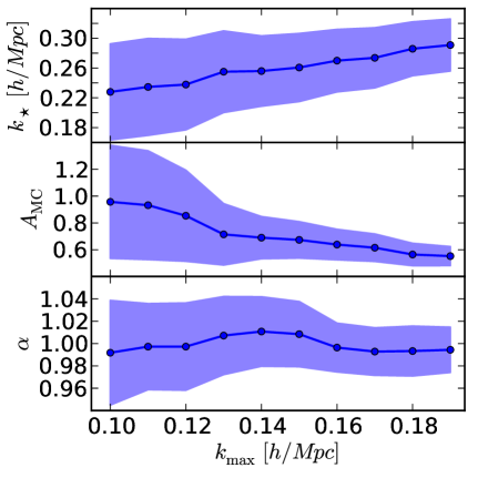
Figure 6 shows the one-dimensional marginalised constraints on the parameters , and varying the maximum value of the wave number of the measured power spectrum used to perform the fit; we keep the minimum fixed to . The blue circles connected by solid lines and the shaded areas correspond to the mean and the standard deviation of these parameters. For every the model is evaluated for and then convolved with the window function. Since each row of is sharply peaked at , the main contribution to comes from modes near : therefore the constraints shown in Figure 6 depend weakly on the exact wave number range in which the model is computed, as long as it is larger than the range of the measured power spectrum that we fit. As increases, more modes are included in the fit and the errors decrease. The constraints on are compatible with unity for all the considered. Considering that the volume of the simulations used in M10 is much larger that the one sampled by the LRGs and consequently that the errors in the former case are smaller than in the latter, we decide to further consider scales . The constraints on and exhibit, respectively, a monotonic increase and decrease. As explained in M10, the approximate mode coupling power in equation (3) is about larger than the exact value at : this forces to decrease to and to increase in order to maintain the shape of the resulting power spectrum unvaried.
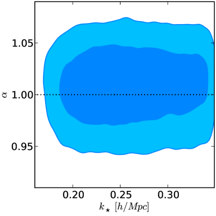
Figure 7 shows the two-dimensional marginalised constraints in the plane as obtained from the mock catalogues for . The inner dark and outer light shaded areas represent regions whose volumes are and of the total likelihood. This representation of the two-dimensional constraints will be used through all section 6. The independence of from or makes the constraints on the former robust. The latter two parameters, instead, are strongly degenerate, as it is possible to describe accurately the overall shape of the power spectrum compensating an increase (decrease) of with a decrease (increase) of .
5.4.2 The Luminous red galaxy sample
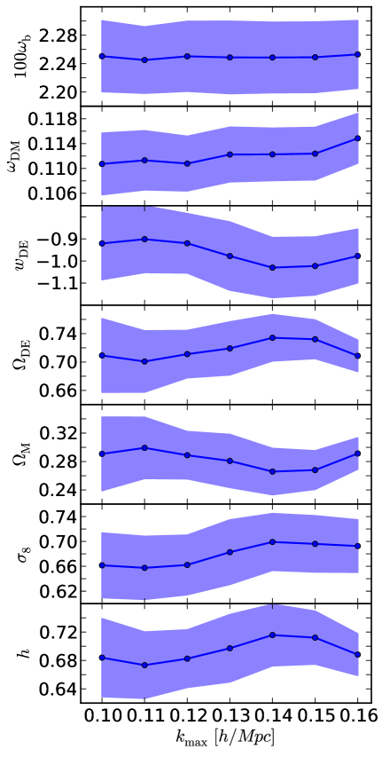
After testing the robustness of our model at mildly non-linear scales, we test here the dependence of the cosmological parameters upon . We use the wCDM cosmology defined in equation (7) and the combination of the LRG power spectrum and CMB measurements. Figure 8 shows the one-dimensional marginalised constraints on the parameters , , , , , and as function of . The circles connected by solid lines and the shaded areas show the mean and the standard deviation as obtained from the MCMC. The model is computed for and then convolved with the window function; as before, the measured parameters are mostly insensitive to this limit. Although some parameters are more stable with respect to changes of than others, there are no significant trends or deviations. The error-bars of the parameters decrease as increases: we interpret this as a sign of new information coming from these scales.
We also test the impact of using CMB measurements from WMAP only. We obtain the same constraints, but with errors larger by 5-10%, due to the loss of information at small angular scales, i.e. large multipoles . Appendix B.3 describes how the results just described depend upon and . A more extensive analysis of the wCDM cosmology is presented in section 6.3.
6 Results: the cosmological parameters
In this section we present the constraints on the cosmological parameters obtained from the five cosmological scenarios introduced in section 5.2.
6.1 The concordance cosmology
| CMB | CMB+ | CMB++ | CMB++SNIa | CMB+++SNIa | |
|---|---|---|---|---|---|
| 100 | |||||
The flat CDM cosmology, parametrized by the first six quantities of equation (5), is the minimal model able to describe data coming from many independent probes. Table 3 summarises the complete list of one-dimensional constraints for the primary and derived cosmological parameters obtained in this section. We quote the mean values and width of the posterior distribution containing 68% of the total area, which for a Gaussian distribution corresponds to the standard deviation, as obtained for the five different combinations of the four experiments used in this work. This convention will be followed in the rest of this article.
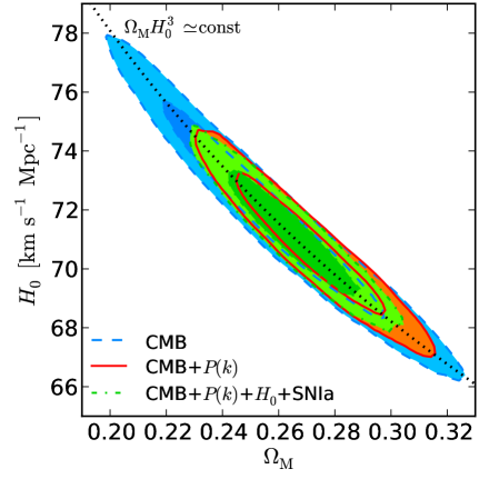
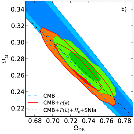
The CMB experiments described in section 4.1 provide measurements of the temperature and polarization angular power spectra with very high accuracy. The blue shaded areas enclosed in dashed lines in Figure 9 show the 68% and 95% confidence level in the as obtained when CMB information only is used. The apparent position of the peaks in the CMB power spectra is proportional to their physical scale, which depends on the composition of the early universe (baryons, dark matter and radiation), and the angular diameter distance to the last scattering surface, a function of and of the density and equation of state parameter of matter, dark energy and of curvature. Since here we consider a flat geometry and fix to -1, a degeneracy between the matter density and the Hubble parameter appears. It has been shown by Percival et al. (2002) that this effect, together with the preservation of the relative amplitude of the peaks, leads, in a CDM universe, to a degeneracy along the curve defined by , which is displayed in Figure 9 by the dotted line. The accurate detection of the third peak in the temperature power spectrum, whose relative amplitude with respect to the first two is proportional to the matter-radiation ratio, helps reducing this degeneracy. In this case we measure , and .
The inclusion of information from the large scale structure can break or reduce some of the degeneracies in the CMB. The shape of the power spectrum depends upon and, more weakly, (e.g., Efstathiou et al., 2002; Sánchez & Cole, 2008). Thanks to this, the errors on the cosmological parameters decrease up to about 30%. In particular, we measure a decrease in the allowed region by about one third in the three parameters considered before: , and . The two-dimensional constraints in the plane are shown in Figure 9 with the red shaded areas within solid lines.
When the SNIa and H0 measurements are also used, we obtain , and , which means a 10-15% increase in accuracy. The two dimensional 68% and 95% confidence levels for the former two parameters, when all the four probes are used, are shown in Figure 9 by the green shaded areas enclosed by dot-dashed lines.
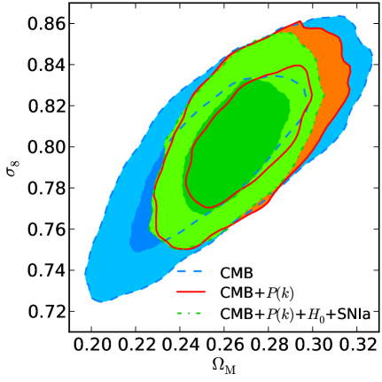
Figure 10 shows the two-dimensional marginalised constraints in the plane for the same combination of datasets; colour and line coding is the same as in Figure 9. The correlation between the two parameters is caused by the fact that an increase (decrease) of causes a decrease (increase) in the amplitude of the power spectrum that can be compensated by a larger (smaller) value of . For the three cases shown in the figure we find that the one-dimensional constraints on the latter parameter are, respectively, , and ; the error on the latter two decreases by 20 and 22% respectively to the CMB only result.
The solid lines in Figures 2 and 3 show the model power spectrum computed using the cosmological parameters listed in the last column of Table 3 and the best fit model parameters and , as obtained from the MCMC for . The bias has been computed maximising the likelihood of equation (12) with all the other parameters fixed.
| no systematics | mlcs2k2 | |
|---|---|---|
| 100 | ||
Effects of supernovae systematics and light curve fitters
| CMB | CMB+ | CMB++ | CMB++SNIa | CMB+++SNIa | |
|---|---|---|---|---|---|
| 100 | |||||
Uncertainties in the modelling of SNIa can affect the cosmological parameters and associated errors extracted using a given dataset. To test the impact of systematics and light curve fitters on the results just presented, we re-analyse the CDM cosmology with two different SNIa settings. First we use the same Union2 set, but neglecting the systematic errors provided with the data; second we substitute this dataset with the Sloan Digital Sky Survey-II Supernova Survey sample (SDSS SN, , 2009). The sample consists of 288 supernovae from 5 different experiments whose light curves have been fitted both with the mlcs2k2 (, 2007) and salt2 models. Since most of the objects in SDSS SN are also part of the Union2, we do not expect large differences between the two samples if salt2 is used. Therefore we show here only the results obtained using the mlcs2k2 fitter. The one-dimensional constraints that we extract from the combination of all four probes, when the systematics in the Union2 are ignored and when the SDSS SN with mlcs2k2 are used, are listed in Table 4. As expected, and in agreement with (2010), ignoring systematic errors globally reduces the errors on the recovered values of the parameters without changing sensibly the mean value. As example we obtain (14% decrease with respect to the corresponding case in Table 3), (12%), (14%) and (5%). On the other hand, the use of mlcs2k2 changes the posterior distribution sensibly, without influencing its width. We measure that , and change by more than 1.5-2. This shift agrees with the findings in (2009) and (2011) and suggests, in our opinion, that the choice of the model used to fit the light curves can bias sensibly the cosmological results obtained.
6.2 Curvature
In this section we analyse the cosmological constraints obtained when the curvature is considered as a free parameter. The full list of parameters (mean plus the 68% confidence level) is shown in Table 5 for the combination of experiments listed in the header of the table.
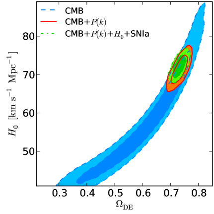
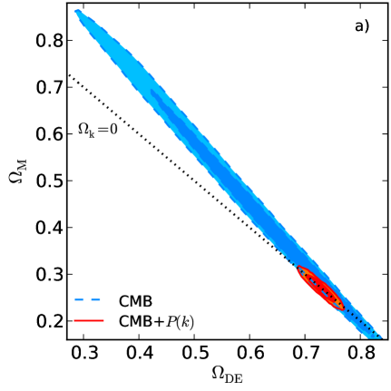
The blue shaded areas within dashed lines in panel a) of Figure 11 and in Figure 12 show the two-dimensional marginalised constraints in the and planes, respectively, as obtained from CMB data alone. The plots show a very strong degeneracy between these parameters. As stated in Section 6.1, the apparent size of the CMB acoustic peaks depends on their physical size and the angular diameter distance. Given that curvature density is small and that it scales as the inverse square of the scale factor, it affects much more than the dynamics of the early universe. It is always possible to find combinations of , and that keeps the angular size of the CMB peaks constant. Therefore, the constraints on the derived parameters are much weaker than the ones obtained in the previous section: , and . The measured curvature, , is compatible with flatness at about the 1 level.
Both panels in Figure 11 and Figure 12 show, with red shaded areas enclosed in solid lines, the same parameter planes as above when explored combining CMB and large scale structure information. Panel b) of Figure 11 shows a zoom of the constraints of panel a) in the area around and in order to show with more details the constraints obtained when more information is added to the CMB data. The galaxy power spectrum is very sensitive to the matter density. Additionally the BAOs allow to measure the angular diameter distance to the mean redshift of the LRG sample, . The degeneracies in the CMB alone are therefore strongly reduced when LSS measurements are included. The four variables discussed in the previous paragraphs become , , and : their errors are almost one order of magnitude smaller than in the CMB only case. With respect to the corresponding CDM case, the uncertainties on the first three quantities increase up to 50%.
The inclusion of SNIa and measurement, decreases the errors on curvature by about 10% () and on the other three parameters considered before by circa 20% (, and ). When comparing with the results from the previous section, the errors on dark energy and matter density are unchanged, while increasing by less than 40% for the Hubble parameters. The two-dimensional marginalised constraints in the and planes are shown in panel b) of Figure 11 and in Figure 12 with green shaded lines enclosed in dot-dashed lines.
6.3 Beyond the cosmological constant
| CMB | CMB+ | CMB++ | CMB++SNIa | CMB+++SNIa | |
|---|---|---|---|---|---|
| 100 | |||||
In sections 6.1 and 6.2 we assume that dark energy is modelled as a cosmological constant. Despite its simplicity and its success in describing simultaneously many independent observations, the present day value of the density of dark energy does not have a solid physical explanation; this led, in the past decade, to the exploration of a large number of alternative model, most of which present a time dependent equation of state666All theories of modified gravity can be also represented through an effective .. Ideally, one would like to be able to constrain the full time, or redshift, dependence of in order to restrict the range of possible models. Usually, parametric forms for the dark energy equation of state are assumed, which allow to measure time dependencies, but do not necessarily reproduce the correct . With non-parametric approaches and principal component analysis it is possible to overcome some of these limitations (e.g., , 2003, 2009, 2010). In this section we assume the simplest parametric form possible: is a constant, independent of time, with a flat prior in the range . Deviations from the value would suggest that the cosmological constant is not a viable model of dark energy. If this is the case, the results shown in the previous two sections could be biased as consequence of wrongly assuming that dark energy is described by . In section 6.5 we analyse an alternative scenario in which is parametrized as a linear function of the scale factor.
Table 6 lists the constraints on the cosmological parameters as obtained for the different combinations of datasets analysed in this work. They are in perfect agreement with the ones presented with the previous two parameter spaces.
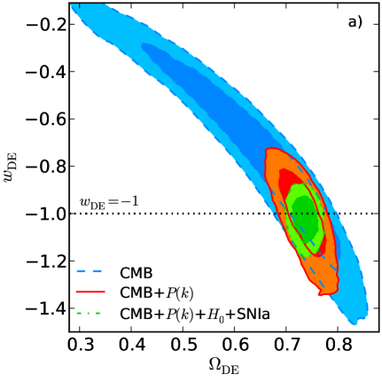
Panel a) of Figure 13 shows the constraints in the plane. The horizontal dotted line corresponds to . If the CMB alone is considered a strong degeneracy between these two parameters is present, as shown by blue shaded areas enclosed by dashed lines. The reason for this degeneracy is analogous to the case analysed in the previous section when curvature is left as free parameter. In fact, while dark energy is subdominant at early times and does not influence the physical scale of the acoustic peaks, its equation of state parameter and density have a strong effect on the angular diameter distance to the last scattering surface. Thus different combinations of , and can result in the same apparent position of the acoustic oscillations in the CMB temperature power spectrum. The constraints on the dark energy density and equation of state parameter are therefore very weak: and .
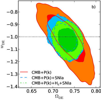
With the inclusion of the LRGs data, the degeneracies in the CMB are broken, as shown in the panel a) of Figure 13 (solid line enclosing red areas). From the same figure it is clear that the impact of supernovae and (dot-dashed line enclosing green areas) information is much larger in this scenario than in the previous two. In order to understand what causes such a difference, we show in panel b) of Figure 13 also the two dimensional constraints obtained from the combination of CMB++SNIa (dashed lines enclosing blue areas). The horizontal line corresponds to . The plot shows clearly that supernovae have a large constraining power for this parameter space. In fact the supernovae luminosity-distance relation traces the expansion history of the Universe and clearly identifies the transition between the deceleration and acceleration phases (, 2004). This transition depends on the densities of the cosmic components and is very sensitive to the dark energy equation of state. The inclusion of a precise measurement of increases the precision on the parameters by a small factor. The constraints on the dark energy equation of state are i) , from CMB+, ii) , from CMB++, iii) , CMB++SNIa and iv) , from CMB+++SNIa. Therefore the inclusion of the large scale structure measurements decreases the error on by about a factor 3 and SNIa further halve it.
The main result of this section is that, when combining CMB, LSS, SNIa information with the prior on , the equation of state parameter of dark energy is constrained to be -1 with about 6.5% accuracy. This, although perfectly compatible with the cosmological constant models, does not exclude other dark energy scenarios. Excluding CMB, which has very little constraining power, the other three experiments give us access only to redshift . Furthermore many dark energy models can be tuned in order to mimic at low redshifts and deviate from it at earlier epochs. In order to narrow the range of possible models, more precise measurements spanning a larger range of redshifts, together with the inclusion of tests of the growth of structures, will be necessary.
Effects of supernovae systematics and light curve fitters
| no systematics | mlcs2k2 | |
|---|---|---|
| 100 | ||
Similarly to what has been done in section 6.1, we test the impact of SNIa systematic effects and different light curve fitters on the measured cosmological parameters. The constraints for these two cases are listed in Table 7. As before, we find that neglecting systematics does not change the mean values of the parameters, but generally reduces the associated errors. In particular the constraints on the dark energy equation of state are reduced by almost 30%, . The use of the data from the SDSS SN project, with the light curves fitted with mlcs2k2, changes some of the parameters, as for instance , and , by more than 2- with respect to the value in our standard case. In particular we measure to be . This highlights, better than for the CDM case, the importance of SNIa modelling in improving cosmological constraints from future generation experiments.
6.4 Curvature and dark energy equation of state as free parameters
| CMB | CMB+ | CMB++ | CMB++SNIa | CMB+++SNIa | |
|---|---|---|---|---|---|
| 100 | |||||
We now analyse the accuracy that can be achieved when both and are considered as free parameters. The full list of constraints on the cosmological parameters for the kwCDM cosmology is summarised in Table 8.
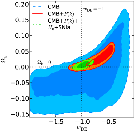
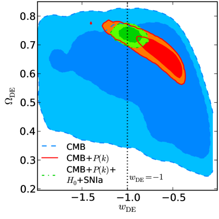
The introduction of an extra degree of freedom with respect to the previous two sections affects the CMB degeneracy already discussed. The two-dimensional marginalised constraints in the and planes from CMB data only are shown in Figures 14 and 15 with the blue shaded areas within dashed lines. By comparing Figure 15 with panel a) of Figure 13 it becomes clear that the allowed area in the parameter space increases because of the larger degeneracy. This causes the errors on and to increase by 50-60% with respect to the corresponding cases in sections 6.2 and 6.3.
The red contours within solid lines in Figures 14 and 15 show the constraints in the and planes from the combination of CMB with the LRG data. The inclusion of the power spectrum reduces the region allowed by CMB alone to a one-dimensional degeneracy, that can be broken using the information on the amplitude of . Therefore a degeneracy arises between the bias and the shape of the power spectrum when both the curvature and the dark energy equation of state are treated as free parameters. When considering the range of scales larger values of , and and lower values of can be compensated by unphysically large biases and larger values of in order to obtain a comparable . If we used a finite flat prior on we would decrease the large and tail and reduce the degeneracy. Alternatively, the detection of the turnover in the power spectrum, not possible nowadays because of the still too small volumes probed by galaxy surveys, might help constraining better its overall shape and break the degeneracy just described.
The addition of and supernovae measurements breaks the bias-shape degeneracy, returning parameters perfectly consistent with the CDM cosmology. As for the previous section, the biggest change in precision is due to the SN, which improves the accuracy of the three parameters previously discussed, by a factor 2-3. The final constraints, when all four probes are used, are shown in Figures 14 and 15 by the green shaded areas enclosed within dot-dashed lines. For the quantities shown in the plot we obtain (36% increase in the errors with respect to kCDM case), (29% increase in the errors with respect to the wCDM case) and (8% increase with respect to both).
6.5 Time varying dark energy equation of state parameter
| CMB | CMB+ | CMB++ | CMB++SNIa | CMB+++SNIa | |
|---|---|---|---|---|---|
| 100 | |||||
In section 6.3 we encode possible deviations from the cosmological constant model in a constant effective dark energy equation of state. In this section we include explicitly a time dependency on through the simple parameterization of equation (9). We treat the two parameters of this model, and as free and we consider the curvature to be fixed 0. The constraints on the cosmological parameters for the cosmology analysed in this section from the different combinations of probes are listed in Table 9.
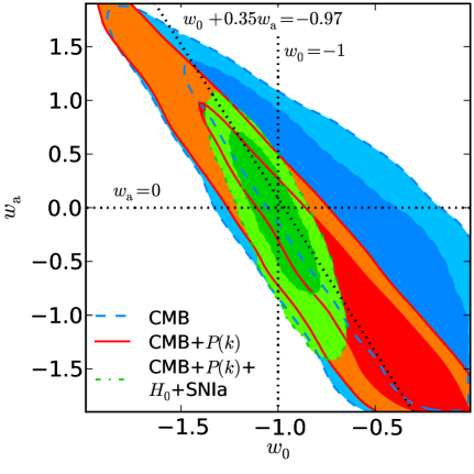
Figure 16 shows the two-dimensional marginalised constraints in the plane from CMB alone (blue shaded areas within dashed lines), CMB plus LRG power spectrum (red shaded areas within solid lines) and the combination of CMB, , and SNIa (green shaded areas within dot-dashed lines). The vertical and horizontal dotted lines at and show the values of the two parameters for the CDM case. In the three cases a degeneracy is visible, which is reduced as more independent data are included. From CMB alone we obtain and ; the inclusion of the LRGs power spectrum information does not change substantially the one-dimensional constraints ( and ) but reduces by almost a factor 2 the figure of merit, i.e. the area of the 95% confidence level (, 2006). As shown in the previous two sections, supernovae have an important role in constraining dark energy properties and the inclusion of their infomation reduces the errors in the two parameters by about a factor 3 and 2, respectively. The one-dimensional constraints from the combination of all the datasets are and . The attempt to constrain also the time evolution of the dark energy equation of state results in a degradation of its present value.
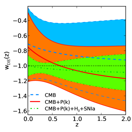
From these results it is possible to reconstruct the time dependence of the dark energy equation of state parameter. The thick dashed, solid and dot-dashed lines in Figure 17 show the value of from CMB, CMB plus and the combination of the four probes, respectively. The corresponding 1- errors, which vary with redshift, are indicated by the shaded areas within the thin lines. They are computed according to (2006):
| (16) |
In the redshift range shown in the plot, is always compatible with a cosmological constant at the 1 level. Furthermore the errors show a minimum at a redshift called “pivot” (, 2001, 2004, 2006). For the three cases shown in Figure 17, we obtain a pivot redshift of (CMB), (CMB+ and (CMB+++SNIa) and an equation of state parameter , and . It is interesting to note that in the last case the precision is comparable to the one presented in Section 6.3. The diagonal dotted line in Figure 16 shows that the degeneracy between and is very close to , where is the pivot scale factor from the CMB+ constraints.
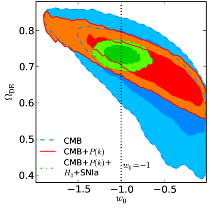
Figure 18 shows the two-dimensional marginalised constraints in the plane. The colour and line code is the same as in Figure 16. This figure illustrates that the addition of large scale structure information to the CMB data halves the errors on the dark energy density from to . The inclusion of SNIa and H0 measurements decreases the errors further by 70% to .
7 Comparison with previous studies
In this section we compare our results with recent work focused on the analysis of the large scale structure of the Universe. In Section 7.1 we perform a quantitative comparison of our results with those of Reid et al. (2010, thereafter R10), whose measurement and model are publicly available777http://lambda.gsfc.nasa.gov/toolbox/lrgdr/. Section 7.2, instead, lists a number of similar analyses, for which this is not the case, and we can only discuss the differences qualitatively.
7.1 Reid et al. (2010)
The LRG distribution from the SDSS DR7 has already been used to extract cosmological parameters by R10. The analysis in that work differs from the one we perform mostly in five important details: i) all the LRGs from the Northern Galactic Cap and the 3 southern stripes were used (110576 galaxies in 7931 deg2), ii) thanks to the count-in-cylinders technique (CiC, Reid & Spergel, 2009; Reid et al., 2009), the authors extracted a halo catalogue from the LRG distribution and then computed the halo power spectrum using the PVP estimator, iii) they computed the covariance matrix from 10000 lognormal catalogues (LN, , 1991), iv) they used a model based on halofit (, 2003), that required additional calibration against numerical simulations and v) they analysed the power spectrum in the range . The advantage of using the reconstructed underlying density field, instead of the galaxies, is that the intra-halo peculiar motions, which cause the so called fingers-of-gods, are erased, leaving weaker small scale redshift-space distortions. They combine their halo power spectrum with the 5th year data from the WMAP satellite (WMAP5, Komatsu et al., 2009) and the Union Supernovae dataset (Kowalski et al., 2008). The comparison between the results in table 3 of R10 and the corresponding ones in this work (third column in Tables 3, 5, 6 and third and fifth columns in Table 8) shows that, with the exception of the CDM case and despite the smaller modes used by us, the errors that we obtain here are slightly smaller and that there are significant offsets in the preferred values of some parameters. For example, the constraints on in the wCDM parameter space, when combining CMB and , are in our analysis and in R10.
| this work | vs. | vs. | vs. | vs. | |
|---|---|---|---|---|---|
| R10 model | our model | R10 model | R10 model, extended | ||
| 100 | |||||
As the full measurement from R10 and a cosmomc module which includes the model is publicly available, we can understand the origin of the differences between the two studies. We concentrate here on the wCDM parameter space. Table 10 compares the results shown in the third column of Table 6 (second column) with the constraints that we obtain applying i) R10 model to our measurement (third column), ii) our model to R10 measurement (fourth column) and iii) R10 model to R10 measurement (last two columns). To do it, we combine the large scale structure information with the CMB measurements presented in Section 4.1, we consider the scales and we compute the model for before the convolution with the window function. In the last column we use and , as originally done in R10. The similarity between the constraints obtained in this last case and those of R10 shows that the effect of using WMAP7 plus small angular scale CMB data instead of WMAP5 is very small. If we consider the parameters constrained mainly by the CMB (, , , , , and ) we find that they are, as expected, mostly independent of the power spectrum measurement and model used in the analysis. Excluding the last column, for the other parameters we find i) that, given a measurement, the errors that are obtained using the model of equation (3) are generally smaller than the ones from R10’s model and ii) that, given a model, the parameters obtained from our measurement agree better with the bulk of the literature than the ones recovered from the R10 power spectrum. In particular, these data prefer larger values of and of , which lead to smaller values of and . Using presented in Section 3.1 we measure the dark energy equation of state parameter to be when using our model and when using R10 model. This is more than a 50% increase in the uncertainty. If we consider the R10 measurement, we obtain, for the two models, and , with at 1.5 and 0.9 level, respectively. Including scales up to , we measure : the error decreases, but remains larger than when using our model, and disfavours the cosmological constant scenario at 1.2. These results clearly point towards differences in both the modelling and the measurement of the power spectrum.
While equation (3) makes use of only three free parameters and does not require any calibration, the model in R10 relies largely on numerical simulations in order to fix some of the parameters and to correct for the imprecision of halofit, which at can describe a CDM power spectrum with about a 5% accuracy (see e.g. , 2010). Furthermore the calibration is performed only against simulations that reproduce the clustering of a flat CDM universe, which could potentially introduce biases for more general parameter spaces, as the comparison between the second and third column in Table 10 might suggest. The parameters shown in Tables 6-9 are almost insensitive to the cosmological model assumed, whilst the ones listed in table 3 of R10 exhibit larger variations. This might indicate that our model is better suited to analyse a large variety of cosmological parameter spaces.
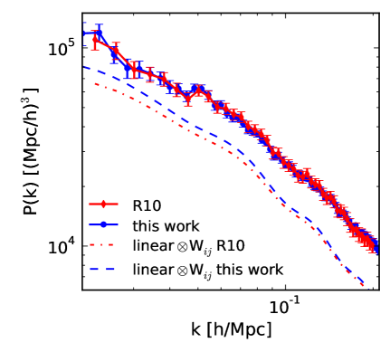
The tension between the constraints obtained when using different measurements, instead, points in the direction of differences in the shape of the power spectrum or of the window matrix. Figure 19 shows the LRG power spectrum described in Section 3.1 (with blue points) and the halo one from R10 (red diamonds). The error-bars show the corresponding variances. Besides a factor of about four in the amplitude, due to the different samples and estimators used, which we include in the figure, the shapes of the two power spectra are almost identical, as we expect. We would also expect the window functions to be similar, but Figure 20 shows that the rows of corresponding to the -bands of the measured power spectra are substantially different. This is intriguing, given that the bulk of our and R10 samples the same. This difference is even clearer when convolving a model with the window function. The dashed and dot-dashed lines in Figure 19 show the best fit linear power spectrum from Figure 2 after the convolution with our and R10 , respectively. In order to avoid clutter the amplitude of these two power spectra is not matched to . The differences in the window matrix are transformed into different shapes of the convolved , which implies that these measurements cannot be described by the same set of cosmological parameters. This difference in the window matrix is responsible for the main differences shown in Table 10.
7.2 Other works
Percival et al. (2010) analysed almost 900,000 galaxies from the combination of the full SDSS DR7 galaxy sample and the two-degree Field Galaxy Redshift Survey (2dFGRS, , 2003) and extracted the BAO feature from the power spectrum in 7 redshift bins. The main cosmological results are shown in their table 5 and can be compared with the third column in Tables 3, 5 and 6 and with Table 8. Their constraints are compatible with ours and with the findings of R10. Significantly, despite the much smaller sample that we use, the constraints that we obtain are comparable or tighter than the ones of Percival et al. (2010). As an example, for the wCDM case we obtain from CMB+ , while they report the value , which corresponds to an improvement of about 25% in our results. This comparison suggests the importance of the use of the full information content in the galaxy power spectrum, as already noticed by different authors (e.g., Sánchez, Baugh & Angulo, 2008; Shoji, Jeong & Komatsu, 2009; , 2011).
The correlation function has also been intensively used with similar goals. Sánchez et al. (2009) applied a model equivalent to the one presented in section 5.1 (Crocce & Scoccimarro, 2008; Sánchez, Baugh & Angulo, 2008) to the correlation function of the LRG sample from the SDSS DR6, as measured by Cabré & Gaztañaga (2009a). Combining this with Union SNIa sample and the CMB measurements from WMAP5, as well as with the position of the BAO peak along the line of sight in the two-dimensional correlation function from (2009), they extracted cosmological parameters for the same parameter spaces presented in this work. The overall results of Sánchez et al. (2009) are consistent with the ones presented in section 6. Interestingly our errors on the cosmological parameters are systematically smaller when curvature is kept as free variable and larger for the wCDM and waCDM cases. This shows that the models and the measurements of the power spectrum and the correlation function, although generally coherent, show some small differences in the sensitivity to cosmological parameters for different parameter spaces. In the kwCDM case, the constraints of Sánchez et al. (2009) show the same bias-shape degeneracy that shifts the values of and upwards with respect to the flat CDM paradigm (compare Figure 14 with figure 14 in Sánchez et al. (2009)). The inclusion of SNIa and of H0 (radial BAO) in our (their) analysis leads to the tightest constraints in both works. For flat and non flat CDM, the differences are negligible, while for the other three cases, where SNIa measurements play an important role, the errors that we obtain are larger: this is due to the inclusion of the supernovae systematic errors, which where neglected in Sánchez et al. (2009), in our analysis. When we do not use the systematics, we obtain tighter constraints, shown by the middle column of Table 7. In this case we measure the dark energy equation of state parameter to be , about 11% tighter than the corresponding value measured by Sánchez et al. (2009, ).
A more recent analysis of the correlation function from the DR7 LRG sample has been made by (2010), using a simplified version of the model presented by Reid et al. (2010). They combined this measurement with WMAP7 and Union2 data in order to extract cosmological parameters. Some of their constraints are offset by 1-2 with respect to our findings and their measurements of the dark energy equation of state are compatible with ours, once the SNIa systematics are neglected. (2011) measured the angular correlation function and detected the BAO feature from the LRGs in the SDSS DR7 photometric catalogue, which consists of a sample of about 1.5 million galaxies. Fixing all the other parameters, with the exception of , to the best fit from WMAP7, they measure to be .
The small scale clustering has Also been used to perform cosmological analyses. From the small scale projected correlation function and mass-number ratio in clusters, modelled in the halo model framework, (2011) extracted cosmological and model parameters, obtaining, when combining with WMAP7, and . The difference between these results and the values of Table 3 might be due to the smaller number of cosmological degrees of freedom and the higher number of model parameters.
In a recent article (2011) presented the first cosmological results from the WiggleZ survey (, 2010). They used a sample of about 130,000 emission line galaxies across 1000 deg2 in the redshift range . From the correlation function, the power spectrum, the BAOs and the band-filtered correlation function (, 2010) they extracted BAO parameters, like the effective distance of equation (15) and the “acoustic parameter”, defined by (, 2005). From those, they measured cosmological parameters for the kCMD and the wCDM models. When using LSS information only, the uncertainties are large but the results show a strong preference for the presence of dark energy, with . Combining the BAO parameters with WMAP7 distance priors they measured the dark energy equation of state parameter to be , which became if also Union2 SN are used. Those results are in agreement with ours, although their uncertainties are about 20-30% larger than the ones that we show in Table 6. The agreement between our results and the ones in (2011) show that, despite the differences in the galaxies selected, the survey volume and geometry and the procedure used to extract cosmological information, both analyses are robust enough for the precision achievable today.
8 Summary and conclusions
We have computed the power spectrum of the distribution of about 90,000 luminous red galaxies, extracted from the spectroscopic part of the seventh data release of the Sloan Digital Sky survey. To compute the covariance matrix for the power spectrum we make use of the 160 LasDamas mock catalogues, which have the same angular and redshift distribution as the observed LRGs. We describe the measured power spectrum with a model inspired by renormalised perturbation theory and modified in order to describe biased objects in redshift space (section 5.1). This model has been successfully tested against numerical simulations (M10) and mock catalogues (section 5.4) for at z=0-0.5.
Combining the large scale structure information with measurements of the CMB temperature and polarisation power spectrum from the seven year data release of WMAP, ACBAR, BOOMERanG, CBI and QUAD and with the luminosity-distance relation from the Union2 supernovae sample and using a precise determination of the local Hubble parameter as a gaussian prior, we explore the constraints in five different cosmological parameter spaces described in section 5.2. They are the flat CDM concordance model, a similar one where curvature is a free parameter (kCDM) and three models in which the dark energy equation of state has a parametric form: in two cases it is assumed to be constant, with and without the assumption of a flat geometry (wCDM and kwCDM), and in the last case (waCDM) we model with the simple parametric formula of equation (9).
Overall, we obtain tight constraints on the cosmological parameters for all the five cases and we do not detect deviations from the flat CDM paradigm. The different combinations of the four experiments used in this analysis do not show any evidence of tensions between cosmological probes. We find that the curvature is null at 1- level with errors of the order of . We measure the dark energy equation of state parameter to be consistent with a cosmological constant with 13% uncertainty for CMB+ and 6.5% uncertainty for CMB+++SNIa in the flat wCDM case. If we discard the systematic errors in the SNIa, the precision increases to 4.6%. In the kwCDM, because of the added degree of freedom, we have a degradation of the constraints to 8.4%, when combining all the four samples. The constraints obtained with the CMB and large scale structure together are shifted by 1.5-2 with respect to the best fit CDM because of a bias-shape degeneracy in the power spectrum that allows very large, and unphysical, values of the bias when , , increase and decreases. If we assume the parametric form of equation (9) for the dark energy equation of state, we obtain (CMB+) and (all four experiments combined). The latter is only slightly worse than the flat wCDM result.
In the near future new and larger galaxy redshift catalogues both spectroscopic, like BOSS and HETDEX, and photometric, like Pan-STARRS and DES, will become available, together with the new measurements of the CMB anisotropies from the Planck satellite (, 2011). These datasets will enable us to improve the constraints presented in this work even further. Some of these experiments are explicitly designed in order to extract the maximum amount of information regarding dark energy. This would allow to exclude many classes of dark energy models or of modifications of general relativity. In order to use the full information from the power of these new large scale observations and to avoid introducing systematic effects, accurate models of the large scale distribution, scale dependent bias and redshift space distortions are necessary. In M10 we showed that the model used in this work is accurate enough to describe the power spectrum shape also for surveys with volumes larger than available nowadays. The explicit inclusion of bias and redshift space distortions in the model would allow however to use a larger range of scales than now possible, helping to improve the quality of the cosmological constrains even further.
Acknowledgments
We thank the LasDamas project for releasing publicly the mock catalogues. We thank Shaun Cole and Andrés Balaguera-Antolínez for discussions about the power spectrum computation and Friedrich Röpke and Sandra Benitez for the clarifications about SNIa. FM acknowledges support by the Trans-regional Collaborative Research Centre TRR33 The Dark Universe of the German Research Foundation (DFG).
Funding for the SDSS and SDSS-II has been provided by the Alfred P. Sloan Foundation, the Participating Institutions, the National Science Foundation, the U.S. Department of Energy, the National Aeronautics and Space Administration, the Japanese Monbukagakusho, the Max Planck Society, and the Higher Education Funding Council for England. The SDSS Web Site is http://www.sdss.org/.
The SDSS is managed by the Astrophysical Research Consortium for the Participating Institutions. The Participating Institutions are the American Museum of Natural History, Astrophysical Institute Potsdam, University of Basel, University of Cambridge, Case Western Reserve University, University of Chicago, Drexel University, Fermilab, the Institute for Advanced Study, the Japan Participation Group, Johns Hopkins University, the Joint Institute for Nuclear Astrophysics, the Kavli Institute for Particle Astrophysics and Cosmology, the Korean Scientist Group, the Chinese Academy of Sciences (LAMOST), Los Alamos National Laboratory, the Max-Planck-Institute for Astronomy (MPIA), the Max-Planck-Institute for Astrophysics (MPA), New Mexico State University, Ohio State University, University of Pittsburgh, University of Portsmouth, Princeton University, the United States Naval Observatory, and the University of Washington.
References
- Abazajian et al. (2009) Abazajian, K. N., et al., 2009, ApJS, 182, 543
- Abbott et al. (2005) Abbott T. et al., 2005, preprint (arXiv:astro-ph/0510346)
- (3) Ade P. A. R. et al., 2011, preprint (arXiv:1101.2022)
- (4) Amanullah R. et al., 2010, ApJ, 716, 712
- (5) Albrecht A. et al., 2006, preprint (arXiv:astro-ph/0609591)
- Angulo et al. (2008) Angulo R., Baugh C. M., Frenk C. S., Lacey C. G., 2008, MNRAS, 383, 755
- (7) Astier P. et al., 2006, A&A, 447, 31
- (8) Balaguera-Antolínez A., Sánchez A. G., Böhringer H., Collins C., Guzzo L., Phleps S., 2011, MNRAS, in press
- (9) Bengochea G. R., 2011, PhLB, 696, 5
- (10) Berlind A. A., Weinberg D. H., 2002, ApJ, 575, 587
- Bernardeau et al. (2002) Bernardeau F., Colombi S., Gaztañaga, E., Scoccimarro R., 2002, PhR, 367, 1
- Bernardeau, Crocce & Scoccimarro (2008) Bernardeau F., Crocce M., Scoccimarro R., 2008, PhRvD, 78, 10352
- (13) Blake C. et al., 2011, arXiv, arXiv:1105.2862
- (14) Brown M. L. et al., 2009, ApJ, 705, 978
- Cabré & Gaztañaga (2009a) Cabré A., Gaztañaga E., 2009, MNRAS, 393, 1183
- (16) Cabré A., Gaztañaga E., 2009, MNRAS, 396, 1119
- (17) Carnero A., Sanchez E., Crocce M., Cabre A., Gaztanaga E., 2011, preprint (arXiv:1104.5426)
- (18) Chevallier M., Polarski D., 2001, IJMPD, 10, 213
- (19) Chuang C.-H., Wang Y., Hemantha M. D. P., 2010, preprint (arXiv:1008.4822)
- Cole et al. (2005) Cole S. et al., 2005, MNRAS, 362, 505
- (21) Coles P., Jones B., 1991, MNRAS, 248, 1
- (22) Colless M. et al., 2003, preprint ( arXiv:astro-ph/030658)
- Cooray & Sheth (2002) Cooray A., Sheth R., 2002, PhR, 372, 1
- Christensen & Meyer (2000) Christensen N., Meyer R., preprint (arXiv:astro-ph/0006401)
- Crocce & Scoccimarro (2006a) Crocce M., Scoccimarro R., 2006, Phys. Rev. D, 73, 063519
- Crocce & Scoccimarro (2006b) Crocce M., Scoccimarro R., 2006, Phys. Rev. D, 73, 063520
- Crocce & Scoccimarro (2008) Crocce M., Scoccimarro R., 2008, Phys. Rev. D, 77, 023533
- (28) Davis M., Geller M. J., 1976, ApJ, 208, 13
- Davis et al. (1985) Davis M., Efstathiou G., Frenk C. S., White S. D. M., 1985, ApJ, 292, 371
- (30) Drinkwater M. J. et al., 2010, MNRAS, 401, 1429
- (31) Dunkley J. et al., 2009, ApJS, 180, 306
- Efstathiou et al. (2002) Efstathiou G. et al., 2002, MNRAS, 330, L29
- Eisenstein & Hu (1998) Eisenstein D. J., Hu W., 1998, ApJ, 496, 605
- Eisenstein & Hu (1999) Eisenstein D. J., Hu W., 1998, ApJ. 511, 5
- Eisenstein et al. (2001) Eisenstein D. J. et al., 2001, AJ, 122, 2267
- (36) Eisenstein D. J. et al., 2005, ApJ, 633, 560
- (37) Eisenstein D. J. et al., 2011, preprint (arXiv:1101.1529)
- (38) Elia A., Kulkarni S., Porciani C., Pietroni M., Matarrese S., 2010, preprint (arXiv:1012.4833)
- Fang, Hu & Lewis (2008) Fang W., Hu W., Lewis A., 2008, PhRvD, 78, 087303
- (40) Feldman H. A., Kaiser N., Peacock J. A., 1994, ApJ, 426, 23
- (41) Frieman J. A. et al., 2008, AJ, 135, 338
- Frigo & Johnson (2005) Frigo M., Johnson S. G., 2005, Proceedings of the IEEE, 93, 216
- (43) Gaztañaga E., Cabré A., Hui L., 2009, MNRAS, 399, 1663
- Gelman & Rubin (1992) Gelman A., Rubin D. B., 1992, Stat. Sci., 7, 457
- Gilks, Richardson & Spiegelhalter (1996) Gilks W. R., Richardson S., Spiegelhalter, D. J., 1996, MarkovChain Monte Carlo in Practice. Chapman and Hall, London, UK
- (46) Guy J. et al., 2007, A&A, 466, 11
- (47) Heitmann K., White M., Wagner C., Habib S., Higdon D., 2010, ApJ, 715, 104
- (48) Hicken M., Wood-Vasey W. M., Blondin S., Challis P., Jha S., Kelly P. L., Rest A., Kirshner R. P., 2009, ApJ, 700, 1097
- Hill et al (2004) Hill G. J., Gebhardt K., Komatsu E. & MacQueen P. J., 2004, The New Cosmology: Conference on Strings and Cosmology, 743, 224
- (50) Hinshaw G. et al., 2003, ApJS, 148, 135
- (51) Holsclaw T., Alam U., Sansó B., Lee H., Heitmann K., Habib S., Higdon D., 2010, PhRvD, 82, 103502
- (52) Hu W., Jain B., 2004, PhRvD, 70, 043009
- Huff et al. (2007) Huff E., Schulz A. E., White M., Schlegel D. J., Warren M. S., 2007, APh, 26, 351
- (54) Huterer D., Starkman G., 2003, PhRvL, 90, 031301
- (55) Huterer D., Turner M. S., 2001, PhRvD, 64, 123527
- (56) Jarosik N. et al., 2010, preprint (arXiv:1001.4744)
- (57) Jha S., Riess A. G., Kirshner R. P., 2007, ApJ, 659, 122
- (58) Jennings E., Baugh C. M., Pascoli S., 2011, MNRAS, 410, 2081
- Jeong & Komatsu (2006) Jeong D., Komatsu E., 2006, ApJ, 651, 619
- Jeong & Komatsu (2009) Jeong D., Komatsu E., 2009, ApJ, 691, 569
- (61) Jones W. C. et al., 2006, ApJ, 647, 823
- Kaiser et al. (2002) Kaiser N. et al., 2002, SPIE, 4836, 154
- (63) Kazin E. A. et al., 2010, ApJ, 710, 1444
- (64) Kessler R. et al., 2009, ApJS, 185, 32
- Komatsu et al. (2009) Komatsu E. et al., 2009, ApJS, 180, 330
- (66) Komatsu E. et al., 2011, ApJS, 192, 18
- Kowalski et al. (2008) Kowalski M. et al, 2008, ApJ, 686, 749
- (68) Kuo C. L. et al., 2007, ApJ, 664, 687
- (69) Larson D. et al., 2011, ApJS, 192, 16
- (70) Laureijs R., 2009, preprint (arXiv:0912.0914)
- Lewis & Bridle (2002) Lewis A., Bridle A., 2002, Phys. Rev. D, 66, 103511
- (72) Lewis A., Challinor A., Lasenby A., 2000, ApJ, 538, 473
- (73) Linder E. V., 2003, PhRvL, 90, 091301
- McDonald (2006) McDonald P., Phys. Rev. D, 2006, 74, 103512
- McDonald (2007) McDonald P., Phys. Rev. D, 2007, 75, 043514
- (76) MacTavish C. J. et al., 2006, ApJ, 647, 799
- Masjedi (2006) Masjedi M. et al., 2006, ApJ, 644, 54
- Matarrese & Pietroni (2007) Matarrese S., Pietroni M., 2007, JCAP, 06, 26
- Matarrese & Pietroni (2008) Matarrese S., Pietroni M., 2008, Mod. Phys. Lett. A, 23, 25
- Matsubara (2004) Matsubara T., 2004, ApJ, 615, 573
- Matsubara (2008a) Matsubara T., 2008, Phys. Rev. D, 77, 063530
- Matsubara (2008b) Matsubara T., 2008, Phys. Rev. D, 78, 083519
- Montesano, Sánchez & Phleps (2010) Montesano F., Sánchez A. G., Phleps S., 2010, MNRAS, 408, 2397
- (84) Montroy T. E. et al., 2006, ApJ, 647, 813
- (85) Moresco M., Jimenez R., Cimatti A., Pozzetti L., 2010, preprint (arXiv:1010.0831)
- (86) Norberg P. et al., 2001, MNRAS, 328, 64
- (87) Norberg P. et al., 2002, MNRAS, 332, 827
- (88) Peebles P. J. E., Yu J. T., 1970, ApJ, 162, 815
- (89) Peebles P. J., Ratra B., 2003, Rev. Mod. Phys., 75, 559
- Percival et al. (2002) Percival W. J. et al.,2002, MNRAS, 337, 1068
- (91) Percival W. J., Verde L., Peacock J. A., 2004, MNRAS, 347, 645
- Percival et al. (2007) Percival W.J., Cole S., Eisenstein D. J., Nichol R. C., Peacock J. A., Pope A. C., Szalay A. S., 2007, MNRAS, 381, 1053
- Percival et al. (2010) Percival W. J. et al., 2010, MNRAS, 401, 2148
- Perlmutter et al. (1999) Perlmutter S. et al., 1999, ApJ, 517, 565
- Phleps et al. (2006) Phleps S., Peacock J. A., Meisenheimer K., Wolf C., 2006, A&A, 457, 145
- (96) Piacentini F. et al., 2006, ApJ, 647, 833
- Pietroni (2008) Pietroni M., 2008, JCAP, 10, 36
- (98) Reichardt C. L. et al., 2009, ApJ, 694, 1200
- Reid & Spergel (2009) Reid B. A., Spergel D. N., 2009, ApJ, 698, 143
- (100) Reid B. A., White M., 2011, preprint (arXiv:1105.4165)
- Reid et al. (2009) Reid B. A., Spergel D. N., Bode P., 2009, ApJ, 702, 249f
- Reid et al. (2010) Reid B. A. et al., 2010, MNRAS, 404, 60
- Riess et al. (1998) Riess A. G. et al., 1998, AJ, 116, 1009
- (104) Riess A. G. et al., 2004, ApJ, 607, 665
- (105) Riess A. G. et al., 2007, ApJ, 659, 98
- (106) Riess A. G. et al., 2009, ApJ, 699, 539
- (107) Riess A. G., et al., 2011, ApJ, 730, 119
- (108) Samushia L., Percival W. J., Raccanelli A., 2011, preprint(arXiv:1102.1014)
- Sánchez & Cole (2008) Sánchez A. G., Cole S., 2008, MNRAS, 385, 830
- Sánchez et al. (2006) Sánchez A. G., Baugh C. M., Percival W. J., Peacock J. A., Padilla N. D., Cole S., Frenk C. S., Norberg P., 2006, MNRAS, 366, 189
- Sánchez, Baugh & Angulo (2008) Sánchez A. G., Baugh C. M., Angulo, R., 2008, MNRAS, 390, 1470
- Sánchez et al. (2009) Sánchez A. G., Crocce M., Cabre A., Baugh C. M., Gaztanaga E., 2009, MNRAS., 400. 1643
- Schlegel, White & Eisenstein (2009) Schlegel D., White M., Eisenstein D., 2009, preprint( arXiv:0902.4680)
- Scoccimarro (2004) Scoccimarro R., 2004, Phys. Rev. D, 70, 083007
- (115) Serra P., Cooray A., Holz D. E., Melchiorri A., Pandolfi S., Sarkar D., 2009, Phys. Rev. D, 80, 121302
- Shoji, Jeong & Komatsu (2009) Shoji M., Jeong D., Komatsu E., 2009, ApJ, 693, 1404
- (117) Sievers J. L. et al., 2009, preprint (arXiv:0901.4540)
- (118) Smith R. E. et al., 2003, MNRAS, 341, 1311
- (119) Smith R. E., Scoccimarro R., Sheth R. K., 2008, PhRvD, 77, 043525
- Smith, Hernández-Monteagudo & Seljak (2009) Smith R., Hernández-Monteagudo C., Seljak U., Phys. Rev. D, 2009, 80, 063528
- Spergel et al. (2003) Spergel D. N. et al., 2003, ApJS, 148, 175
- Spergel et al. (2007) Spergel D. N. et al., 2007, ApJS, 170, 377
- Sugiyama (1995) Sugiyama N., 1995, ApJS, 100, 28
- (124) Sunyaev R. A., Zeldovich Y. B., 1970, Ap&SS, 7, 3
- Taruya & Hiramatsu (2008) Taruya A., Hiramatsu T., 2008, ApJ, 674, 617
- (126) Taruya A., Nishimichi T., Saito S., Hiramatsu T., 2009, PhRvD, 80, 123503
- (127) Taruya A., Nishimichi T., Saito S., 2010, PhRvD, 82, 063522
- (128) Tegmark M., Silk J., Blanchard A., 1994, ApJ, 420, 484
- Tegmark et al. (2004) Tegmark M. et al., 2004, ApJ 606, 702
- (130) Tinker J. L. et al., 2011, preprint (arXiv:1104.1635)
- (131) Tsujikawa S., 2010, LNP, 800, 99
- (132) Vikhlinin A. et al., 2009, ApJ, 692, 1060
- (133) Wood-Vasey W. M. et al., 2007, ApJ, 666, 694
- (134) Xu X. et al., 2010, ApJ, 718, 1224
- (135) Zehavi I. et al., 2002, ApJ, 571, 172
Appendix A Basic equations to compute the power spectrum
In this section we summarise the basic equations of the FKP and PVP estimators used to compute the power spectrum and the window function from galaxy surveys. PVP is a generalisation of FKP and takes in account the change of the galaxy bias with the luminosity of the galaxies (see e.g., , 1976, 2001, 2002, 2002; Phleps et al., 2006).
The observed power spectrum is obtained from the squared average Fourier transform of the weighted density field defined by
| (17a) | |||
| (17b) |
where and are the number density of galaxies and randoms of luminosity at position . The corresponding quantities of equation (17a) can be obtained integrating over the luminosity. , are weighting functions and , only PVP, is the bias relative to a specific galaxy population with luminosity . The normalisation is defined by
| (18a) | |||
| (18b) |
where and are, respectively, the mean expected number density, i.e. in absence of clustering, of galaxies of luminosity at position and its integral over . Finally is a constant introduced to match the two catalogues and is chosen requiring that888In FKP, the authors use a definition of such that . :
| (19a) | |||
| (19b) |
The observed power spectrum can be then written for both estimators as:
| (20) |
where is the “true” underlying power spectrum, the shot noise is given by
| (21a) | |||
| (21b) |
and is the window function, which encodes information about the survey geometry.
It can be shown that the window function is computed from the spherical averaged Fourier transform of the field
| (22a) | |||
| (22b) |
as . is the shot noise defined by
| (23a) | |||
| (23b) |
In this work, we use the weighting functions, designed to minimise the variance, proposed in FKP and Cole et al. (2005):
| (24a) | |||
| (24b) |
The intrinsic weight of the objects, , can contain information about completeness and/or fibre collision (, 2002; Masjedi, 2006). is an estimate of the recovered power spectrum and it is usually substituted with a constant , chosen in order to minimise the variance around the wave-number for which .
Appendix B Impact of weights on power spectra and cosmological constraints
In the following we test the impact of , and estimator on the LRG and mock power spectra, on the errors and on the cosmological parameters.
B.1 Testing the luminous red galaxies power spectrum
In this appendix we test the impact of different choices of the estimator, and on the LRG power spectrum and window function. For both estimators, FKP and PVP, we test four values of . We also consider four different intrinsic weights: i) (all the objects have equal weight), ii) (areas with low completeness have less weight than areas with higher one), iii) (the loss of galaxies due to fibre collisions is compensated as described in Section 3.1) and iv) (both completeness and fibre collision corrections applied).
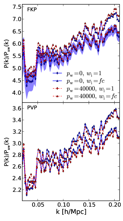
Figure 21 shows the differences in the power spectra measured with the FKP (upper panel) and PVP (lower panel) estimators for the different choices of and . For clarity, in the figure we show only the combination of (red dashed and blue solid lines respectively) and (diamonds and up triangles, respectively). The shaded area shows the standard deviation as measured from the mock catalogues for . All the power spectra have been divided by a non-wiggle one with the same cosmological parameters as the mock catalogues. Different choices of change marginally the shape of the power spectrum. The results for fall in between the two extreme cases shown in Figure 21.
Instead, the correction for fibre collision has a significant effect. When obtaining spectra of crowded fields, not all the objects of interest can be targeted with a limited number of pointings. Because of this loss of objects, the amplitude of the highest peak in the density fields decreases, while the low density regions are unaffected. This causes the amplitude of the fluctuations, and consequently of the power spectrum, to be lower. We have indeed measured a few percent scale independent decrease in the amplitude of (i.e. the power spectrum before subtracting the shot noise) in the case when fibre collision correction is not applied. This difference is visible at the large scale, low , limit in Figure 21 where the power spectrum with the fibre collision (triangles) is always larger than the one without (diamonds). On the other side the shot noise (equations 21) depends on the expected non-clustered number density () and the associated weights, which are not influenced (or influenced in a uniform way) by fibre collisions. This causes the shot noise to be the same in both cases, changing the shape of the final power spectrum . This effect is clearly visible in the small scale, large , limit in Figure 21, where the fibre collision corrected power spectra become increasingly larger than the non corrected ones. We do not show the results when completeness correction is included, since the measured power spectra overlap almost exactly the non corrected ones. This is because both the galaxy and the random catalogues are weighted in the same way, therefore the density fluctuation field is unchanged.
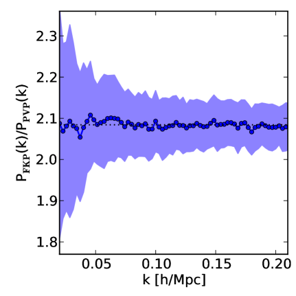
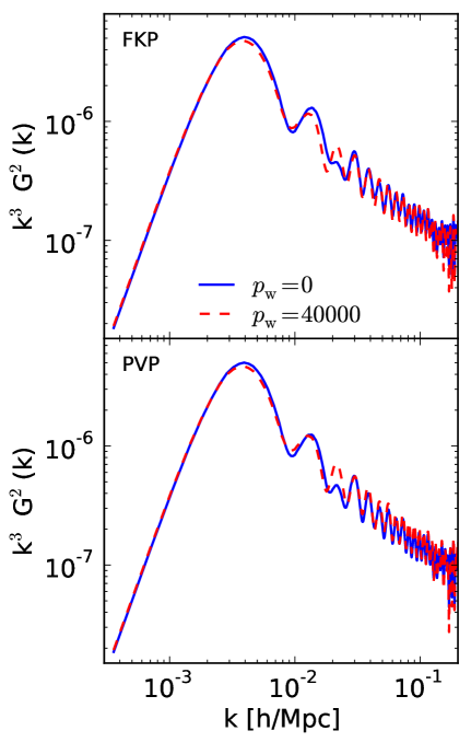
Comparing the two panels of Figure 21, is it clear that the choice of the estimator has a strong impact on the recovered power spectra: in the PVP case the amplitude is systematically lower than for FKP. Figure 22 shows the ratio of the power spectrum computed with the latter estimator with respect to the one computed with the former for the case , . As before, the shaded area corresponds to the standard deviation computed from the LasDamas catalogues. Although the amplitude is different, the relative bias between the two estimators is scale invariant in the range . This is expected from the fact that the galaxy sample that we use is almost volume limited and contains a very uniform population of galaxies.
Recently, (2010) have shown that, in volume limited mock catalogues of the REFLEX II cluster survey, the power spectrum computed with the PVP estimator has higher correlations than the FKP one already at . Because of this and of the scale independent relative bias, we can safely use the power spectra as estimated with FKP in order to constrain cosmological parameters.
The window function, describing only the radial and angular selection function of the survey, is not affected by fibre collision effect; on the other hand different choices of and the completeness correction change the weights of equations (24), which influence the effective survey volume. As for the power spectrum, we do not measure differences when the completeness weighting is applied. Figure 23 shows the “dimensionless” window function computed with FKP (upper panel) and PVP (lower panel) for (dashed and solid line respectively). Although the overall shape is similar, there are small differences in the oscillations due to different effective volumes in the two cases. The results for fall in between the two extreme cases. The difference between the FKP and PVP window functions are negligible.
When convolving these window functions with a linear power spectrum as in equation (1), the differences in the range are negligible.
B.2 Testing the power spectra of the mock catalogues
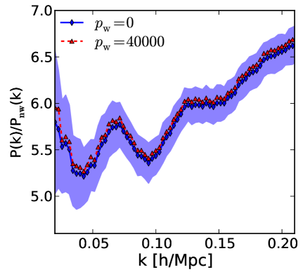
In order to test the impact of on the results from the LasDamas, we compute the power spectra of the 160 mocks, their mean, standard deviation and covariance matrix for . Figure 24 shows the mean power spectra computed for the two extreme cases: the only difference is a small change in amplitude, which confirms the findings of the previous appendix, i.e. that the impact of different on the computed power spectrum is negligible. The shaded area denotes the standard deviation for .
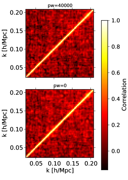
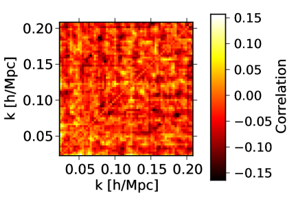
The choice of has, however, a large effect on the errors. Figures 25 and 26 show, respectively, the correlation matrix for (upper panel) and (lower panel) and their difference. At , for we measure that the correlation is systematically, although not significantly, lower than for . This is expected since, when using FKP, . At larger wave-number the power spectrum amplitude is smaller than at and the variance and the correlation are smaller for small values of . This justifies our choice of using in our analysis, since the amplitude of the power spectrum is of this order in the range of scales we are interested in. If the analysis were centred on the small scale power spectrum or correlation function, a smaller value of would be preferable.
B.3 Impact on the cosmological parameters
Here we test how the differences in the shape of the LRG power spectrum and the covariance matrix influence the cosmological parameters measured assuming the wCDM cosmology. We combine the LSS information with the WMAP7 data.
Contrary to our expectations based on the results shown in Appendix B.1, the cosmological parameters are much more sensible to than to . For a fixed the covariance matrix is the same and only the shape of the power spectrum changes. As the shape of the power spectrum is not affected by the completeness correction, also the cosmological constraints are insensitive to it. The fibre collision correction instead changes the bias, over which we marginalise analytically, without affecting the shot noise amplitude. Differences in the relative amplitude of the latter term can be absorbed at least partially by the mode coupling amplitude , which is systematically, although not significantly, larger when the loss of galaxies due to fibre collisions is corrected for. Because of this, cosmological constraints remain almost unchanged for different . Changes of instead influence the covariance but only marginally the power spectrum. The differences in the former influence the cosmological parameters, which differ by , for and 0. For example I obtain the dark energy equation of state parameter to be for and for .
Given the precision that is possible to achieve with the data used in this article, the differences just highlighted are not distinguishable from the uncertainties in the parameters. But in future, given the big improvements expected, these effects might become important and will need further analysis.