Ignition from a Fire Perimeter in a WRF Wildland Fire Model

Abstract

The current WRF-Fire model starts the fire from a given ignition point at a given time. We want to start the model from a given fire perimeter at a given time instead. However, the fuel balance and the state of the atmosphere depend on the history of the fire. The purpose of this work is to create an approximate artificial history of the fire based on the given fire perimeter and time and an approximate ignition point and time. Replaying the fire history then establishes a reasonable fuel balance and outputs heat fluxes into the atmospheric model, which allow the atmospheric circulation to develop. Then the coupled atmosphere-fire model takes over. In this preliminary investigation, the ignition times in the fire area are calculated based on the distance from the ignition point to the perimeter, assuming that the perimeter is convex or star-shaped. Simulation results for an ideal example show that the fire can continue in a natural way from the perimeter. Possible extensions include algorithms for more general perimeters and running the fire model backwards in time from the perimeter to create a more realistic history. The model used extends WRF-Fire and it is available from openwfm.org.

1 Introduction

Fire models generally start the fire from a given ignition point at a given time, and sophisticated ignition parameterizations exist, including line ignition and submesh ignition procedures Mandel et al. (2011). However, in practice one is often faced with the need to start a fire model from a fire already in progress. Often only perimeter data pertaining to some time are available, such as from the US Forest Service at activefiremaps.fs.fed.us. This need arizes in analyses of existing fires currently, and it will become even more important for forecasting of the behavior of fires in progress in future.

With models that do not include two-way interaction with the atmosphere, continuing from an existing fire state is essentially straightforward. While the fuel can be partially burned in some areas, fuel in locations untouched by the fire is unchanged, and the model can simply progress to the new areas regardless of the fire history. (A model that may include long-range effects such as preheating in front of the fire, would be an exception.) In a coupled atmosphere-fire model, however, the situation is very different. First, simply igniting the whole area inside the given perimeter is not an option, because the large instantaneous heat release will cause the model to break down. More importantly, the state of the atmosphere evolves in interaction with the fire, and the buyoancy caused by the heat flux causes significant changes to the wind field, which in turn influences the future progress of the fire.

Starting the fire from a state already developed is essentially a data assimilation problem, and it could be treated as such by a shooting method: the fire starts from a ignition point at a time in the past, then at the given simulation time, the state of the fire is compared with the given perimeter, and adjustments can be made to the ignition time and location, much as in variational data assimilation methods such as 4DVAR. We plan to study such approaches in future as a part of our effort in the area of data assimilation for wildland fires Beezley (2009); Beezley and Mandel (2008); Mandel et al. (2008, 2009, 2010).

The approach adopted here is different. Given a fire perimeter, we create an artificial history. Then the fire history is replayed, which produces heat output into the atmosphere, and the atmospheric model spins up to a state that is plausible for the fire at the stage given by the perimeter. The artificial history is essentially a parameterization of the process that leads to the development of the fire perimeter. Parameterizations of various levels of sophistication can be considered, up to and including running a fire model backwards in time to find an ignition point and iterating to find a matching atmospheric state. In this initial study, we consider a very simple artificial history model, and show that it results in acceptable fire and atmosphere states for the perimeter. Approximate perimeter states obtained by such method could provide also a good starting point for data assimilation in future.

2 The model

Fire models range from tools based on Rothermel (1972) fire spread rate formulas, such as BehavePlus (Andrews 2007) and FARSITE (Finney 1998), suitable for operational forecasting, to sophisticated 3-D computational fluid dynamics and combustion simulations suitable for research and reanalysis, such as FIRETEC (Linn et al. 2002) and WFDS (Mell et al. 2007). BehavePlus, the PC-based successor of the calculator-based BEHAVE, determines the fire spread rate at a single point from fuel and environmental data; FARSITE uses the fire spread rate to provide a 2-D simulation on a PC; while FIRETEC and WFDS model combustion in 3D, which is much more expensive. See the survey by Sullivan (2009) for a number of other models.

The model considered here couples the mesoscale atmospheric code WRF-ARW Skamarock et al. (2008) with a fire spread module, based on the Rothermel model Rothermel (1972) and implemented by the level set method. In each time step, the fire model inputs the atmospheric winds and outputs surface sensible and latent heat fluxes into the atmosphere. Only the finest domain in WRF is coupled with the fire model. The fire model works in conjunction with WRF land use models, and it interpolates horizontal winds from the ideal logarighmic wind profile to appropriate heights above the surface, for each fuel.

The model has grown out of NCAR’s CAWFE code Clark et al. (1996b, a, 2004); Coen (2005), which couples the Clark-Hall atmospheric model with fire spread implemented by tracers, and it got its start from a prototype code coupling the fire model in CAWFE with WRF in LES mode Patton and Coen (2004). The tracers, however, were replaced by a level set method, which we considered more flexible and more suitable for data assimilation and WRF parallel infrastructure. The coupled model is capable of running faster than real time in LES mode, with resolution of tens of meters for the atmosphere, and meters for the fire, with the matching time step of a fraction of a second, on the innermost modeling domain of many kilometers in size Jordanov et al. (2011). Fuel data and topography can be obtained from government databases in the United States and from satellite images and GIS elsewhere Jordanov et al. (2011). See Mandel et al. (2009, 2011) for futher details and references. The model is currently available from the Open Wildland Fire Modeling environment at openwfm.org, along with utilities for data preparation, visualization, and diagnostics and a wiki with many user guides for the specific features and utilities, discussion, and support. A code containing a subset of the features is distributed with WRF as WRF-Fire.

3 Encoding and replaying the fire history

The state of the fire model consists of a level set function, $\Phi$, given by its values on the nodes of the fire model mesh, and time of ignition $T_{\mathrm{i}}$. The level set function is interpolated linearly. At a given simulation time $t$, the fire area is the set of all points $\left(x,y\right)$ where $\Phi\left(t,x,y\right)\leq 0$. The level set function and the ignition time satisfy the consistency condition

$$\Phi\left(t,x,y\right)\leq 0\Longleftrightarrow T_{\mathrm{i}}\left(x,y\right)\leq t,$$ (1)

as both of these inequalities express the condition that the location $\left(x,y\right)$ is burning at the time $t$. In every time step of the simulation, the level set function is advanced by one step of a Runge-Kutta scheme for the level set equation

$$\frac{d\Phi}{dt}=-R\left\|\nabla\Phi\right\|,$$

where $R=R\left(t,x,y\right)$ is the fire rate of spread, which depends on the fuel, wind speed, and slope. The ignition time at nodes is then computed for all newly ignited nodes, and it satisfies the consistency condition (1).

The fire history is encoded as an array of ignition times $T_{\mathrm{i}}\left(x,y\right)$, prescribed at all fire mesh nodes. To replay the fire in the period $0\leq t\leq T_{\mathrm{per}}$, the numerical scheme for advancing $\Phi$ and $T_{\mathrm{i}}$ is suspended, and instead the level set function is set to

$$\Phi\left(t,x,y\right)=T_{\mathrm{i}}\left(x,y\right)-t.$$

After the end of the replay is reached, the numerical scheme of the level set method is started from the level set function $\Phi$ at $t=T_{\mathrm{per}}$.

For reasons of numerical accuracy and stability, the level set function needs to have approximately uniform slope. For example, a very good level set function, which has slope equal to one, is the signed distance from a given closed curve $\Gamma$,

$$\Phi\left(x,y\right)=\pm\operatorname*{dist}\left(\left(x,y\right),\Gamma\right),$$

where the sign is taken to be negative inside the region limited by $\Gamma$, and positive outside Osher and Fedkiw (2003). Thus, the ignition times $T_{\mathrm{i}}$ need to be given on the whole domain and they need to be such that $T_{\mathrm{i}}$ decreases with the distance from the given perimeter inside the fire region, and increases outside. The ignition times $T_{\mathrm{i}}$ outside of the given fire perimeter are perhaps best thought of as what the ignition times might be in future as the fire keeps burning.

4 Creating an artificial fire history

The purpose of this algorithm is to create the artificial values of the time of ignition on the fire model mesh, given ignition point ($x_{\mathrm{ign}}$, $y_{\mathrm{ign}}$), ignition time $T_{\mathrm{ign}}$, fire perimeter $\Gamma$, and the time when the fire reached the perimeter $T_{\mathrm{per}}$, assuming that the fire perimeter is convex, or at least star-shaped with respect to the ignition point. The fire perimeter is given as a set of points $(x_{k},y_{k})$ in the fire model domain, $k=1,\ldots,n$ which form a closed curve consisting of line segments $\left[(x_{k},y_{k}),(x_{k+1},y_{k+1})\right]$ between each two successive points. We take $(x_{1},y_{1})=(x_{n+1},y_{n+1})$ so that the starting and the ending point are identical. The coordinates of the point of ignition and of the points defining of the fire perimeter do not need to coincide with mesh points of the grid.

The method consists of linear interpolation of the ignition time between $T_{\mathrm{ign}}$ at the ignition point and $T_{\mathrm{per}}$ on the perimeter, along straight lines connecting the ignition point with points on the perimeter. The ignition time is also extrapolated beyond the perimeter in the same manner to provide a suitable level set function, as discussed in the previous section. Given a mesh point with coordinates $\left(x,y\right)$, the algorithm to determine the ignition time $T_{\mathrm{i}}\left(x,y\right)$ consists of the following steps.

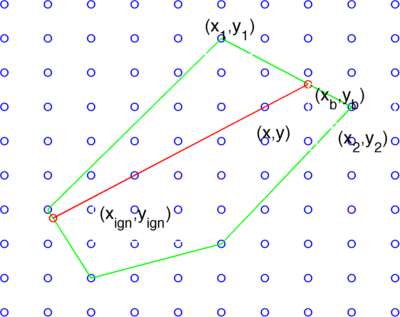
1. Find the intersection $\left(x_{\mathrm{b}},y_{\mathrm{b}}\right)$ of the fire perimeter and the half-line starting at the ignition point and passing through the point $\left(x,y\right)$ (Fig. 1). For this purpose, we use the function

   $$F(x,y,x_{b},y_{b})=(y_{b}-y_{\mathrm{ign}})(x-x_{\mathrm{ign}})-(x_{b}-x_{\mathrm{ign}})(y-y_{\mathrm{ign}}),$$

   which is zero if point $\left(x_{\mathrm{b}},y_{\mathrm{b}}\right)$ lies on the line defined by $(x,y)$ and $(x_{\mathrm{ign}},y_{\mathrm{ign}})$, and it is positive in one half-plane and negative in the other. We then find segment $\left[(x_{k},y_{k}),(x_{k+1},y_{k+1})\right]$ such that $F(x,y,x_{k},y_{k})F(x,y,x_{k+1},y_{k+1})<0$, that is, the points $(x_{k},y_{k})$ and $(x_{k+1},y_{k+1})$ lie on opposite sides of the line passing through $(x,y)$ and $(x_{\mathrm{ign}},y_{\mathrm{ign}})$. Since the line intersects the fire perimeter at two points, one on each side of the ignition point, we choose correct segment as follows:

   • If $\left(x,y\right)$ is inside $\Gamma$, that is, closer to the ignition point than to the intersection, then the desired segment is the one that lies on the same side from the ignition point as the point $\left(x,y\right)$;

   • If $\left(x,y\right)$ is outside of $\Gamma$, then the needed segment lies on the same side from the ignition point as $\left(x,y\right)$.

2. Calculate the time of ignition of the mesh point, based on the ratio of the distances of the mesh point and the perimeter point to the ignition point,

   $$T_{\mathrm{i}}(x,y)=T_{\mathrm{ign}}+\frac{\left\|\left(x,y\right)-\left(x_{\mathrm{ign}},y_{\mathrm{ign}}\right)\right\|}{\left\|\left(x_{\mathrm{b}},y_{\mathrm{b}}\right)-\left(x_{\mathrm{ign}},y_{\mathrm{ign}}\right)\right\|}\left(T_{\mathrm{per}}-T_{\mathrm{ign}}\right).$$

Figure 1: Construction of intersection of the fire perimeter and the half line originating from the Ignition point and passing through a given mesh point.

5 Computational results

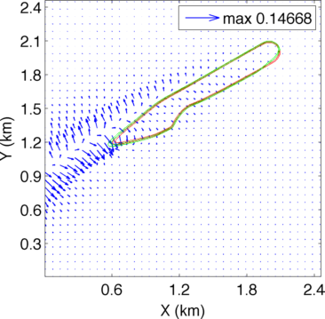
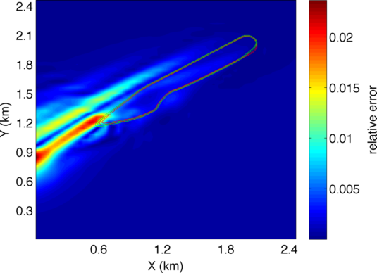
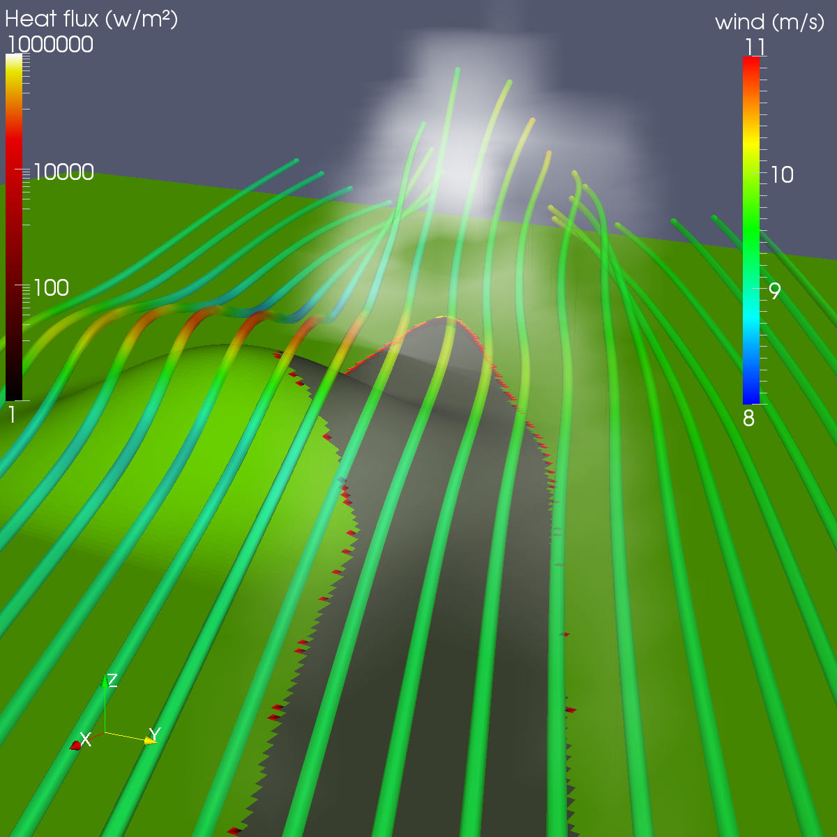
We have tested this algorithm on an ideal example to measure the difference in the atmospheric winds between a simulation propagated naturally from a point and another one advanced artificially. In this example, the topography was flat except for a small hill roughly $500$ m in diameter and $100$ m high in the center of a domain of size $2.4$ km $\times$ $2.4$ km. The atmospheric and fire grid resolutions used were $60$ m and $6$ m respectively, with a $0.25$ s time step. The background winds were approximately $9.5$ m/s traveling southwest at the lowest atmospheric layer $30$ m above the surface. The first simulation was ignited from a point in the northeast corner of the domain $2$ seconds from the start, and the fire perimeter was recorded after $40$ minutes. This perimeter and ignition location were used to generate an artificial history for the first $40$ minutes, which was replayed in the second simulation. Therefore, the fire perimeters in both simulations are identical at $40$ minutes. Both simulations were then allowed to advance another $28$ minutes, using the standard coupled model. The outputs were then collected for analysis.

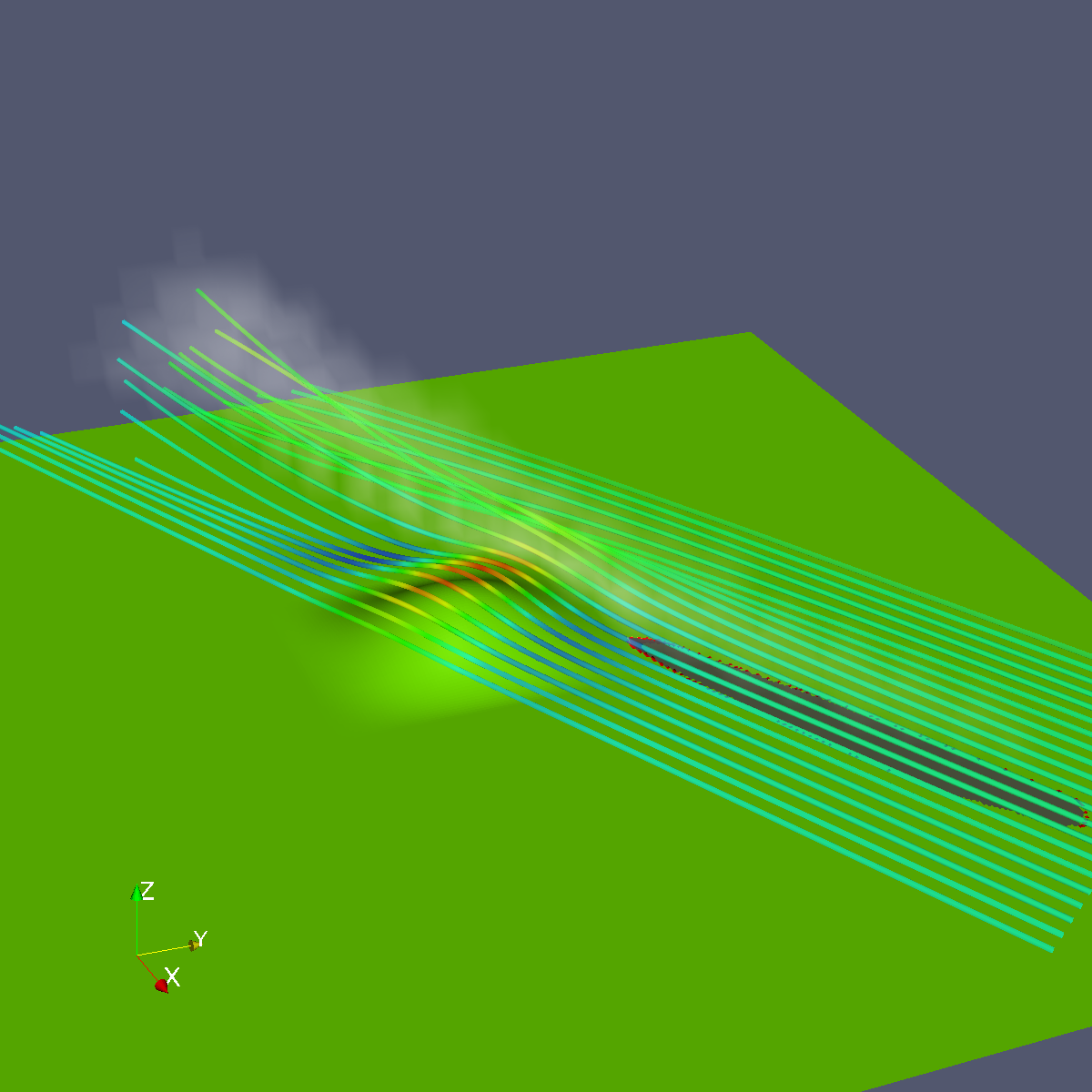
Any differences in the simulations after this time are a result of the error of the artificial fire propagation. In Fig. 3, we show 3D renderings of the simulation. The streamlines near the surface show the updraft created as a result of the heat output from the fire. In Fig. 3a, the fire is affecting the atmosphere despite being propagated artificially. A semi-transparent volume rendering of QVAPOR was added to simulate the smoke release. In Fig. 2, the differences in the wind between the two simulations at $68$ minutes and the fire perimeter are shown. Fig. 2a, shows the difference of the wind from the direct fire propagation minus the wind from the artificial propagation. Fig. 2b shows the relative error in the wind speed defined as the norm of the difference from Fig. 2a, divided by the wind speed from the direct simulation. This shows that the maximum error at the end of this $68$ minute simulation is less than $2.5\%$. In this case, the Froude number is about $F_{c}=0.79$, showing that the heating from the fire may significantly affect ambient wind, therefore small differences caused by using the artificial history have an effect. The effect is concentrated downwind from the fire, as it could be expected.

(a) The difference in the winds of the direct simulation minus the artificial propagation at $68$ minutes.

(b) The relative error in the speed of the wind at $68$ minutes.

Figure 2:

(a) The artificial fire simulation at $40$ minutes.

(b) The direct fire simulation at $68$ minutes.

Figure 3:

6 Conclusion

We have presented a parameterization of the fire up to a point in time when a fire perimeter is given. The parameterization allows for the changes in the atmospheric circulation to develop, caused by the heat flux from the fire. This provides appropriate starting conditions for the computation to continue with the full coupled fire-atmosphere simulation. We have shown on an ideal example that the differences in the state of the atmosphere between a complete fire simulation and when the parameterization is used are not significant. In the studied case, the coupling between the fire and the atmosphere was strong. It would be interesting to observe how the the differences change if the problem moves from the wind-driven ($F_{c}>1$) to the plume driven regime ($F_{c}<1$) regime. This will be studied elsewhere. We plan to study also algorithms for more general domains, not just star-shaped, and to take into account different rates of fire propagation due to fuel nonhomogeneity.

References

- Andrews (2007) Andrews, P. L., 2007: BehavePlus fire modeling system: past, present, and future. Paper J2.1, 7th Symposium on Fire and Forest Meteorology, http://ams.confex.com/ams/pdfpapers/126669.pdf.
- Beezley (2009) Beezley, J. D., 2009: High-Dimensional Data Assimilation and Morphing Ensemble Kalman Filters with Applications in Wildfire Modeling. Ph.D. thesis, University of Colorado Denver.
- Beezley and Mandel (2008) Beezley, J. D. and J. Mandel, 2008: Morphing ensemble Kalman filters. Tellus, 60A, 131–140, doi:10.1111/j.1600-0870.2007.00275.x.
- Clark et al. (2004) Clark, T. L., J. Coen, and D. Latham, 2004: Description of a coupled atmosphere-fire model. International Journal of Wildland Fire, 13, 49–64, doi:10.1071/WF03043.
- Clark et al. (1996a) Clark, T. L., M. A. Jenkins, J. Coen, and D. Packham, 1996a: A coupled atmospheric-fire model: Convective feedback on fire line dynamics. J. Appl. Meteor, 35, 875–901, doi:10.1175/1520-0450(1996)0350875:ACAMCF2.0.CO;2.
- Clark et al. (1996b) Clark, T. L., M. A. Jenkins, J. L. Coen, and D. R. Packham, 1996b: A coupled atmosphere-fire model: Role of the convective Froude number and dynamic fingering at the fireline. International Journal of Wildland Fire, 6, 177–190, doi:10.1071/WF9960177.
- Coen (2005) Coen, J. L., 2005: Simulation of the Big Elk Fire using coupled atmosphere-fire modeling. International Journal of Wildland Fire, 14, 49–59, doi:10.1071/WF04047.
- Finney (1998) Finney, M. A., 1998: FARSITE: Fire area simulator-model development and evaluation. Res. Pap. RMRS-RP-4, Ogden, UT: U.S. Department of Agriculture, Forest Service, Rocky Mountain Research Station, http://www.fs.fed.us/rm/pubs/rmrs_rp004.html.
- Jordanov et al. (2011) Jordanov, G., J. D. Beezley, N. Dobrinkova, A. K. Kochanski, and J. Mandel, 2011: Simulation of the 2009 Harmanli fire (Bulgaria). 8th International Conference on Large-Scale Scientific Computations, Sozopol, Bulgaria, June 6-10, 2011, lecture notes in Computer Science, Springer, to appear.
- Linn et al. (2002) Linn, R., J. Reisner, J. J. Colman, and J. Winterkamp, 2002: Studying wildfire behavior using FIRETEC. Int. J. of Wildland Fire, 11, 233–246, doi:10.1071/WF02007.
- Mandel et al. (2009) Mandel, J., J. D. Beezley, J. L. Coen, and M. Kim, 2009: Data assimilation for wildland fires: Ensemble Kalman filters in coupled atmosphere-surface models. IEEE Control Systems Magazine, 29, 47–65, doi:10.1109/MCS.2009.932224.
- Mandel et al. (2011) Mandel, J., J. D. Beezley, and A. K. Kochanski, 2011: Coupled atmosphere-wildland fire modeling with WRF-Fire version 3.3. Geoscientific Model Development Discussions, 4, 497–545, doi:10.5194/gmdd-4-497-2011.
- Mandel et al. (2010) Mandel, J., J. D. Beezley, and V. Y. Kondratenko, 2010: Fast Fourier transform ensemble Kalman filter with application to a coupled atmosphere-wildland fire model. Computational Intelligence in Business and Economics, Proceedings of MS’10, A. M. Gil-Lafuente and J. M. Merigo, eds., World Scientific, 777–784.
- Mandel et al. (2008) Mandel, J., L. S. Bennethum, J. D. Beezley, J. L. Coen, C. C. Douglas, M. Kim, and A. Vodacek, 2008: A wildland fire model with data assimilation. Mathematics and Computers in Simulation, 79, 584–606, doi:10.1016/j.matcom.2008.03.015.
- Mell et al. (2007) Mell, W., M. A. Jenkins, J. Gould, and P. Cheney, 2007: A physics-based approach to modelling grassland fires. Intl. J. Wildland Fire, 16, 1–22, doi:10.1071/WF06002.
- Osher and Fedkiw (2003) Osher, S. and R. Fedkiw, 2003: Level Set Methods and Dynamic Implicit Surfaces. Springer, New York.
- Patton and Coen (2004) Patton, E. G. and J. L. Coen, 2004: WRF-Fire: A coupled atmosphere-fire module for WRF. Preprints of Joint MM5/Weather Research and Forecasting Model Users’ Workshop, Boulder, CO, June 22–25, NCAR, 221–223, http://www.mmm.ucar.edu/mm5/workshop/ws04/Session9/Patton_Edward.pdf.
- Rothermel (1972) Rothermel, R. C., 1972: A mathematical model for predicting fire spread in wildland fires. USDA Forest Service Research Paper INT-115, http://www.treesearch.fs.fed.us/pubs/32533.
- Skamarock et al. (2008) Skamarock, W. C., J. B. Klemp, J. Dudhia, D. O. Gill, D. M. Barker, M. G. Duda, X.-Y. Huang, W. Wang, and J. G. Powers, 2008: A description of the Advanced Research WRF version 3. NCAR Technical Note 475, http://www.mmm.ucar.edu/wrf/users/docs/arw_v3.pdf.
- Sullivan (2009) Sullivan, A. L., 2009: A review of wildland fire spread modelling, 1990-present, 1: Physical and quasi-physical models, 2: Empirical and quasi-empirical models, 3: Mathematical analogues and simulation models. International Journal of WildLand Fire, 18, 1: 347–368, 2: 369–386, 3: 387–403, doi:10.1071/WF06143, 10.1071/WF06142, 10.1071/WF06144.