Distances and Riemannian metrics
for multivariate spectral densities

Xianhua Jiang, Lipeng Ning, and Tryphon T. Georgiou Supported by NSF, AFOSR, and the Vincentine Hermes-Luh Endowment. The authors are with the Department of Electrical & Computer Engineering, University of Minnesota, Minneapolis, MN 55455. {jiang082, ningx015, tryphon}@umn.edu
Abstract

We first introduce a class of divergence measures between power spectral density matrices. These are derived by comparing the suitability of different models in the context of optimal prediction. Distances between “infinitesimally close” power spectra are quadratic, and hence, they induce a differential-geometric structure. We study the corresponding Riemannian metrics and, for a particular case, provide explicit formulae for the corresponding geodesics and geodesic distances. The close connection between the geometry of power spectra and the geometry of the Fisher-Rao metric is noted.

I Introduction

Distance measures between statistical models and between signals constitute some of the basic tools of Signal Processing, System Identification, and Control [1, 2]. Indeed, quantifying dissimilarities is the essence of detection, tracking, pattern recognition, model validation, signal classification, etc. Naturally, a variety of choices are readily available for comparing deterministic signals and systems. These include various Lpsubscript𝐿𝑝L_{p} and Sobolev norms on signal spaces, and induced norms in spaces of systems. Statistical models on the other hand are not elements of a linear space. Their geometry is dictated by positivity constraints and hence, they lie on suitable cones or simplices. This is the case for covariances, histograms, probability distributions, or power spectra, as these need to be positive in a suitable sense. A classical theory for statistical models, having roots in the work of C.R. Rao and R.A. Fisher, is now known as “information geometry” [3, 4, 5, 6]. The present work aims at a geometric theory suitable for time-series modeled by power spectra. To this end, we follow a largely parallel route to that of information geometry (see [7]) in that a metric is now dictated by the dissimilarity of models in the context of prediction theory for second-order stochastic processes. The present work builds on [7], which focused on scalar time-series, and is devoted to power spectral densities of multivariable stochastic processes.

The need to compare two power spectra densities f1,f2subscript𝑓1subscript𝑓2f_{1},f_{2} directly has led to a number of divergence measures which have been suggested at various times [1, 2]. Key among those are the Itakura-Saito distance

DIS(f1,f2):=ππ(f1(θ)f2(θ)logf1(θ)f2(θ)1)dθ2πassignsubscriptDISsubscript𝑓1subscript𝑓2superscriptsubscript𝜋𝜋subscript𝑓1𝜃subscript𝑓2𝜃subscript𝑓1𝜃subscript𝑓2𝜃1𝑑𝜃2𝜋\operatorname{D}_{\text{IS}}(f_{1},f_{2}):={\int_{-\pi}^{\pi}}\left(\frac{f_{1}(\theta)}{f_{2}(\theta)}-\log\frac{f_{1}(\theta)}{f_{2}(\theta)}-1\right){\frac{d\theta}{2\pi}}

and the logarithmic spectral deviation

Dlog(f1,f2):=ππ|logf1(θ)f2(θ)|2dθ2π,assignsubscriptDsubscript𝑓1subscript𝑓2superscriptsubscript𝜋𝜋superscriptsubscript𝑓1𝜃subscript𝑓2𝜃2𝑑𝜃2𝜋\operatorname{D}_{\log}(f_{1},f_{2}):=\sqrt{{\int_{-\pi}^{\pi}}\left|\log\frac{f_{1}(\theta)}{f_{2}(\theta)}\right|^{2}{\frac{d\theta}{2\pi}}},

see e.g., [2, page 370]. The distance measures developed in [7] are closely related to both of these, and the development herein provides a multivariable counterpart. Indeed, the divergences that we list between matrix-valued power spectra are similar to the Itakura-Saito divergence and geodesics on the corresponding Riemannian manifolds of power spectra take the form of logarithmic integrals.

Distances between multivariable power spectra have only recently received any attention. In this direction we mention generalizations of the Hellinger and Itakura-Saito distances by Ferrante et al. [8, 9] and the use of the Umegaki-von Neumann relative entropy [10]. The goal of this paper is to generalize the geometric framework in [7] to the matrix-valued power spectra. We compare two power spectra in the context of linear prediction: a choice between the two is used to design an optimal filter which is then applied to a process corresponding to the second power spectrum. The “flatness” of the innovations process, as well as the degradation of the prediction error variance, when compared to the best possible, are used to quantify the mismatch between the two. This rationale provides us with natural divergence measures. We then identify corresponding Riemannian metrics that dictate the underlying geometry. For a certain case we compute closed-form expressions for the induced geodesics and geodesic distances. These provide a multivariable counterpart to the logarithmic intervals in [7] and the logarithmic spectral deviation [2, page 370]. It is noted that the geodesic distance has certain natural desirable properties; it is inverse-invariant and congruence-invariant. Moreover, the manifold of the multivariate spectral density functions endowed with this geodesic distance is a complete metric space. A discrete counter part of certain of these Riemannian metrics, on the manifold of positive definite matrices (equivalent to power spectra which are constant across frequencies), has been studied extensively in connection to the geometry of positive operators [11] and relates to the Rao-Fisher geometry on probability models restricted to the case of Gaussian random vectors.

Indeed, there is a deep connection between the Itakura-Saito distance and the Kullback-Leibler divergence between the corresponding probability models [2, page 371], [12] which provides a link to information geometry. Hence, the Riemannian geometry on power spectral densities in [7] as well as the multivariable structure presented herein is expected to have a strong connection also to the Fisher-Rao metric and the geometry of information. An interesting study in this direction which taps on an interpretation of the geometry of power spectra via the underlying probability structure and its connection to the Kullback-Leibler divergence is given in Yu and Mehta [13]. However, a transparent differential geometric explanation which highlights points of contact is still to be developed. Further key developments which parallel the framework reported herein and are focused on moment problems are presented in [8, 9].

The paper is organized as follows. In Section II we establish notation and overview the theory of the multivariate quadratic optimal prediction problem. In Section III we introduce alternative distance measures between multivariable power spectra which reflect mismatch in the context of one-step-ahead prediction. In Section IV we discuss Riemannian metrics that are induced by the divergence measures of the previous section. In Section V we discuss the geometry of positive matrices. In Section VI the geometric structure is analyzed and geodesics are identified. In Section VII we provide examples to highlight the nature of geodesics between power spectra and how these may compare to alternatives.

II Preliminaries on Multivariate Prediction

Consider a multivariate discrete-time, zero mean, weakly stationary stochastic process {𝕦(k),k}𝕦𝑘𝑘\{{\mathbb{u}}(k),~{}k\in{\mathbb{Z}}\} with 𝕦(k)𝕦𝑘{\mathbb{u}}(k) taking values in m×1superscript𝑚1{\mathbb{C}}^{m\times 1}. Throughout, boldface denotes random variables/vectors, {\mathcal{E}} denotes expectation, j=1j1{\rm j}=\sqrt{-1} the imaginary unit, and the complex conjugate transpose. Let

Rk={𝕦()𝕦(k)}for l,kformulae-sequencesubscript𝑅𝑘𝕦superscript𝕦𝑘for 𝑙𝑘R_{k}={\mathcal{E}}\left\{{\mathbb{u}}(\ell){\mathbb{u}}^{*}(\ell-k)\right\}~{}\text{for }l,k\in{\mathbb{Z}}

denote the sequence of matrix covariances and dμ(θ)𝑑𝜇𝜃d\mu(\theta) be the corresponding matricial power spectral measure for which

Rk=ππejkθdμ(θ)2π.subscript𝑅𝑘superscriptsubscript𝜋𝜋superscript𝑒j𝑘𝜃𝑑𝜇𝜃2𝜋R_{k}={\int_{-\pi}^{\pi}}e^{-{\rm j}k\theta}{\frac{d\mu(\theta)}{2\pi}}.

For the most part, we will be concerned with the case of non-deterministic processes with an absolutely continuous power spectrum. Hence, unless we specifically indicate otherwise, dμ(θ)=f(θ)dθ𝑑𝜇𝜃𝑓𝜃𝑑𝜃d\mu(\theta)=f(\theta)d\theta with f(θ)𝑓𝜃f(\theta) being a matrix-valued power spectral density (PSD) function. Further, for a non-deterministic process log(f(θ))𝑓𝜃\log(f(\theta)) needs to be integrable, and this will be assumed throughout as well.

Our interest is in comparing PSD’s and in studying possible metrics between such. The evident goal is to provide a means to quantify deviations and uncertainty in the spectral domain in a way that is consistent with particular applications. More specifically, we present metrizations of the space of PSD’s which are dictated by optimal prediction and reflect dissimilarities that have an impact on the quality of prediction.

II-A Geometry of multivariable processes

We will be considering least-variance linear prediction problems. To this end, we define L2,𝕦subscript𝐿2𝕦L_{2,{\mathbb{u}}} to be the closure of m×1𝑚1m\times 1-vector-valued finite linear combinations of {𝕦(k)}𝕦𝑘\{{\mathbb{u}}(k)\} with respect to covergence in the mean [14, pg. 135]:

L2,𝕦:={finitePk𝕦(k):Pkm×m,k}¯.assignsubscript𝐿2𝕦¯conditional-setsubscriptfinitesubscript𝑃𝑘𝕦𝑘formulae-sequencesubscript𝑃𝑘superscript𝑚𝑚𝑘L_{2,{\mathbb{u}}}:=\overline{\left\{\sum_{\rm finite}P_{k}{\mathbb{u}}(-k)\;:\;P_{k}\in{\mathbb{C}}^{m\times m},\;k\in{\mathbb{Z}}\right\}}.

Here, “bar” denotes closure. The indices in Pksubscript𝑃𝑘P_{k} and 𝕦(k)𝕦𝑘{\mathbb{u}}(-k) run in opposite directions so as to simplify the notation later on where prediction is based on past observations. This space is endowed with both, a matricial inner product

kPk𝕦(k),kQk𝕦(k):={(kPk𝕦(k))(kQk𝕦(k))},assignsubscript𝑘subscript𝑃𝑘𝕦𝑘subscript𝑘subscript𝑄𝑘𝕦𝑘subscript𝑘subscript𝑃𝑘𝕦𝑘superscriptsubscript𝑘subscript𝑄𝑘𝕦𝑘\begin{split}{\text{\Large{\textlbrackdbl}}}\sum_{k}P_{k}{\mathbb{u}}(-k),\sum_{k}Q_{k}{\mathbb{u}}(-k){\text{\Large{\textrbrackdbl}}}:=\phantom{xxxxxxxxxxxxxxxxxx}\\ {\mathcal{E}}\left\{\left(\sum_{k}P_{k}{\mathbb{u}}(-k)\right)\left(\sum_{k}Q_{k}{\mathbb{u}}(-k)\right)^{*}\right\},\end{split}

as well as a scalar inner product

kPk𝕦(k),kQk𝕦(k):=trkPk𝕦(k),kQk𝕦(k).assignsubscript𝑘subscript𝑃𝑘𝕦𝑘subscript𝑘subscript𝑄𝑘𝕦𝑘trsubscript𝑘subscript𝑃𝑘𝕦𝑘subscript𝑘subscript𝑄𝑘𝕦𝑘\begin{split}\langle\sum_{k}P_{k}{\mathbb{u}}(-k),\sum_{k}Q_{k}{\mathbb{u}}(-k)\rangle:=\phantom{xxxxxxxxxxxxxxxxxx}\\ \operatorname{tr}{\text{\Large{\textlbrackdbl}}}\sum_{k}P_{k}{\mathbb{u}}(-k),\sum_{k}Q_{k}{\mathbb{u}}(-k){\text{\Large{\textrbrackdbl}}}.\end{split}

Throughout, “trtr\operatorname{tr}” denotes the trace of a matrix. It is standard to establish the correspondence between

𝕡:=p(𝕦)assign𝕡𝑝𝕦\displaystyle{\mathbb{p}}:=p({\mathbb{u}}) :=kPk𝕦(k)andassignabsentsubscript𝑘subscript𝑃𝑘𝕦𝑘and\displaystyle:=\sum_{k}P_{k}{\mathbb{u}}(-k)~{}\text{and }
p(z)𝑝𝑧\displaystyle p(z) :=kPkzkassignabsentsubscript𝑘subscript𝑃𝑘superscript𝑧𝑘\displaystyle:=\sum_{k}P_{k}z^{k}

with z=ejθ𝑧superscript𝑒j𝜃z=e^{{\rm j}\theta} for θ[π,π]𝜃𝜋𝜋\theta\in[-\pi,\pi]. This is the Kolmogorov isomorphism between the “temporal” space L2(𝕦)subscript𝐿2𝕦L_{2}({\mathbb{u}}) and “spectral” space L2,dμsubscript𝐿2𝑑𝜇L_{2,d\mu},

φ:L2(𝕦)L2,dμ:kPk𝕦(k)kPkzk.:𝜑subscript𝐿2𝕦subscript𝐿2𝑑𝜇:maps-tosubscript𝑘subscript𝑃𝑘𝕦𝑘subscript𝑘subscript𝑃𝑘superscript𝑧𝑘\varphi\;:\;L_{2}({\mathbb{u}})\to L_{2,d\mu}\;:\;\sum_{k}P_{k}{\mathbb{u}}(-k)\mapsto\sum_{k}P_{k}z^{k}.

It is convenient to endow the latter space L2,dμsubscript𝐿2𝑑𝜇L_{2,d\mu} with the matricial inner product

p,qdμ:=ππ(p(ejθ)dμ(θ)2πq(ejθ))assign𝑝𝑞subscript𝑑𝜇superscriptsubscript𝜋𝜋𝑝superscript𝑒j𝜃𝑑𝜇𝜃2𝜋𝑞superscriptsuperscript𝑒j𝜃{\text{{\textlbrackdbl}}}p,q{\text{{\textrbrackdbl}}}_{d\mu}:={\int_{-\pi}^{\pi}}\left(p(e^{{\rm j}\theta}){\frac{d\mu(\theta)}{2\pi}}q(e^{{\rm j}\theta})^{*}\right)

as well as the scalar inner product

p,qdμ:=trp,qdμ.assignsubscript𝑝𝑞𝑑𝜇tr𝑝𝑞subscript𝑑𝜇\langle p,q\rangle_{d\mu}:=\operatorname{tr}{\text{{\textlbrackdbl}}}p,q{\text{{\textrbrackdbl}}}_{d\mu}.\phantom{xxxxxxxx}

The additional structure due to the matricial inner product is often referred to as Hilbertian (as opposed to Hilbert) [15].

Throughout, p(ejθ)=kPkejkθ𝑝superscript𝑒j𝜃subscript𝑘subscript𝑃𝑘superscript𝑒j𝑘𝜃p(e^{{\rm j}\theta})=\sum_{k}P_{k}e^{{\rm j}k\theta}, q(ejθ)=kQkejkθ𝑞superscript𝑒j𝜃subscript𝑘subscript𝑄𝑘superscript𝑒j𝑘𝜃q(e^{{\rm j}\theta})=\sum_{k}Q_{k}e^{{\rm j}k\theta}, where we use lower case p,q𝑝𝑞p,q for matrix functions and upper case Pk,Qksubscript𝑃𝑘subscript𝑄𝑘P_{k},Q_{k} for their matrix coefficients. For non-deterministic processes with absolutely continuous spectral measure dμ(θ)=f(θ)dθ𝑑𝜇𝜃𝑓𝜃𝑑𝜃d\mu(\theta)=f(\theta)d\theta, we simplify the notation into

p,qf𝑝𝑞subscript𝑓\displaystyle{\text{{\textlbrackdbl}}}p,q{\text{{\textrbrackdbl}}}_{f} :=assign\displaystyle:= p,qfdθ, and𝑝𝑞subscript𝑓𝑑𝜃 and\displaystyle{\text{{\textlbrackdbl}}}p,q{\text{{\textrbrackdbl}}}_{fd\theta},\mbox{ and}\phantom{xxxx}
p,qfsubscript𝑝𝑞𝑓\displaystyle\langle p,q\rangle_{f} :=assign\displaystyle:= p,qfdθ.subscript𝑝𝑞𝑓𝑑𝜃\displaystyle\langle p,q\rangle_{fd\theta}.

Least-variance linear prediction

min{tr{𝕡𝕡}:𝕡=𝕦(0)k>0Pk𝕦(k),Pkm×m}:tr𝕡superscript𝕡formulae-sequence𝕡𝕦0subscript𝑘0subscript𝑃𝑘𝕦𝑘subscript𝑃𝑘superscript𝑚𝑚\min\left\{\operatorname{tr}{\mathcal{E}}\{{\mathbb{p}}{\mathbb{p}}^{*}\}:{\mathbb{p}}={\mathbb{u}}(0)-\sum_{k>0}P_{k}{\mathbb{u}}({-k}),\;P_{k}\in{\mathbb{C}}^{m\times m}\right\} (1)

can be expressed equivalently in the spectral domain

min{p,pf:p(z)=Ik>0Pkzk,Pkm×m}𝑝:𝑝subscript𝑓formulae-sequence𝑝𝑧𝐼subscript𝑘0subscript𝑃𝑘superscript𝑧𝑘subscript𝑃𝑘superscript𝑚𝑚\min\left\{{\text{{\textlbrackdbl}}}p,p{\text{{\textrbrackdbl}}}_{f}:p(z)=I-\sum_{k>0}P_{k}z^{k},\;P_{k}\in{\mathbb{C}}^{m\times m}\right\} (2)

where the minimum is sought in the positive-definite sense, see [15, pg. 354], [14, pg. 143]. We use “I𝐼I” to denote the identity matrix of suitable size. It holds that, although non-negative definiteness defines only a partial order on the cone of non-negative definite Hermitian matrices, a minimizer for (1) always exists. Of course this corresponds to a minimizer for (2). The existence of a minimizer is due to the fact that tr{𝕡𝕡}tr𝕡superscript𝕡\operatorname{tr}{\mathcal{E}}\{{\mathbb{p}}{\mathbb{p}}^{*}\} is matrix-convex. Here dμ=fdθ𝑑𝜇𝑓𝑑𝜃d\mu=fd\theta is an absolutely continuous measure and the quadratic form is not degenerate; see [16, Proposition 1] for a detailed analysis and a treatment of the singular case where μ𝜇\mu is a discrete matrix-valued measure. Further, the minimizer of (1) coincides with the minimizer of

min{p,pf:p(z)=Ik>0Pkzk,Pkm×m}.:subscript𝑝𝑝𝑓formulae-sequence𝑝𝑧𝐼subscript𝑘0subscript𝑃𝑘superscript𝑧𝑘subscript𝑃𝑘superscript𝑚𝑚\min\left\{\langle p,p\rangle_{f}:p(z)=I-\sum_{k>0}P_{k}z^{k},\;P_{k}\in{\mathbb{C}}^{m\times m}\right\}. (3)

From here on, to keep notation simple, p(z)𝑝𝑧p(z) will denote the minimizer of such a problem, with f𝑓f specified accordingly, and the minimal matrix of (1) will be denoted by ΩΩ\Omega. That is,

Ω:=p,pfassignΩ𝑝𝑝subscript𝑓\Omega:={\text{{\textlbrackdbl}}}p,p{\text{{\textrbrackdbl}}}_{f}

while the minimal value of (3) is trΩtrΩ\operatorname{tr}{\Omega}. The minimizer p𝑝p is precisely the image under the Kolmogorov isomorphism of the optimal prediction error 𝕡𝕡{\mathbb{p}} and ΩΩ\Omega the prediction-error variance.

II-B Spectral factors and optimal prediction

For a non-deterministic process the error variance ΩΩ\Omega has full rank. Equivalently, the product of its eigenvalues is non-zero. The well-known Szegö-Kolmogorov formula [15, pg. 369]

detΩ=exp{ππlogdetf(θ)dθ2π}Ωsuperscriptsubscript𝜋𝜋𝑓𝜃𝑑𝜃2𝜋\det\Omega=\exp\{{\int_{-\pi}^{\pi}}\log\det f(\theta){\frac{d\theta}{2\pi}}\} (4)

relates the product of the eigenvalues of the optimal one-step-ahead prediction error variance with the corresponding PSD. No expression is available in general that would relate f𝑓f to ΩΩ\Omega directly in the matricial case.

We consider only non-deterministic processes and hence we assume that

logdetf(θ)L1[π,π].𝑓𝜃subscript𝐿1𝜋𝜋\log\det f(\theta)\in L_{1}[-\pi,\pi].

In this case, f(θ)𝑓𝜃f(\theta) admits a unique factorization

f(θ)=f+(ejθ)f+(ejθ),𝑓𝜃subscript𝑓superscript𝑒j𝜃subscript𝑓superscriptsuperscript𝑒j𝜃\displaystyle f(\theta)=f_{+}(e^{{\rm j}\theta})f_{+}(e^{{\rm j}\theta})^{*}, (5)

with f+(ejθ)2m×m(𝔻)subscript𝑓superscript𝑒j𝜃superscriptsubscript2𝑚𝑚𝔻f_{+}(e^{{\rm j}\theta})\in{\mathcal{H}}_{2}^{m\times m}({\mathbb{D}}),

det(f+(z))0 in 𝔻:={z:|z|<1},subscript𝑓𝑧0 in 𝔻assignconditional-set𝑧𝑧1\det(f_{+}(z))\neq 0\mbox{ in }{\mathbb{D}}:=\{z:|z|<1\},

and normalized so that f+(0)=Ω12subscript𝑓0superscriptΩ12f_{+}(0)=\Omega^{\frac{1}{2}}. Throughout, M12superscript𝑀12M^{\frac{1}{2}} denotes the Hermitian square root of a Hermitian matrix M𝑀M. The factor f+subscript𝑓f_{+} is known as the canonical (left) spectral factor. In the case where f𝑓f is a scalar function (m=1𝑚1m=1) the canonical spectral factor is explicitly given by

f+(z)=exp{12ππ(1+zejθ1zejθ)logf(θ)dθ2π},|z|<1,formulae-sequencesubscript𝑓𝑧12superscriptsubscript𝜋𝜋1𝑧superscript𝑒j𝜃1𝑧superscript𝑒j𝜃𝑓𝜃𝑑𝜃2𝜋𝑧1f_{+}(z)=\exp\left\{\frac{1}{2}{\int_{-\pi}^{\pi}}\left(\frac{1+ze^{-{\rm j}\theta}}{1-ze^{-{\rm j}\theta}}\right)\log f(\theta){\frac{d\theta}{2\pi}}\right\},~{}~{}|z|<1,

As usual, 2(𝔻)subscript2𝔻{\mathcal{H}}_{2}({\mathbb{D}}) denotes the Hardy space of functions which are analytic in the unit disk 𝔻𝔻{\mathbb{D}} with square-integrable radial limits. Spectral factorization presents an “explicit” expression of the optimal prediction error in the form

p(z)=f+(0)f+1(z).𝑝𝑧subscript𝑓0superscriptsubscript𝑓1𝑧p(z)=f_{+}(0)f_{+}^{-1}(z). (6)

Thus, p(z)1𝑝superscript𝑧1p(z)^{-1} is a “normalized” (left) outer factor of f𝑓f. The terminology “outer” refers to a (matrix-valued) function g(ejθ)𝑔superscript𝑒j𝜃g(e^{{\rm j}\theta}) for θ[π,π]𝜃𝜋𝜋\theta\in[-\pi,\pi] that can be extended into an analytic function in the open interior of the unit disc 𝔻𝔻{\mathbb{D}} which is also invertible in 𝔻𝔻{\mathbb{D}}. It is often standard not to differentiate between such a function in 𝔻𝔻{\mathbb{D}} and the function on the boundary of radial-limits since these are uniquely defined from one another. In the engineering literature outer functions are also referred to as “minimum phase.” Right-outer factors, where f(θ)=f+,right(ejθ)f+,right(ejθ)𝑓𝜃subscript𝑓rightsuperscriptsuperscript𝑒j𝜃subscript𝑓rightsuperscript𝑒j𝜃f(\theta)=f_{+,\rm right}(e^{{\rm j}\theta})^{*}f_{+,\rm right}(e^{{\rm j}\theta}) instead of (5) relate to a post-diction optimal estimation problem; in this, the present value of the process is estimated via linear combination of future values (see e.g., [16]). Only left factorizations will be used in the present paper.

III Comparison of PSD’s

We present two complementing viewpoints on how to compare two PSD’s, f1subscript𝑓1f_{1} and f2subscript𝑓2f_{2}. In both, the optimal one-step-ahead predictor for one of the two stochastic processes, is applied to the other and compared to the corresponding optimal. The first is to consider how “white” the power spectrum of the innovations’ process is. The second viewpoint is to compare how the error variance degrades with respect to the optimal predictor. Either principle provides a family of divergence measures and a suitable generalization of the Riemannian geometry of scalar PSD’s given in [7]. There is a close relationship between the two.

III-A Prediction errors and innovations processes

Consider two matrix-valued spectral density functions f1subscript𝑓1f_{1} and f2subscript𝑓2f_{2}. Since an optimal filter will be designed based on one of the two and then evaluated with respect to the other, some notation is in order.

First, let us use a subscript to distinguish between two processes 𝕦i(k)subscript𝕦𝑖𝑘{\mathbb{u}}_{i}(k), i{1,2}𝑖12i\in\{1,2\}, having the fisubscript𝑓𝑖f_{i}’s as the corresponding PSD’s. They are assumed purely nondeterministic, vector-valued, and of compatible size. The optimal filters in the spectral domain are

pisubscript𝑝𝑖\displaystyle p_{i} :=assign\displaystyle:= argmin{p,pfip(0)=I,\displaystyle\operatorname{argmin}\{{\text{\Large{\textlbrackdbl}}}p,p{\text{\Large{\textrbrackdbl}}}_{f_{i}}\;\>\;p(0)=I,
 and p2m×m(𝔻)},\displaystyle\phantom{ixxxxx}\mbox{ and }p\in{\mathcal{H}}_{2}^{m\times m}({\mathbb{D}})\},

and their respective error covariances

ΩisubscriptΩ𝑖\displaystyle\Omega_{i} :=assign\displaystyle:= pi,pifi.subscript𝑝𝑖subscript𝑝𝑖subscriptsubscript𝑓𝑖\displaystyle{\text{\Large{\textlbrackdbl}}}p_{i},p_{i}{\text{\Large{\textrbrackdbl}}}_{f_{i}}.

Now define

Ωi,jsubscriptΩ𝑖𝑗\displaystyle\Omega_{i,j} :=assign\displaystyle:= pj,pjfi.subscript𝑝𝑗subscript𝑝𝑗subscriptsubscript𝑓𝑖\displaystyle{\text{\Large{\textlbrackdbl}}}p_{j},p_{j}{\text{\Large{\textrbrackdbl}}}_{f_{i}}.

Clearly, Ωi,jsubscriptΩ𝑖𝑗\Omega_{i,j} is the variance of the prediction error when the filter pjsubscript𝑝𝑗p_{j} is used on a process having power spectrum fisubscript𝑓𝑖f_{i}. Indeed, if we set

𝕡i,j:=𝕦i(0)Pj,1𝕦i(1)Pj,2𝕦i(2)assignsubscript𝕡𝑖𝑗subscript𝕦𝑖0subscript𝑃𝑗1subscript𝕦𝑖1subscript𝑃𝑗2subscript𝕦𝑖2\displaystyle{\mathbb{p}}_{i,j}:={\mathbb{u}}_{i}(0)-P_{j,1}{\mathbb{u}}_{i}(-1)-P_{j,2}{\mathbb{u}}_{i}(-2)-\ldots (7)

the prediction-error covariance is

𝕡i,j,𝕡i,j=pj,pjfi.formulae-sequencesubscript𝕡𝑖𝑗subscript𝕡𝑖𝑗subscript𝑝𝑗subscript𝑝𝑗subscriptsubscript𝑓𝑖{\text{{\textlbrackdbl}}}{\mathbb{p}}_{i,j},{\mathbb{p}}_{i,j}{\text{{\textrbrackdbl}}}={\text{{\textlbrackdbl}}}p_{j},p_{j}{\text{{\textrbrackdbl}}}_{f_{i}}.

The prediction error 𝕡i,jsubscript𝕡𝑖𝑗{\mathbb{p}}_{i,j} can also be thought of as a time-process, indexed at time-instant k𝑘k\in{\mathbb{Z}},

𝕡ij(k):=𝕦i(k)Pj,1𝕦i(k1)Pj,2𝕦i(k2)assignsubscript𝕡𝑖𝑗𝑘subscript𝕦𝑖𝑘subscript𝑃𝑗1subscript𝕦𝑖𝑘1subscript𝑃𝑗2subscript𝕦𝑖𝑘2{\mathbb{p}}_{ij}(k):={\mathbb{u}}_{i}(k)-P_{j,1}{\mathbb{u}}_{i}(k-1)-P_{j,2}{\mathbb{u}}_{i}(k-2)-\ldots

for i,j{1,2}𝑖𝑗12i,j\in\{1,2\}. This is an innovations process. Clearly, from stationarity,

𝕡i,i,𝕡i,i=Ωi,subscript𝕡𝑖𝑖subscript𝕡𝑖𝑖subscriptΩ𝑖{\text{{\textlbrackdbl}}}{\mathbb{p}}_{i,i},{\mathbb{p}}_{i,i}{\text{{\textrbrackdbl}}}=\Omega_{i},

whereas

𝕡i,j,𝕡i,jΩi,subscript𝕡𝑖𝑗subscript𝕡𝑖𝑗subscriptΩ𝑖{\text{{\textlbrackdbl}}}{\mathbb{p}}_{i,j},{\mathbb{p}}_{i,j}{\text{{\textrbrackdbl}}}\geq\Omega_{i},

since in this case pjsubscript𝑝𝑗p_{j} is suboptimal for 𝕦isubscript𝕦𝑖{\mathbb{u}}_{i}, in general.

III-B The color of innovations and PSD mismatch

We choose to normalize the innovations processes as follows:

𝕙i,j(k)=Ωj12𝕡i,j(k), for k.formulae-sequencesubscript𝕙𝑖𝑗𝑘superscriptsubscriptΩ𝑗12subscript𝕡𝑖𝑗𝑘 for 𝑘{\mathbb{h}}_{i,j}(k)=\Omega_{j}^{{-\frac{1}{2}}}{\mathbb{p}}_{i,j}(k),\mbox{ for }k\in{\mathbb{Z}}.

The Kolmogorov isomorphism takes

φ:𝕙i,j(k)fj+1,:𝜑maps-tosubscript𝕙𝑖𝑗𝑘superscriptsubscript𝑓limit-from𝑗1\varphi\;:\;{\mathbb{h}}_{i,j}(k)\mapsto f_{j+}^{-1},

with the expectation/inner-product being that induced by fisubscript𝑓𝑖f_{i}, and hence, the power spectral density of the process 𝕙i,j(k)subscript𝕙𝑖𝑗𝑘{\mathbb{h}}_{i,j}(k) is

f𝕙ij=fj+1fifj+,subscript𝑓subscript𝕙𝑖𝑗superscriptsubscript𝑓limit-from𝑗1subscript𝑓𝑖superscriptsubscript𝑓limit-from𝑗absentf_{{\mathbb{h}}_{ij}}=f_{j+}^{-1}f_{i}f_{j+}^{-*},

where ()superscriptabsent(\cdot)^{-*} is a shorthand for (())1superscriptsuperscript1((\cdot)^{*})^{-1}. When fi=fjsubscript𝑓𝑖subscript𝑓𝑗f_{i}=f_{j}, evidently {𝕙ki,i}superscriptsubscript𝕙𝑘𝑖𝑖\{{\mathbb{h}}_{k}^{i,i}\} is a white noise process with covariance matrix equals to the identity.

Naturally, in an absolute sense, the mismatch between the two power spectra fi,fjsubscript𝑓𝑖subscript𝑓𝑗f_{i},f_{j} can be quantified by the distance of f𝕙ijsubscript𝑓subscript𝕙𝑖𝑗f_{{\mathbb{h}}_{ij}} to the identity. To this end we may consider any symmetrized expression:

ππd(fj+1fifj+,I)dθ2π+ππd(fi+1fjfi+,I)dθ2πsuperscriptsubscript𝜋𝜋dsuperscriptsubscript𝑓limit-from𝑗1subscript𝑓𝑖superscriptsubscript𝑓limit-from𝑗absent𝐼𝑑𝜃2𝜋superscriptsubscript𝜋𝜋dsuperscriptsubscript𝑓limit-from𝑖1subscript𝑓𝑗superscriptsubscript𝑓limit-from𝑖absent𝐼𝑑𝜃2𝜋{\int_{-\pi}^{\pi}}\operatorname{d}(f_{j+}^{-1}f_{i}f_{j+}^{-*},I){\frac{d\theta}{2\pi}}+{\int_{-\pi}^{\pi}}\operatorname{d}(f_{i+}^{-1}f_{j}f_{i+}^{-*},I){\frac{d\theta}{2\pi}} (8)

for a suitable distance d(,)d\operatorname{d}(\cdot,\cdot) between positive definite matrices. In general, it is deemed desirable that distances between power spectra are invariant to scaling (as is the case when distances depend on ratios of spectra, [2]). Researchers and practitioners alike have insisted on such a property, especially for speech and image systems, due to an apparent agreement with subjective qualities of sound and images. It is thus interesting to seek a multivariable analogues inherent in the above comparison.

Due to the non-negative definiteness of power spectra, a convenient option is to take “dd\operatorname{d}” as the trace:

ππtr(fj+1fifj+I)+tr(fi+1fjfi+I)dθ2π.superscriptsubscript𝜋𝜋trsuperscriptsubscript𝑓limit-from𝑗1subscript𝑓𝑖superscriptsubscript𝑓limit-from𝑗absent𝐼trsuperscriptsubscript𝑓limit-from𝑖1subscript𝑓𝑗superscriptsubscript𝑓limit-from𝑖absent𝐼𝑑𝜃2𝜋\displaystyle{\int_{-\pi}^{\pi}}\operatorname{tr}\left(f_{j+}^{-1}f_{i}f_{j+}^{-*}-I\right)+\operatorname{tr}\left(f_{i+}^{-1}f_{j}f_{i+}^{-*}-I\right){\frac{d\theta}{2\pi}}.

This indeed defines a distance measure since (x+x12)𝑥superscript𝑥12(x+x^{-1}-2) is a non-negative function for 0<x0𝑥0<x\in{\mathbb{R}} that vanishes only when x=1𝑥1x=1. Thus, we define

D1(f1,f2):=ππtr(f21f1+f11f22I)dθ2π.assignsubscriptD1subscript𝑓1subscript𝑓2superscriptsubscript𝜋𝜋trsuperscriptsubscript𝑓21subscript𝑓1superscriptsubscript𝑓11subscript𝑓22𝐼𝑑𝜃2𝜋\operatorname{D}_{1}(f_{1},f_{2}):={\int_{-\pi}^{\pi}}\operatorname{tr}\left(f_{2}^{-1}f_{1}+f_{1}^{-1}f_{2}-2I\right){\frac{d\theta}{2\pi}}. (9a)

Interestingly, D1(f1,f2)subscriptD1subscript𝑓1subscript𝑓2\operatorname{D}_{1}(f_{1},f_{2}) can be re-written as follows:

D1(f1,f2)=ππf11/2f21/2f11/2f21/2Fr2dθ2πsubscriptD1subscript𝑓1subscript𝑓2superscriptsubscript𝜋𝜋superscriptsubscriptnormsuperscriptsubscript𝑓112superscriptsubscript𝑓212superscriptsubscript𝑓112superscriptsubscript𝑓212Fr2𝑑𝜃2𝜋\operatorname{D}_{1}(f_{1},f_{2})={\int_{-\pi}^{\pi}}\|f_{1}^{-1/2}f_{2}^{1/2}-{f_{1}^{1/2}}{f_{2}^{-1/2}}\|_{\rm Fr}^{2}{\frac{d\theta}{2\pi}} (9b)

where MFr2:=trMMassignsuperscriptsubscriptnorm𝑀Fr2tr𝑀superscript𝑀\|M\|_{\rm Fr}^{2}:=\operatorname{tr}MM^{*} denotes the square of the Frobenius norm111trMMtr𝑀superscript𝑀\sqrt{\operatorname{tr}MM^{*}} is also referred to also as the Hilbert-Schmidt norm.. It can be readily verified starting from the right hand side of (9b) and simplifying this to match (9a). It is now be easily seen that D1(fi,fj)subscriptD1subscript𝑓𝑖subscript𝑓𝑗\operatorname{D}_{1}(f_{i},f_{j}) has a number of desirable properties listed in the following proposition.

Proposition 1

Consider fi,fjsubscript𝑓𝑖subscript𝑓𝑗f_{i},f_{j} being PSD’s of non-deterministic processes and g(ejθ)𝑔superscript𝑒j𝜃g(e^{{\rm j}\theta}) an arbitrary outer matrix-valued function in 2m×m(𝔻)subscriptsuperscript𝑚𝑚2𝔻{\mathcal{H}}^{m\times m}_{2}({\mathbb{D}}). The following hold:

  • (i)

    D1(fi,fj)0subscriptD1subscript𝑓𝑖subscript𝑓𝑗0\operatorname{D}_{1}(f_{i},f_{j})\geq 0.

  • (ii)

    D1(fi,fj)=0subscriptD1subscript𝑓𝑖subscript𝑓𝑗0\operatorname{D}_{1}(f_{i},f_{j})=0 iff fi=fjsubscript𝑓𝑖subscript𝑓𝑗f_{i}=f_{j} (a.e.).

  • (iii)

    D1(fi,fj)=D1(fj,fi)subscriptD1subscript𝑓𝑖subscript𝑓𝑗subscriptD1subscript𝑓𝑗subscript𝑓𝑖\operatorname{D}_{1}(f_{i},f_{j})=\operatorname{D}_{1}(f_{j},f_{i}).

  • (iv)

    D1(fi,fj)=D1(fi1,fj1)subscriptD1subscript𝑓𝑖subscript𝑓𝑗subscriptD1superscriptsubscript𝑓𝑖1superscriptsubscript𝑓𝑗1\operatorname{D}_{1}(f_{i},f_{j})=\operatorname{D}_{1}(f_{i}^{-1},f_{j}^{-1}).

  • (v)

    D1(fi,fj)=D1(gfig,gfjg)subscriptD1subscript𝑓𝑖subscript𝑓𝑗subscriptD1𝑔subscript𝑓𝑖superscript𝑔𝑔subscript𝑓𝑗superscript𝑔\operatorname{D}_{1}(f_{i},f_{j})=\operatorname{D}_{1}(gf_{i}g^{*},gf_{j}g^{*}).

Proof:

Properties (i-iv) follow immediately from (9b) while the invariance property (v) is most easily seen by employing (9a). ∎

III-C Suboptimal prediction and PSD mismatch

We now attempt to quantify how suboptimal the performance of a filter is when this is based on the incorrect choice between the two alternative PSD’s. To this end, we consider the error covariance and compare it to that of the optimal predictor. A basic inequality between these error covariances is summarized in the following proposition.

Proposition 2

Under our earlier standard assumptions, for i,j{1,2}𝑖𝑗12i,j\in\{1,2\} and Ωi,Ωj>0subscriptΩ𝑖subscriptΩ𝑗0\Omega_{i},\Omega_{j}>0, it holds that

Ωi,jΩi.subscriptΩ𝑖𝑗subscriptΩ𝑖\Omega_{i,j}\geq\Omega_{i}. (10a)

Further, the above holds as an equality iff pi=pjsubscript𝑝𝑖subscript𝑝𝑗p_{i}=p_{j}.

Proof:

It follows from the optimality of pisubscript𝑝𝑖p_{i} since

pj,pjfipi,pifi=Ωi.formulae-sequencesubscript𝑝𝑗subscript𝑝𝑗subscriptsubscript𝑓𝑖subscript𝑝𝑖subscript𝑝𝑖subscriptsubscript𝑓𝑖subscriptΩ𝑖{\text{{\textlbrackdbl}}}p_{j},p_{j}{\text{{\textrbrackdbl}}}_{f_{i}}\geq{\text{{\textlbrackdbl}}}p_{i},p_{i}{\text{{\textrbrackdbl}}}_{f_{i}}=\Omega_{i}.

Corollary 3

The following hold:

Ωi12Ωi,jΩi12superscriptsubscriptΩ𝑖12subscriptΩ𝑖𝑗superscriptsubscriptΩ𝑖12\displaystyle\Omega_{i}^{-\frac{1}{2}}\Omega_{i,j}\Omega_{i}^{-\frac{1}{2}} \displaystyle\geq I𝐼\displaystyle I (10b)
det(Ωi,j)subscriptΩ𝑖𝑗\displaystyle\det(\Omega_{i,j}) \displaystyle\geq det(Ωi)subscriptΩ𝑖\displaystyle\det(\Omega_{i}) (10c)
tr(Ωi,j)trsubscriptΩ𝑖𝑗\displaystyle\operatorname{tr}(\Omega_{i,j}) \displaystyle\geq tr(Ωi)trsubscriptΩ𝑖\displaystyle\operatorname{tr}(\Omega_{i}) (10d)
Ωj12Ωi,jΩj12superscriptsubscriptΩ𝑗12subscriptΩ𝑖𝑗superscriptsubscriptΩ𝑗12\displaystyle\Omega_{j}^{-\frac{1}{2}}\Omega_{i,j}\Omega_{j}^{-\frac{1}{2}} \displaystyle\geq Ωj12ΩiΩj12.superscriptsubscriptΩ𝑗12subscriptΩ𝑖superscriptsubscriptΩ𝑗12\displaystyle\Omega_{j}^{-\frac{1}{2}}\Omega_{i}\Omega_{j}^{-\frac{1}{2}}. (10e)

Further, each “\geq” holds as equality iff pi=pjsubscript𝑝𝑖subscript𝑝𝑗p_{i}=p_{j}.

Thus, a mismatch between the two spectral densities can be quantified by the strength of the above inequalities. To this end, we may consider a number of alternative “divergence measures”. First we consider:

D2(fi,fj)subscriptD2subscript𝑓𝑖subscript𝑓𝑗\displaystyle\operatorname{D}_{2}(f_{i},f_{j}) :=assign\displaystyle:= logdet(Ωi12Ωi,jΩi12).superscriptsubscriptΩ𝑖12subscriptΩ𝑖𝑗superscriptsubscriptΩ𝑖12\displaystyle\log\det\left(\Omega_{i}^{-\frac{1}{2}}\Omega_{i,j}\Omega_{i}^{-\frac{1}{2}}\right). (11)

Equivalent options leading to the same Riemannian structure are:

1mtr(Ωi12Ωi,jΩi12)1, and1𝑚trsuperscriptsubscriptΩ𝑖12subscriptΩ𝑖𝑗superscriptsubscriptΩ𝑖121 and\displaystyle\frac{1}{m}\operatorname{tr}(\Omega_{i}^{-\frac{1}{2}}\Omega_{i,j}\Omega_{i}^{-\frac{1}{2}})-1,\mbox{ and} (12a)
det(Ωi12Ωi,jΩi12)1.superscriptsubscriptΩ𝑖12subscriptΩ𝑖𝑗superscriptsubscriptΩ𝑖121\displaystyle\det(\Omega_{i}^{-\frac{1}{2}}\Omega_{i,j}\Omega_{i}^{-\frac{1}{2}})-1. (12b)

Using the generalized Szegö-Kolmogorov expression (4) we readily obtain that

D2(fi,fj)subscriptD2subscript𝑓𝑖subscript𝑓𝑗\displaystyle\operatorname{D}_{2}(f_{i},f_{j}) =\displaystyle= logdet(ππfj+1fifj+dθ2π)ππlogdet(fj+1fifj+)dθ2πsuperscriptsubscript𝜋𝜋superscriptsubscript𝑓limit-from𝑗1subscript𝑓𝑖superscriptsubscript𝑓limit-from𝑗absent𝑑𝜃2𝜋superscriptsubscript𝜋𝜋superscriptsubscript𝑓limit-from𝑗1subscript𝑓𝑖superscriptsubscript𝑓limit-from𝑗absent𝑑𝜃2𝜋\displaystyle\log\det\!\left(\!{\int_{-\pi}^{\pi}}f_{j+}^{-1}f_{i}f_{j+}^{-*}{\frac{d\theta}{2\pi}}\!\right)\!-\!{\int_{-\pi}^{\pi}}\log\det\!\left(\!f_{j+}^{-1}f_{i}f_{j+}^{-*}\!\right){\frac{d\theta}{2\pi}}
=\displaystyle= tr(logππfj+1fifj+dθ2πππlogfj+1fifj+dθ2π).trsuperscriptsubscript𝜋𝜋superscriptsubscript𝑓limit-from𝑗1subscript𝑓𝑖superscriptsubscript𝑓limit-from𝑗absent𝑑𝜃2𝜋superscriptsubscript𝜋𝜋superscriptsubscript𝑓limit-from𝑗1subscript𝑓𝑖superscriptsubscript𝑓limit-from𝑗absent𝑑𝜃2𝜋\displaystyle\operatorname{tr}\left(\log{\int_{-\pi}^{\pi}}f_{j+}^{-1}f_{i}f_{j+}^{-*}{\frac{d\theta}{2\pi}}-{\int_{-\pi}^{\pi}}\log f_{j+}^{-1}f_{i}f_{j+}^{-*}{\frac{d\theta}{2\pi}}\right).

This expression takes values in [0,]0[0,\infty], and is zero if and only if the normalized spectral factors p1=Ω1/2f+superscript𝑝1superscriptΩ12subscript𝑓p^{-1}=\Omega^{-1/2}f_{+} are identical for the two spectra. Further, it provides a natural generalization of the divergence measures in [7] and of the Itakura distance to the case of multivariable spectra. It satisfies “congruence invariance.” This is stated next.

Proposition 4

Consider two PSD’s fi,fjsubscript𝑓𝑖subscript𝑓𝑗f_{i},f_{j} of non-deterministic processes and g(ejθ)𝑔superscript𝑒j𝜃g(e^{{\rm j}\theta}) an outer matrix-valued function in 2m×m(𝔻)subscriptsuperscript𝑚𝑚2𝔻{\mathcal{H}}^{m\times m}_{2}({\mathbb{D}}). The following hold:

  • (i)

    D2(fi,fj)0subscriptD2subscript𝑓𝑖subscript𝑓𝑗0\operatorname{D}_{2}(f_{i},f_{j})\geq 0.

  • (ii)

    D2(fi,fj)=0subscriptD2subscript𝑓𝑖subscript𝑓𝑗0\operatorname{D}_{2}(f_{i},f_{j})=0 iff pi=pjsubscript𝑝𝑖subscript𝑝𝑗p_{i}=p_{j}.

  • (iii)

    D2(fi,fj)=D2(gfig,gfjg)subscriptD2subscript𝑓𝑖subscript𝑓𝑗subscriptD2𝑔subscript𝑓𝑖superscript𝑔𝑔subscript𝑓𝑗superscript𝑔\operatorname{D}_{2}(f_{i},f_{j})=\operatorname{D}_{2}(gf_{i}g^{*},gf_{j}g^{*}).

Proof:

Properties (i-ii) follow immediately from (11) while the invariance property (iii) is most easily seen be employing (III-C). To this end, first note that gf+𝑔subscript𝑓gf_{+} obviously constitutes the spectral factor of gfg𝑔𝑓superscript𝑔gfg^{*}. Substituting the corresponding expressions in (III-C) establishes the invariance. ∎

III-D Alternative divergence measures

Obviously, a large family of divergence measures between two matrix-valued power spectra can be obtained based on (8). For completeness, we suggest representative possibilities some of which have been independently considered in recent literature.

III-D1 Frobenius distance

If we use the Frobenius norm in (8) we obtain

DF(f1,f2):=12i,jππfj+1fifj+IFr2dθ2πassignsubscriptDFsubscript𝑓1subscript𝑓212subscript𝑖𝑗superscriptsubscript𝜋𝜋superscriptsubscriptnormsuperscriptsubscript𝑓limit-from𝑗1subscript𝑓𝑖superscriptsubscript𝑓limit-from𝑗absent𝐼Fr2𝑑𝜃2𝜋\displaystyle\operatorname{D}_{\text{F}}(f_{1},f_{2}):={\frac{1}{2}}\sum_{i,j}{\int_{-\pi}^{\pi}}\|f_{j+}^{-1}f_{i}f_{j+}^{-*}-I\|_{\rm Fr}^{2}{\frac{d\theta}{2\pi}} (14a)

where i,jsubscript𝑖𝑗\sum_{i,j} designates the “symmetrized sum” taking (i,j){(1,2),(2,1)}𝑖𝑗1221(i,j)\in\{(1,2),(2,1)\}. It’s straightforward to see that all of

fj+1fifj+,fj12fifj12 and fj1fisuperscriptsubscript𝑓limit-from𝑗1subscript𝑓𝑖superscriptsubscript𝑓limit-from𝑗absentsuperscriptsubscript𝑓𝑗12subscript𝑓𝑖superscriptsubscript𝑓𝑗12 and superscriptsubscript𝑓𝑗1subscript𝑓𝑖f_{j+}^{-1}f_{i}f_{j+}^{-*},\;f_{j}^{{-\frac{1}{2}}}f_{i}f_{j}^{{-\frac{1}{2}}}\mbox{ and }f_{j}^{-1}f_{i}

share the same eigenvalues for any θ[π,π]𝜃𝜋𝜋\theta\in[-\pi,\pi]. Thus,

fj+1fifj+IFr2=fj12fifj12IFr2,superscriptsubscriptnormsuperscriptsubscript𝑓limit-from𝑗1subscript𝑓𝑖superscriptsubscript𝑓limit-from𝑗absent𝐼Fr2superscriptsubscriptnormsuperscriptsubscript𝑓𝑗12subscript𝑓𝑖superscriptsubscript𝑓𝑗12𝐼Fr2\|f_{j+}^{-1}f_{i}f_{j+}^{-*}-I\|_{\rm Fr}^{2}=\|f_{j}^{{-\frac{1}{2}}}f_{i}f_{j}^{{-\frac{1}{2}}}-I\|_{\rm Fr}^{2},

and

DF(f1,f2)=12i,jππfj12fifj12IFr2dθ2π.subscriptDFsubscript𝑓1subscript𝑓212subscript𝑖𝑗superscriptsubscript𝜋𝜋superscriptsubscriptnormsuperscriptsubscript𝑓𝑗12subscript𝑓𝑖superscriptsubscript𝑓𝑗12𝐼Fr2𝑑𝜃2𝜋\operatorname{D}_{\text{F}}(f_{1},f_{2})={\frac{1}{2}}\sum_{i,j}{\int_{-\pi}^{\pi}}\|f_{j}^{{-\frac{1}{2}}}f_{i}f_{j}^{{-\frac{1}{2}}}-I\|_{\rm Fr}^{2}{\frac{d\theta}{2\pi}}. (14b)

Obviously (14b) is preferable over (14a) since no spectral factorization is involved.

III-D2 Hellinger distance

A generalization of the Hellinger distance has been proposed in [9] for comparing multivariable spectra. Briefly, given two positive definite matrices f1subscript𝑓1f_{1} and f2subscript𝑓2f_{2} one seeks factorizations fi=gigisubscript𝑓𝑖subscript𝑔𝑖superscriptsubscript𝑔𝑖f_{i}=g_{i}g_{i}^{*} so that the integral over frequencies of the Frobenius distance g1g2Fr2superscriptsubscriptnormsubscript𝑔1subscript𝑔2Fr2\|g_{1}-g_{2}\|_{\rm Fr}^{2} between the factors is minimal. The factorization does not need to correspond to analytic factors. When one of the two spectra is the identity, the optimization is trivial and the Hellinger distance becomes

ππf12IFr2dθ2π.superscriptsubscript𝜋𝜋superscriptsubscriptnormsuperscript𝑓12𝐼Fr2𝑑𝜃2𝜋{\int_{-\pi}^{\pi}}\|f^{\frac{1}{2}}-I\|_{\rm Fr}^{2}{\frac{d\theta}{2\pi}}.

A variation of this idea is to compare the normalized innovation spectra (fj+1fifj+)12superscriptsuperscriptsubscript𝑓limit-from𝑗1subscript𝑓𝑖superscriptsubscript𝑓limit-from𝑗absent12(f_{j+}^{-1}f_{i}f_{j+}^{-*})^{\frac{1}{2}}, for i,j{1,2}𝑖𝑗12i,j\in\{1,2\}, to the identity. We do this in a symmetrized fashion so that together with symmetry the metric inherits the inverse-invariance property. Thus, we define

DH(f1,f2)subscriptDHsubscript𝑓1subscript𝑓2\displaystyle\operatorname{D}_{\text{H}}(f_{1},f_{2})\! :=i,jππ(fj+1fifj+)12IFr2dθ2πassignabsentsubscript𝑖𝑗superscriptsubscript𝜋𝜋superscriptsubscriptnormsuperscriptsuperscriptsubscript𝑓limit-from𝑗1subscript𝑓𝑖superscriptsubscript𝑓limit-from𝑗absent12𝐼Fr2𝑑𝜃2𝜋\displaystyle:=\!\!\sum_{i,j}{\int_{-\pi}^{\pi}}\|(f_{j+}^{-1}f_{i}f_{j+}^{-*})^{\frac{1}{2}}-I\|_{\rm Fr}^{2}{\frac{d\theta}{2\pi}} (15)
=i,jππ(fj12fifj12)12IFr2dθ2π.absentsubscript𝑖𝑗superscriptsubscript𝜋𝜋superscriptsubscriptnormsuperscriptsuperscriptsubscript𝑓𝑗12subscript𝑓𝑖superscriptsubscript𝑓𝑗1212𝐼Fr2𝑑𝜃2𝜋\displaystyle=\!\sum_{i,j}{\int_{-\pi}^{\pi}}\|(f_{j}^{{-\frac{1}{2}}}f_{i}f_{j}^{{-\frac{1}{2}}})^{\frac{1}{2}}-I\|_{\rm Fr}^{2}{\frac{d\theta}{2\pi}}.

The second equality follows by the fact that fj+fj12subscript𝑓limit-from𝑗superscriptsubscript𝑓𝑗12f_{j+}f_{j}^{-\frac{1}{2}} is a frequency-dependent unitary matrix.

III-D3 Multivariable Itakura-Saito distance

The classical Itakura-Saito distance can be readily generalized by taking

d(f,I)=tr(flogfI).d𝑓𝐼tr𝑓𝑓𝐼\operatorname{d}(f,I)=\operatorname{tr}(f-\log f-I).

The values are always positive for If>0𝐼𝑓0I\neq f>0 and equal to zero when f=I𝑓𝐼f=I. Thus, we may define

DIS(f1,f2)subscriptDISsubscript𝑓1subscript𝑓2\displaystyle\operatorname{D}_{\text{IS}}(f_{1},f_{2}) =ππd(f2+1f1f2+,I)dθ2πabsentsuperscriptsubscript𝜋𝜋dsuperscriptsubscript𝑓limit-from21subscript𝑓1superscriptsubscript𝑓limit-from2absent𝐼𝑑𝜃2𝜋\displaystyle={\int_{-\pi}^{\pi}}\operatorname{d}(f_{2+}^{-1}f_{1}f_{2+}^{-*},I){\frac{d\theta}{2\pi}} (16)
=ππ(tr(f21f1)logdet(f21f1)m)dθ2π.absentsuperscriptsubscript𝜋𝜋trsuperscriptsubscript𝑓21subscript𝑓1superscriptsubscript𝑓21subscript𝑓1𝑚𝑑𝜃2𝜋\displaystyle={\int_{-\pi}^{\pi}}\left(\operatorname{tr}(f_{2}^{-1}f_{1})-\log\det(f_{2}^{-1}f_{1})-m\right){\frac{d\theta}{2\pi}}.

The Itakura-Saito distance has its origins in maximum likelihood estimation for speech processing and is related to the Kullback-Leibler divergence between the probability laws of two Gaussian random processes [2, 12]. More recently, [8] introduced the matrix-version of the Itakura-Saito distance for solving the state-covariance matching problem in a multivariable setting.

III-D4 Log-spectral deviation

It has been argued that a logarithmic measure of spectral deviations is in agreement with perceptive qualities of sound and for this reason it has formed the basis for the oldest distortion measures considered [2]. In particular, the L2subscript𝐿2L_{2} distance between the logarithms of power spectra is referred to as “Log-spectral deviation” or the “logarithmic energy.” A natural multivariable version is to consider

d(f,I)=log(f)Fr2.d𝑓𝐼subscriptsuperscriptnorm𝑓2Fr\operatorname{d}(f,I)=\|\log(f)\|^{2}_{\rm Fr}.

This expression is already symmetrized, since d(f,I)=d(f1,I)d𝑓𝐼dsuperscript𝑓1𝐼\operatorname{d}(f,I)=\operatorname{d}(f^{-1},I) by virtue of the fact that the eigenvalues of log(f)𝑓\log(f) and those of log(f1)superscript𝑓1\log(f^{-1}) differ only in their sign. Thereby,

log(fj+1fifj+)Fr2=log(fi+1fjfi+)Fr2.superscriptsubscriptnormsuperscriptsubscript𝑓limit-from𝑗1subscript𝑓𝑖superscriptsubscript𝑓limit-from𝑗absentFr2superscriptsubscriptnormsuperscriptsubscript𝑓limit-from𝑖1subscript𝑓𝑗superscriptsubscript𝑓limit-from𝑖absentFr2\|\log(f_{j+}^{-1}f_{i}f_{j+}^{-*})\|_{\rm Fr}^{2}=\|\log(f_{i+}^{-1}f_{j}f_{i+}^{-*})\|_{\rm Fr}^{2}.

Thus we define

DLog(f1,f2)subscriptDLogsubscript𝑓1subscript𝑓2\displaystyle\operatorname{D}_{\text{Log}}(f_{1},f_{2}) :=ππlog(f1+1f2f1+)Fr2dθ2πassignabsentsuperscriptsubscript𝜋𝜋superscriptsubscriptnormsuperscriptsubscript𝑓limit-from11subscript𝑓2superscriptsubscript𝑓limit-from1absentFr2𝑑𝜃2𝜋\displaystyle:={\int_{-\pi}^{\pi}}\|\log(f_{1+}^{-1}f_{2}f_{1+}^{-*})\|_{\rm Fr}^{2}{\frac{d\theta}{2\pi}} (17)
=ππlog(f112f2f112)Fr2dθ2π.absentsuperscriptsubscript𝜋𝜋superscriptsubscriptnormsuperscriptsubscript𝑓112subscript𝑓2superscriptsubscript𝑓112Fr2𝑑𝜃2𝜋\displaystyle={\int_{-\pi}^{\pi}}\|\log(f_{1}^{{-\frac{1}{2}}}f_{2}f_{1}^{{-\frac{1}{2}}})\|_{\rm Fr}^{2}{\frac{d\theta}{2\pi}}.

This represents a multivariable version of the log-spectral deviation (see [2, page 370]). Interestingly, as we will see later on, DLog(f1,f2)subscriptDLogsubscript𝑓1subscript𝑓2\operatorname{D}_{\text{Log}}(f_{1},f_{2}) possesses several useful properties and, in fact, its square root turns out to be precisely a geodesic distance in a suitable Riemannian geometry.

IV Riemannian structure on multivariate spectra

Consider a “small” perturbation f+Δ𝑓Δf+\Delta away from a nominal power spectral density f𝑓f. All divergence measures that we have seen so far are continuous in their arguments and, in-the-small, can be approximated by a quadratic form in ΔΔ\Delta which depends continuously on f𝑓f. This is what is referred to as a Riemannian metric. The availability of a metric gives the space of power spectral densities its properties. It dictates how perturbations in various directions compare to each other. It also provides additional important concepts: geodesics, geodesic distances, and curvature. Geodesics are paths of smallest length connecting the start to the finish; this length is the geodesic distance. Thus, geodesics in the space of power spectral densities represent deformations from a starting power spectral density f0subscript𝑓0f_{0} to an end “point” f1subscript𝑓1f_{1}. Curvature on the other hand is intimately connected with approximation and convexity of sets.

In contrast to a general divergence measure, the geodesic distance obeys the triangular inequality and thus, it is a metric (or, a pseudo-metric when by design it is unaffected by scaling or other group of transformations). Geodesics are also natural structures for modeling changes and deformations. In fact, a key motivation behind the present work is to model time-varying spectra via geodesic paths in a suitable metric space. This viewpoint provides a non-parametric model for non-stationary spectra, analogous to a spectrogram, but one which takes into account the inherent geometry of power spectral densities.

Thus, in the sequel we consider infinitesimal perturbations about a given power spectral density function. We explain how these give rise to nonnegative definite quadratic forms. Throughout, we assume that all functions are smooth enough so that the indicated integrals exist. This can be ensured if all spectral density functions are bounded with bounded derivatives and inverses. Thus, we will restrict our attention to the following class of PDF’s:

\displaystyle{\mathcal{F}} :=assign\displaystyle:= {fm×m positive definite, differentiable\displaystyle\{f\;\mid\mbox{$m\times m$ positive definite, differentiable}
on [π,π], with continuous derivative}.\displaystyle\phantom{x}\mbox{on }[-\pi,\pi],\mbox{ with continuous derivative}\}.

In the above, we identify the end points of [π,π]𝜋𝜋[-\pi,\pi] since f𝑓f is thought of as a function on the unit circle. Since the functions f𝑓f are strictly positive definite and bounded, tangent directions of {\mathcal{F}} consists of admissible perturbations ΔΔ\Delta. These need only be restricted to be differentiable with square integrable derivative, hence the tangent space at any f𝑓f\in{\mathcal{F}} can be identified with

𝒟𝒟\displaystyle{\mathcal{D}} :=assign\displaystyle:= {Δdifferentiable on [π,π]\displaystyle\{\Delta\;\mid\mbox{differentiable on }[-\pi,\pi]
with continuous derivative}.\displaystyle\mbox{ with continuous derivative}\}.

IV-A Geometry based on the “flatness” of innovations spectra

We first consider the divergence D1subscriptD1\operatorname{D}_{1} in (9a-9b) which quantifies how far the PSD of the normalized innovations process is from being constant and equal to the identity. The induced Riemannian metric takes the form
g1,f(Δ):=ππf1/2Δf1/2Fr2dθ2π.assignsubscriptg1𝑓Δsuperscriptsubscript𝜋𝜋superscriptsubscriptnormsuperscript𝑓12Δsuperscript𝑓12Fr2𝑑𝜃2𝜋\displaystyle{\operatorname{g}}_{1,f}(\Delta):={\int_{-\pi}^{\pi}}\|f^{-1/2}\Delta f^{-1/2}\|_{\rm Fr}^{2}{\frac{d\theta}{2\pi}}. (18a)
Proposition 5

Let (f,Δ)×𝒟𝑓Δ𝒟(f,\Delta)\in{\mathcal{F}}\times{\mathcal{D}} and ϵ>0italic-ϵ0\epsilon>0. Then, for ϵitalic-ϵ\epsilon sufficiently small,

D1(f,f+ϵΔ)=g1,f(ϵΔ)+O(ϵ3).subscriptD1𝑓𝑓italic-ϵΔsubscriptg1𝑓italic-ϵΔ𝑂superscriptitalic-ϵ3\displaystyle\operatorname{D}_{1}(f,f+\epsilon\Delta)={\operatorname{g}}_{1,f}(\epsilon\Delta)+O(\epsilon^{3}).
Proof:

First note that

tr(f(f+ϵΔ)1)tr𝑓superscript𝑓italic-ϵΔ1\displaystyle\operatorname{tr}\left(f(f+\epsilon\Delta)^{-1}\right) =tr(f1/2(I+f1/2ϵΔf1/2)1f1/2)absenttrsuperscript𝑓12superscript𝐼superscript𝑓12italic-ϵΔsuperscript𝑓121superscript𝑓12\displaystyle=\operatorname{tr}\left(f^{1/2}(I+f^{-1/2}\epsilon\Delta f^{-1/2})^{-1}f^{-1/2}\right)
=tr(I+f1/2ϵΔf1/2)1\displaystyle=\operatorname{tr}\left(I+f^{-1/2}\epsilon\Delta f^{-1/2}\right)^{-1}
tr(f(f+ϵΔ)1)tr𝑓superscript𝑓italic-ϵΔ1\displaystyle\operatorname{tr}\left(f(f+\epsilon\Delta)^{-1}\right) =mtr(f1/2ϵΔf1/2)absent𝑚trsuperscript𝑓12italic-ϵΔsuperscript𝑓12\displaystyle=m-\operatorname{tr}(f^{-1/2}\epsilon\Delta f^{-1/2})
+f1/2ϵΔf1/2Fr2+O(ϵ3).superscriptsubscriptnormsuperscript𝑓12italic-ϵΔsuperscript𝑓12Fr2𝑂superscriptitalic-ϵ3\displaystyle~{}+\|f^{-1/2}\epsilon\Delta f^{-1/2}\|_{\rm Fr}^{2}+O(\epsilon^{3}).

Likewise,

tr(f+ϵΔ)f1tr𝑓italic-ϵΔsuperscript𝑓1\displaystyle\operatorname{tr}(f+\epsilon\Delta)f^{-1} =m+tr(ϵΔf1)absent𝑚tritalic-ϵΔsuperscript𝑓1\displaystyle=m+\operatorname{tr}(\epsilon\Delta f^{-1})
=m+tr(f1/2ϵΔf1/2).absent𝑚trsuperscript𝑓12italic-ϵΔsuperscript𝑓12\displaystyle=m+\operatorname{tr}(f^{-1/2}\epsilon\Delta f^{-1/2}).

Therefore,

D1(f,f+ϵΔ)subscriptD1𝑓𝑓italic-ϵΔ\displaystyle\operatorname{D}_{1}(f,f\!+\!\epsilon\Delta) =trππ(f(f+ϵΔ)1+(f+ϵΔ)f12I)dθ2πabsenttrsuperscriptsubscript𝜋𝜋𝑓superscript𝑓italic-ϵΔ1𝑓italic-ϵΔsuperscript𝑓12𝐼𝑑𝜃2𝜋\displaystyle=\operatorname{tr}\!{\int_{-\pi}^{\pi}}\!\!\left(f(f+\epsilon\Delta)^{-1}\!+\!(f+\epsilon\Delta)f^{-1}\!-\!2I\right){\frac{d\theta}{2\pi}}
=ππf1/2ϵΔf1/2Fr2dθ2π+O(ϵ3).absentsuperscriptsubscript𝜋𝜋superscriptsubscriptnormsuperscript𝑓12italic-ϵΔsuperscript𝑓12Fr2𝑑𝜃2𝜋𝑂superscriptitalic-ϵ3\displaystyle={\int_{-\pi}^{\pi}}\|f^{-1/2}\epsilon\Delta f^{-1/2}\|_{\rm Fr}^{2}{\frac{d\theta}{2\pi}}+O(\epsilon^{3}).

Obviously, an alternative expression for g1,fsubscriptg1𝑓{\operatorname{g}}_{1,f} that requires neither spectral factorization nor the computation of the Hermitian square root of f𝑓f, is the following:

g1,f(Δ):=ππtr(f1Δf1Δ)dθ2π.assignsubscriptg1𝑓Δsuperscriptsubscript𝜋𝜋trsuperscript𝑓1Δsuperscript𝑓1Δ𝑑𝜃2𝜋\displaystyle{\operatorname{g}}_{1,f}(\Delta):={\int_{-\pi}^{\pi}}\operatorname{tr}\left(f^{-1}\Delta f^{-1}\Delta\right){\frac{d\theta}{2\pi}}. (18b)

It is interesting to also note that any of (14), (15), (16), and (17) leads to the same Riemannian metric.

IV-B Geometry based on suboptimality of prediction

The paradigm in [7] for a Riemannian structure of scalar power spectral densities was originally built on the degradation of predictive error variance, as this is reflected in the strength of the inequalities of Proposition 2. In this section we explore the direct generalization of that route. Thus, we consider the quadratic form which {\mathcal{F}} inherits from the relevant divergence D2subscriptD2\operatorname{D}_{2}, defined in (11). The next proposition shows that this defines the corresponding metric:

g2,f(Δ)subscriptg2𝑓Δ\displaystyle{\operatorname{g}}_{2,f}(\Delta) :=assign\displaystyle:= trππ(f+1Δf+)2dθ2πtr(ππf+1Δf+dθ2π)2\displaystyle\operatorname{tr}{\int_{-\pi}^{\pi}}(f^{-1}_{+}\Delta f^{-*}_{+})^{2}{\frac{d\theta}{2\pi}}-\operatorname{tr}\big{(}{\int_{-\pi}^{\pi}}f^{-1}_{+}\Delta f^{-*}_{+}{\frac{d\theta}{2\pi}}\big{)}^{2} (19)
=\displaystyle= g1,f(Δ)tr(ππf+1Δf+dθ2π)2.\displaystyle{\operatorname{g}}_{1,f}(\Delta)-\operatorname{tr}\big{(}{\int_{-\pi}^{\pi}}f^{-1}_{+}\Delta f^{-*}_{+}{\frac{d\theta}{2\pi}}\big{)}^{2}.
Proposition 6

Let (f,Δ)×𝒟𝑓Δ𝒟(f,\Delta)\in{\mathcal{F}}\times{\mathcal{D}} and ϵ>0italic-ϵ0\epsilon>0. Then, for ϵitalic-ϵ\epsilon sufficiently small,

D2(f,f+ϵΔ)=12g2,f(ϵΔ)+O(ϵ3).subscriptD2𝑓𝑓italic-ϵΔ12subscriptg2𝑓italic-ϵΔ𝑂superscriptitalic-ϵ3\displaystyle\operatorname{D}_{2}(f,f+\epsilon\Delta)=\frac{1}{2}{\operatorname{g}}_{2,f}(\epsilon\Delta)+O(\epsilon^{3}).
Proof:

In order to simplify the notation let

Δϵ:=f+1ϵΔf+.assignsubscriptΔitalic-ϵsuperscriptsubscript𝑓1italic-ϵΔsuperscriptsubscript𝑓absent\Delta_{\epsilon}:=f_{+}^{-1}\epsilon\Delta f_{+}^{-*}.

Since Δ,fΔ𝑓\Delta,f are both bounded, |tr(Δϵk)|=O(ϵk)trsuperscriptsubscriptΔitalic-ϵ𝑘𝑂superscriptitalic-ϵ𝑘|\operatorname{tr}(\Delta_{\epsilon}^{k})|=O(\epsilon^{k}) as well as |tr(ππΔϵdθ2π)k|=O(ϵk)|\operatorname{tr}({\int_{-\pi}^{\pi}}\Delta_{\epsilon}{\frac{d\theta}{2\pi}})^{k}|=O(\epsilon^{k}). Using a Taylor series expansion,

trtr\displaystyle\operatorname{tr} log(ππf+1(f+ϵΔ)f+dθ2π)superscriptsubscript𝜋𝜋superscriptsubscript𝑓1𝑓italic-ϵΔsuperscriptsubscript𝑓absent𝑑𝜃2𝜋\displaystyle\log\left({\int_{-\pi}^{\pi}}f_{+}^{-1}(f+\epsilon\Delta)f_{+}^{-*}{\frac{d\theta}{2\pi}}\right)
=trlog(I+ππΔϵdθ2π)absenttr𝐼superscriptsubscript𝜋𝜋subscriptΔitalic-ϵ𝑑𝜃2𝜋\displaystyle=\operatorname{tr}\log\left(I+{\int_{-\pi}^{\pi}}\Delta_{\epsilon}{\frac{d\theta}{2\pi}}\right)
=tr(ππΔϵdθ2π)12tr(ππΔϵdθ2π)2+O(ϵ3),\displaystyle=\operatorname{tr}\left({\int_{-\pi}^{\pi}}\Delta_{\epsilon}{\frac{d\theta}{2\pi}}\right)-\frac{1}{2}\operatorname{tr}\left({\int_{-\pi}^{\pi}}\Delta_{\epsilon}{\frac{d\theta}{2\pi}}\right)^{2}+O(\epsilon^{3}),

while

trtr\displaystyle\operatorname{tr} (ππlog(f+1(f+ϵΔ)f+)dθ2π)superscriptsubscript𝜋𝜋superscriptsubscript𝑓1𝑓italic-ϵΔsuperscriptsubscript𝑓absent𝑑𝜃2𝜋\displaystyle\left({\int_{-\pi}^{\pi}}\log(f_{+}^{-1}(f+\epsilon\Delta)f_{+}^{-*}){\frac{d\theta}{2\pi}}\right)
=ππtrlog(I+Δϵ)dθ2πabsentsuperscriptsubscript𝜋𝜋tr𝐼subscriptΔitalic-ϵ𝑑𝜃2𝜋\displaystyle={\int_{-\pi}^{\pi}}\operatorname{tr}\log(I+\Delta_{\epsilon}){\frac{d\theta}{2\pi}}
=ππtr(Δϵ12Δϵ2)dθ2π+O(ϵ3).absentsuperscriptsubscript𝜋𝜋trsubscriptΔitalic-ϵ12superscriptsubscriptΔitalic-ϵ2𝑑𝜃2𝜋𝑂superscriptitalic-ϵ3\displaystyle={\int_{-\pi}^{\pi}}\operatorname{tr}(\Delta_{\epsilon}-\frac{1}{2}\Delta_{\epsilon}^{2}){\frac{d\theta}{2\pi}}+O(\epsilon^{3}).

Thus

D2(f,f+ϵΔ)=12tr(ππΔϵ2𝑑θ(ππΔϵdθ2π)2)+O(ϵ3).subscriptD2𝑓𝑓italic-ϵΔ12trsuperscriptsubscript𝜋𝜋superscriptsubscriptΔitalic-ϵ2differential-d𝜃superscriptsuperscriptsubscript𝜋𝜋subscriptΔitalic-ϵ𝑑𝜃2𝜋2𝑂superscriptitalic-ϵ3\operatorname{D}_{2}(f,f+\epsilon\Delta)=\frac{1}{2}\operatorname{tr}\left({\int_{-\pi}^{\pi}}\Delta_{\epsilon}^{2}d\theta-\big{(}{\int_{-\pi}^{\pi}}\Delta_{\epsilon}{\frac{d\theta}{2\pi}}\big{)}^{2}\right)+O(\epsilon^{3}).

Evidently, g2,fsubscriptg2𝑓{\operatorname{g}}_{2,f} and g1,fsubscriptg1𝑓{\operatorname{g}}_{1,f} are closely related. The other choices of DD\operatorname{D} similarly yield either g1,fsubscriptg1𝑓{\operatorname{g}}_{1,f}, as noted earlier, or g2,fsubscriptg2𝑓{\operatorname{g}}_{2,f}. In fact, g2,fsubscriptg2𝑓{\operatorname{g}}_{2,f} can be derived based on (12).

We remark a substantial difference between g1,fsubscriptg1𝑓{\operatorname{g}}_{1,f} and g2,fsubscriptg2𝑓{\operatorname{g}}_{2,f}. In contrast to g2,fsubscriptg2𝑓{\operatorname{g}}_{2,f}, evaluation of g1,fsubscriptg1𝑓{\operatorname{g}}_{1,f} does not require computing f+subscript𝑓f_{+}. However, on the other hand, both g1,fsubscriptg1𝑓{\operatorname{g}}_{1,f}, and g2,fsubscriptg2𝑓{\operatorname{g}}_{2,f} are similarly unaffected by consistent scaling of f𝑓f and ΔΔ\Delta.

V Geometry on positive matrices

As indicated earlier, a Riemannian metric g(Δ)gΔ{\operatorname{g}}(\Delta) on the space of Hermitian m×m𝑚𝑚m\times m matrices is a family of quadratic forms originating from inner products that depend smoothly on the Hermitian “foot point” M𝑀M —the standard Hilbert-Schmidt metric gHS(Δ)=Δ,Δ:=tr(Δ2)subscriptgHSΔΔΔassigntrsuperscriptΔ2{\operatorname{g}}_{\rm HS}(\Delta)=\langle\Delta,\Delta\rangle:=\operatorname{tr}(\Delta^{2}) being one such. Of particular interest are metrics on the space of positive definite matrices that ensure the space is complete and geodesically complete222A space is complete when Cauchy sequences converge to points in the space. It is geodesically complete when the definition domain of geodesics extends to the complete real line {\mathbb{R}}; i.e., extrapolating the path beyond the end points remains always in the space.. For our purposes, matrices typically represent covariances. To this end a standard recipe for constructing a Riemannian metric is to begin with an information potential, such as the Boltzmann entropy of a Gaussian distribution with zero mean and covariance M𝑀M,

S(M):=12log(det(M))+constant,assign𝑆𝑀12𝑀constantS(M):=-\frac{1}{2}\log(\det(M))+{\rm constant},

and define an inner product via its Hessian

X,YMsubscript𝑋𝑌𝑀\displaystyle\langle X,Y\rangle_{M} :=assign\displaystyle:= 2xyS(M+xX+yY)|x=0,y=0evaluated-atsuperscript2𝑥𝑦𝑆𝑀𝑥𝑋𝑦𝑌formulae-sequence𝑥0𝑦0\displaystyle\frac{\partial^{2}}{\partial x\partial y}S(M+xX+yY)\large|_{x=0,y=0}
=\displaystyle= tr(M1XM1Y).trsuperscript𝑀1𝑋superscript𝑀1𝑌\displaystyle\operatorname{tr}(M^{-1}XM^{-1}Y).

The Riemannian metric so defined,

gM(Δ)::subscriptg𝑀Δabsent\displaystyle{\operatorname{g}}_{M}(\Delta): =\displaystyle= tr(M1ΔM1Δ)trsuperscript𝑀1Δsuperscript𝑀1Δ\displaystyle\operatorname{tr}(M^{-1}\Delta M^{-1}\Delta)
=\displaystyle= M12ΔM12Fr2,superscriptsubscriptnormsuperscript𝑀12Δsuperscript𝑀12Fr2\displaystyle\|M^{-\frac{1}{2}}\Delta M^{-\frac{1}{2}}\|_{\rm Fr}^{2},

is none other than the Fisher-Rao metric on Gaussian distributions expressed in the space of the corresponding covariance matrices.

The relationship of the Fisher-Rao metric on Gaussian distributions with the metric g1,fsubscriptg1𝑓{\operatorname{g}}_{1,f} in (18b) is rather evident. Indeed, gMsubscriptg𝑀{\operatorname{g}}_{M} coincides with g1,fsubscriptg1𝑓{\operatorname{g}}_{1,f} for power spectra which are constant across frequencies, i.e., taking f=M𝑓𝑀f=M to be a constant Hermitian positive definite matrix.

It is noted that gM(Δ)subscript𝑔𝑀Δg_{M}(\Delta) remains invariant under congruence, that is,

gM(Δ)=gTMT(TΔT)subscriptg𝑀Δsubscriptg𝑇𝑀superscript𝑇𝑇Δsuperscript𝑇{\operatorname{g}}_{M}(\Delta)={\operatorname{g}}_{TMT^{*}}(T\Delta T^{*})

for any square invertible matrix-function T𝑇T. This is a natural property to demand since it implies that the distance between covariance matrices does not change under coordinate transformations. The same is inherited by g1,fsubscriptg1𝑓{\operatorname{g}}_{1,f} for power spectra. It is for this reason that gMsubscriptg𝑀{\operatorname{g}}_{M} has in fact been extensively studied in the context of general Csuperscript𝐶C^{*}-algebras and their positive elements; we refer to [11, pg. 201-235] for a nice exposition of relevant material and for further references. Below we highlight certain key facts that are relevant to this paper. But first, and for future reference, we recall a standard result in differential geometry.

Proposition 7

Let {\mathcal{M}} be a Riemannian manifold with ΔM2subscriptsuperscriptnormΔ2𝑀\|\Delta\|^{2}_{M} denoting the Riemannian metric at M𝑀M\in{\mathcal{M}} and ΔΔ\Delta a tangent direction at M𝑀M. For each pair of points M0subscript𝑀0M_{0}, M1subscript𝑀1M_{1}\in{\mathcal{M}} consider the path space

ΘM0,M1subscriptΘsubscript𝑀0subscript𝑀1\displaystyle\Theta_{M_{0},M_{1}} :={Mτ:[0,1]:Mτ is a piecewise smooth\displaystyle:=\{M_{\tau}:[0,1]\rightarrow{\mathcal{M}}:~{}M_{\tau}\text{~{}is a piecewise smooth}
path connecting the two given points}.\displaystyle\hskip 25.0pt\text{path connecting the two given points}\}.

Denote by M˙τ:=dMτ/dτassignsubscript˙𝑀𝜏𝑑subscript𝑀𝜏𝑑𝜏\dot{M}_{\tau}:=dM_{\tau}/d\tau. The arc-length

01M˙τM𝑑τ,superscriptsubscript01subscriptnormsubscript˙𝑀𝜏𝑀differential-d𝜏\displaystyle\int_{0}^{1}\|\dot{M}_{\tau}\|_{M}d\tau,

as well as the “action/energy” functional

01M˙τM2𝑑τsuperscriptsubscript01superscriptsubscriptnormsubscript˙𝑀𝜏𝑀2differential-d𝜏\displaystyle\int_{0}^{1}\|\dot{M}_{\tau}\|_{M}^{2}d\tau

attain a minimum at a common path in Θf0,f1subscriptΘsubscript𝑓0subscript𝑓1\Theta_{f_{0},f_{1}}. Further, the minimal value of the arclength is the square root of the minimal value of the energy functional, and on a minimizing path the “speed” M˙τMsubscriptnormsubscript˙𝑀𝜏𝑀\|\dot{M}_{\tau}\|_{M} remains constant for τ[0,1]𝜏01\tau\in[0,1].

Proof:

See [17, pg. 137]. ∎

The insight behind the statement of the proposition is as follows. The arclength is evidently unaffected by a re-parametrization of a geodesic connecting the two points. The “energy” functional on the other hand, is minimized for a specific parametrization of geodesic where the velocity stays constant. Thus, the two are intimately related. The proposition will be applied first to paths between matrices, but in the next section it will also be invoked for geodesics between power spectra.

Herein we are interested in geodesic paths Mτsubscript𝑀𝜏M_{\tau}, τ[0,1]𝜏01\tau\in[0,1], connecting positive definite matrices M0subscript𝑀0M_{0} to M1subscript𝑀1M_{1} and in computing the corresponding geodesic distances

dg(M0,M1)=01Mτ1/2dMτdτMτ1/2Fr𝑑τ.subscriptdgsubscript𝑀0subscript𝑀1superscriptsubscript01subscriptnormsuperscriptsubscript𝑀𝜏12𝑑subscript𝑀𝜏𝑑𝜏superscriptsubscript𝑀𝜏12Frdifferential-d𝜏\operatorname{d}_{{\operatorname{g}}}(M_{0},M_{1})=\int_{0}^{1}\|M_{\tau}^{-1/2}\frac{dM_{\tau}}{d\tau}M_{\tau}^{-1/2}\|_{\rm Fr}d\tau.

Recall that a geodesic Mτsubscript𝑀𝜏M_{\tau} is the shortest path on the manifold connecting the beginning to the end.

Theorem 8

Given Hermitian positive matrices M0,M1subscript𝑀0subscript𝑀1M_{0},M_{1} the geodesic between them with respect to gMsubscriptg𝑀{\operatorname{g}}_{M} is unique (modulo re-parametrization) and given by

Mτ=M01/2(M01/2M1M01/2)τM01/2,subscript𝑀𝜏superscriptsubscript𝑀012superscriptsuperscriptsubscript𝑀012subscript𝑀1superscriptsubscript𝑀012𝜏superscriptsubscript𝑀012M_{\tau}=M_{0}^{1/2}(M_{0}^{-1/2}M_{1}M_{0}^{-1/2})^{\tau}M_{0}^{1/2}, (20)

for 0τ10𝜏10\leq\tau\leq 1. Further, it holds that

dg(M0,Mτ)=τdg(M0,M1), for τ[0,1],formulae-sequencesubscriptdgsubscript𝑀0subscript𝑀𝜏𝜏subscriptdgsubscript𝑀0subscript𝑀1 for 𝜏01\operatorname{d}_{{\operatorname{g}}}(M_{0},M_{\tau})=\tau\operatorname{d}_{{\operatorname{g}}}(M_{0},M_{1}),\mbox{ for }\tau\in[0,1],

and the geodesic distance is

dg(M0,M1)=log(M01/2M1M01/2)Fr.subscriptdgsubscript𝑀0subscript𝑀1subscriptnormsuperscriptsubscript𝑀012subscript𝑀1superscriptsubscript𝑀012Fr\operatorname{d}_{{\operatorname{g}}}(M_{0},M_{1})=\|\log(M_{0}^{-1/2}M_{1}M_{0}^{-1/2})\|_{\rm Fr}.
Proof:

A proof is given in [11, Theorem 6.1.6, pg. 205]. However, since this is an important result for our purposes and for completeness, we provide an independent short proof relying on Pontryagin’s minimum principle.

We first note that, since gMsubscriptg𝑀{\operatorname{g}}_{M} is congruence invariant, the path TMτT𝑇subscript𝑀𝜏superscript𝑇TM_{\tau}T^{*} is a geodesic between TM0T𝑇subscript𝑀0superscript𝑇TM_{0}T^{*} and TM1T𝑇subscript𝑀1superscript𝑇TM_{1}T^{*}, for any invertible matrix T𝑇T. Further, the geodesic length is independent of T𝑇T. Thus, we set

T=M012,𝑇superscriptsubscript𝑀012T=M_{0}^{-\frac{1}{2}},

and seek a geodesic path between

X0=I and X1=M012M1M012.subscript𝑋0𝐼 and subscript𝑋1superscriptsubscript𝑀012subscript𝑀1superscriptsubscript𝑀012X_{0}=I\mbox{ and }X_{1}=M_{0}^{-\frac{1}{2}}M_{1}M_{0}^{-\frac{1}{2}}. (21)

Appealing to Proposition 7 we seek

min{01tr(Xτ1UτXτ1Uτ)dτ,\displaystyle\min\{\int_{0}^{1}\operatorname{tr}(X_{\tau}^{-1}U_{\tau}X_{\tau}^{-1}U_{\tau})d\tau, (22)
 subject to X˙τ=Uτ, and X0,X1 specified}.\displaystyle\hskip 20.0pt\mbox{ subject to }\dot{X}_{\tau}=U_{\tau},\mbox{ and }X_{0},X_{1}\mbox{ specified}\}.

Now, (22) is a standard optimal control problem. The value of the optimal control must annihilate the variation of the Hamiltonian with respect to the “control” Uτsubscript𝑈𝜏U_{\tau}

tr(Xτ1UτXτ1Uτ)+tr(ΛτUτ).trsuperscriptsubscript𝑋𝜏1subscript𝑈𝜏superscriptsubscript𝑋𝜏1subscript𝑈𝜏trsubscriptΛ𝜏subscript𝑈𝜏\operatorname{tr}(X_{\tau}^{-1}U_{\tau}X_{\tau}^{-1}U_{\tau})+\operatorname{tr}(\Lambda_{\tau}U_{\tau}).

Here, ΛτsubscriptΛ𝜏\Lambda_{\tau} represents the co-state (i.e., Lagrange multiplier functions). The variation is

tr(2Xτ1UτXτ1δU+ΛτδU)tr2superscriptsubscript𝑋𝜏1subscript𝑈𝜏superscriptsubscript𝑋𝜏1subscript𝛿𝑈subscriptΛ𝜏subscript𝛿𝑈\operatorname{tr}(2X_{\tau}^{-1}U_{\tau}X_{\tau}^{-1}\delta_{U}+\Lambda_{\tau}\delta_{U})

and this being identically zero for all δUsubscript𝛿𝑈\delta_{U} implies that

Uτ=12XτΛτXτ.subscript𝑈𝜏12subscript𝑋𝜏subscriptΛ𝜏subscript𝑋𝜏U_{\tau}=-\frac{1}{2}X_{\tau}\Lambda_{\tau}X_{\tau}. (23)

Similarly, the co-state equation is obtained by considering the variation with respect to X𝑋X. This gives

Λ˙τ=2Xτ1UτXτ1UτXτ1.subscript˙Λ𝜏2superscriptsubscript𝑋𝜏1subscript𝑈𝜏superscriptsubscript𝑋𝜏1subscript𝑈𝜏superscriptsubscript𝑋𝜏1\dot{\Lambda}_{\tau}=2X_{\tau}^{-1}U_{\tau}X_{\tau}^{-1}U_{\tau}X_{\tau}^{-1}.

Substitute the expression for Uτsubscript𝑈𝜏U_{\tau} into the state and the co-state equations to obtain

X˙τsubscript˙𝑋𝜏\displaystyle\dot{X}_{\tau} =\displaystyle= 12XτΛτXτ12subscript𝑋𝜏subscriptΛ𝜏subscript𝑋𝜏\displaystyle-\frac{1}{2}X_{\tau}\Lambda_{\tau}X_{\tau}
Λ˙τsubscript˙Λ𝜏\displaystyle\dot{\Lambda}_{\tau} =\displaystyle= 12ΛτXτΛτ.12subscriptΛ𝜏subscript𝑋𝜏subscriptΛ𝜏\displaystyle\phantom{-}\frac{1}{2}\Lambda_{\tau}X_{\tau}\Lambda_{\tau}.

Note that

X˙τΛτ+XτΛ˙τ=0,subscript˙𝑋𝜏subscriptΛ𝜏subscript𝑋𝜏subscript˙Λ𝜏0\dot{X}_{\tau}\Lambda_{\tau}+X_{\tau}\dot{\Lambda}_{\tau}=0,

identically, for all τ𝜏\tau. Hence, the product XτΛτsubscript𝑋𝜏subscriptΛ𝜏X_{\tau}\Lambda_{\tau} is constant. Set

XτΛτ=2C.subscript𝑋𝜏subscriptΛ𝜏2𝐶X_{\tau}\Lambda_{\tau}=-2C. (24)

The state equation becomes

X˙τ=CXτ.subscript˙𝑋𝜏𝐶subscript𝑋𝜏\dot{X}_{\tau}=CX_{\tau}.

The solution with initial condition X0=Isubscript𝑋0𝐼X_{0}=I is

Xτ=exp(Cτ).subscript𝑋𝜏𝐶𝜏X_{\tau}=\exp(C\tau).

Matching (21) requires that exp(C)=X1=M012M1M012𝐶subscript𝑋1superscriptsubscript𝑀012subscript𝑀1superscriptsubscript𝑀012\exp(C)=X_{1}=M_{0}^{-\frac{1}{2}}M_{1}M_{0}^{-\frac{1}{2}}. Thus, Xτ=(M012M1M012)τsubscript𝑋𝜏superscriptsuperscriptsubscript𝑀012subscript𝑀1superscriptsubscript𝑀012𝜏X_{\tau}=(M_{0}^{-\frac{1}{2}}M_{1}M_{0}^{-\frac{1}{2}})^{\tau} and the geodesic is as claimed. Further,

C=log(M012M1M012)𝐶superscriptsubscript𝑀012subscript𝑀1superscriptsubscript𝑀012C=\log(M_{0}^{-\frac{1}{2}}M_{1}M_{0}^{-\frac{1}{2}})

while Uτ=CXτsubscript𝑈𝜏𝐶subscript𝑋𝜏U_{\tau}=CX_{\tau} from (24) and (23). So finally, for the minimizing choice of Uτsubscript𝑈𝜏U_{\tau} we get that the cost

0τtr(Xτ1UτXτ1Uτ)𝑑τsuperscriptsubscript0𝜏trsuperscriptsubscript𝑋𝜏1subscript𝑈𝜏superscriptsubscript𝑋𝜏1subscript𝑈𝜏differential-d𝜏\displaystyle\int_{0}^{\tau}\operatorname{tr}(X_{\tau}^{-1}U_{\tau}X_{\tau}^{-1}U_{\tau})d\tau =\displaystyle= 0τtr(C2)𝑑τsuperscriptsubscript0𝜏trsuperscript𝐶2differential-d𝜏\displaystyle\int_{0}^{\tau}\operatorname{tr}(C^{2})d\tau
=\displaystyle= τlog(M01/2M1M01/2)Fr2𝜏superscriptsubscriptnormsuperscriptsubscript𝑀012subscript𝑀1superscriptsubscript𝑀012Fr2\displaystyle\tau\|\log(M_{0}^{-1/2}M_{1}M_{0}^{-1/2})\|_{\rm Fr}^{2}

as claimed.∎

Remark 9

It’s important to point out the lower bound

dg(M0,M1)logM0logM1Frsubscriptdgsubscript𝑀0subscript𝑀1subscriptnormsubscript𝑀0subscript𝑀1Fr\displaystyle\operatorname{d}_{{\operatorname{g}}}(M_{0},M_{1})\geq\|\log M_{0}-\log M_{1}\|_{\rm Fr} (25)

on the geodesic distance which holds with equality when M0subscript𝑀0M_{0} and M1subscript𝑀1M_{1} commute. This is known as the exponential metric increasing property [11, page 203] and will be used later on. \Box

The mid point of the geodesic path in (20) is what is known as the geometric mean of the two matrices M0subscript𝑀0M_{0} and M1subscript𝑀1M_{1}. This is commonly denoted by

M12:=M0M1.assignsubscript𝑀12subscript𝑀0subscript𝑀1M_{\frac{1}{2}}:=M_{0}\sharp M_{1}.

Similar notation, with the addition of a subscript τ𝜏\tau, will be used to designate the complete geodesic path

Mτ=M0τM1:=M01/2(M01/2M1M01/2)τM01/2subscript𝑀𝜏subscript𝑀0subscript𝜏subscript𝑀1assignsuperscriptsubscript𝑀012superscriptsuperscriptsubscript𝑀012subscript𝑀1superscriptsubscript𝑀012𝜏superscriptsubscript𝑀012M_{\tau}=M_{0}\sharp_{\tau}M_{1}:=M_{0}^{1/2}(M_{0}^{-1/2}M_{1}M_{0}^{-1/2})^{\tau}M_{0}^{1/2}

(see [11]). A number of useful properties can be easily verified:
i) Congruence invariance: for any invertible matrix T𝑇T,

dg(M0,M1)=dg(TM0T,TM1T).subscriptdgsubscript𝑀0subscript𝑀1subscriptdg𝑇subscript𝑀0superscript𝑇𝑇subscript𝑀1superscript𝑇\operatorname{d}_{{\operatorname{g}}}(M_{0},M_{1})=\operatorname{d}_{{\operatorname{g}}}(TM_{0}T^{*},TM_{1}T^{*}).

ii) Inverse invariance:

dg(M0,M1)=dg(M01,M11).subscriptdgsubscript𝑀0subscript𝑀1subscriptdgsuperscriptsubscript𝑀01superscriptsubscript𝑀11\operatorname{d}_{{\operatorname{g}}}(M_{0},M_{1})=\operatorname{d}_{{\operatorname{g}}}(M_{0}^{-1},M_{1}^{-1}).

iii) The metric satisfies the semiparallelogram law.
iv) The space of positive definite matrices metrized by dgsubscriptdg\operatorname{d}_{{\operatorname{g}}} is complete; that is, any Cauchy sequence of positive definite matrices converges to a positive definite matrix.
v) Given any three “points” M0subscript𝑀0M_{0}, M1subscript𝑀1M_{1}, M2subscript𝑀2M_{2},

dg(M0τM1,M0τM2)τdg(M1,M2),subscriptdgsubscript𝑀0subscript𝜏subscript𝑀1subscript𝑀0subscript𝜏subscript𝑀2𝜏subscriptdgsubscript𝑀1subscript𝑀2\operatorname{d}_{{\operatorname{g}}}(M_{0}\sharp_{\tau}M_{1},M_{0}\sharp_{\tau}M_{2})\leq\tau\operatorname{d}_{{\operatorname{g}}}(M_{1},M_{2}),

which implies that geodesics diverge at least as fast as “Euclidean geodesics”.

Remark 10

Property v) implies that the Riemannian manifold of positive definite matrices with metric dgsubscriptdg\operatorname{d}_{\operatorname{g}} has nonpositive sectional curvature [18, pg. 39–40]. The nonpositive sectional curvature of a simply connected complete Riemannian manifold has several important geometric consequences. It implies the existence and uniqueness of a geodesic connecting any two points on the manifold [18, pg. 3–4]. Convex sets on such a manifold are defined by the requirement that geodesics between any two points in the set lie entirely in the set [18, pg. 67]. Then, “projections” onto the set exist in that there is always a closest point within convex set to any given point. Evidently, such a property should be valuable in applications, such as speaker identification or speech recognition based on a database of speech segments; e.g., models may be taken as the “convex hull” of prior sample spectra and the metric distance of a new sample compared to how far it resides from a given such convex set. Another property of such a manifold is that the center of mass of a set of points is contained in the closure of its convex hull [18, pg. 68]; this property has been used to define the geometric means of symmetric positive matrices in [19]. \Box

VI Geodesics and geodesic distances

Power spectral densities are families of Hermitian matrices parametrized by the frequency θ𝜃\theta, and as such, can be thought of as positive operators on a Hilbert space. Geometries for positive operators have been extensively studied for some time now, and power spectral densities may in principle be studied with similar tools. However, what it may be somewhat surprising is that the geometries obtained earlier, based on the innovations flatness and optimal prediction, have points of contact with this literature. This was seen in the correspondence between the metrics that we derived.

In the earlier sections we introduced two metrics, g1subscriptg1{\operatorname{g}}_{1} and g2subscriptg2{\operatorname{g}}_{2}. Although there is a close connection between the two, as suggested by (19), it is only for the former that we are able to identify geodesics and compute the geodesic lengths, based on the material in Section V. We do this next.

Theorem 11

There exists a unique geodesic path fτsubscript𝑓𝜏f_{\tau} with respect to g1,fsubscriptg1𝑓{\operatorname{g}}_{1,f}, connecting any two spectra f0subscript𝑓0f_{0}, f1subscript𝑓1f_{1}\in{\mathcal{F}}. The geodesic path is

fτ=f01/2(f01/2f1f01/2)τf01/2,subscript𝑓𝜏superscriptsubscript𝑓012superscriptsuperscriptsubscript𝑓012subscript𝑓1superscriptsubscript𝑓012𝜏superscriptsubscript𝑓012\displaystyle f_{\tau}=f_{0}^{1/2}(f_{0}^{-1/2}f_{1}f_{0}^{-1/2})^{\tau}f_{0}^{1/2}, (26)

for 0τ10𝜏10\leq\tau\leq 1. The geodesic distance is

dg1(f0,f1)=ππlogf01/2f1f01/2Fr2dθ2π.subscriptdsubscriptg1subscript𝑓0subscript𝑓1superscriptsubscript𝜋𝜋superscriptsubscriptnormsuperscriptsubscript𝑓012subscript𝑓1superscriptsubscript𝑓012Fr2𝑑𝜃2𝜋\operatorname{d}_{{\operatorname{g}}_{1}}(f_{0},f_{1})=\sqrt{{\int_{-\pi}^{\pi}}\|\log f_{0}^{-1/2}f_{1}f_{0}^{-1/2}\|_{\rm Fr}^{2}{\frac{d\theta}{2\pi}}}.
Proof:

As before, in view of Proposition 7, instead of the geodesic length we may equivalently consider minimizing the energy/action functional

EE\displaystyle{\rm E} =01ππfτ1/2f˙τfτ1/2Fr2dθ2π𝑑τabsentsuperscriptsubscript01superscriptsubscript𝜋𝜋superscriptsubscriptnormsuperscriptsubscript𝑓𝜏12subscript˙𝑓𝜏superscriptsubscript𝑓𝜏12Fr2𝑑𝜃2𝜋differential-d𝜏\displaystyle=\int_{0}^{1}{\int_{-\pi}^{\pi}}\|f_{\tau}^{-1/2}\dot{f}_{\tau}f_{\tau}^{-1/2}\|_{\rm Fr}^{2}{\frac{d\theta}{2\pi}}d\tau
=ππ01fτ1/2f˙τfτ1/2Fr2𝑑τdθ2π.absentsuperscriptsubscript𝜋𝜋superscriptsubscript01superscriptsubscriptnormsuperscriptsubscript𝑓𝜏12subscript˙𝑓𝜏superscriptsubscript𝑓𝜏12Fr2differential-d𝜏𝑑𝜃2𝜋\displaystyle={\int_{-\pi}^{\pi}}\int_{0}^{1}\|f_{\tau}^{-1/2}\dot{f}_{\tau}f_{\tau}^{-1/2}\|_{\rm Fr}^{2}d\tau{\frac{d\theta}{2\pi}}.

Clearly, this can be minimized point-wise in θ𝜃\theta invoking Theorem 8. Now, inversion as well as the fractional power of symmetric (strictly) positive matrices represent continuous and differentiable maps. Hence, it can be easily seen that, because f0,f1subscript𝑓0subscript𝑓1f_{0},f_{1} are in {\mathcal{F}} so is

fτ=f01/2(f01/2f1f01/2)τf01/2.subscript𝑓𝜏superscriptsubscript𝑓012superscriptsuperscriptsubscript𝑓012subscript𝑓1superscriptsubscript𝑓012𝜏superscriptsubscript𝑓012f_{\tau}=f_{0}^{1/2}(f_{0}^{-1/2}f_{1}f_{0}^{-1/2})^{\tau}f_{0}^{1/2}.

Therefore, this path is the sought minimizer of

01fτ1/2f˙τfτ1/2Fr2𝑑τsuperscriptsubscript01superscriptsubscriptnormsuperscriptsubscript𝑓𝜏12subscript˙𝑓𝜏superscriptsubscript𝑓𝜏12Fr2differential-d𝜏\int_{0}^{1}\|f_{\tau}^{-1/2}\dot{f}_{\tau}f_{\tau}^{-1/2}\|_{\rm Fr}^{2}d\tau

and the geodesic length is as claimed. ∎

Corollary 12

Given any f0subscript𝑓0f_{0}, f1subscript𝑓1f_{1}, f2subscript𝑓2f_{2}\in{\mathcal{F}}, the function dg1(f0τf1,f0τf2)subscriptdsubscriptg1subscript𝑓0subscript𝜏subscript𝑓1subscript𝑓0subscript𝜏subscript𝑓2\operatorname{d}_{{\operatorname{g}}_{1}}(f_{0}\sharp_{\tau}f_{1},f_{0}\sharp_{\tau}f_{2}) is convex on τ𝜏\tau.

Proof:

The proof is a direct consequence of the convexity of the metric dg(,)subscriptd𝑔\operatorname{d}_{g}(\cdot,\cdot).∎

The importance of the statement in the corollary is that the metric space has nonpositive curvature. Other properties are similarly inherited. For instance, dg1subscriptdsubscriptg1\operatorname{d}_{{\operatorname{g}}_{1}} satisfies the semi-parallelogram law.

Next we explain that the closure of the space of positive differentiable power spectra, under g1subscriptg1{\operatorname{g}}_{1}, is simply power spectra that are squarely log integrable. This is not much of a surprise in view of the metric and the form of the geodesic distance. Thus, the next proposition shows that the completion, denoted by “bar,” is in fact

¯¯\displaystyle\bar{{\mathcal{F}}} :=assign\displaystyle:= {fm×m positive definite a.e.,\displaystyle\{f\;\mid\mbox{$m\times m$ positive definite a.e.,} (27)
on [π,π],logfL2[π,π]}.\displaystyle\phantom{x}\mbox{on }[-\pi,\pi],~{}\log{f}\in L_{2}[-\pi,\pi]\}.

It should be noted that the metric dg1subscriptdsubscriptg1\operatorname{d}_{{\operatorname{g}}_{1}} is not equivalent to an L2subscript𝐿2L_{2}-based metric log(f1)log(f2)2subscriptnormsubscript𝑓1subscript𝑓22\|\log(f_{1})-\log(f_{2})\|_{2} for the space. Here,

h2:=ππhFr2dθ2π.assignsubscriptnorm2superscriptsubscript𝜋𝜋superscriptsubscriptnormFr2𝑑𝜃2𝜋\|h\|_{2}:=\sqrt{{\int_{-\pi}^{\pi}}\|h\|_{\rm Fr}^{2}{\frac{d\theta}{2\pi}}}.

In fact, using the latter ¯¯\bar{{\mathcal{F}}} has zero curvature while, using dg1subscriptdsubscript𝑔1\operatorname{d}_{g_{1}}, ¯¯\bar{{\mathcal{F}}} becomes a space with non-positive (non-trivial) curvature.

Proposition 13

The completion of {\mathcal{F}} under dg1subscriptdsubscriptg1\operatorname{d}_{{\operatorname{g}}_{1}} is as indicated in (27).

Proof:

Clearly, for f𝑓f\in{\mathcal{F}}, logfL2[π,π]𝑓subscript𝐿2𝜋𝜋\log f\in L_{2}[-\pi,\pi] since f𝑓f is continuous on the closed interval and positive definite. Further, the logarithm maps positive differentiable matrix-functions to positive differentiable ones, bijectively. Our proof of ¯¯\bar{{\mathcal{F}}} being the completion of {\mathcal{F}} is carried out in three steps. First we will show that the limit of every Cauchy sequence in {\mathcal{F}} belongs to ¯¯\bar{{\mathcal{F}}}. Next we argue that every point in ¯¯\bar{{\mathcal{F}}} is the limit of a sequence in {\mathcal{F}}, which together with the first step shows that {\mathcal{F}} is dense in ¯¯\bar{{\mathcal{F}}}. Finally, we need to show that ¯¯\bar{{\mathcal{F}}} is complete with dg1subscriptdsubscriptg1\operatorname{d}_{{\operatorname{g}}_{1}}.

First, consider a Cauchy sequence {fn}subscript𝑓𝑛\{f_{n}\} in {\mathcal{F}} which converges to f𝑓f. Hence, there exists an N𝑁N, such that for any kN𝑘𝑁k\geq N, dg1(fk,f)<1subscriptdsubscriptg1subscript𝑓𝑘𝑓1\operatorname{d}_{{\operatorname{g}}_{1}}(f_{k},f)<1. Using the triangular inequality for dg1subscriptdsubscriptg1\operatorname{d}_{{\operatorname{g}}_{1}}, we have that

dg1(I,f)dg1(I,fN)+dg1(fN,f),subscriptdsubscriptg1𝐼𝑓subscriptdsubscriptg1𝐼subscript𝑓𝑁subscriptdsubscriptg1subscript𝑓𝑁𝑓\operatorname{d}_{{\operatorname{g}}_{1}}(I,f)\leq\operatorname{d}_{{\operatorname{g}}_{1}}(I,f_{N})+\operatorname{d}_{{\operatorname{g}}_{1}}(f_{N},f),

or, equivalently,

logf2<logfN2+1.subscriptnorm𝑓2subscriptnormsubscript𝑓𝑁21\|\log{f}\|_{2}<\|\log{f_{N}}\|_{2}+1.

Since logfN2subscriptnormsubscript𝑓𝑁2\|\log{f_{N}}\|_{2} is finite, f¯𝑓¯f\in\bar{{\mathcal{F}}}.

Next, for any point f𝑓f in ¯¯\bar{{\mathcal{F}}} which is not continuous, we show that it is the limit of a sequence in {\mathcal{F}}. Let h=logf𝑓h=\log f, then hL2[π,π]subscript𝐿2𝜋𝜋h\in L_{2}[-\pi,\pi]. Since the set of differentiable functions C1[π,π]superscript𝐶1𝜋𝜋C^{1}[-\pi,\pi] is dense in L2[π,π]subscript𝐿2𝜋𝜋L_{2}[-\pi,\pi], there exits a sequence {hnC1[π,π]}subscript𝑛superscript𝐶1𝜋𝜋\{h_{n}\in C^{1}[-\pi,\pi]\} which converges to hh in the L2subscript𝐿2L_{2} norm. Using Theorem 3 in [20, pg. 86], there exists a subsequence {hnk}subscriptsubscript𝑛𝑘\{h_{n_{k}}\} which converges to hh almost everywhere in [π,π]𝜋𝜋[-\pi,\pi], i.e.,

hnk(θ)h(θ)||Fr0a.e.,  as nk.evaluated-atdelimited-‖|subscriptsubscript𝑛𝑘𝜃𝜃Fr0a.e.,  as subscript𝑛𝑘\|h_{n_{k}}(\theta)-h(\theta)||_{\rm Fr}\rightarrow 0~{}~{}\text{a.e.,~{}~{}as~{}~{}}n_{k}\rightarrow\infty.

Since the exponential map is continuous [21, pg. 430], ehnk(θ)eh(θ)||Frevaluated-atdelimited-‖|superscript𝑒subscriptsubscript𝑛𝑘𝜃superscript𝑒𝜃Fr\|e^{h_{n_{k}}(\theta)}-e^{h}(\theta)||_{\rm Fr} converges to 00 almost everywhere as well. Using the sub-multiplicative property of the Frobenius norm, we have that

Ieh(θ)ehnk(θ)Freh(θ)Frehnk(θ)eh(θ)Fr,subscriptnorm𝐼superscript𝑒𝜃superscript𝑒subscriptsubscript𝑛𝑘𝜃Frsubscriptnormsuperscript𝑒𝜃Frsubscriptnormsuperscript𝑒subscriptsubscript𝑛𝑘𝜃superscript𝑒𝜃Fr\|I-e^{-h(\theta)}e^{h_{n_{k}}(\theta)}\|_{\rm Fr}\leq\|e^{-h(\theta)}\|_{\rm Fr}\|e^{h_{n_{k}}(\theta)}-e^{h}(\theta)\|_{\rm Fr},

where the right side of the above inequality goes to zero. Thus the spectral radius of (Ieh(θ)ehnk(θ))𝐼superscript𝑒𝜃superscript𝑒subscriptsubscript𝑛𝑘𝜃(I-e^{-h(\theta)}e^{h_{n_{k}}(\theta)}) goes to zero [22, pg. 297]. Hence, all the eigenvalues λi(eh(θ)ehnk(θ))subscript𝜆𝑖superscript𝑒𝜃superscript𝑒subscriptsubscript𝑛𝑘𝜃\lambda_{i}(e^{-h(\theta)}e^{h_{n_{k}}(\theta)}), 1im1𝑖𝑚1\leq i\leq m, converge to 111 as k𝑘k\to\infty. Then, fnk=ehnksubscript𝑓subscript𝑛𝑘superscript𝑒subscriptsubscript𝑛𝑘f_{n_{k}}=e^{h_{n_{k}}}\in{\mathcal{F}} and

dg1(fnk,f)subscriptdsubscriptg1subscript𝑓subscript𝑛𝑘𝑓\displaystyle\operatorname{d}_{{\operatorname{g}}_{1}}(f_{n_{k}},f) =ππlogf1/2fnkf1/2Fr2dθ2πabsentsuperscriptsubscript𝜋𝜋superscriptsubscriptnormsuperscript𝑓12subscript𝑓subscript𝑛𝑘superscript𝑓12Fr2𝑑𝜃2𝜋\displaystyle=\sqrt{{\int_{-\pi}^{\pi}}\|\log f^{-1/2}f_{n_{k}}f^{-1/2}\|_{\rm Fr}^{2}{\frac{d\theta}{2\pi}}}
=ππi=1mlog2λi(f1fnk)dθ2πabsentsuperscriptsubscript𝜋𝜋superscriptsubscript𝑖1𝑚superscript2subscript𝜆𝑖superscript𝑓1subscript𝑓subscript𝑛𝑘𝑑𝜃2𝜋\displaystyle=\sqrt{{\int_{-\pi}^{\pi}}\sum_{i=1}^{m}\log^{2}\lambda_{i}(f^{-1}f_{n_{k}}){\frac{d\theta}{2\pi}}}
=ππi=1mlog2λi(ehehnk)dθ2π.absentsuperscriptsubscript𝜋𝜋superscriptsubscript𝑖1𝑚superscript2subscript𝜆𝑖superscript𝑒superscript𝑒subscriptsubscript𝑛𝑘𝑑𝜃2𝜋\displaystyle=\sqrt{{\int_{-\pi}^{\pi}}\sum_{i=1}^{m}\log^{2}\lambda_{i}(e^{-h}e^{h_{n_{k}}}){\frac{d\theta}{2\pi}}}.

Since logλi(ehehnk)0subscript𝜆𝑖superscript𝑒superscript𝑒subscriptsubscript𝑛𝑘0\log\lambda_{i}(e^{-h}e^{h_{n_{k}}})\to 0 a.e., for 1im1𝑖𝑚1\leq i\leq m, dg1(fnk,f)0subscriptdsubscriptg1subscript𝑓subscript𝑛𝑘𝑓0\operatorname{d}_{{\operatorname{g}}_{1}}(f_{n_{k}},f)\to 0 as well. Therefore, f𝑓f is the limit of {fnk}subscript𝑓subscript𝑛𝑘\{f_{n_{k}}\}.

Finally we show that ¯¯\bar{{\mathcal{F}}} is complete under dg1subscriptdsubscriptg1\operatorname{d}_{{\operatorname{g}}_{1}}. Let {fn}subscript𝑓𝑛\{f_{n}\} be a Cauchy sequence in (¯,dg1)¯subscriptdsubscriptg1(\bar{{\mathcal{F}}},\operatorname{d}_{{\operatorname{g}}_{1}}), and let hn=logfnsubscript𝑛subscript𝑓𝑛h_{n}=\log f_{n}. Using the inequality (25), we have

dg1(fk,fl)ππhkhlFr2dθ2π.subscriptdsubscriptg1subscript𝑓𝑘subscript𝑓𝑙superscriptsubscript𝜋𝜋superscriptsubscriptnormsubscript𝑘subscript𝑙Fr2𝑑𝜃2𝜋\operatorname{d}_{{\operatorname{g}}_{1}}(f_{k},f_{l})\geq\sqrt{{\int_{-\pi}^{\pi}}\|h_{k}-h_{l}\|_{\rm Fr}^{2}{\frac{d\theta}{2\pi}}}.

Thus {hn}subscript𝑛\{h_{n}\} is also a Cauchy sequence in L2[π,π]subscript𝐿2𝜋𝜋L_{2}[-\pi,\pi], which is a complete metric space. As a result, {hn}subscript𝑛\{h_{n}\} converges to a point hh in L2[π,π]subscript𝐿2𝜋𝜋L_{2}[-\pi,\pi]. Following the similar procedure as in the previous step, there exists a subsequence {fnk}subscript𝑓subscript𝑛𝑘\{f_{n_{k}}\} which converges to f=eh¯𝑓superscript𝑒¯f=e^{h}\in\bar{{\mathcal{F}}}. This completes our proof. ∎

Remark 14

Geodesics of g2,fsubscriptg2𝑓{\operatorname{g}}_{2,f} for scalar power spectra were constructed in [7]. At the present time, a multivariable generalization appears to be a daunting task. The main obstacle is of course non-commutativity of matricial density functions and the absence of an integral representation of analytic spectral factors in terms of matrix-valued power spectral densities. In this direction we point out that some of the needed tools are in place. For instance, a square matrix-valued function which is analytic and non-singular in the unit disc 𝔻𝔻{\mathbb{D}}, admits a logarithm which is also analytic in 𝔻𝔻{\mathbb{D}}. To see this, consider such a matrix-function, say f+(z)subscript𝑓𝑧f_{+}(z). The matrix logarithm is well defined locally in a neighborhood of any z0𝔻subscript𝑧0𝔻z_{0}\in{\mathbb{D}} via the Cauchy integral

g(z)=12πiLz0ln(ζ)(ζIf+(z))1𝑑ζ.𝑔𝑧12𝜋𝑖subscriptsubscript𝐿subscript𝑧0𝜁superscript𝜁𝐼subscript𝑓𝑧1differential-d𝜁g(z)=\frac{1}{2\pi i}\int_{L_{z_{0}}}\ln(\zeta)(\zeta I-f_{+}(z))^{-1}d\zeta.

Here, Lz0subscript𝐿subscript𝑧0L_{z_{0}} is a closed path in the complex plane that encompasses all of the eigenvalues of f+(z0)subscript𝑓subscript𝑧0f_{+}(z_{0}) and does not separate the origin from the point at \infty. The Cauchy integral gives a matrix-function g(z)𝑔𝑧g(z) which is analytic in a sufficiently small neighborhood of z0subscript𝑧0z_{0} in the unit disc 𝔻𝔻\mathbb{D} —the size of the neighborhood being dictated by the requirement that the eigenvalues stay within Lz0subscript𝐿subscript𝑧0L_{z_{0}}, and exp(g(z))=f+(z)𝑔𝑧subscript𝑓𝑧\exp(g(z))=f_{+}(z). To define the logarithm consistently over 𝔻𝔻{\mathbb{D}} we need to ensure that we always take the same principle value. This is indeed the case if we extend g(z)𝑔𝑧g(z) via analytic continuation: since f+(z)subscript𝑓𝑧f_{+}(z) is not singular anywhere in 𝔻𝔻{\mathbb{D}} and the unit disc is simply connected, the values for g(z)𝑔𝑧g(z) will be consistent, i.e., any path from z0subscript𝑧0z_{0} to an arbitrary z𝔻𝑧𝔻z\in{\mathbb{D}} will lead to the same value for g(z)𝑔𝑧g(z). Thus, one can set log(f+)=gsubscript𝑓𝑔\log(f_{+})=g and understand this to be a particular version of the logarithm. Similarly, powers of f+subscript𝑓f_{+} can also be defined using Cauchy integrals,

12πiLz0ζτ(ζIf+(z))1𝑑ζ12𝜋𝑖subscriptsubscript𝐿subscript𝑧0superscript𝜁𝜏superscript𝜁𝐼subscript𝑓𝑧1differential-d𝜁\frac{1}{2\pi i}\int_{L_{z_{0}}}\zeta^{\tau}(\zeta I-f_{+}(z))^{-1}d\zeta

for τ[0,1]𝜏01\tau\in[0,1], first in a neighborhood of a given z0𝔻subscript𝑧0𝔻z_{0}\in{\mathbb{D}}, and then by analytic continuation to the whole of 𝔻𝔻{\mathbb{D}}. As with the logarithm, there may be several versions. Geodesics for g2,fsubscriptg2𝑓{\operatorname{g}}_{2,f} appear to be require paths in the space of cannonical spectral factors for the corresponding matricial densities, such as fτ+=f0+(f0+1f1+)+τsubscript𝑓limit-from𝜏subscript𝑓limit-from0superscriptsubscriptsuperscriptsubscript𝑓limit-from01subscript𝑓limit-from1𝜏f_{\tau+}=f_{0+}(f_{0+}^{-1}f_{1+})_{+}^{\tau}. However, the correct expression remains elusive at present. \Box

VII Examples

We first demonstrate geodesics connecting two power spectral densities that correspond to all-pole models, i.e., two autoregressive (AR) spectra. The geodesic path between them does not consist of AR-spectra, and it can be considered as a non-parametric model for the transition. The choice of AR-spectra for the end points is only for convenience. As discussed earlier, the aim of the theory is to serve as a tool in non-parametric estimation, path following, morphing, etc., in the spectral domain.

A scalar example:

Consider the two power spectral denisities

fi(θ)=1|ai(ejθ)|2,i{0,1},formulae-sequencesubscript𝑓𝑖𝜃1superscriptsubscript𝑎𝑖superscript𝑒j𝜃2𝑖01f_{i}(\theta)=\frac{1}{|a_{i}(e^{{\rm j}\theta})|^{2}},\;i\in\{0,1\},

where

a0=subscript𝑎0absent\displaystyle a_{0}= (z21.96cos(π5)+0.982)(z21.7cos(π3)+0.852)superscript𝑧21.96𝜋5superscript0.982superscript𝑧21.7𝜋3superscript0.852\displaystyle(z^{2}-1.96\cos(\frac{\pi}{5})+0.98^{2})(z^{2}-1.7\cos(\frac{\pi}{3})+0.85^{2})
(z21.8cos(2π3)+0.92),superscript𝑧21.82𝜋3superscript0.92\displaystyle(z^{2}-1.8\cos(\frac{2\pi}{3})+0.9^{2}),
a1=subscript𝑎1absent\displaystyle a_{1}= (z21.96cos(2π15)+0.982)(z21.5cos(7π30)+0.752)superscript𝑧21.962𝜋15superscript0.982superscript𝑧21.57𝜋30superscript0.752\displaystyle(z^{2}-1.96\cos(\frac{2\pi}{15})+0.98^{2})(z^{2}-1.5\cos(\frac{7\pi}{30})+0.75^{2})
(z21.8cos(5π8)+0.92).superscript𝑧21.85𝜋8superscript0.92\displaystyle(z^{2}-1.8\cos(\frac{5\pi}{8})+0.9^{2}).

Their roots are marked by ×\times’s and \circ’s respectively, in Figure 2, and shown with respect to the unit circle in the complex plane. We consider and compare the following three ways of interpolating power spectra between f0subscript𝑓0f_{0} and f1subscript𝑓1f_{1}.

Refer to caption
Figure 1: Plots of logf0(θ)subscript𝑓0𝜃\log f_{0}(\theta) (upper) and logf1(θ)subscript𝑓1𝜃\log f_{1}(\theta) (lower) for θ[0,π]𝜃0𝜋\theta\in[0,\pi].
Refer to caption
Figure 2: Locus of the roots of aτ(z)subscript𝑎𝜏𝑧a_{\tau}(z) for τ[0,1]𝜏01\tau\in[0,1].

First, a parametric approach where the AR-coefficient are interpolated:

fτ,AR(θ)=1|aτ(ejθ)|2,subscript𝑓𝜏AR𝜃1superscriptsubscript𝑎𝜏superscript𝑒j𝜃2\displaystyle f_{\tau,{\rm AR}}(\theta)=\frac{1}{|a_{\tau}(e^{{\rm j}\theta})|^{2}}, (28a)
with aτ(z)=(1τ)a0(z)+τa1(z)subscript𝑎𝜏𝑧1𝜏subscript𝑎0𝑧𝜏subscript𝑎1𝑧a_{\tau}(z)=(1-\tau)a_{0}(z)+\tau a_{1}(z). Clearly, there is a variety of alternative options (e.g., to interpolate partial reflection coefficients, etc.). However, our choice is intended to highlight the fact that in a parameter space, admissible models may not always form a convex set. This is evidently the case here as the path includes factors that become “unstable.” The locus of the roots of aτ(z)=0subscript𝑎𝜏𝑧0a_{\tau}(z)=0 for τ[0,1]𝜏01\tau\in[0,1] is shown in Figure 2.

Then we consider a linear segment connecting the two spectra:

fτ,linear=(1τ)f0+τf1.subscript𝑓𝜏linear1𝜏subscript𝑓0𝜏subscript𝑓1\displaystyle f_{\tau,{\rm linear}}=(1-\tau)f_{0}+\tau f_{1}. (28b)

Again, this is to highlight the fact that the space of power spectra is not linear, and in this case, extrapolation beyond the convex linear combination of the two spectra leads to inadmissible function (as the path leads outside of the cone of positive functions). Finally, we provide the g1subscriptg1{\operatorname{g}}_{1}-geodesic between the two

fτ,geodesic=f0(f1f0)τ.subscript𝑓𝜏geodesicsubscript𝑓0superscriptsubscript𝑓1subscript𝑓0𝜏\displaystyle f_{\tau,{\rm geodesic}}=f_{0}(\frac{f_{1}}{f_{0}})^{\tau}. (28c)

We compare fτ,ARsubscript𝑓𝜏ARf_{\tau,{\rm AR}}, fτ,linearsubscript𝑓𝜏linearf_{\tau,{\rm linear}} and fτ,geodesicsubscript𝑓𝜏geodesicf_{\tau,{\rm geodesic}} for τ{13,23,43}𝜏132343\tau\in\{\frac{1}{3},\frac{2}{3},\frac{4}{3}\}. We first note that in plotting logfτ,ARsubscript𝑓𝜏AR\log f_{\tau,{\rm AR}} in Figure 3, that f23,ARsubscript𝑓23ARf_{\frac{2}{3},{\rm AR}} is not shown since it is not admissible.
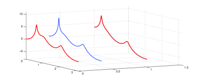
Refer to caption
Figure 3: logfτ,AR(θ)subscript𝑓𝜏AR𝜃\log f_{\tau,{\rm AR}}(\theta) for τ=13,23,43𝜏132343\tau=\frac{1}{3},\frac{2}{3},\frac{4}{3} (blue), τ=0,1𝜏01\tau=0,1 (red).

Likewise logfτ,linearsubscript𝑓𝜏linear\log f_{\tau,{\rm linear}} in Figure 4 breaks up for τ=43𝜏43\tau=\frac{4}{3}, since f43,linearsubscript𝑓43linearf_{\frac{4}{3},{\rm linear}} becomes negative for a range of frequencies –dashed curve indicates the absolute value of the logarithm when this takes complex values.
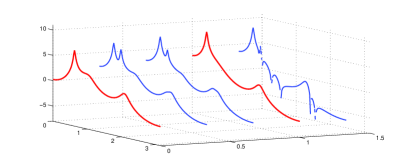
Refer to caption
Figure 4: logfτ,linear(θ)subscript𝑓𝜏linear𝜃\log f_{\tau,{\rm linear}}(\theta) for τ=13,23,43𝜏132343\tau=\frac{1}{3},\frac{2}{3},\frac{4}{3} (blue), τ=0,1𝜏01\tau=0,1 (red).

The plot of logfτ,geodesicsubscript𝑓𝜏geodesic\log f_{\tau,{\rm geodesic}} is defined for all the τ𝜏\tau and shown in Figure 5.

Refer to caption
Figure 5: logfτ,geodesic(θ)subscript𝑓𝜏geodesic𝜃\log f_{\tau,{\rm geodesic}}(\theta) for τ=13,23,43𝜏132343\tau=\frac{1}{3},\frac{2}{3},\frac{4}{3} (blue), τ=0,1𝜏01\tau=0,1 (red).

It is worth pointing out how two apparent “modes” in fτ,linearsubscript𝑓𝜏linearf_{\tau,{\rm linear}} and fτ,geodesicsubscript𝑓𝜏geodesicf_{\tau,{\rm geodesic}} are swapping their dominance, which does not occur when following fτ,ARsubscript𝑓𝜏ARf_{\tau,{\rm AR}}.

A multivariable example:

Consider the two matrix-valued power spectral densities

f0=[100.1ejθ1][1|a0(ejθ)|2001][10.1ejθ01]subscript𝑓0delimited-[]100.1superscript𝑒j𝜃1delimited-[]1superscriptsubscript𝑎0superscript𝑒j𝜃2001delimited-[]10.1superscript𝑒j𝜃01\displaystyle f_{0}=\left[\begin{array}[]{cc}1&0\\ 0.1e^{{\rm j}\theta}&1\\ \end{array}\right]\left[\begin{array}[]{cc}\frac{1}{|a_{0}(e^{{\rm j}\theta})|^{2}}&0\\ 0&1\\ \end{array}\right]\left[\begin{array}[]{cc}1&0.1e^{-{\rm j}\theta}\\ 0&1\\ \end{array}\right]
f1=[10.1ejθ01][1001|a1(ejθ)|2][100.1ejθ1].subscript𝑓1delimited-[]10.1superscript𝑒j𝜃01delimited-[]1001superscriptsubscript𝑎1superscript𝑒j𝜃2delimited-[]100.1superscript𝑒j𝜃1\displaystyle f_{1}=\left[\begin{array}[]{cc}1&0.1e^{{\rm j}\theta}\\ 0&1\\ \end{array}\right]\left[\begin{array}[]{cc}1&0\\ 0&\frac{1}{|a_{1}(e^{{\rm j}\theta})|^{2}}\\ \end{array}\right]\left[\begin{array}[]{cc}1&0\\ 0.1e^{-{\rm j}\theta}&1\\ \end{array}\right].

Typically, these reflect the dynamic relationship between two time series; in turn these may represent noise input/output of dynamical systems or measurements across independent array of sensors, etc. The particular example reflects the typical effect of an energy source shifting its signature from one of two sensors to the other as, for instance, a possible scatterer moves with respect to the two sensors.

Below f0subscript𝑓0f_{0} and f1subscript𝑓1f_{1} are shown in Fig. 6 and Fig. 7, respectively. Since the value of a power spectral density f𝑓f, at each point in frequency, is a Hermitian matrix, our convention is to show in the (1,1), (1,2) and (2,2) subplots the log-magnitude of the entries f(1,1),f(1,2)𝑓11𝑓12f(1,1),f(1,2) (which is the same as f(2,1)𝑓21f(2,1)) and f(2,2)𝑓22f(2,2), respectively. Then, since only f(1,2)𝑓12f(1,2) is complex (and the complex conjugate of f(2,1)𝑓21f(2,1)), we plot its phase in the (2,1) subplot.
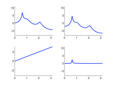
Refer to caption
Figure 6: Subplots (1,1), (1,2) and (2,2) show logf0(1,1),log|f0(1,2)|subscript𝑓011subscript𝑓012\log f_{0}(1,1),\log|f_{0}(1,2)| (same as log|f0(2,1)|subscript𝑓021\log|f_{0}(2,1)|) and logf0(2,2)subscript𝑓022\log f_{0}(2,2). Subplot (2,1) shows arg(f0(2,1))argsubscript𝑓021{\rm arg}(f_{0}(2,1)).
Refer to caption
Figure 7: Subplots (1,1), (1,2) and (2,2) show logf1(1,1),log|f1(1,2)|subscript𝑓111subscript𝑓112\log f_{1}(1,1),\log|f_{1}(1,2)| (same as log|f1(2,1)|subscript𝑓121\log|f_{1}(2,1)|) and logf0(2,2)subscript𝑓022\log f_{0}(2,2). Subplot (2,1) shows arg(f1(2,1))argsubscript𝑓121{\rm arg}(f_{1}(2,1)).

Three dimensional surface show the geodesic connecting f0subscript𝑓0f_{0} to f1subscript𝑓1f_{1} in Figure 8. Here, fτ,geodesicsubscript𝑓𝜏geodesicf_{\tau,{\rm geodesic}} is drawn using

fτ,geodesic=f012(f012f1f012)τf012.subscript𝑓𝜏geodesicsuperscriptsubscript𝑓012superscriptsuperscriptsubscript𝑓012subscript𝑓1superscriptsubscript𝑓012𝜏superscriptsubscript𝑓012\displaystyle f_{\tau,{\rm geodesic}}=f_{0}^{\frac{1}{2}}(f_{0}^{-\frac{1}{2}}f_{1}f_{0}^{-\frac{1}{2}})^{\tau}f_{0}^{\frac{1}{2}}.
Refer to caption
Figure 8: Subplots (1,1), (1,2) and (2,2) show logfτ(1,1),log|fτ(1,2)|subscript𝑓𝜏11subscript𝑓𝜏12\log f_{\tau}(1,1),\log|f_{\tau}(1,2)| (same as log|fτ(2,1)|subscript𝑓𝜏21\log|f_{\tau}(2,1)|) and logfτ(2,2)subscript𝑓𝜏22\log f_{\tau}(2,2). Subplot (2,1) shows arg(fτ(2,1))argsubscript𝑓𝜏21{\rm arg}(f_{\tau}(2,1)), for τ[0,1]𝜏01\tau\in[0,1].

It is interesting to observe the smooth shift of the energy across frequency and directionality.

VIII Conclusions

The aim of this study has been to develop multivariable divergence measures and metrics for matrix-valued power spectral densities. These are expected to be useful in quantifying uncertainty in the spectral domain, detecting events in non-stationary time series, smoothing and spectral estimation in the context of vector valued stochastic processes. The spirit of the work follows closely classical accounts going back to [1, 2] and proceeds along the lines of [7]. Early work in signal analysis and system identification has apparently focused only on divergence measures between scalar spectral densities, and only recently have such issues on multivariable power spectra attracted attention [8, 9]. Further, this early work on scalar power spectra was shown to have deep roots in statistical inference, the Fisher-Rao metric, and Kullback-Leibler divergence [6], [2, page 371], [7], [13]. Thus, it is expected that interesting connections between the geometry of multivariable power spectra and information geometry will be established as well.

References

  • [1] M. Basseville, “Distance measures for signal processing and pattern recognition,” Signal processing, vol. 18, no. 4, pp. 349–369, 1989.
  • [2] R. Gray, A. Buzo, A. Gray Jr, and Y. Matsuyama, “Distortion measures for speech processing,” Acoustics, Speech and Signal Processing, IEEE Transactions on, vol. 28, no. 4, pp. 367–376, 1980.
  • [3] C. Rao, “Information and the accuracy attainable in the estimation of statistical parameters,” Bull. Calcutta Math. Soc., vol. 37, pp. 81–91, 1945.
  • [4] S.-I. Amari and H. Nagaoka, Methods of information geometry.   Amer. Math. Soc., 2000.
  • [5] N. Cencov, Statistical decision rules and optimal inference.   Amer. Math. Soc., 1982, no. 53.
  • [6] R. Kass and P. Vos, Geometrical foundations of asymptotic inference.   Wiley New York, 1997.
  • [7] T. Georgiou, “Distance and Riemannian metrics for spectral density functions,” Signal Processing, IEEE Transactions on, vol. 55(8), pp. 3995–4003, 2007.
  • [8] A. Ferrante, C. Masiero, and M. Pavon, “Time and spectral domain relative entropy: A new approach to multivariate spectral estimation,” Arxiv preprint arXiv:1103.5602, 2011.
  • [9] A. Ferrante, M. Pavon, and F. Ramponi, “Hellinger versus Kullback–Leibler multivariable spectrum approximation,” Automatic Control, IEEE Transactions on, vol. 53, no. 4, pp. 954–967, 2008.
  • [10] T. Georgiou, “Relative entropy and the multivariable multidimensional moment problem,” Information Theory, IEEE Transactions on, vol. 52, no. 3, pp. 1052–1066, 2006.
  • [11] R. Bhatia, Positive definite matrices.   Princeton Univ Pr, 2007.
  • [12] M. Pinsker, Information and information stability of random variables and processes.   Izv. Akad. Nauk. SSSR, Moscow, 1960, English translation: San Francisco,CA: Holden-Day, 1964.
  • [13] S. Yu and P. Mehta, “The Kullback–Leibler rate pseudo-metric for comparing dynamical systems,” Automatic Control, IEEE Transactions on, vol. 55, no. 7, pp. 1585–1598, 2010.
  • [14] N. Wiener and P. Masani, “The prediction theory of multivariate stochastic processes, Part I,” Acta Math., vol. 98, pp. 111–150, 1957.
  • [15] P. Masani, Recent trends in multivariable prediction theory. (Krishnaiah, P.R., Editor), Multivariate Analysis, pp. 351-382.   Academic Press, 1966.
  • [16] T. Georgiou, “The Carathéodory–Fejér–Pisarenko decomposition and its multivariable counterpart,” Automatic Control, IEEE Transactions on, vol. 52, no. 2, pp. 212–228, 2007.
  • [17] P. Petersen, Riemannian geometry.   Springer Verlag, 2006.
  • [18] J. Jost, Nonpositive curvature: geometric and analytic aspects.   Birkhäuser, 1997.
  • [19] M. Moakher, “A differential geometric approach to the geometric mean of symmetric positive-definite matrices,” SIAM Journal on Matrix Analysis and Applications, vol. 26, no. 3, pp. 735–747, 2005.
  • [20] A. Kolmogorov and S. Fomin, Elements of the theory of functions and functional analysis, Volume 2.   Graylock Press, 1961.
  • [21] R. Horn and C. Johnson, Topics in matrix analysis.   Cambridge university press, 1994.
  • [22] ——, Matrix analysis.   Cambridge university press, 2005.