Non-radial modes in cool stars

Abstract

In cool stars that oscillate like the Sun, non-radial modes become mixed as the stars evolve. The mixing is caused by the coupling between g-modes in the stellar core and p-modes in the envelope, which results in distinctly different and more complex frequency spectra for subgiants and red giants than seen in main sequence stars. Using a new version of the ‘scaled’ échelle diagram, I illustrate how the frequencies of non-radial modes evolve during the evolution from the main sequence to the red giant branch, and I show how they depend on stellar mass and metallicity. Then, with focus on the dipole ($l=1$) modes, which show the strongest effects from mixing, I present a toy model to fit, and hence identify, those modes in a large series red giant models.

1 Introduction

Stellar models predict that non-radial oscillation modes in stars like the Sun will become of a mixed character as the stars evolve off the main sequence (Osaki 1975). The mixing, which is caused by the coupling of two modes (a g-mode in the stellar core and a p-mode in the envelope) will result in shifts of the mode frequencies - known as mode bumping - as the two modes undergo so-called avoided crossings. As a result, mixed modes do not follow the usual asymptotic relation of regular spaced high radial order p-mode frequencies, $\nu$, as expressed by (e.g.  Vandakurov 1968; Tassoul 1980; Christensen-Dalsgaard 2011)

$$\nu_{nl}=\Delta\nu(n+l/2+\epsilon)-\delta\nu_{0l}$$ (1)

where the small frequency separation

$$\delta\nu_{0l}\propto(l+1/2)^{2}\frac{\Delta\nu}{\nu_{nl}}\,.$$ (2)

Here $n$ is the radial order, $l$ is the degree, $\epsilon$ is a dimensionless offset, and $\Delta\nu$ is the separation between over tone modes of the same degree. When visualized in the échelle diagram, where we plot mode frequency versus the frequency modulo the large frequency separation, $\Delta\nu$, mixed modes can show strong departures from the almost vertical ridges of the non-mixed modes, which I will discuss next.

2 The scaled échelle diagram

A useful diagram to compare mode frequencies of many stars (or models) is the scaled échelle diagram introduced by Bedding & Kjeldsen (2010). Their Method 2 sought to make the ridges of the radial modes coincide for different, though still similar, stars by fine tuning $\Delta\nu$; in essence removing any differences in $\epsilon$ by allowing the ridges to depart slightly from vertical. This provides a clear picture of how the modes of different degree are positioned relative to one another in a comparative analysis. Here I will use a slightly modified version of this method to show the evolution of a large series of models ranging from the main sequence to the red giant branch (RGB). For each model, $\Delta\nu$ is derived from the four radial modes closest to the frequency of maximum power, $\nu_{\mathrm{max}}$ (scaled from the solar value according to Kjeldsen & Bedding (1995)), and the variation in $\epsilon$ from one model to the next is removed by shifting the frequencies to a common value of $\epsilon=1.2$; hence maintaining strictly vertical ridges of the radial modes. This could therefore be appropriately called a shifted échelle diagram.

The stellar models were derived with ASTEC (Christensen-Dalsgaard 2008a) and adiabatic frequencies were calculated using the ADIPLS code (Christensen-Dalsgaard 2008b). The models range in mass from 0.8$M_{\odot}$, to 1.6$M_{\odot}$ in steps of 0.2$M_{\odot}$, and in $Z$ from 0.011 to 0.028 in steps of 0.1 dex in $\log Z/X$ (with $X=0.7$ fixed). The tracks were evolved from the zero-age-main-sequence (ZAMS) towards, but not quite reaching, the tip of the RGB. Details on the model physics, can be found in Stello et al. (2009) and references therein. The tracks for $Z=0.017$ (approximately solar metallicity) are shown in Figure 1, where I have used $\nu_{\mathrm{max}}$  as the proxy for luminosity to make it more useful in comparison with the following figures.

Figure 1.: Asteroseismic Hertzsprung-Russell diagram with $\nu_{\mathrm{max}}$ as luminosity proxy. Tracks are for $Z=0.017$ and their masses in solar units are shown at the ZAMS.

Figure 2.: Échelle diagram for series of models along a 1.0M_⊙ track ($Z=0.017$, [Fe/H$]\simeq 0.0$; see Figure 1). For each model the four modes closest to $\nu_{\mathrm{max}}$ are plotted after they were shifted to a common value of $\epsilon=1.2$. The dotted line shows the halfway point between adjacent radial modes.

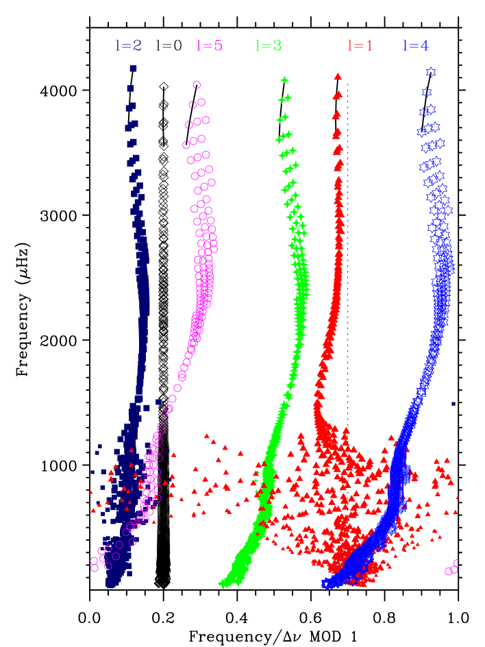
In Figure 2, I show an échelle diagram for a series of models along the one solar mass track, where four orders are plotted for each model. The symbol sizes are scaled according to the reciprocal of the square root of the mode inertia, normalized to the radial modes, but set to zero below a certain threshold for clarity. Several features are apparent in this diagram.

1. We see an increasing tilt of the non-radial ridges with increasing $l$. To illustrate this, I have connected modes of the same degree by lines for the ZAMS model. The tilt can be explained by the last term in the asymptotic relation, $\delta\nu_{0l}$ (Eq. 2), where a higher $l$ implies a higher frequency dependence, and hence a stronger tilt.

2. The position of the non-radial ridges, and hence the small separations, changes quite significantly with evolution. After moderate changes during the main sequence, there seems to be a slight pause during the subgiant phase where the stellar density is not changing by much, before more dramatic changes occur during the ascent of the RGB. That the change is larger for increasing mode degree is explained by the same asymptotic term as for the above tilt. Interestingly, this evolution of the ridge positions shows some similarities to the variation seen in $\epsilon$ as a function of $\nu_{\mathrm{max}}$ (White et al. 2011).

3. At a certain point during the evolution, corresponding roughly to the transition between the main sequence and the subgiant phase, mixed modes start to appear, most clearly for $l=1$ and $l=2$, leading to modes spreading across the entire echelle diagram ($l=1$ in particular).

4. After the subgiant phase the mixed modes become more confined as the models evolve up the RGB. Ultimately, near the tip of the RGB, the coupling between p- and g-modes become so weak (efficient mode trapping) that we expect to see only one mode per degree per radial order, as in the main sequence phase (Dupret et al. 2009).

5. As first observed by Bedding et al. (2010) and shown for stellar models by Montalbán et al. (2010), the small separation, $\delta\nu_{10}$, between the the $l=1$ modes and the point halfway between consecutive radial modes (dotted line) becomes negative for the red giant models.

Note that the less dense $l=5$ ridge arise simply because these modes were not derived for all models along the evolution track at the subgiant and red giant phases.

2.1 Changing mass and metallicity

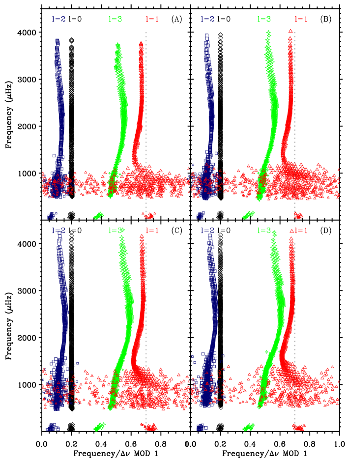
To illustrate how the different features seen in the échelle diagram depend on stellar mass and metallicity, I show examples for $l\leqq 3$ of models with a range of masses and metallicities (Figures 3, 4). Due to the high computational requirements for deriving mode frequencies of evolved stellar models there is a lack of frequencies in the model grid, which appears near the base of the RGB (300$\mu$Hz $\lesssim$ $\nu_{\mathrm{max}}$ $\lesssim 500$$\mu$Hz). Fortunately, the highly evolved red giant models at even lower $\nu_{\mathrm{max}}$ enables ’interpolation by eye’ to bridge the gap.

Figure 3.: Échelle diagram for series of models along the A: 0.8M_⊙, B: 1.2M_⊙, C: 1.4M_⊙, and D: 1.6M_⊙ tracks ($Z=0.017$, see Figure 1). The y-axes are rescaled for the lower panels for improved visibility.

Figure 4.: Échelle diagram for series of models along 1.0M_⊙ tracks of A: $Z=0.011$ ([Fe/H$]\simeq-0.19$), B: $Z=0.014$ ([Fe/H$]\simeq-0.08$), C: $Z=0.022$ ([Fe/H$]\simeq 0.11$), and D: $Z=0.028$ ([Fe/H$]\simeq 0.22$).

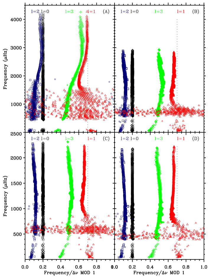
It is evident from Figure 3 that the ridge positions change significantly as a function of mass, with lower masses showing smaller separations between the odd ridges ($\delta\nu_{02}$) and even ridges ($\delta\nu_{13}$), respectively. The higher mass models, which exhibit the smallest density changes during the subgiant phase, show more static ridge positions during this phase in agreement with Eq. 2 and the observation made in Figure 2 (point 2). We further see a hint that the $l=2$ modes spread out more for the least massive models, indicative of stronger mode coupling.

If we turn our attention to the effect from metallicity (Figure 4), we see that an increase in $Z$ results in a decrease in the separations between the odd ridges and even ridges, respectively. This is in qualitative agreement with the effect we saw on mass, namely that the cooler the model the smaller the separations $\delta\nu_{02}$ and $\delta\nu_{13}$ become.

2.2 Mixed dipole modes in red giants

In the following I will focus on the lower part of Figure 2 where we see increased complexity in the $l=1$ ridge due to mode mixing. In particular I will address how to identify the $l=1$ modes in frequency spectra of red giants.

The complicated frequency spectra of $l=1$ modes in subgiants can in many cases be successfully fitted, resulting in correct identification of the mode degree (Deheuvels & Michel 2010, Benomar et al. in prep.). However, can something similar be done for red giant stars? To motivate this question, I show the frequency spectra of two red giants in Figure 5.

Figure 5.: Frequency spectra of an RGB star and a red clump star (taken from Bedding et al. 2011). Mode degree is indicated.

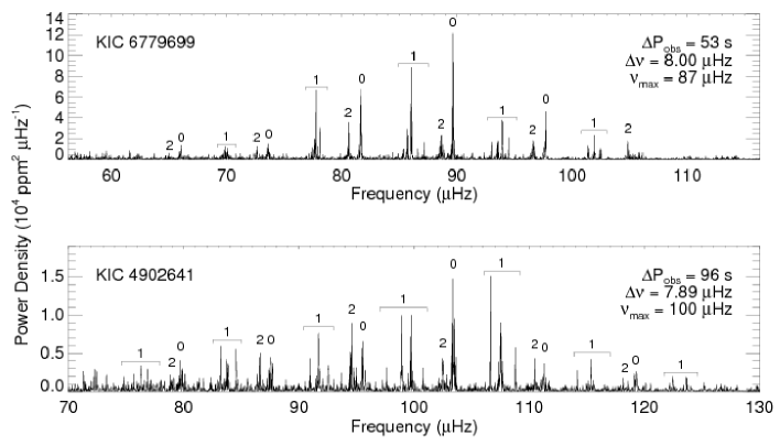
The weaker mode coupling in red giants imply we do not see the $l=1$ modes appear everywhere, as in subgiants (Figure 2), but rather within well confined clusters, one for each radial order (centered at the frequency of the ’unperturbed’ p-mode in the hypothetical case where there would be no coupling with the g-modes in the core). On the one hand, this makes the spectra more simple as we avoid a very dense spectrum of $l=1$ modes that overlaps with all the other modes. On the other hand, the slightly complicated frequency separations of these modes (Beck et al. 2011; Bedding et al. 2011) makes it difficult to estimate how many modes are in fact ’missing in the gaps’ between each cluster of modes, and hence hinders a straightforward determination of the frequencies of the undetected modes. In practise this means that it can become difficult to make judgment on whether a peak in the observed frequency spectrum belongs to the sequences of $l=1$ modes or whether it is due to a mode of a different degree, or simply noise.

Fortunately, for stellar models we have frequencies for all modes available, even those in the gaps that are not detectable in reality. This can help us develop ways to analyse the complex frequency spectra observed in red giants. As a first step towards fitting observed $l=1$ modes I will show some preliminary results for what one obtains when fitting a simple toy model to the stellar model frequencies. The aim of this exercises is to identify relations between on the one hand the parameters that describe the toy model and one the other hand the quantities that we are able to detect in the observed frequency spectra – ultimately enabling us to make informed decisions and on how to interpret the observations.

Figure 6.: Period spacing versus frequency for dipole modes (diamonds) of Model A, which has $T_{\mathrm{eff}}$ $=4745\,$K and $L/\mathrm{L}_{\odot}=56$ (marked in Figure 7b). Toy model fit is shown by thick solid blue line. Resulting fitting parameters, $\Delta P_{g}$, FWHM, and Depth are indicated (see text for details).

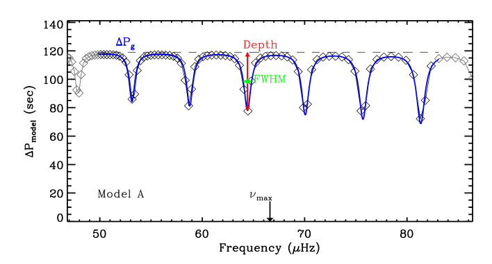
Figure 6 shows the period spacing of the $l=1$ modes from a model located on the RGB. The period spacing is approximately constant as expected from asymptotic theory of pure g-modes (e.g.  Christensen-Dalsgaard 2011, and references therein). The departure from the constant spacing, seen as regular dips, are caused by the coupling between the g- and p-modes, which shifts the frequencies. The dips are separated by $\Delta\nu$ – the separation between the unperturbed p-modes. The most weakly coupled modes are almost pure g-modes, hence showing near equal period spacings. However, being pure g-mode means they are basically contained in the core, and hence not observable. The more strongly coupled modes, which show the largest departure from equal period spacing, are more p-mode like, and have therefore significant amplitudes at the surface and are the ones we detect as small clusters.

Figure 7.: (a) Evolution track of 2.4M_⊙ track. (b)-(d) Results of fitting the toy model (Figure 6 thick blue curve) to each model along the track. Plotted values of FWHM and Depth are evaluated at $\nu_{\mathrm{max}}$.

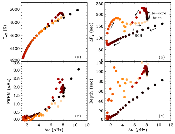
I have simultaneously fitted a series of Lorentzian profiles, one for each dip to a series of stellar model frequencies of dipole modes. The free parameters in the fit are $\Delta P_{g}$ (the true g-mode spacing unperturbed by mixing with p-modes), FWHM (the width of the Lorentzian), $\delta$(FWHM)/$\delta f$ (the change in the width as a function of frequency), Depth (the depth of the dip), $\delta$(Depth)/$\delta f$ (the change in the depth as a function of frequency), and the frequency of the centre of each Lorentzian profile, assumed to be strictly equally spaced. Figure 7a shows a 2.4M_⊙ track evolving from the base of the RGB to the base of the asymptotic giant branch (like a transposed Hertzsprung Russell diagram), and Figures 7b-d show the result of fitting the toy model to the stellar models along that track. An example of a fit is shown by the blue curve in Figure 6. Interestingly, there seems to be a strong relation between $\Delta P_{g}$ and Depth, but Depth is not simply $\frac{1}{2}\Delta P_{g}$ as suggested by Bedding et al. (2011). Although FWHM and Depth are both related to the coupling strength between the g- and p-modes, only Depth separates the RGB from the red clump, while FWHM is largely a function of $T_{\mathrm{eff}}$. When repeated for stellar models of different masses, the relations between the toy model parameters and the seismic observables change. Quantifying these relations will help create a formalism to fit mixed mode frequencies from observations.

3 Summary and future work

I have shown that a new version of the ‘scaled’ échelle diagram can be useful to compare an ensemble of stellar models, and in particular to show the evolution of pulsation frequencies from the main sequence to the RGB as well as how the frequencies depend on mass and metallicity. For red giants we see that the $l=1$ modes become more confined as small clusters of modes. While this in some sense makes the frequency spectra simpler, it also brings new challenges by making it harder to determine the frequencies of all the modes between each cluster. I briefly demonstrated that fitting a simple toy model to stellar model frequencies can aid in establishing relations between seismic observables and the toy model parameters. When fully developed this could lead to a robust way to fit the observed $l=1$ frequencies and hence to determine the characteristics of their complex frequency separations.

Acknowledgments

I would like to thank Hiromoto Shibahashi for support to attend this conference, and all participants who despite the unusual circumstances took this as an experience…Kampai!. I would also like to thank Jørgen Christensen-Dalsgaard for comments on manuscript.

References

- Beck et al. (2011) Beck, P. G., Bedding, T. R., Mosser, B., Stello, D., Garcia, R. A., Kallinger, T., Hekker, S., Elsworth, Y., Frandsen, S., Carrier, F., De Ridder, J., Aerts, C., White, T. R., Huber, D., Dupret, M., Montalbán, J., Miglio, A., Noels, A., Chaplin, W. J., Kjeldsen, H., Christensen-Dalsgaard, J., Gilliland, R. L., Brown, T. M., Kawaler, S. D., Mathur, S., & Jenkins, J. M. 2011, Science, 332, 205
- Bedding et al. (2010) Bedding, T. R., Huber, D., Stello, D., Elsworth, Y. P., Hekker, S., Kallinger, T., Mathur, S., Mosser, B., Preston, H. L., Ballot, J., Barban, C., Broomhall, A. M., Buzasi, D. L., Chaplin, W. J., García, R. A., Gruberbauer, M., Hale, S. J., De Ridder, J., Frandsen, S., Borucki, W. J., Brown, T., Christensen-Dalsgaard, J., Gilliland, R. L., Jenkins, J. M., Kjeldsen, H., Koch, D., Belkacem, K., Bildsten, L., Bruntt, H., Campante, T. L., Deheuvels, S., Derekas, A., Dupret, M., Goupil, M., Hatzes, A., Houdek, G., Ireland, M. J., Jiang, C., Karoff, C., Kiss, L. L., Lebreton, Y., Miglio, A., Montalbán, J., Noels, A., Roxburgh, I. W., Sangaralingam, V., Stevens, I. R., Suran, M. D., Tarrant, N. J., & Weiss, A. 2010, ApJ, 713, L176. 1001.0229
- Bedding & Kjeldsen (2010) Bedding, T. R., & Kjeldsen, H. 2010, Communications in Asteroseismology, 161, 3. 1001.5038
- Bedding et al. (2011) Bedding, T. R., Mosser, B., Huber, D., Montalbán, J., Beck, P., Christensen-Dalsgaard, J., Elsworth, Y. P., García, R. A., Miglio, A., Stello, D., White, T. R., De Ridder, J., Hekker, S., Aerts, C., Barban, C., Belkacem, K., Broomhall, A., Brown, T. M., Buzasi, D. L., Carrier, F., Chaplin, W. J., di Mauro, M. P., Dupret, M., Frandsen, S., Gilliland, R. L., Goupil, M., Jenkins, J. M., Kallinger, T., Kawaler, S., Kjeldsen, H., Mathur, S., Noels, A., Aguirre, V. S., & Ventura, P. 2011, Nat, 471, 608. 1103.5805
- Christensen-Dalsgaard (2008a) — 2008a, Ap&SS, 316, 13. 0710.3114
- Christensen-Dalsgaard (2008b) Christensen-Dalsgaard, J. 2008b, Ap&SS, 316, 113. 0710.3106
- Christensen-Dalsgaard (2011) — 2011, ArXiv e-prints. 1106.5946
- Deheuvels & Michel (2010) Deheuvels, S., & Michel, E. 2010, Ap&SS, 328, 259. 0912.2834
- Dupret et al. (2009) Dupret, M., Belkacem, K., Samadi, R., Montalban, J., Moreira, O., Miglio, A., Godart, M., Ventura, P., Ludwig, H., Grigahcène, A., Goupil, M., Noels, A., & Caffau, E. 2009, A&A, 506, 57. 0906.3951
- Kjeldsen & Bedding (1995) Kjeldsen, H., & Bedding, T. R. 1995, A&A, 293, 87. URL http://adsabs.harvard.edu/cgi-bin/nph-bib_query?bibcode=1995%A%26A...293...87K&db_key=AST
- Montalbán et al. (2010) Montalbán, J., Miglio, A., Noels, A., Scuflaire, R., & Ventura, P. 2010, ApJ, 721, L182. 1009.1754
- Osaki (1975) Osaki, J. 1975, PASJ, 27, 237
- Stello et al. (2009) Stello, D., Chaplin, W. J., Bruntt, H., Creevey, O. L., García-Hernández, A., Monteiro, M. J. P. F. G., Moya, A., Quirion, P.-O., Sousa, S. G., Suárez, J.-C., Appourchaux, T., Arentoft, T., Ballot, J., Bedding, T. R., Christensen-Dalsgaard, J., Elsworth, Y., Fletcher, S. T., García, R. A., Houdek, G., Jiménez-Reyes, S. J., Kjeldsen, H., New, R., Régulo, C., Salabert, D., & Toutain, T. 2009, ApJ, 700, 1589. 0906.0766
- Tassoul (1980) Tassoul, M. 1980, ApJS, 43, 469. URL http://adsabs.harvard.edu/cgi-bin/nph-bib_query?bibcode=1980A%pJS...43..469T&db_key=AST
- Vandakurov (1968) Vandakurov, Y. V. 1968, Soviet Astronomy, 11, 630
- White et al. (2011) White et al. 2011. ApJ submitted