Geometry of Complex Networks and Topological Centrality

Abstract

We explore the geometry of complex networks in terms of an n-dimensional Euclidean embedding represented by the Moore-Penrose pseudo-inverse of the graph Laplacian $(\mathbf{L}^{+})$. The squared distance of a node $i$ to the origin in this n-dimensional space $(l^{+}_{ii})$, yields a topological centrality index, defined as $\mathcal{C}^{*}(i)=1/l^{+}_{ii}$. In turn, the sum of reciprocals of individual node centralities, $\sum_{i}1/\mathcal{C}^{*}(i)=\sum_{i}l^{+}_{ii}$, or the trace of $\mathbf{L}^{+}$, yields the well-known Kirchhoff index $(\mathcal{K})$, an overall structural descriptor for the network. To put in context this geometric definition of centrality, we provide alternative interpretations of the proposed indices that connect them to meaningful topological characteristics — first, as forced detour overheads and frequency of recurrences in random walks that has an interesting analogy to voltage distributions in the equivalent electrical network; and then as the average connectedness of $i$ in all the bi-partitions of the graph. These interpretations respectively help establish the topological centrality $(\mathcal{C}^{*}(i))$ of node $i$ as a measure of its overall position as well as its overall connectedness in the network; thus reflecting the robustness of $i$ to random multiple edge failures. Through empirical evaluations using synthetic and real world networks, we demonstrate how the topological centrality is better able to distinguish nodes in terms of their structural roles in the network and, along with Kirchhoff index, is appropriately sensitive to perturbations/rewirings in the network.

1 Introduction

Unlike traditional studies on network robustness, that typically treat networks as combinatoric objects and rely primarily on classical graph-theoretic concepts (such as degree distributions, geodesics and minimum cuts), we explore a geometric approach as an alternative. To do so, we embed the network into an $n$-dimensional Euclidean space ($n$ being the number of nodes in the network) represented by the Moore-Penrose pseudo-inverse of its graph Laplacian, denoted henceforth by $\mathbf{L}^{+}$. The diagonal entries of $\mathbf{L}^{+}$, denoted as $l^{+}_{ii}$ for the node $i$, represent the squared distance of node $i$ to the origin in this $n-dimensional$ space and provide a measure of the node’s topological centrality, given as $\mathcal{C}^{*}(i)=1/l^{+}_{ii}$. Closer the node $i$ is to the origin in this space, or equivalently lower the $l^{+}_{ii}$, more topologically central $i$ is. Similarly, the trace of $\mathbf{L}^{+}$, $Tr(\mathbf{L}^{+})=\sum_{i}1/\mathcal{C}^{*}(i)$, determines the overall volume of the embedding and yields the well-known Kirchhoff index $(\mathcal{K})$, a structural descriptor for the network as a whole. Once again, lower the value of $\mathcal{K}$ for a network (from amongst all possible networks with the same number of nodes and edges), more compact the embedding, and more structurally robust the overall network is. In short, topological centrality defines a ranking of the nodes of a given network, where as the Kirchhoff index provides a geometric measure to rank different networks of comparable sizes.

In order to illustrate how the two geometric quantities defined above actually reflect the structural properties of the underlying network, and in particular to structural robustness against multiple failures, we provide three alternative interpretations for them in terms of: (a) detour overheads in random walks, (b) voltage distributions and the phenomenon of recurrence when the network is treated as an electrical circuit, and (c) the average connectedness of nodes when the network breaks into two, thereby making global communication untenable. We describe each of these in detail below.

First, we show how topological centrality of a node reveals its overall position in the network. By equating topological centrality of a node $i$, i.e. $\mathcal{C}^{*}(i)=1/l^{+}_{ii}$, to the (reciprocal of) average detour overhead incurred when a random walk between any source destination pair is forced to go through $i$, we get a measure of the node’s position. Intuitively, the average overhead incurred in such forced detours (measured in terms of the number of steps in the random walk) is lower if node $i$ is centrally positioned in the network (higher $\mathcal{C}^{*}(i)$ and lower $l^{+}_{ii}$) and higher if $i$ is peripheral. Secondly, we show how $\mathcal{C}^{*}(i)$ captures voltage distribution when the network is transformed into an equivalent electrical network (EEN). This, in turn, is related to the probability with which a random detour through $i$ returns to the source node; referred to as the phenomenon of recurrence in random walk literature. To be precise, higher $\mathcal{C}^{*}(i)$ implies that a random detour through node $i$ forces the random walk between any source destination pair to return to the source node with lower probability, thereby incurring lower detour overhead. Both of these interpretations, namely average detour overhead and probability of recurrence, therefore, demonstrate how $\mathcal{C}^{*}(i)$ quantifies the overall position of node $i$ in the network. Finally, we establish how $\mathcal{C}^{*}(i)$ captures the overall connectedness of node $i$. To do so, we equate it to the number of nodes that $i$ can communicate with when a sub-set of edges in the network fail in such a way that the network is partitioned into two connected sub-networks. As connected bi-partitions represent a regressed state of the network when not all pairs of nodes can maintain communication, a higher value of $\mathcal{C}^{*}(i)$, implies that $i$ is present in the larger of the two sub-networks, on an average, in such bi-partitions. Thus, $\mathcal{C}^{*}(i)$ reflects the immunity/vulnerability of node $i$ towards multiple edge failures in the network, a distinct topological characteristic.

Through numerical simulations using synthetic and realistic network topologies, we demonstrate that our new indices better characterize robustness of nodes in network, both in terms of position as well as connectedness, as compared to other existing metrics (e.g. node centrality measured based on degree, shortest paths, etc.). A rank-order of nodes by their topological centralities $(\mathcal{C}^{*}(i))$ helps distinguish them in terms of their structural roles (such as core, gateway, etc.). Also, topological centrality and Kirchhoff index, are both appropriately sensitive to local perturbations in the network, a desirable property not displayed by some of the other popular centrality indices in literature (as shown later in this paper).

The rest of the paper is organized as follows: we begin by providing a brief overview of several structural indices, characterizing node centrality as well as overall descriptors for networks, found in literature in §2. §3 introduces a geometric embedding of the network using the eigen-space of $\mathbf{L}^{+}$, topological centrality and Kirchhoff index as measures of robustness. §4 demonstrates how topological centrality of a node reflects the average detour overhead in random walks through a particular node in question followed by its equivalence to the probability of recurrence. In §5 we show how topological centrality captures the average connectedness of nodes in the bi-partitions of a network. §6 presents comparative empirical analysis with simulated as well as real world networks while in §7 we analyze the computational complexity of the proposed metrics with respect to others popular in literature. Finally, the paper is concluded with a discussion of future work in §8.

2 Related Work

Robustness of nodes to failures in complex networks is dependent on their overall position and connectedness in the network. Several centralities, that characterize position and/or connectedness of nodes in complex networks in different ways, have therefore been proposed in literature. Perhaps the simplest of all is degree — the number of edges incident on a node. Degree is essentially a local measure i.e. a first oder/one-hop connectedness index. A second-order variant called joint-degree, given by the product of degrees of a pair of nodes that are connected by an edge in the network, is also in vogue. However, except in scale free networks that display the so called rich club connectivity [2, 15, 16], neither degree nor joint-degree determine the overall position or the connectedness of nodes.

A class of structural indices called betweennesses, namely shortest path/geodesic $(GB)$ [20, 21], flow $(FB)$ [22] and random-walk $(RB)$ [30] betweenness respectively quantify the positions of nodes, with respect to source destination pairs in the network. The set of betweennesses, therefore, reflect the role played by a node in the communication between other node-pairs in the network and are not the measures of a node’s own connectedness.

Another popular centrality measure is geodesic closeness $(GC)$[20, 21]. It is defined as the (reciprocal of) average shortest-path distance of a node from all other nodes in the network. Clearly, geodesic closeness is a $p^{th}$-order measure of connectedness where $p=\{1,2,...,\delta\}$, $\delta$ being the geodesic diameter of the graph, and is better suited for characterizing global connectedness properties than the aforementioned indices. However, communication in networks is not always confined to shortest paths alone and $GC$ being geodesic based, ignores other alternative paths between nodes, however competitive they might be, and thus only partially captures connectedness of nodes. Some all paths based counterparts of geodesic closeness include information centrality [38] and random-walk centrality [32], that use random-walk based approach to measure centrality. In [7], several centrality measures based on network flow, and collectively referred to as structural centrality, have also been discussed in great detail.

Recently, subgraph centrality $(SC)$ — the number of subgraphs of a graph that a node participates in — has also been proposed [14]. In principle, a node with high subgraph centrality, should be better connected to other nodes in the network through redundant paths. Alas, subgraph centrality is computationally intractable and the proposed index in [14] approximates subgraph centrality by the sum of lengths of all closed walks, weighed in inverse proportions by the factorial of their lengths. This inevitably results in greater correlation with node degrees as each edge contributes to closed random-walks of lengths $2,4,6,...$ and thus introduces local connectivity bias. In a subsequent paper, Estrada et al introduce the concept of vibrations to measure node vulnerability in complex networks [13]. Their index called node displacement bears significant resemblance to information centrality and has interesting analogies to physical systems. However, once again the true topological significance of the centrality measure, in terms of connectedness is wanting.

Our aim in this work, therefore, is to provide an index for robustness of nodes in complex networks, that effectively reflects both the position and connectedness properties of nodes and consequently, by extension, of the overall network.

3 Geometric Embedding of Networks using $\mathbf{L}^{+}$, Topological Centrality and Kirchhoff Index

In studying the geometry of networks, we first need to embed a network, represented abstractly as a graph, into an appropriate space endowed with a metric function (mathematically, a metric space). In this section, we first describe just such a metric space in terms of the the Moore-Penrose pseudo-inverse of the combinatorial Laplacian (§3.1). Next, using the geometric attributes of this metric space, we define the topological centralities for individual nodes as well as the Kirchhoff index for the network as a whole (§3.2).

3.1 Network as a Graph, the Laplacian and a Euclidean Embedding

Given a complex network, we represent its topology as a weighted undirected graph, $G=(V,E,W)$, where $V(G)$ is the set of nodes; $E(G)$ the set of edges; and $W=\{w_{uv}\in\Re^{+}:e_{uv}\in E(G)\}$ is a set of weights assigned to each edge of the graph (here $\Re^{+}$ denotes the set of nonnegative real numbers). These weights can be used to represent a variety of affinity/distance measures, depending upon the context, such as latency or capacity in traditional communication networks, as well as friendship and acquaintance type relationships in the social counterparts. We define $\mathbf{A}=[a_{ij}]$ as the affinity matrix of $G(V,E,W)$, such that $a_{ij}=w_{ij}$ represents the affinity between nodes $i$ and $j$: larger the value of $a_{ij}$ is, closer the nodes $i$ and $j$ are. For a simple graph where $w_{ij}\in\{0,1\}$, $\mathbf{A}$ is simply the standard adjacency matrix of the graph $G$. Let $n=|V(G)|$ be the number of nodes in $G$ (also called the order of G). For $1\leq i\leq n$, we define $d(i)=\sum_{j}a_{ij}$, which is the (generalized) degree of node $i$. The sum of node degrees is often referred to as the volume of the graph, given as $Vol(G)=\sum_{i\in V(G)}d(i)$. It is easy to see that when the graph is unweighted, $Vol(G)=2|E(G)|$.

The combinatorial Laplacian of the graph $G(V,E,W)$, is defined as $\mathbf{L}=\mathbf{D}-\mathbf{A}$, where $\mathbf{D}=[d_{ii}]=d(i)$ is a diagonal matrix with the node degrees on the diagonal. $\mathbf{L}$ is a square, symmetric, doubly-centered (all rows and columns sum up to 0) and positive semidefinite matrix [3] with $n$ non-negative eigen values. By convention, we order the eigen values of $\mathbf{L}$ in decreasing order of magnitude as $[\lambda_{1}\geq\lambda_{2}\geq...\lambda_{n-1}>\lambda_{n}=0]$. Similarly for $1\leq i\leq n$, let $\mathbf{u}_{i}$ be the corresponding eigenvector of $\lambda_{i}$. If the network is connected (which we assume to be the case henceforth), the smallest eigen value $\lambda_{n}=0$ and its corresponding eigen vector $\mathbf{u}_{n}=[1,1,...,1]$ are both unique. Also, the eigen vectors of $\mathbf{L}$ are mutually perpendicular, i.e. $\mathbf{u}_{i}\cdot\mathbf{u}_{j}=0,\forall i,j$ (where $(\cdot)$ is the inner product). Therefore, the matrix of eigen vectors $\mathbf{U}=[\mathbf{u}_{1},\mathbf{u}_{2},...\mathbf{u}_{n}]$ represents an orthonormal basis for an $n$-dimensional Euclidean space. In short, we say that the Laplacian $\mathbf{L}$ admits an eigen decomposition of the form $\mathbf{L}=\mathbf{U}\Lambda\mathbf{U}^{\prime}$, where $\Lambda$ is the diagonal matrix $\Lambda=[\lambda_{ii}]=\lambda_{i}$ and $\mathbf{U}$ is set of $n$ orthonormal eigen vectors.

Like $\mathbf{L}$, its Moore-Penrose pseudo-inverse $\mathbf{L}^{+}$ is also square, symmetric, doubly-centered and positive semi-definite [19]. It thus admits an eigen decomposition of the form, $\mathbf{L}^{+}=\mathbf{U}\Lambda^{+}\mathbf{U}^{\prime}$, where $\mathbf{\Lambda}^{+}$ is a diagonal matrix consisting of $\lambda^{-1}$ if $\lambda_{i}>0$, and 0 if $\lambda_{i}=0$. It is the eigen space of $\mathbf{L}^{+}$ (derived from the eigen space of $\mathbf{L}$) that is of interest to us. Let $\mathbf{X}=\Lambda^{+1/2}\mathbf{U}^{\prime}$. We can therefore rewrite $\mathbf{L}^{+}$ as:

$$\mathbf{L}^{+}=\mathbf{U}\Lambda^{+}\mathbf{U}^{\prime}=\mathbf{X}^{\prime}\mathbf{X}$$ (1)

The form in $(\ref{equ:LpEmbed})$ above, together with the fact that the matrix $\mathbf{U}$ is an orthonormal basis for $\Re^{n}$, implies that the matrix $\mathbf{X}$ represents an embedding of the network in an $n$-dimensional Euclidean space (for details please refer [19] and the references therein).

Each node $i\in V(G)$ of the network is now represented in terms of a point in this $n$-dimensional space, characterized by the position vector $\mathbf{x}_{i}$, i.e. the $i^{th}$ column of $\mathbf{X}$. Also, as $\mathbf{L}^{+}$ is doubly-centered (all rows and columns sum to 0), the centroid of the position vectors for the set of nodes lies at the origin of this n-dimensional space. Thus, the squared distance of node $i$ from the origin (or the squared length of the position vector) is exactly the corresponding diagonal entry of $\mathbf{L}^{+}$ i.e. $||\mathbf{x}_{i}||^{2}_{2}=l^{+}_{ii}$.

Similarly, the squared distance between two nodes $i,j\in V(G)$, is given by $||\mathbf{x}_{i}-\mathbf{x}_{j}||^{2}_{2}=l^{+}_{ii}+l^{+}_{jj}-l^{+}_{ij}-l^{+}_{ji}$. This pairwise distance is also called the effective resistance distance [26], which in turn is a scaled version of the expected length of a random commute between nodes $i$ and $j$ in the underlying graph (details in subsequent sections).

3.2 Topological Centrality and Kirchoff Index

Based on the geometric embedding of the graph using $\mathbf{L}^{+}$ described above, we now put forth two metrics. First, a rank order for individual nodes in terms of their relative robustness characteristics called topological centrality, defined as:

Definition 1

Topological centrality of node $i\in V(G)$:

$$\mathcal{C}^{*}(i)=1/l^{+}_{ii},~{}~{}~{}\forall i\in V(G)$$ (2)

Thus, closer a node $i$ is to the origin in this n-dimensional space, i.e. lower the numerical value of $l^{+}_{ii}$, more topologically central it is, i.e. higher $\mathcal{C}^{*}(i)$. More importantly, and as we shall demonstrate in the sections to follow, higher the topological centrality of a node, more centrally located it is in the network (structurally) and greater its robustness to multiple edge failures in the network. But before we proceed, a brief discussion of the definition in $(\ref{equ:TopCentLpDiag})$ is warranted to put the topological centrality metric in context. The element $l^{+}_{ii}$ in $\mathbf{L}^{+}$ can be rewritten in terms of the elements Laplacian spectrum, as follows:

$$l^{+}_{ii}=\sum_{j=1}^{n-1}\frac{\mathbf{u}_{ji}^{2}}{\lambda_{j}}$$ (3)

Thus, the topological centrality of a node is a function of the entire eigen spectrum of the graph Laplacian ($\mathbf{L}$). Clearly, the contribution made to the overall value of $l^{+}_{ii}$ by a particular eigen pair $(\lambda_{i},\mathbf{u}_{i})$ is determined by the ratio $\mathbf{u}_{ji}^{2}/{\lambda_{j}}$. This attribute, though simple essence, is rather important and sets the topological centrality measure apart. The use of matrix spectra to study structural properties of networks is quite popular in literature. In [11] the spectra of the adjacency and related ensemble matrices have been studied, whereas in [29] a subset of leading eigen vectors of the graph Laplacian and its normalized counterparts have been used for localizing a subset of closely connected nodes (or communities). Our topological centrality $(\mathcal{C}^{*}(i))$, seen in this light, is a more generalized metric that extends previously known localization approaches (similar to that in [29]) to the granularity of individual nodes.

Next, we define a structural descriptor for the overall robustness of the network called Kirchhoff index, as:

Definition 2

Kirchhoff index for $G(V,E)$:

$$\mathcal{K}(G)=Tr(\mathbf{L}^{+})=\sum_{i=1}^{n}l^{+}_{ii}=\sum_{i=1}^{n}1/\mathcal{C}^{*}(i)$$ (4)

Geometrically, more compact the embedding is, lower the value of $\mathcal{K}(G)$ and more robust the network $G$ is (shown in latter sections) . Kirchhoff index has been widely used to model molecular strengths in the mathematical chemistry literature [33, 35, 34, 36, 41, 42] as well as in linear algebra [4]. However, its true topological significance has scarcely been explored and/or demonstrated. Note,

$$\mathcal{K}(G)=Tr(\mathbf{L}^{+})=\sum_{i=1}^{n-1}\frac{1}{\lambda_{i}}$$ (5)

Once again, we see that the global structural descriptor is a function of the overall Laplacian spectrum. Therefore, Kirchhoff index can be thought of as a generalized analogue of the much celebrated algebraic connectivity of the graph [17, 18], which is measured in terms of the second smallest eigen-value of the Laplacian i.e. $\lambda_{n-1}$, or, equivalently, the largest eigen value of $\mathbf{L}^{+}$.

In what follows, we demonstrate how these two metrics indeed reflect robustness of nodes and the overall graph respectively, first through rigorous mathematical analysis resulting in closed form representations and then with empirical evaluations over realistic network topologies.

4 Topological Centrality, Random Walks and Electrical Voltages

To show that topological centrality $(\mathcal{C}^{*}(i))$ indeed captures the overall position of a node, we relate it to the lengths of random-walks on the graph. In §4.1, we demonstrate how $\mathcal{C}^{*}(i)$ is related to the average overhead incurred in random detours through node $i$ as a transit vertex. Next in §4.2, we provide an electrical interpretation for it in terms of voltages and the probability with which a random detour through node $i$ returns to the source node.

4.1 Detours in Random Walks

A simple random walk $(i\rightarrow j)$, is a discrete stochastic process that starts at a node $i$, the source, visits other nodes in the graph $G$ and stops on reaching the destination $j$ [23]. In contrast, we define a random detour as:

Definition 3

Random Detour $(i\rightarrow k\rightarrow j)$: A random walk starting from a source node $i$, that must visit a transit node $k$, before it reaches the destination $j$ and stops.

Effectively, such a random detour is a combination of two simple random walks: $(i\rightarrow k)$ followed by $(k\rightarrow j)$. We quantify the difference between the random detour $(i\rightarrow k\rightarrow j)$ and the simple random walk $(i\rightarrow j)$ in terms of the number of steps required to complete each of the two processes given by hitting time.

Definition 4

Hitting Time $(H_{ij})$: The expected number of steps in a random walk starting at node $i$ before it reaches node $j$ for the first time.

Clearly, $H_{ik}+H_{kj}$ is the expected number of steps in the random detour $(i\rightarrow k\rightarrow j)$. Therefore, the overhead incurred is:

$$\Delta H^{i\rightarrow k\rightarrow j}=H_{ik}+H_{kj}-H_{ij}$$ (6)

Intuitively, more peripheral transit $k$ is, greater the overhead in (6). The overall peripherality of $k$ is captured by the following average:

$$\Delta H^{(k)}=\frac{1}{n^{2}~{}Vol(G)}\sum_{i=1}^{n}\sum_{j=1}^{n}\Delta H^{i\rightarrow k\rightarrow j}$$ (7)

Alas, hitting time is not a Euclidean distance as $H_{ij}\neq H_{ji}$ in general. An alternative is to use commute time $C_{ij}=H_{ij}+H_{ji}=C_{ji}$, a metric, instead. More importantly [26],

$$C_{ij}=Vol(G)(l^{+}_{ii}+l^{+}_{jj}-l^{+}_{ij}-l^{+}_{ji})$$ (8)

and in the overhead form $(\ref{equ:DetOverhead})$, (non-metric) hitting and (metric) commute times are in fact equivalent (see propositions $9-58$ in [24]):

$$\Delta H^{i\rightarrow k\rightarrow j}=(C_{ik}+C_{kj}-C_{ij})/2=\Delta H^{j\rightarrow k\rightarrow i}$$ (9)

We now exploit this equivalence to equate the cumulative detour overhead through transit $k$ from (7) to $l^{+}_{kk}$ in the following theorem.

Theorem 1

$$\Delta H^{(k)}=l^{+}_{kk}$$ (10)

Proof: Using $\Delta H^{i\rightarrow k\rightarrow j}=(C_{ik}+C_{kj}-C_{ij})/2$:

$$\Delta H^{(k)} = \frac{1}{2n^{2}~{}Vol(G)}\sum_{i=1}^{n}\sum_{j=1}^{n}C_{ik}+C_{kj}-C_{ij}$$

Observing $C_{xy}=Vol(G)~{}(l^{+}_{xx}+l^{+}_{yy}-2l^{+}_{xy})$ [26] and that $\mathbf{L}^{+}$ is doubly centered (all rows and columns sum to $0$) [19], we obtain the proof.

$\square$

Therefore, a low value of $\Delta H^{(k)}$ implies higher $\mathcal{C}^{*}(k)$ and more structurally central node $k$ is in the network. Theorem 1 is interesting for several reasons. First and foremost, note that:

$$\sum_{j=1}^{n}C_{kj}=Vol(G)~{}(n~{}l^{+}_{kk}+Tr(\mathbf{L}^{+}))$$ (11)

As $Tr(\mathbf{L}^{+})$ is a constant for a given graph and an invariant with respect to the set $V(G)$, we obtain $l^{+}_{kk}\propto\sum_{j=1}^{n}C_{kj}$; lower $l^{+}_{kk}$ or equivalently higher $\mathcal{C}^{*}(k)$, implies shorter average commute times between $k$ and the rest of the nodes in the graph on an average. Moreover,

$$\mathcal{K}(G)=Tr(\mathbf{L}^{+})=\sum_{k=1}^{n}l^{+}_{kk}=\frac{1}{2nVol(G)}\sum_{k=1}^{n}\sum_{j=1}^{n}C_{kj}$$ (12)

As $\mathcal{K}(G)$ reflects the average commute time between any pair of nodes in the network, it is a measure of overall connectedness in $G$. For two networks of the same order $(n)$ and volume $(Vol(G))$, the one with lower $\mathcal{K}(G)$ is better connected on an average.

Figure 1: A simple graph $G$ and its EEN.

4.2 Recurrence, Voltage and Electrical Networks

Interestingly, the detour overhead in $(\ref{equ:DetOverhead})$ is related to recurrence in random walks — the expected number of times a random walk $(i\rightarrow j)$ returns to the source $i$ [12]. We now explore how recurrence in detours related to topological centrality of nodes. But first we need to introduce some terminology.

The equivalent electrical network (EEN) [12] for $G(V,E,W)$ is formed by replacing an edge $e_{ij}\in E(G)$ with a resistor. The resistance of this resistor is equal to $w_{ij}^{-1}$ (see Fig. 1), where $w_{ij}$ is the affinity between nodes $i$ and $j$, or equivalently, the weight associated with the edge $e_{ij}$ in the graph $G$. The effective resistance ($\Omega_{ij}$) is defined as the voltage developed across a pair of terminals $i$ and $j$ when a unit current is injected at $i$ and is extracted from $j$, or vice versa. In the EEN, let $V^{ij}_{k}$ be the voltage of node $k$ when a unit current is injected at $i$ and a unit current is extracted from $j$. From [39], $U^{ij}_{k}=d(k)V^{ij}_{k}$; where $U^{ij}_{k}$ is the expected number of times a random walk $(i\rightarrow j)$ visits node $k$. Substituting $k=i$ we get, $U^{ij}_{i}=d(i)V^{ij}_{i}$; the expected number of times a random walk $(i\rightarrow j)$ returns to the source $i$. For a finite graph $G$, $U^{ij}_{i}>0$. The following theorem connects recurrence to the detour overhead.

Theorem 2

$$\Delta H^{i\rightarrow k\rightarrow j} = \frac{Vol(G)~{}(U^{ik}_{i}+U^{kj}_{i}-U^{ij}_{i})}{d(i)}$$

$$= Vol(G)~{}(V^{ik}_{i}+V^{kj}_{i}-V^{ij}_{i})$$

Proof: From [39] we have, $\Delta H^{i\rightarrow k\rightarrow j}=d(i)^{-1}~{}Vol(G)~{}U^{jk}_{i}$. The rest of this proof follows by proving $U^{jk}_{i}=U^{ik}_{i}+U^{kj}_{i}-U^{ij}_{i}$.

From the superposition principle of electrical current, we have $V^{xz}_{x}=V^{xz}_{y}+V^{zx}_{y}$. Therefore,

$$V^{ik}_{i}+V^{kj}_{i}-V^{ij}_{i} = V^{ik}_{j}+V^{ki}_{j}+V^{kj}_{i}-V^{ij}_{k}+V^{ji}_{k}$$

$$= V^{ik}_{j}+(V^{ki}_{j}+V^{kj}_{i}-V^{ij}_{k}-V^{ji}_{k})$$

From the reciprocity principle, $V^{xy}_{z}=V^{zy}_{x}$. Therefore, $V^{ik}_{i}+V^{kj}_{i}-V^{ij}_{i}=V^{jk}_{i}$. Multiplying by $d(i)$ on both sides we obtain the proof.

$\square$

The term $(U^{ik}_{i}+U^{kj}_{i})-U^{ij}_{i}$ can be interpreted as the expected extra number of times a random walk returns to the source $i$ in the random detour $(i\rightarrow k\rightarrow j)$ as compared to the simple random walk $(i\rightarrow j)$. Each instance of the random process that returns to the source, must effectively start all over again. Therefore, more often the walk returns to the source greater the expected number of steps required to complete the process and less central the transit $k$ is, with respect to the source-destination pair $(i,j)$.

Therefore, $\Delta H^{(k)}$, that is the average of $\Delta H^{i\rightarrow k\rightarrow j}$ over all source destination pairs, tells us the average increase in recurrence caused by node $k$ in random detours between any source destination pair in the network. Higher the increase in recurrence, i.e. $\Delta H^{(k)}$, lower the magnitude of $\mathcal{C}^{*}(k)$ and less structurally central the node $k$ is in the network.

5 Connected Bi-Partitions of a Network

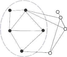
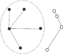(a) Partition $P=(S,S^{\prime})$ (b) Spn. forest in $P=(S,S^{\prime})$

Figure 2: Partitions and spanning forests of a graph.

Having thus far established that nodes with higher $\mathcal{C}^{*}(i)$, are more structurally central in the network, we now turn to average connectedness of nodes in this section. To show how structural centralities of nodes capture their immunity/vulnerability to random failures in the network, we study their connectedness in all the bi-partitions of a graph.

5.1 Connected Bi-partitions

Definition 5

Bi-partition $(P=(S,S^{\prime}))$: A cut of the graph $G$ which contains exactly two mutually exclusive and exhaustive connected subgraphs $S$ and $S^{\prime}$.

Let, $V(S)$ and $V(S^{\prime})$ be the mutually exclusive and exhaustive subsets of $V(G)$, $E(S)$ and $E(S^{\prime})$, the sets of edges in the respective components $S$ and $S^{\prime}$ of $P$ and $E(S,S^{\prime})$, the set of edges that violate $P$ i.e. have one end in $S$ and the other in $S^{\prime}$. Also, let $\mathcal{T}(S)$ and $\mathcal{T}(S^{\prime})$ be the set of spanning trees in the respective component sets $S$ and $S^{\prime}$. We denote by $\mathcal{P}(G)$, the set of all bi-partitions of $G(V,E)$. Clearly, a given $P=(S,S^{\prime})$ represents a state of the network in which $E(S,S^{\prime})$ have failed. A node $i\in V(S)$ stays connected to $|V(S)|-1$ nodes and gets disconnected from $|V(S^{\prime})|$ nodes. In the following relationship we show how topological centrality of node $i$ is related to a weighted sum of $|V(S)^{\prime}|$ over all the bi-partitions $P\in\mathcal{P}(G)$ of the network.

Theorem 3

$$l^{+}_{ii}\propto\sum_{P\in\mathcal{P}(G)}^{i\in V(S)}|\mathcal{T}(S)||\mathcal{T}(S^{\prime})||V(S^{\prime})|$$ (13)

Proof sketch: The following result, due to Chebotarev et al. [9, 10], forms the basis of our proof. Let $\mathcal{F}_{x}$ be the set of spanning rooted forests of $G(V,E)$ with $x$ edges. Precisely, $F_{x}\in\mathcal{F}_{x}$, is a spanning acyclic subgraph of $G$ with the same node set as $G$ and is composed of exactly $n-x$ trees with one node marked as a root in each of these $x$ trees. Let $\mathcal{F}^{ii}_{x}$, be the subset of $\mathcal{F}_{x}$ in which node $i$ is the root of the tree in which it belongs. Then,

$$l^{+}_{ii}=\frac{\varepsilon(\mathcal{F}^{ii}_{n-2})-\frac{1}{n}\varepsilon(\mathcal{F}_{n-2})}{\varepsilon(\mathcal{F}_{n-1})}$$ (14)

Here, $\varepsilon(\cdot)$ simply represents the cardinality of the input set (see [9, 10] for details). It is easy to see that $\varepsilon(\mathcal{F}_{n-1})=n|T(G)|$, as a spanning forest with $n-1$ edges is a spanning tree, and each spanning tree has exactly $n$ possible choices of roots. Also, $\varepsilon(\mathcal{F}_{n-2})$ and $\varepsilon(\mathcal{F}_{n-1})$ are invariants over the set of vertices $V(G)$ for a given graph. Hence, $l^{+}_{ii}\propto\varepsilon(\mathcal{F}^{ii}_{n-2})$. The rest of the proof follows from the results of the following lemmas:

Lemma 1

Let $\mathcal{F}^{ii}_{n-2|P}$ be the set of spanning forests with $n-2$ edges (or exactly two trees) rooted at node $i$ in a given bi-partition $P=(S,S^{\prime})$ and $\mathcal{T}(S)$, $\mathcal{T}(S^{\prime})$ be the set of spanning trees in $S$ and $S^{\prime}$ respectively. If $i\in V(S)$ then,

$$\varepsilon(\mathcal{F}^{ii}_{n-2|P})=|\mathcal{T}(S)|~{}|\mathcal{T}(S^{\prime})|~{}|V(S^{\prime})|$$

Proof : Let $T_{1}\in\mathcal{T}(S)$ and $T_{2}\in\mathcal{T}(S^{\prime})$. Clearly, $|E(T_{1})|=|V(S)|-1$ and $|E(T_{2})|=|V(S^{\prime})|-1$. As $|V(S)|+|V(S^{\prime})|=|V(G)|$ and $|E(T_{1})\cap E(T_{2})|=0$, $|E(T_{1})\cup E(T_{2})|=|V(S)|-1+|V(S^{\prime})|-1=n-2$. Each such pair $(T_{1},T_{2})$ is a spanning forest of $n-2$ edges. Given $i$ is the root of $T_{1}$ in $S$, we can choose $|V(S^{\prime})|$ roots for $T_{2}$ in $S^{\prime}$. There being $|\mathcal{T}(S)|~{}|\mathcal{T}(S^{\prime})|$ such pairs: $\varepsilon(\mathcal{F}^{ii}_{n-2|P})=|\mathcal{T}(S)|~{}|\mathcal{T}(S^{\prime})|~{}|V(S^{\prime})|$.

$\square$

By symmetry, for $j\in V(S^{\prime}):$

$$\varepsilon(\mathcal{F}^{jj}_{n-2|P})=|\mathcal{T}(S)|~{}|\mathcal{T}(S^{\prime})|~{}|V(S)|$$

Lemma 2

Given $\mathcal{P}(G)$, the set of all bi-partitions of $G$:

$$\varepsilon(\mathcal{F}^{ii}_{n-2})=\sum_{P\in\mathcal{P}(G)}^{i\in V(S)}|\mathcal{T}(S)||\mathcal{T}(S^{\prime})||V(S^{\prime})|$$

Proof: By definition, $\forall F\in\mathcal{F}_{n-2}$, $F$ belongs to exactly one of the partitions of $G$. Hence, $\mathcal{F}^{ii}_{n-2}=\coprod_{P\in\mathcal{P}}\varepsilon(\mathcal{F}^{ii}_{n-2|P})$. As the RHS is a disjoint union, counting members on both sides we obtain the proof.

$\square$

Evidently, combining the results of the two lemmas above, we obtain the proof for Theorem 3.

$\square$

To paraphrase, given a bi-partition $P=(S,S^{\prime})\in\mathcal{P}(G)$, such that $i\in V(S)$ and $j\in V(S^{\prime})$, Lemma 1 yields: $\varepsilon(\mathcal{F}^{ii}_{n-2|P})/\varepsilon(\mathcal{F}^{jj}_{n-2|P})=|V(S^{\prime})|/|V(S)|$. Clearly, for a given bi-partition, nodes in the larger of the two components of $P$ have a lower number of spanning forests rooted at them than those in the smaller component and vice versa. By extension,

$$l^{+}_{ii}-l^{+}_{jj} \propto \sum_{P\in\mathcal{P}(G)}^{i\in V(S),j\in V(S^{\prime})}|\mathcal{T}(S)||\mathcal{T}(S^{\prime})|(|V(S^{\prime})|-|V(S)|)$$

can be interpreted as a comparative measure of connectedness of nodes $i$ and $j$. Note that for $P\in\mathcal{P}(G)$, the RHS of (5.1) is zero when nodes $i$ and $j$ belong to the same component of $P$ or if $|V(S)|=|V(S^{\prime})|$ and positive when $i\in V(S),j\in V(S^{\prime})$ and $|V(S^{\prime})|>|V(S)|$ or vice versa. Therefore, a node $i$ with higher topological centrality stays connected to a greater number of nodes on an average in a disconnected network, than one with lower topological centrality and is consequently more immune to random edge failures in the network.

By simple extension, Kirchhoff index represents the average connectedness of all the nodes when a failure of a subset of edges partitions the network into two halves, thereby truly reflecting overall network robustness. It is easy to demonstrate that of all trees of order $n$, the star has the lowest Kirchhoff index and the root of the star has highest $\mathcal{C}^{*}(i)$ value. Also, amongst all graphs of order $n$ with differing volumes, the completely connected graph $K_{n}$ has the lowest Kirchhoff index.

5.2 A Case Study: When the Graph is a Tree

We now study the special case of trees. Recall, a tree $T(V,E)$ of order $n=|V(T)|$ is a connected acyclic graph with exactly $n-1=|E(T)|$ edges. As each of the $n-1$ edges $e_{ij}\in E(T)$, upon deletion produces a unique partition $P(S,S^{\prime})\in\mathcal{P}(T)$, we conclude that there are exactly $n-1$ connected bi-partitions of a tree. Moreover, the two sub-graphs $S$ and $S^{\prime}$ are also trees themselves, such that $|\mathcal{T}(S)|=|\mathcal{T}(S^{\prime})|=1$ for any partition $P(S,S^{\prime})$. For the nodes of the tree, we then obtain an elegant closed form for topological centrality in the following corollary.

Corollary 1

$$l^{+}_{ii}=\frac{1}{n^{2}}\sum_{P\in\mathcal{P}(T)}^{i\in V(S)}|V(S^{\prime})|^{2}$$ (15)

Proof: The proof follows simply by making the following observations about trees: $\varepsilon(\mathcal{F}_{n-1})=n\cdot 1=n$. Also,

$$\varepsilon(\mathcal{F}^{ii}_{n-2})=\sum_{P(S,S^{\prime})\in\mathcal{P}(G)}^{i\in V(S)}|V(S^{\prime})|$$ (16)

and

$$\varepsilon(\mathcal{F}_{n-2})=\sum_{P(S,S^{\prime})\in\mathcal{P}(G)}|V(S)||V(S^{\prime})|=\sum_{P(S,S^{\prime})\in\mathcal{P}(G)}(n-|V(S^{\prime})|)|V(S^{\prime})|$$ (17)

Thus substituting these values in $(\ref{equ:DenseSRFs})$, we obtain the proof.

$\square$

More importantly, in a tree, the shortest path distance $SPD(i,j)$ and the effective resistance distance $\Omega_{ij}$ between the node pair $(i,j)$ is exactly the same i.e.

$$SPD(i,j)=\Omega_{ij}=l^{+}_{ii}+l^{+}_{jj}-l^{+}_{ij}-l^{+}_{ji}$$ (18)

The result above is simply due to the fact that a tree is an acyclic graph. It is easy to see that

$$l^{+}_{ii}=\sum_{j=1}^{n}SPD(i,j)-Tr(\mathbf{L}^{+})~{}~{}~{}~{}\Rightarrow~{}~{}~{}~{}l^{+}_{ii}\propto\sum_{j=1}^{n}SPD(i,j)$$ (19)

But the node $i^{*}\in V(T)$ for which $\sum_{j=1}^{n}SPD(i^{*},j)$ is the least, is the so called tree center of $T$. Thus the node with the highest topological centrality, is also the tree center if the graph is a tree; a result which further knits our centrality measure into the broader body of knowledge (c.f. [25]).

6 Empirical Evaluations

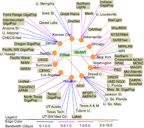
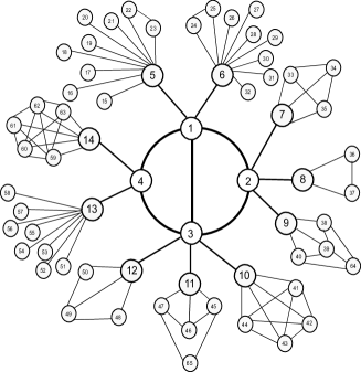
(a) Abilene Topology (b) Simulated topology (c) Perturbations

Figure 3: Abilene Network and a simulated topology.

Figure 4: Max-normalized centralities for simulated topology.

In this section, we empirically study the properties of topological centrality $(\mathcal{C}^{*}(i))$ and Kirchhoff index (we use $\mathcal{K}^{*}=\mathcal{K}^{-1}$ henceforth to maintain higher is better). We first show in §6.1, how a rank-order of nodes in terms of their topological centralities captures their structural roles in the network and then in §6.2 demonstrate how it, along with Kirchhoff index, is appropriately sensitivity to rewirings and local perturbations in the network.

6.1 Identifying Structural Roles of Nodes

Consider the router level topology of the Abilene network (Fig. 3(a)) [1]. At the core of this topology, is a ring of $11$ POP’s, spread across mainland US, through which several networks interconnect. Clearly, the connectedness of such a network is dependent heavily on the low degree nodes on the ring. For illustration, we mimic the Abilene topology, with a simulated network (Fig. 3(b)) which has a 4-node core $\{v_{1},...,v_{4}\}$ that connects $10$ networks through gateway nodes $\{v_{5},...,v_{14}\}$ (Fig.3(b)).

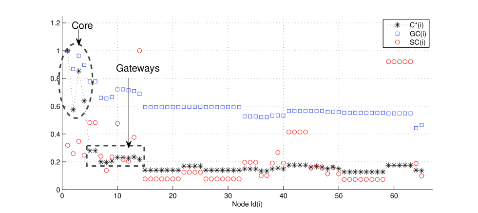
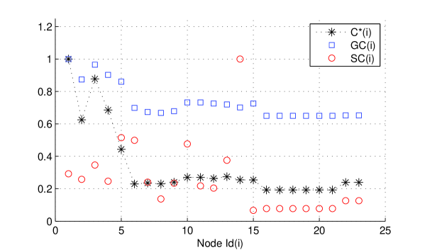
Fig. 4 shows the (max-normalized) values of geodesic closeness $(GC)$, subgraph centrality $(SC)$ and topological centrality $\mathcal{C}^{*}$ for the core $\{v_{1},...,v_{4}\}$, gateway $\{v_{5},...,v_{14}\}$ and other nodes $\{v_{15},...,v_{65}\}$ in topology (Fig.3(b)). Notice that $v_{5}$ and $v_{6}$, two of the gateway nodes in the topology, have the highest values of degree in the network i.e. $(d(v_{5})=d(v_{6})=10)$ while $v_{14}$ has the highest subgraph centrality $(SC)$. In contrast, $\mathcal{C}^{*}(i)$ ranks the four core nodes higher than all the gateway nodes with $v_{1}$ at the top. The relative peripherality of $v_{5},v_{6}$ and $v_{14}$ as compared to the core nodes requires no elaboration. As far as geodesic centrality $(GC)$ is concerned, it ranks all the nodes in the subnetwork abstracted by $v_{5}$, namely $v_{15}-v_{23}$, as equals even though $v_{22}$ and $v_{23}$ have redundant connectivity to the network through each other and are, ever so slightly, better connected than the others - a property reflected in their $\mathcal{C}^{*}(i)$ rankings.

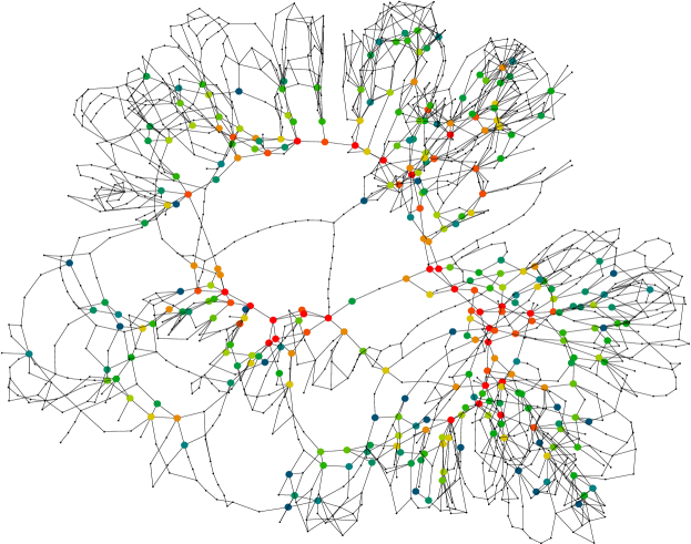
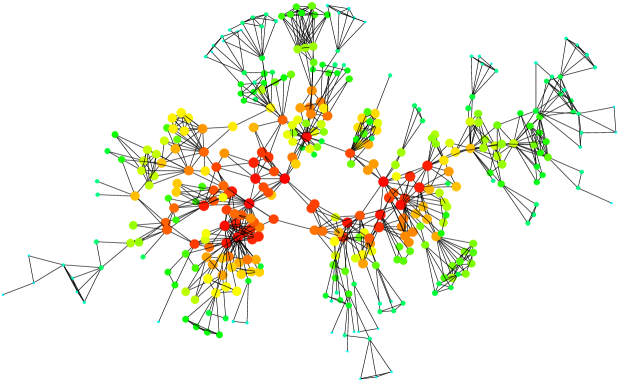
We see similar characterization of structural roles of nodes in two real world networks in terms of structural centrality: the western states power-grid network [40] and a social network of co-authorships [31], as shown through a color scheme based on $\mathcal{C}^{*}(i)$ values in Fig. 5. Core-nodes connecting different sub-communities of nodes in both these real world networks are recognized effectively by topological centrality as being more central ($Red$ end of the spectrum) than several higher degree peripheral nodes.

(a) The western-states power grid network [40] (b) A network of co-authorships in network sciences [31]

Figure 5: Real world networks: $Red\rightarrow Turqoise$ in order of decreasing $\mathcal{C}^{*}(i)$.

6.2 Sensitivity to Local Perturbations

(a) Vis-à-vis centralities (b) Vis-à-vis betweennesses

Figure 6: PERT-I: Max-normalized values of centralities and betweennesses for core, gateway and some other nodes.

An important property of centrality measures is their sensitivity to perturbations in network structure. Traditionally, structural properties in real world networks have been equated to average statistical properties like power-law/scale-free degree distributions and rich club connectivity [2, 15, 16]. However, the same degree sequence $D=\{d(1)\geq d(2)\geq...\geq d(n)\}$, can result in graphs of significantly varying topologies. Let $\mathcal{G}(D)$ be the set of all connected graphs with scaling sequence $D$. The generalized Randić index $R_{1}(G)$ [6, 37]:

$$R_{1}(G)=\sum_{e_{ij}\in E(G)}d(i)d(j)$$ (20)

where $G\in\mathcal{G}(D)$, is considered to be a measure of overall connectedness of $G$. Higher $R_{1}(G)$ suggests that nodes of higher degrees connect with each other with high probability thereby displaying the so-called rich club connectivity (RCC) in $G$ [27]. Similarly, the average of each centrality/betweenness index ($GC,SC,GB,RB$ averaged over the set of nodes), is in itself a global structural descriptor for the graph $G$ [14]. We now examine the sensitivity of each index with respect to local perturbations in the subnetwork abstracted by the core node $v_{1}$ and its two gateway neighbors $v_{5}$ and $v_{6}$.

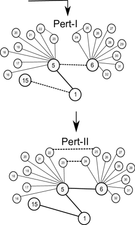
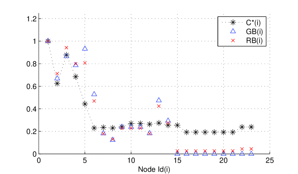
First, we rewire edges $e_{15,5}$ and $e_{6,1}$ to $e_{15,1}$ and $e_{6,5}$ respectively (PERT-I Fig. 3(c)). PERT-I is a degree preserving rewiring which only alters local connectivities i.e. neither individual node degrees nor average node degree changes. Fig. 6(a) and (b) respectively show the altered values of centralities $(\mathcal{C}^{*},GC,SC)$ and betweennesses, geodesic and random-walk i.e. $(GB,RB)$, after PERT-I. Note, after PERT-I, $v_{15}$ is directly connected to $v_{1}$ which makes $\mathcal{C}^{*}(v_{15})$ comparable to other gateway nodes while $SC(v_{15}),GB(v_{15}),RB(v_{15})$ seem to be entirely unaffected. Moreover, PERT-I also results in $v_{6}$ losing its direct link to the core, reflected in the decrease in $\mathcal{C}^{*}(v_{6})$ and a corresponding increase in $\mathcal{C}^{*}(v_{5})$. $\mathcal{C}^{*}(i)$, however, still ranks the core nodes higher than $v_{5}$ (whereas $SC,GB,RB$ do not) because PERT-I being a local perturbation should not affect nodes outside the sub-network — $v_{1}$ continues to abstract the same sub-networks from the rest of the topology. We, therefore, observe that $\mathcal{C}^{*}(i)$ is appropriately sensitive to the changes in connectedness of nodes in the event of local perturbations. But what about the network on a whole?

Table 1: Sensitivity to local perturbations, $\overline{X}=1/n\sum_{i}^{n}X(i)$: Avg. node centrality for a network.

$\#$	Structural Descriptor	PERT-I	PERT-II
1	$\mathcal{K}^{*}(G)$ (or $\overline{\mathcal{C}^{*}}$)	$\downarrow$	$\uparrow$
2	$R_{1}(G)$	$\uparrow$	$\leftrightarrow$
3	$\overline{GC}$	$\downarrow$	$\uparrow$
4	$\overline{SC}$, $\overline{GB}$	$\uparrow$	$\downarrow$
5	$\overline{RB}$	$\uparrow$	$\uparrow$

Let $G$ and $G_{1}$ be the topologies before and after PERT-I. $G_{1}$ is less well connected overall than $G$ as the failure of $e_{5,1}$ in $G_{1}$ disconnects $19$ nodes from the rest of the network as compared to $10$ nodes in $G$. However,

$$\Delta R_{1}(G\rightarrow G_{1})=\frac{R_{1}(G_{1})-R_{1}(G)}{R_{1}(G)}=0.029$$

as the two highest degree nodes ($v_{5}$ and $v_{6}$) are directly connected in $G_{1}$ (see TABLE 1 for the sensitivity of other centrality based global structural descriptors). In contrast, $\Delta\mathcal{K}^{*}(G\rightarrow G_{1})=-0.045$, which rightly reflects the depreciation in overall connectedness after PERT-I (recall $\mathcal{K}^{*}(G)=\mathcal{K}^{-1}(G$). Table 1 shows the changes in the average of all centrality and betweenness indices post PERT-I.

A subsequent degree preserving perturbation PERT-II of $G_{1}$, rewiring $e_{22,23}$ and $e_{24,25}$ to $e_{22,25}$ and $e_{23,24}$, to obtain $G_{2}$, creates two cycles in $G_{2}$ that safeguard against the failure of edge $e_{5,6}$. This significantly improves local connectivities in the sub-network. However, $\Delta R_{1}(G_{1}\rightarrow G_{2})=0$ (and average $SC$ decreases) while $\Delta\mathcal{K}^{*}(G_{1}\rightarrow G_{2})=0.036$ which once again shows the efficacy of Kirchhoff index as a measure of global connectedness of networks.

7 A Word on Computational Complexity

We now discuss the practical aspects of computing the topological centrality measure for the set of nodes in the graph representing the complex network. It suffices to compute the pseudo-inverse of the matrix $\mathbf{L}$, the Laplacian, to obtain the matrix $\mathbf{L}^{+}$. The most common method for computing the pseudo-inverse of a matrix mathematically, is to use the singular value decomposition (SVD). Indeed, mathematical software such as Matlab, come equipped with subroutines, such as pinv (for pseudo-inverse), which make use of the SVD factorization. It is common knowledge that the computational complexity for the SVD method is, in terms of worst case complexities, $O(n^{3})$ where $n$ is the number of rows/columns of the matrix. Thus the base worst case complexity for computing the topological centrality measure is indeed $O(n^{3})$, where $n$ is the order of the graph. This worst case complexity is at par with the competitive centrality measures, like geodesic centrality $(GC)$ and betweenness $(GB)$ (based on shortest paths) as well as subgraph centrality $(SC)$; and better than the random-walk betweenness $(RB)$ (see Table 2).

However, given that graphs (or networks abstracted as graphs), are topological objects, and the nature of the eigen spaces of the matrices $\mathbf{L}$ and $\mathbf{L}^{+}$ (as discussed in §3), we can be clever from the computational point of view. Although a full discussion of these computational improvisations is out of the scope of the current work, we provide some useful pointers for the interested reader. Exploiting the fact that $\lambda_{n}=0$, the smallest eigen value of $\mathbf{L}$, is unique if the network is connected, it has been shown in [41] that $\mathbf{L}^{+}$ can be computed by perturbing the matrix $\mathbf{L}$ (by adding a constant $1/n$ to every element) which yields an invertible full rank matrix. This method, though considerably faster in practice on Matlab, still leaves the worst case complexity at $O(n^{3})$.

In [19], we find a way of approximating $\mathbf{L}^{+}$ by using fast converging Monte-Carlo algorithms. Such parallel algorithms exploit the sparsity of real world networks which in turn makes the Laplacian $\mathbf{L}$ a sparse matrix (even though $\mathbf{L}^{+}$ is always full). However, we observe that from the point of view of computing topological centrality alone $(\mathcal{C}^{*}(i))$, all we need is the diagonal of $\mathbf{L}^{+}$. It is known that subsets of inverse for a sparse matrix can be computed to a given pattern (selective elements), using parallel and multi-frontal approaches (c.f. [8] and the references therein).

Finally, another interesting result has recently been proposed in [28] that shows that as the density of edges in the network increases, the hitting time from node $i$ to $j$ can be well approximated as $H_{ij}\approx Vol(G)d(i)^{-1}$. By extension, the commute time becomes $C_{ij}\approx Vol(G)(d(i)^{-1}+d(j)^{-1})$. So for dense graphs, we can compute topological centrality for nodes using the node degree distribution alone (see §4). Most importantly, this result implies that topological centrality, which is a measure of the overall position and connectedness of a node, is determined entirely by its local connectedness determined by its degree, a remarkable result indeed.

8 Conclusion and Future Work

In this work, we presented a geometric perspective on robustness in complex networks in terms of the Moore-Penrose pseudo-inverse of the graph Laplacian. We proposed topological centrality $(\mathcal{C}^{*}(i))$ and Kirchhoff index $(\mathcal{K}(G))$ that respectively reflect the length of the position vector for a node and the overall volume of the graph embedding and therefore are suitable geometric measures of robustness of individual nodes and the overall network. Additionally, we provided interpretations for these indices in terms of the overhead incurred in random detours through a node in question as well as in terms of the recurrence probabilities and voltage distribution in the EEN corresponding to the network. Both indices reflect the global connectedness properties of individual nodes and the network on a whole, particularly in the event of multiple edge failures that may render the network disconnected. Through numerical analysis on simulated and real world networks, we demonstrated that $\mathcal{C}^{*}(i)$ captures structural roles played by nodes in networks and, along with Kirchhoff index, is suitably sensitive to perturbations/rewirings in the network. In terms of computational complexity, topological centrality compares well with other geodesic and all-paths based indices in literature (see Table 2) and performs better than random-walk betweenness in the asymptotic case. In future, we aim at investigating similar metrics for the case of strongly connected weighted directed graphs to further generalize our work, a preliminary attempt towards which has already begun in the form of the results in [5].

Table 2: Taxonomy and computational complexities of centrality measures (for all nodes).

# Measure Paths covered Complexity 1. Degree - $O(m)$ 2. $GC$, $GB$ Geodesic paths $O(n^{3})$ 3. $\mathcal{C}^{*}$ All paths $O(n^{3})$ 4. $SC$ All paths $O(n^{3})$ 5. $RB$ All paths $O(m+n)n^{2}$ 6. $FB$ All paths $O(m^{2}n)$

9 Acknowledgment

We express our sincere gratitude towards the anonymous reviewers whose suggestions helped improve the quality of this work. This research was supported in part by DTRA grant HDTRA1-09-1-0050 and NSF grants CNS-0905037, CNS-1017647 and CNS-1017092.

References

- [1] www.stanford.edu/services/internet2/abilene.html.
- [2] R. Albert, H. Jeong, and A. L. Barabási. Error and attack tolerance of complex networks. Nature, 406(6794):378–382, 2000.
- [3] A. Ben-Israel and T. Greville. Generalized Inverses: Theory and Applications, edition. Springer-Verlag, 2003.
- [4] E. Bendito, A. Carmona, A. M. Encinas, J. M. Gesto, and M. Mitjana. Kirchhoff indexes of a network. Linear Algebra and its Applications, 432(9):2278–2292, 2010.
- [5] D. Boley, G. Ranjan, and Z.-L. Zhang. Commute times for a directed graph using an asymmetric laplacian. Linear Algebra and its Applications, 435.
- [6] B. Bollobás and P. Erdős. Graphs of extremal weights. Ars Combin., 50:225–233, 1998.
- [7] S. P. Borgatti. Centrality and network flow. Social Networks, 27(1):55–71, 2005.
- [8] Y. E. Campbell and T. A. Davis. Computing the sparse inverse subset: An inverse multifrontal approach. Tech. report TR-95-021, Comp. and Inf. Sciences Dept., Univ. of Florida, Gainesville, 1995.
- [9] P. Chebotarev and E. Shamis. The matrix-forest theorem and measuring relations in small social groups. Automation and Remote Control, 58(9):1505–1514, 1997.
- [10] P. Chebotarev and E. Shamis. On proximity measures for graph vertices. Automation and Remote Control, 59(10):1443–1459, 1998.
- [11] S. N. Dorogovtsev, A. V. Goltsev, J. F. F. Mendes, and A. N. Samukhin. Spectra of complex networks. Physical Review E, 68(4), 2003.
- [12] P. G. Doyle and J. L. Snell. Random Walks and Electric Networks. The Math. Assoc. of America, 1984.
- [13] E. Estrada and N. Hatano. A vibrational approach to node centrality and vulnerability. Physica A, 389, 2010.
- [14] E. Estrada and J. A. Rodríguez-Velázquez. Subgraph centrality in complex networks. Phys. Review E, 71, 2005.
- [15] M. Faloutsos, P. Faloutsos, and C. Faloutsos. On power-law relationships of the internet topology. In Proc. of the ACM SIGCOMM, pages 251–262, 1999.
- [16] I. J. Farkas, I. Derényi, A. L. Barabási, and T. Vicsek. Spectra of real world graphs: Beyond the semicircle law. Physical Review E, 64(2), 2001.
- [17] M. Fiedler. Algebraic connectivity of graphs. Czechoslovak Math. J., 23:298–305, 1973.
- [18] M. Fiedler. A property of eigenvectors of nonnegative symmetric matrices and its applications to graph theory. Czechoslovak Math. J., 25(100):619–633, 1975.
- [19] F. Fouss, A. Pirotte, J. M. Renders, and M. Saerens. Random-walk computation of similarities between nodes of a graph with application to collaborative recommendation. IEEE Transactions on Knowledge and Data Engineering, 19, 2007.
- [20] L. C. Freeman. A set of measures of centrality based upon betweenness. Sociometry, 40:35–41, 1977.
- [21] L. C. Freeman. Centrality in social networks: Conceptual clarification. Social Networks, 1:215–239, 1979.
- [22] L. C. Freeman, S. P. Borgatti, and D. R. White. Centrality in valued graphs: A measure of betweenness based on network flow. Social Networks, 13:141–154, 1991.
- [23] F. Gobel and A. Jagers. Random walks on graphs. Stochastic Processes and Their Applications, 2:311–336, 1974.
- [24] J. G. Kemeny, J. L. Snell, and A. W. Knapp. Denumerable Markov Chains. Van Nostrand, New York, 1966.
- [25] S. J. Kirkland, M. Neumann, and B. L. Shader. Distances in weighted trees and group inverse of laplacian matrices. SIAM Journal of Matrix Anal. Appl., 18.
- [26] D. J. Klein and M. Randić. Resistance distance. J. Math. Chemistry, 12:81–95, 1993.
- [27] L. Li, D. Alderson, W. Willinger, and J. Doyle. A first-principles approach to understanding the internet’s router-level topology. In Proc. of the ACM SIGCOMM, 2004.
- [28] U. V. Luxburg, A. Radl, and M. Hein. Getting lost in space: Large sample analysis of the commute distance. NIPS, 2010.
- [29] M. Mitrović and B. Tadić. Spectral and dynamical properties in classes of sparse networks with mesoscopic inhomogeneities. Physical Review E, 80, 2009.
- [30] M. E. J. Newman. A measure of betweenness centrality based on random walks. Social Networks, 27(1):39–54, 2005.
- [31] M. E. J. Newman. Finding community structure in networks using the eigenvectors of matrices. Preprint Physics/0605087, 2006.
- [32] J. D. Noh and H. Rieger. Random walks on complex networks. Phys. Rev. Lett., 92, 2004.
- [33] J. L. Palacios. Closed-form formulas for kirchhoff index. Intl. Journal of Quantum Chemistry, 81:135–140, 2001.
- [34] J. L. Palacios. Resistance distance in graphs and random walks. Intl. Journal of Quantum Chemistry, 81:29–33, 2001.
- [35] J. L. Palacios. On the kirchhoff index of regular graphs. Intl. Journal of Quantum Chemistry, 110:1307–1309, 2010.
- [36] J. L. Palacios and J. M. Renom. Bounds for the kirchhoff index of regular graphs via the spectra of their random walks. Intl. Journal of Quantum Chemistry, 110:1637–1641, 2010.
- [37] M. Randić. On characterization of molecular branching. J. Amer. Chem. Society, 97:6609–6615, 1975.
- [38] K. A. Stephenson and M. Zelen. Rethinking centrality: Methods and examples. Social Networks, 11:1–37, 1989.
- [39] P. Tetali. Random walks and effective resistance of networks. Journal of Theoretical Probability, pages 101–109, 1991.
- [40] D. J. Watts and S. H. Strogatz. Collective dynamics of ‘small-world’ networks. Nature, 393:440–442, 1998.
- [41] W. Xiao and I. Gutman. Resistance distance and laplacian spectrum. Theoretical Chemistry Accounts, 110:284–289, 2003.
- [42] B. Zhou and N. Trinajstić. A note on kirchhoff index. Chemical Physics Letters, 455(1-3):120–123.