GraphLab: A Distributed Framework for
Machine Learning in the
Cloud
Abstract
Machine Learning (ML) techniques are indispensable in a wide range of fields. Unfortunately, the exponential increase of dataset sizes are rapidly extending the runtime of sequential algorithms and threatening to slow future progress in ML. With the promise of affordable large-scale parallel computing, Cloud systems offer a viable platform to resolve the computational challenges in ML. However, designing and implementing efficient, provably correct distributed ML algorithms is often prohibitively challenging. To enable ML researchers to easily and efficiently use parallel systems, we introduced the GraphLab abstraction which is designed to represent the computational patterns in ML algorithms while permitting efficient parallel and distributed implementations.
In this paper we provide a formal description of the GraphLab parallel abstraction and present an efficient distributed implementation. We conduct a comprehensive evaluation of GraphLab on three state-of-the-art ML algorithms using real large-scale data and a 64 node EC2 cluster of 512 processors. We find that GraphLab achieves orders of magnitude performance gains over Hadoop while performing comparably or superior to hand-tuned MPI implementations.
1 Introduction
With the exponential growth in Machine Learning (ML) datasets sizes and increasing sophistication of ML techniques, there is a growing need for systems that can execute ML algorithms efficiently in parallel on large clusters. Unfortunately, based on our comprehensive survey, we find that existing popular high level parallel abstractions, such as MapReduce [1, 2] and Dryad [3], do not efficiently fit many ML applications. Alternatively, designing, implementing, and debugging ML algorithms on low level frameworks such as OpenMP [4] or MPI [5] can be excessively challenging, requiring the user to address complex issues like race conditions, deadlocks, and message passing in addition to the already challenging mathematical code and complex data models common in ML research.
In this paper we describe the culmination of two years of research in collaboration with ML, Parallel Computing, and Distributed Systems experts. By focusing on Machine Learning we designed GraphLab, a domain specific parallel abstraction [6] that fits the needs of the ML community, without sacrificing computational efficiency or requiring ML researchers to redesign their algorithms. In [7] we first introduced the GraphLab multi-core API to the ML community.
In this paper we build upon our earlier work by refining the GraphLab abstraction and extending the GraphLab API to the distributed setting. We provide the first formal presentation of the streamlined GraphLab abstraction and describe how the abstraction enabled us to construct a highly optimized C++ API for the distributed setting. We conduct a comprehensive performance analysis on the Amazon Elastic Cloud (EC2) cloud computing service. We show that applications created using GraphLab outperform equivalent Hadoop/MapReduce[1] implementations by 20-60x and match the performance of carefully constructed and fine tuned MPI implementations. Our main contributions are the following:
-
•
Asurvey of common properties of Machine Learning algorithms and the limitations of existing parallel abstractions. (Sec. 2)
-
•
A formal presentation of the GraphLab abstraction and how it naturally represents ML algorithms. (Sec. 3)
-
•
Two efficient distributed implementations of the GraphLab abstraction (Sec. 4):
-
Chromatic Engine: uses graph coloring to achieve efficient sequentially consistent execution for static schedules.
-
Locking Engine: uses distributed locking and latency hiding to achieve sequential consistency while supporting prioritized execution.
-
-
•
Implementations of three state-of-the-art machine learning algorithms using the GraphLab abstraction. (Sec. 5)
-
•
An extensive evaluation of GraphLab using a 512 processor (64 node) EC2 cluster, including comparisons to Hadoop and MPI implementations. (Sec. 6)
2 A Need for GraphLab in ML
| Computation Model | Sparse Depend. | Async. Comp. | Iterative | Prioritized Ordering | Sequentially Consistent | Distributed | |
| MPI[5] | Messaging | Yes | Yes | Yes | N/A | N/A | Yes |
| MapReduce[1] | Par. data-flow | No | No | extensions | N/A | N/A | Yes |
| Dryad[3] | Par. data-flow | Yes | No | extensions | N/A | N/A | Yes |
| Pregel[8]/BPGL[9] | GraphBSP[10] | Yes | No | Yes | N/A | N/A | Yes |
| Piccolo[11] | Distr. map | N/A | Yes | Yes | No | accumulators | Yes |
| Pearce et.al.[12] | Graph Visitor | Yes | Yes | Yes | Yes | No | No |
| GraphLab | GraphLab | Yes | Yes | Yes | Yes | Yes | Yes |
The GraphLab abstraction is the product of several years of research in designing and implementing systems for statistical inference in probabilistic graphical models. Early in our work [16], we discovered that the high-level parallel abstractions popular in the ML community such as MapReduce [1, 2] and parallel BLAS [17] libraries are unable to express statistical inference algorithms efficiently. Our work revealed that an efficient algorithm for graphical model inference should explicitly address the sparse dependencies between random variables and adapt to the input data and model parameters.
Guided by this intuition we spent over a year designing and implementing various machine learning algorithms on top of low-level threading primitives and distributed communication frameworks such as OpenMP [4], CILK++ [18] and MPI [5]. Through this process, we discovered the following set of core algorithmic patterns that are common to a wide range of machine learning techniques. Following, we detail our findings and motivate why a new framework is needed (see Table 1).
Sparse Computational Dependencies: Many ML algorithms can be factorized into local dependent computations which examine and modify only a small sub-region of the entire program state. For example, the conditional distribution of each random variable in a large statistical model typically only depends on a small subset of the remaining variables in the model. This computational sparsity in machine learning arises naturally from the statistical need to reduce model complexity.
Parallel abstractions like MapReduce [1] require algorithms to be transformed into an embarrassingly parallel form where computation is independent. Unfortunately, transforming ML algorithms with computational dependencies into the embarrassingly parallel form needed for these abstractions is often complicated and can introduce substantial algorithmic inefficiency [19]. Alternatively, data flow abstractions like Dryad [3], permit directed acyclic dependencies, but struggle to represent cyclic dependencies common to iterative ML algorithms. Finally, graph-based messaging abstractions like Pregel [8] provide a more natural representation of computational dependencies but require users to explicitly manage communication between computation units.
Asynchronous Iterative Computation: From simulating complex statistical models, to optimizing parameters, many important machine learning algorithms iterate over local computation kernels. Furthermore, many iterative machine learning algorithms benefit from [20, 21, 16] and in some cases require [22] asynchronous computation. Unlike synchronous computation, in which all kernels are computed simultaneously (in parallel) using the previous values for dependent parameters, asynchronous computation requires that the local computation kernels use the most recently available values.
Abstractions based on bulk data processing, such as MapReduce [1] and Dryad [3] were not designed for iterative computation. While recent projects like MapReduce Online [13], Spark [15], Twister [23], and Nexus [14] extend MapReduce to the iterative setting, they do not support asynchronous computation. Similarly, parallel graph based abstractions like Pregel [8] and BPGL [9] adopt the Bulk Synchronous Parallel (BSP) model [10] and do not naturally express asynchronous computation.
Sequential Consistency: By ensuring that all parallel executions have an equivalent sequential execution, sequential consistency eliminates many challenges associated with designing, implementing, and testing parallel ML algorithms. In addition, many algorithms converge faster if sequential consistency is ensured, and some even require it for correctness.
However, this view is not shared by all in the ML community. Recently, [24, 25] advocate soft-optimization techniques (e.g., allowing computation to intentionally race), but we argue that such techniques do not apply broadly in ML. Even for the algorithms evaluated in [24, 25], the conditions under which the soft-optimization techniques work are not well understood and may fail in unexpected ways on different datasets.
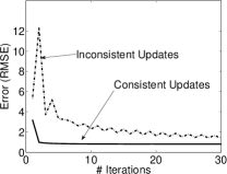
Indeed, for some machine learning algorithms sequential consistency is strictly required. For instance, Gibbs sampling [26], a popular inference algorithm, requires sequential consistency for statistical correctness, while many other optimization procedures require sequential consistency to converge (Fig. 1 demonstrates that the prediction error rate of one of our example problems is dramatically better when computation is properly asynchronous.). Finally, as [21] demonstrates, the lack of sequential consistency can dramatically increase the time to convergence for stochastic optimization procedures.
By designing an abstraction which enforces sequentially consistent computation, we eliminate much of the complexity introduced by parallelism, allowing the ML expert to focus on algorithm design and correctness of numerical computations. Debugging mathematical code in a parallel program which has random errors caused by non-deterministic ordering of concurrent computation is particularly unproductive.
The discussion of sequential consistency is relevant only to frameworks which support asynchronous computation. Piccolo [11] provides a limited amount of consistency by combining simultaneous writes using accumulation functions. However, this only protects against single write races, but does not ensure sequential consistency in general. The parallel asynchronous graph traversal abstraction by Pearce et. al. [12] does not support any form of consistency, and thus is not suitable for a large class of ML algorithms.
Prioritized Ordering: In many ML algorithms, iterative computation converges asymmetrically. For example, in parameter optimization, often a large number of parameters will quickly converge after only a few iterations, while the remaining parameters will converge slowly over many iterations [27, 28]. If we update all parameters equally often, we could waste substantial computation recomputing parameters that have effectively converged. Conversely, by focusing early computation on more challenging parameters first, we can potentially reduce computation.
Adaptive prioritization can be used to focus iterative computation where it is needed. The only existing framework to support this is the parallel graph framework by Pearce et. al. [12]. The framework is based on the visitor-pattern and prioritizes the ordering of visits to vertices. GraphLab however, allows the user to define arbitrary ordering of computation, and our implementation supports efficient FIFO and priority-based scheduling.
Rapid Development: Machine learning is a rapidly evolving field with new algorithms and data-sets appearing weekly. In many cases these algorithms are not yet well characterized and both the computational and statistical properties are under active investigation. Large-scale parallel machine learning systems must be able to adapt quickly to changes in the data and models in order to facilitate rapid prototyping, experimental analysis, and model tuning. To achieve these goals, an effective high-level parallel abstraction must hide the challenges of parallel algorithm design, including race conditions, deadlock, state-partitioning, and communication.
3 The GraphLab Abstraction
Using the ideas from the previous section, we extracted a single coherent computational pattern: asynchronous parallel computation on graphs with a sequential model of computation. This pattern is both sufficiently expressive to encode a wide range of ML algorithms, and sufficiently restrictive to enable efficient parallel implementations.
The GraphLab abstraction consists of three main parts, the data graph, the update function, and the sync operation. The data graph (Sec. 3.1) represents user modifiable program state, and both stores the mutable user-defined data and encodes the sparse computational dependencies. The update functions (Sec. 3.2) represent the factorized user computation and operate on the data graph by transforming data in small overlapping contexts called scopes. Finally, the sync operation (Sec. 3.3) is used to maintain global aggregate statistics of the data graph.
We now present the GraphLab abstraction in greater detail. To make these ideas more concrete, we will use the PageRank algorithm [29] as a running example. While PageRank is not a common machine learning algorithm, it is easy to understand and shares many properties common to machine learning algorithms.
Example 3.1 (PageRank).
The PageRank algorithm recursively defines the rank of a webpage :
| (3.1) |
in terms of the ranks of those pages that link to and the weight of the link as well as some probability of randomly jumping to that page. The PageRank algorithm, simply iterates Eq. (3.1) until the individual PageRank values converge (i.e., change by less than some small ).
3.1 Data Graph
The GraphLab abstraction stores the program state as an undirected graph called the data graph. The data graph is a container which manages the user defined data . Here we use the term “data” broadly to refer to model parameters, algorithmic state, and even statistical data. The user can associate arbitrary data with each vertex and edge in the graph. Since some machine learning applications require directed edge data (e.g., weights on directed links in a web-graph) we provide the ability to store and retrieve data associated with directed edges. While the graph data is mutable, the graph structure is static111Although we find that fixed structures are sufficient for most ML algorithms, we are currently exploring the use of dynamic graphs. and cannot be changed during execution.
Example (PageRank: Ex. 3.1).
The data graph for PageRank is directly obtained from the web graph, where each vertex corresponds to a web page and each edge represents a link. The vertex data stores , the current estimate of the PageRank, and the edge data stores , the directed weight of the link.
The data graph is convenient for representing the state of a wide range of machine learning algorithms. For example, many statistical models are efficiently represented by undirected graphs [30] called Markov Random Fields (MRF). The data graph is derived directly from the MRF, with each vertex representing a random variable. In this case the vertex data and edge data may store the local parameters that we are interested in learning.
3.2 Update Functions
Computation is encoded in the GraphLab abstraction via user defined update functions. An update function is a stateless procedure which modifies the data within the scope of a vertex and schedules the future execution of other update functions. The scope of vertex (denoted by ) is the data stored in , as well as the data stored in all adjacent vertices and edges as shown in Fig. 2.
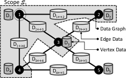
A GraphLab update function takes as an input a vertex and its scope and returns the new version of the scope as well as a set of tasks which encodes future task executions.
After executing an update function the modified scope data in is written back to the data graph. Each task in the set of tasks , is a tuple consisting of an update function and a vertex . All returned task are executed eventually by running following the execution semantics described in Sec. 3.4.
Rather than adopting a message passing or data flow model as in [8, 3], GraphLab allows the user defined update functions complete freedom to read and modify any of the data on adjacent vertices and edges. This simplifies user code and eliminates the need for the users to reason about the movement of data. By controlling what tasks are added to the task set, GraphLab update functions can efficiently express adaptive computation. For example, an update function may choose to reschedule its neighbors only when it has made a substantial change to its local data.
The update function mechanism allows for asynchronous computation on the sparse dependencies defined by the data graph. Since the data graph permits the expression of general cyclic dependencies, iterative computation can be represented easily.
Many algorithms in machine learning can be expressed as simple update functions. For example, probabilistic inference algorithms like Gibbs sampling [26], belief propagation [31], expectation propagation [32] and mean field variational inference [33] can all be expressed using update functions which read the current assignments to the parameter estimates on neighboring vertices and edges and then apply sampling or optimization techniques to update parameters on the local vertex.
Example (PageRank: Ex. 3.1).
The update function for PageRank (defined in Alg. 1) computes a weighted sum of the current ranks of neighboring vertices and assigns it as the rank of the current vertex. The algorithm is adaptive: neighbors are listed for update only if the value of current vertex changes more than a predefined threshold.
3.3 Sync Operation
In many ML algorithms it is necessary to maintain global statistics describing data stored in the data graph. For example, many statistical inference algorithms require tracking of global convergence estimators. Alternatively, parameter estimation algorithms often compute global averages or even gradients to tune model parameters. To address these situations, the GraphLab abstraction expresses global computation through the sync operation, which aggregates data across all vertices in the graph in a manner analogous to MapReduce. The results of the sync operation are stored globally and may be accessed by all update functions. Because GraphLab is designed to express iterative computation, the sync operation runs repeated at fixed user determined intervals to ensure that the global estimators remain fresh.
The sync operation is defined as a tuple consisting of a unique key, three user defined functions, an initial accumulator value, and an integer defining the interval between sync operations. The sync operation uses the Fold and Merge functions to perform a Global Synchronous Reduce where Fold aggregates vertex data and Merge combines intermediate Fold results. The Finalize function performs a transformation on the final value and stores the result. The Key can then be used by update functions to access the most recent result of the sync operation. The sync operation runs periodically, approximately every update function calls222The resolution of the synchronization interval is left up to the implementation since in some architectures a precise synchronization interval may be difficult to maintain..
Example (PageRank: Ex. 3.1).
We can compute the second most popular page on the web by defining the following sync operation:
Where the accumulator taking on the initial value as the empty array . The function “” returns the two pages with the highest pagerank in the set . After the global reduction, the acc array will contain the top two pages and in Finalize extracts the second entry. We may want to update the global estimate every vertex updates.
3.4 The GraphLab Execution Model
The GraphLab execution model, presented in Alg. 2, follows a simple single loop semantics. The input to the GraphLab abstraction consists of the data graph , an update function Update, an initial set of tasks to update, and any sync operations. While there are tasks remaining in , the algorithm removes (Line 2) and executes (Line 2) tasks, adding any new tasks back into (Line 2). The appropriate sync operations are executed whenever necessary. Upon completion, the resulting data graph and synced values are returned to the user.
The exact behavior of (Line 2) is up to the implementation of the GraphLab abstraction. The only guarantee the GraphLab abstraction provides is that RemoveNext removes and returns an update task in . The flexibility in the order in which RemoveNext removes tasks from provides the opportunity to balance features with performance constraints. For example, by restricting task execution to a fixed order, it is possible to optimize memory layout. Conversely, by supporting prioritized ordering it is possible to implement more advanced ML algorithms at the expense run-time overhead. In our implementation (see Sec. 4) we support fixed execution ordering (Chromatic Engine) as well as FIFO and prioritized ordering (Locking Engine).
The GraphLab abstraction presents a rich sequential model that is automatically translated into a parallel execution by allowing multiple processors to remove and execute update tasks simultaneously. To retain the same sequential execution semantics we must ensure that overlapping computation is not run simultaneously. However, the extent to which computation can safely overlap depends on the user defined update function. In the next section we introduce several consistency models that allow the runtime to optimize the parallel execution while maintaining consistent computation.
3.5 Sequential Consistency Models
A parallel implementation of GraphLab must guarantee sequential consistency [34] over update tasks and sync operations. We define sequential consistency in the context of the GraphLab abstraction as:
Definition 3.1 (GraphLab Sequential Consistency).
For every parallel execution of the GraphLab abstraction, there exists a sequential ordering on all executed update tasks and sync operations which produces the same data graph and synced global values.
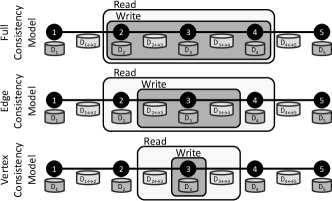
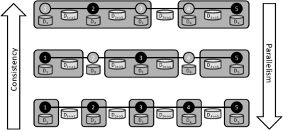
A simple method to achieve sequential consistency among update functions is to ensure that the scopes of concurrently executing update functions do not overlap. We refer to this as the full consistency model (see Fig. 3(a)). Full consistency limits the potential parallelism since concurrently executing update functions must be at least two vertices apart (see Fig. 3(b)). Even in moderately dense data graphs, the amount of available parallelism could be low. Depending on the actual computation performed within the update function, additional relaxations can be safely made to obtain more parallelism without sacrificing sequential consistency.
We observed that for many machine learning algorithms, the update functions do not need full read/write access to all of the data within the scope. For instance, the PageRank update in Eq. (3.1) only requires read access to edges and neighboring vertices. To provide greater parallelism while retaining sequential consistency, we introduced the edge consistency model. If the edge consistency model is used (see Fig. 3(a)), then each update function has exclusive read-write access to its vertex and adjacent edges but read only access to adjacent vertices. This increases parallelism by allowing update functions with slightly overlapping scopes to safely run in parallel (see Fig. 3(b)).
Finally, for many machine learning algorithms there is often some initial data pre-processing which only requires read access to adjacent edges and write access to the central vertex. For these algorithms, we introduced the weakest vertex consistency model (see Fig. 3(a)). This model has the highest parallelism but only permits fully independent (Map) operations on vertex data.
While sequential consistency is essential when designing, implementing, and debugging complex ML algorithms, an adventurous user [25] may want to relax the theoretical consistency constraints. Thus, we allow users to choose a weaker consistency model at their own risk.
4 Distributed GraphLab Design
In our prior work [7] we implemented an optimized shared memory GraphLab runtime using PThreads. To fully utilize clouds composed of multi-core instances, we implemented Distributed GraphLab on top of our shared memory runtime. As we transitioned to the distributed setting, we had to address two main design challenges:
-
Distributed Graph: To manage the data graph across multiple machines we needed a method to efficiently load, distribute, and maintain the graph data-structure over a potentially varying number of machines.
-
Distributed Consistency: To support the various consistency models in the distributed setting, we needed an efficient mechanism to ensure safe read-write access to the data-graph.
We first implemented a data graph representation that allows for rapid repartitioning across different loads cluster sizes. Next, we implemented two versions of the GraphLab engine for the distributed setting, making use of asynchronous communication implemented on top of TCP sockets. The first engine is the simpler chromatic engine (Sec. 4.2.1) which uses basic graph coloring to manage consistency. The second is a locking engine (Sec. 4.2.2) which uses distributed locks.
4.1 The Distributed Data Graph
Efficiently implementing the data graph in the distributed setting requires balancing computation, communication, and storage. To ensure balanced computation and storage, each machine must hold only a small fraction of the data graph. At the same time we would like to minimize the number of edges that cross partitions, to reduce the overall state that must be synchronized across machines. Finally, the cloud setting introduces an additional challenge. Because the number of machines available may vary with the research budget and the performance demands, we must be able to quickly load the data-graph on varying sized cloud deployments. To resolve these challenges, we developed a graph representation based on two-phased partitioning which can be efficiently load balanced on arbitrary cluster sizes.
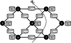
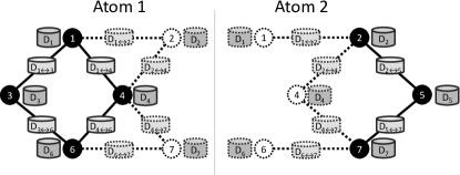
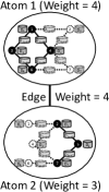
The graph is initially over-partitioned by an expert, or by using a graph partitioning heuristic (for instance Metis [35]) into parts where is much greater than the number of machines (see Fig. 4(a)). Each part is stored as a different file possibly on a distributed store (HDFS, Amazon S3). The connectivity structure of the parts is then represented as a meta-graph with vertices. Each vertex of the meta-graph represents a partition, and is weighted by the amount of data it stores. Each edge is weighted by the number of edges crossing the partitions.
Distributed loading is accomplished by performing a fast balanced partition of the meta-graph into parts ,and each machine constructs its local partition of the graph by merging its assigned files. To facilitate communication, each machine also stores the ghost of its local partition: the set of vertices and edges adjacent to the partition boundary (see Fig. 4(b)). The ghosts conveniently act as local caches for their true counterparts across the network, and cache coherence is managed using versioning [36].
The two-stage partitioning technique allows one graph partition to be reused for different numbers of machines without incurring a repartitioning step. A study on the quality of the two stage partitioning scheme is beyond the scope of this paper, though simple experiments using graphs obtained from [37] suggest that the performance is comparable to direct partitioning.
4.2 GraphLab Engines
The GraphLab engine emulates the execution model defined in Sec. 3.4 and is responsible for executing update task and sync operations, maintaining the update task set , and ensuring sequential consistency with respect to the appropriate consistency model (see Sec. 3.5). As discussed earlier in Sec. 3.4, variations in how is maintained and the order in which elements are removed is up to the implementation and can affect performance and expressiveness. To evaluate this trade-off we built the low-overhead Chromatic Engine, which executes in a fixed order, and the more expressive Locking Engine which executes in an asynchronous prioritized order.
4.2.1 Chromatic Engine
The Chromatic Engine imposes a static ordering on the update task set by executing update task in a canonical order (e.g., the order of their vertices). A classic technique [20] to achieve a sequentially consistent parallel execution of a set of dependent tasks is to construct a vertex coloring. A vertex coloring assigns a color to each vertex such that no adjacent vertices share the same color. Given a vertex color of the data graph, we can satisfy the edge consistency model by executing, in parallel, all update tasks with vertices of the same color before proceeding to the next color. The sync operation can be run safely between colors.
We can satisfy the other consistency models simply by changing how the vertices are colored. The stronger full consistency model is satisfied by constructing a second-order vertex coloring (i.e., no vertex shares the same color as any of its distance two neighbors). Conversely, we can trivially satisfy the vertex consistency model by assigning all vertices the same color.
In the distributed setting it is necessary to both prevent overlapping computation, and also synchronize any changes to ghost vertices or edge data between colors. A full communication barrier is enforced between color phases to ensure completion of all data synchronization before the next color begins. To maximize network throughput and to minimize time spent in the barrier, synchronization of modified data is constantly performed in the background while update functions are executing.
Approximate graph coloring can be quickly obtained through graph coloring heuristics. Furthermore, many ML problems have obvious colorings. For example, many optimization problems in ML are naturally expressed as bipartite graphs (Sec. 5), while problems based upon templated Bayesian Networks [30] can be easily colored by the expert through inspection of the template model [22].
The simple design of the Chromatic engine is made possible by the explicit communication structure defined by the data graph, allowing data to be pushed directly to the machines requiring the information. In addition, the cache versioning mechanism further optimizes communication by only transmitting modified data. The advantage of the Chromatic engine lies its predictable execution schedule. Repeated invocations of the chromatic engine will always produce identical update sequences, regardless of the number of machines used. This property makes the Chromatic engine highly suitable for testing and debugging purposes. We provide a distributed debugging tool which halts at the end of each color, allowing graph data and scheduler state to be queried.
4.2.2 Locking Engine
Even though the chromatic engine is a complete implementation of the GraphLab abstraction as defined in Sec. 3, it does not provide sufficient scheduling flexibility for many interesting applications. Here we describe an implementation which directly extends from a typical shared memory implementation to the distributed case.
In the shared memory implementation of GraphLab, the consistency models were implemented by associating a readers-writer lock with each vertex. The vertex consistency model is achieved by acquiring a write lock on the central vertex of each requested scope. The edge-consistency model is achieved by acquiring a write lock on the central vertex, and read locks on adjacent vertices. Finally, full consistency is achieved by acquiring write locks on the central vertex and all adjacent vertices.
The main execution loop in the shared memory setting uses worker threads to pull tasks from the scheduler, acquire the required locks, evaluate the task, and then release the locks. This loop is repeated until the scheduler is empty. The sync operation is triggered by a global shared-memory task counter. Periodically, as sync operations become ready, all threads are forced to synchronize in a barrier to execute the sync operation.
In the distributed setting, the same procedure is used. However, since the graph is partitioned, we restrict each machine to only run updates on vertices it owns. The ghost vertices/edges ensure that the update will always have direct memory access to all information in the scope, and distributed locks are used to ensure that the ghost is up to date. Finaly, the scheduling flexibility permitted by the abstraction allow the use of efficient approximate FIFO/priority task-queues. Distributed termination is evaluated using a multi-threaded variant of the distributed consensus algorithm described in [38].
Since the distributed locking and synchronization introduces substantial latency, we rely on several techniques to reduce latency and hide its effects [39]. First, the ghosting system provides caching capabilities eliminating the need to wait on data that has not changed remotely. Second, all locking requests and synchronization calls are pipelined allowing each thread to request multiple scope locks simultaneously and then evaluate the update tasks only when the locks are satisfied. The lock pipelining technique we implemented shares similarities to the continuation passing method in [40].
5 Applications
To evaluate the performance of the distributed GraphLab runtime as well as the representational capabilities of the GraphLab abstraction, we implemented several state-of-the-art ML algorithms. Each algorithm is derived from active research in machine learning and is applied to real world data sets with different structures (see Table 2), update functions, and sync operations. In addition, each application tests different features of the distributed GraphLab framework. The source and datasets for all the applications may be obtained from [http://graphlab.org].
| Exp. | #Verts | #Edges | Vertex Data | Edge Data | Update Complexity | Shape | Partition | Engine |
|---|---|---|---|---|---|---|---|---|
| Netflix | 0.5M | 99M | bipartite | random | Chromatic | |||
| CoSeg | 10.5M | 31M | 3D grid | frames | Locking | |||
| NER | 2M | 200M | bipartite | random | Chromatic |
5.1 Netflix Movie Recommendation
The Netflix movie recommendation task [41] uses collaborative filtering to predict the movie ratings of users, based on the ratings of similar users. The alternating least squares (ALS) algorithm is commonly used in collaborative filtering. The input to ALS is a sparse users by movies matrix containing the movie ratings of each user. The algorithm proceeds by computing a low rank approximate matrix factorization:
![[Uncaptioned image]](/html/1107.0922/assets/x8.png) |
where and are rank matrices. The ALS algorithm alternates between computing the least-squares approximation for or while holding the other fixed. The quality of the approximation depends on the magnitude of , as shown in Fig. 5(a).
While ALS may not seem like a graph algorithm, it can be represented elegantly using the GraphLab abstraction. The sparse matrix defines a bipartite graph (see Table 2) connecting each user with the movie he/she rated. The edge data contains the rating for a movie-user pair. The vertex data for users and movies contains the corresponding row in and column in respectively.
The ALS algorithm can be encoded as an update function that recomputes the least-squares solution for the current movie or user given the neighboring users or movies. Each local computation is accomplished using BLAS/LAPACK linear algebra library for efficient matrix operations. The bipartite graph is naturally two colored, thus the program is executed using the chromatic engine with two colors. A sync operation is used to compute the prediction error during the run. Due to the density of the graph, a random partitioning was used.
5.2 Video Cosegmentation (CoSeg)
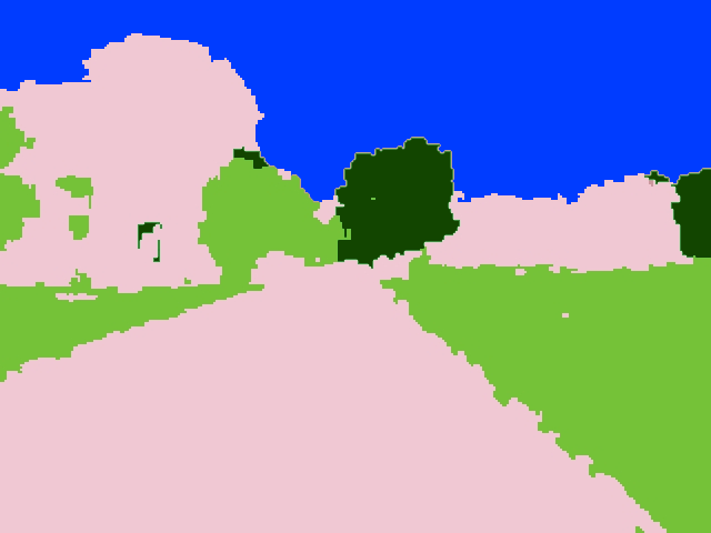
Video cosegmentation automatically identifies and clusters spatio-temporal segments of video (see Fig. 5(b)) that share similar texture and color characteristics. The resulting segmentation (see Fig. 5(c)) can be used in scene understanding and other computer vision and robotics applications. Previous cosegmentation methods [42] have focused on processing frames in isolation. As part of this work, we developed a joint cosegmentation algorithm that processes all frames simultaneously and therefore is able to model temporal stability.


Food Religion City onion Catholic Munich garlic Fremasonry Cape Twn. noodles Marxism Seoul blueberries Catholic Chr. Mexico Cty. beans Humanism Winnipeg
We preprocessed frames of high-resolution video by coarsening each frame to a regular grid of rectangular super-pixels. Each super-pixel stores the color and texture statistics for all the raw pixels in its domain. The CoSeg algorithm predicts the best label (e.g., sky, building, grass, pavement, trees) for each super pixel using Gaussian Mixture Model (GMM) [43] in conjunction with Loopy Belief Propagation (LBP) [31]. The GMM estimates the best label given the color and texture statistics in the super-pixel. The algorithm operates by connecting neighboring pixels in time and space into a large three-dimensional grid and uses LBP to smooth the local estimates. We combined the two algorithms so that CoSeg alternates between LBP to compute the label for each super-pixel given the current GMM and then updating the GMM given the labels from LBP.
The GraphLab data graph structure for video cosegmentation is the three dimensional grid graph (see Table 2). The vertex data stores the current label distribution as well as the color and texture statistics for each super-pixel. The edge data stores the parameters needed for the LBP algorithm. The parameters for the GMM are maintained using the sync operation. The GraphLab update function executes the LBP local iterative update. We implement the state-of-the-art adaptive update schedule described by [27], where updates which are expected to change vertex values significantly are prioritized. We therefore make use of the locking engine with the approximate priority ordering task queue. Furthermore, the graph has a natural partitioning by slicing across frames. This also allows feature processing of the video to be performed in an embarrassingly parallel fashion, permitting the use of Hadoop for preprocessing.
5.3 Named Entity Recognition (NER)
Named Entity Recognition (NER) is the task of determining the type (e.g., Person, Place, or Thing) of a noun-phrase (e.g., Obama, Chicago, or Car) from its context (e.g., “President __ …”, “…lives near __.”, or “…bought a __.”). NER is used in many natural language processing applications as well as information retrieval. In this application we obtained a large crawl of the web and we counted the number of occurrences of each noun-phrase in each context. Starting with a small seed set of pre-labeled noun-phrases, the CoEM algorithm [44] labels the remaining noun-phrases and contexts (see Table 5(d)) by alternating between estimating the best assignment to each noun-phrase given the types of its contexts and estimating the type of each context given the types of its noun-phrases.
The GraphLab data graph for the NER problem is bipartite with vertices corresponding to each noun-phrase on one side and vertices corresponding to each context on the other. There is an edge between a noun-phrase and a context if the noun-phrase occurs in the context. The vertex for both noun-phrases and contexts stores the estimated distribution over types. The edge stores the number of times the noun-phrase appears in that context.
The NER computation is represented in a simple GraphLab update function which computes a weighted sum of probability tables stored on adjacent vertices and then normalizes. Once again, the bipartite graph is naturally two colored, allowing us to use the chromatic scheduler. Due to the density of the graph, a random partitioning was used. Since the NER computation is relatively light weight and uses only simple floating point arithmetic; combined with the use of a random partitioning, this application stresses the overhead of the GraphLab runtime as well as the network.
5.4 Other Applications
In the course of our research, we have also implemented several other algorithms, which we describe briefly:
Gibbs Sampling on a Markov Random Field. The task is to compute a probability distribution for a graph of random variables by sampling. Algorithm proceeds by sampling a new value for each variable in turn conditioned on the assignments of the neighboring variables. Strict sequential consistency is necessary to preserve statistical properties [22].
Bayesian Probabilistic Tensor Factorization (BPTF). This is a probabilistic Markov-Chain Monte Carlo version of Alternative Least Squares that also incorporates time-factor into the prediction. In this case, the tensor is decomposed into three matrices which can be represented in GraphLab as a tripartite graph.
In addition, GraphLab has been used successfully in several other research projects like clustering communities in the twitter network, collaborative filtering for BBC TV data as well as non-parametric Bayesian inference.
6 Evaluation
We evaluated GraphLab on the three applications (Netflix, CoSeg and NER) described above using important large-scale real-world problems (see Table 2). We used the Chromatic engine for the Netflix and NER problems and the Locking Engine for the CoSeg application. Equivalent Hadoop and MPI implementations were also tested for both the Netflix and the NER application. An MPI implementation of the asynchronous prioritized LBP algorithm needed for CoSeg requires building an entirely new asynchronous sequentially consistent system and is beyond the scope of this work.
Experiments were performed on Amazon’s Elastic Computing Cloud (EC2) using up to 64 High-Performance Cluster (HPC) instances (cc1.4xlarge). The HPC instances (as of February 2011) have 2 x Intel Xeon X5570 quad-core Nehalem architecture with 22 GB of memory, connected by a low latency 10 GigaBit Ethernet network. All our timings include data loading time and are averaged over three or more runs. Our principal findings are:
-
GraphLab is fast! On equivalent tasks, GraphLab outperforms Hadoop by 20x-60x and is as fast as custom-tailored MPI implementations.
-
GraphLab’s performance scaling improves with higher computation to communication ratios. When communication requirements are high, GraphLab can saturate the network, limiting scalability.
-
The GraphLab abstraction more compactly expresses the Netflix, NER and Coseg algorithms than MapReduce or MPI.
6.1 Scaling Performance
In Fig. 6(a) we present the parallel speedup of GraphLab when run on 4 to 64 HPC nodes. Speedup is measured relative to the 4 HPC node running time. On each node, GraphLab spawned eight shared memory engine threads (matching the number of cores). Of the three applications, CoSeg demonstrated the best parallel speedup, achieving nearly ideal scaling up to 32 nodes and moderate scaling up to 64 nodes. The excellent scaling of the CoSeg application can be attributed to its sparse data graph (maximum degree 6) and a computationally intensive update function. While Netflix demonstrated reasonable scaling up to 16 nodes, NER achieved only modest 3x improvement beyond 16x or more nodes.
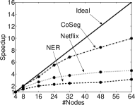
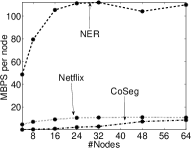
We attribute the poor scaling performance of NER to the large vertex data size (816 bytes), dense connectivity, and poor partitioning (random cut) which resulted in substantial communication overhead per iteration. Fig. 6(b) shows for each application, the average number of bytes transmitted by each node per second as the cluster size is increased. Beyond 16 nodes, it is evident that NER saturates the network, with each machine sending at a rate of over 100MB per second. Note that Fig. 6(b) plots the average transmission rate and the peak rate could be significantly higher.
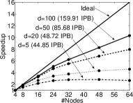
To better understand the effect of the ratio between computation and communication on the scaling of the GraphLab abstraction, we varied the computational complexity of the Netflix experiment. The amount of computation performed in Netflix can be controlled by varying : the dimensionality of the approximating matrices in Eq. (5.1). In Fig. 6(c) we plot the speedup achieved for varying values of and the corresponding number of instructions per byte (IPB) of data accessed. The speedup at 64 nodes increases quickly with increasing IPB indicating that speedup is strongly coupled.
6.2 Comparison to Other Frameworks
In this section, we compare our GraphLab implementation of the Netflix application and the NER application to an algorithmically equivalent Hadoop and MPI implementations.
MapReduce/Hadoop. We chose to compare against Hadoop, due to its wide acceptance in the Machine Learning community for large scale computation (for example the Mahout project [2, 45]). Fair comparison is difficult since Hadoop is implemented in Java while ours is highly optimized C++. Additionally, to enable fault tolerance, Hadoop stores interim results to disk. In our experiments, to maximize Hadoop’s performance, we reduced the Hadoop Distributed Filesystem’s (HDFS) replication factor to one, eliminating fault tolerance. A significant amount of our effort was spent tuning the Hadoop job parameters to improve performance.
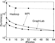
Fig. 6(d) shows the running time for one iteration of Netflix application on GraphLab, Hadoop and MPI ( for all cases), using between 4 and 64 nodes. The Hadoop evaluation makes use of the of Sebastian Schelter contribution to the Mahout project333https://issues.apache.org/jira/browse/MAHOUT-542, while the MPI implementation was written from scratch. We find that GraphLab performs the same computation between 40x-60x times faster than Hadoop.
Fig. 7(a) plots the running for one iteration of the NER application on GraphLab, Hadoop and MPI. The Hadoop implementation was aggressively optimized: we implemented specialized binary marshaling methods which improve performance by 5x over a baseline implementation. Fig. 7(a) shows that the GraphLab implementation of NER obtains a 20-30x speedup over Hadoop.
Part of the performance of GraphLab over Hadoop can be explained by implementation differences, but it is also easy to see that the GraphLab representation of both NER and ALS is inherently more efficient. For instance the case of NER, when implemented in Hadoop, the Map-function, normally the cornerstone of embarrassing-parallelism in MapReduce essentially does no work. The Map only serves to emit the vertex probability table for every edge in the graph, which corresponds to over 100 gigabytes of HDFS writes occurring between the Map and Reduce stage. The cost of this operation can easily be multiplied by factor of three if HDFS replication is turned on. Comparatively, the GraphLab update function is simpler as users do not need to explicitly define the flow of information from the Map to the Reduce, but simply modifies data in-place. In the case of such iterative computation, GraphLab’s knowledge of the dependency structure allow modified data to be communicated directly to the destination.
Overall, we can attribute GraphLab’s superior performance over Hadoop to the fact that the abstraction is a much better fit. It presents a simpler API to the programmer and through the data graph, and informs GraphLab about the communication needs of the program.
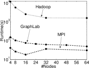
MPI. In order to analyze the cost of using a higher level abstraction we implemented efficient versions of the Netflix and NER applications using MPI. The implementations made use of synchronous MPI collective operations for communication. The final performance results can be seen in Fig. 6(d) and Fig. 7(a). We observe that the performance of MPI and GraphLab implementations are similar and conclude that GraphLab does not impose significant performance penalty. GraphLab also has the advantage of being a higher level abstraction and is easier to work with.
6.3 Locking Engine Evaluation
The CoSeg application makes use of dynamic prioritized scheduling which requires the locking engine (Sec. 4.2.2). To the best of our knowledge, there are no other abstractions which provide the dynamic asynchronous scheduling as well as the sequentially consistent sync (reduction) capabilities required by this application.
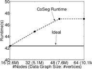
In Fig. 6(a) we demonstrate that the locking engine can provide significant scalability and performance on the large 10.5 million vertex graph used by this application, achieving a 10x speedup with 16x more machines. We also observe from Fig. 8(a) that the locking engine provides nearly optimal weak scalability. The runtime does not increase significantly as the size of the graph increases proportionately with the number of processors. We can attributed this to the properties of the graph partition where the number of edges crossing machines increases linearly with the number of processors, resulting in low communication volume.
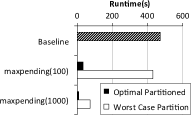
In Fig. 8(b) we further investigate the properties of the distributed lock implementation described in Sec. 4.2.2. The evaluation is performed on a tiny 32-frame (192K vertices) problem on a 4 node cluster. Two methods of cutting the graph is explored. The first method is an “optimal partition” where the frames are distributed evenly in 8 frame blocks to each machine. The second method is a “worst case partition” where the frames are striped across the machines; this is designed to stress the distributed lock implementation since every scope acquisition is forced to acquire a remote lock. The maximum number of lock requests allowed in the pipeline is varied (maxpending). The baseline evaluation is optimal partitioning with the maxpending set to zero.
Fig. 8(b) demonstrates that on well-partitioned models, increasing the maximum number of pending locks from to increases performance significantly. However, we observe diminishing returns as maxpending is further increased to . On the other hand when the partitioning is poor, increasing the number of pending locks to improves performance significantly.
6.4 EC2 Cost evaluation
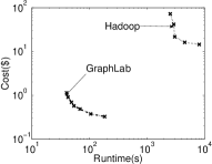
To help put costs in perspective, we plot a price-performance curve for the Netflix application in Fig. 8(c). The curve shows the cost one should expect to pay to obtain a certain desired performance level. To ensure interpretability of the curve, the cost assumes fine-grained billing even though Amazon EC2 billing rounds up utilization time to the nearest hour. The curve has an “L” shape implying diminishing returns: as lower runtimes are desired, the cost of attaining those runtimes increases faster than linearly. As a comparison, we also provide the price-performance curve for Hadoop on the same application. It is evident that for the Netflix application, GraphLab is about two orders of magnitude more cost-effective than Hadoop.
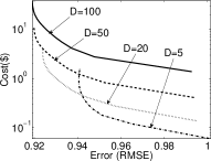
Fig. 8(d) is an interesting plot which the cost required to attain a certain degree of accuracy (lower RMSE is better) on the Netflix task using 32 HPC nodes. Similarly the curve demonstrates diminishing returns: the cost of achieving lower test errors increase quickly. The lower bound of all four curves inform the reader with the “cheapest” value of which attains the desired accuracy.
7 Related Work
Perhaps the closest approach to our abstraction is Pregel [8], which also computes on a user-defined data graph. The most important difference is that Pregel is based on the BSP model [10], while we propose an asynchronous model of computation. Parallel BGL [9] is similar.
Piccolo [11] shares many similarities to GraphLab on an implementation level, but does not explicitly model data dependencies. Sequential consistency of execution is also not guaranteed.
MapReduce [1] and Dryad [3] are popular distributed data-flow frameworks which are used extensively in data mining. The use of MapReduce for ML in multi-core setting was first made popular by Chu et. al. [2] in 2006. Such data-flow models cannot express efficiently sparse dependencies or iterative local computation. There are several extensions to these frameworks, such as MapReduce Online [13], Twister [23], Nexus [14] and Spark [15], but none present a model which supports sparse dependencies with asynchronous local computation. Most notably, Surfer [46] extends MapReduce with a special primitive propagation for edge-oriented tasks in graph processing, but this primitive is still insufficient for asynchronous local computation.
Recently, work by Pearce et. al [12] proposed a system for asynchronous multithreaded graph traversals, including support for prioritized ordering. However, their work does does not address sequential consistency or the distributed setting.
Finally, OptiML [25], a parallel programming language, for Machine Learning. We share their approach of developing domain specific parallel solutions. OptiML parallelizes operations on linear algebra data structures, while GraphLab defines a higher level model of parallel computation.
8 Conclusion and Future Work
Many important ML techniques utilize sparse computational dependencies, are iterative, and benefit from asynchronous computation. Furthermore, sequential consistency is an important requirement which ensures statistical correctness and guarantees convergence for many ML algorithms. Finally, prioritized ordering of computation can greatly accelerate performance.
The GraphLab abstraction we proposed allows the user to explicitly represent structured dependent computation and extracts the available parallelism without sacrificing sequential consistency. Furthermore, GraphLab’s sync operation allows global information to be efficiently aggregated even as an asynchronous iterative algorithm proceeds. Since the graph representation of computation is a natural fit for many ML problems, GraphLab simplifies the design, implementation, and debugging of ML algorithms.
We developed a highly optimized C++ distributed implementation of GraphLab and evaluated it on three state-of-the-art ML algorithms using real data: collaborative filtering on the Netflix dataset, Named Entity Recognition, and Video Cosegmentation. The evaluation was performed on Amazon EC2 using up to 512 processors in 64 HPC nodes. We demonstrated that GraphLab outperforms Hadoop (a popular framework in the ML community) by 20-60x, and is competitive with tailored MPI implementations.
Future work includes supporting dynamic and implicitly represented graphs, as well as support for graphs in external storage. The current implementation provides limited support for external storage through the use of mmaped memory for vertex and edge data. There are interesting possibilities for the intelligent placement and caching of graph data to maximize performance [12].
While the current GraphLab implementation does not provide fault tolerance, relatively simple modifications could be made to support snapshotting capabilities. In particular, a globally consistent snapshot mechanism can be easily performed using the Sync operation. Additionally, we plan to extend GraphLab to other architectures including GPUs and supercomputers.
References
- [1] J. Dean and S. Ghemawat. MapReduce: simplified data processing on large clusters. Commun. ACM, 51(1):107–113, 2008.
- [2] C. T. Chu, S. K. Kim, Y. A. Lin, Y. Yu, G. R. Bradski, A. Y. Ng, and K. Olukotun. Map-Reduce for machine learning on multicore. In NIPS, pages 281–288. MIT Press, 2006.
- [3] M. Isard, M. Budiu, Y. Yu, A. Birrell, and D. Fetterly. Dryad: distributed data-parallel programs from sequential building blocks. ACM SIGOPS Operating Systems Review, 41(3):59–72, 2007.
- [4] L. Dagum and R. Menon. OpenMP: an industry standard API for shared-memory programming. Computational Science & Engineering, IEEE, 5(1):46–55, 1998.
- [5] W. Gropp, E. Lusk, N. Doss, and A. Skjellum. A high-performance, portable implementation of the MPI message passing interface standard. Parallel Computing, 22(6):789–828, 1996.
- [6] K. Asanovic, R. Bodik, B.C. Catanzaro, J.J. Gebis, P. Husbands, K. Keutzer, D.A. Patterson, W.L. Plishker, J. Shalf, S.W. Williams, et al. The landscape of parallel computing research: A view from berkeley. EECS Department, University of California, Berkeley, Tech. Rep. UCB/EECS-2006-183, 2006.
- [7] Y. Low, J. Gonzalez, A. Kyrola, D. Bickson, C. Guestrin, and J. M. Hellerstein. Graphlab: A new parallel framework for machine learning. In UAI, July 2010.
- [8] G. Malewicz, M. H. Austern, A. J. C. Bik, J. C. Dehnert, I. Horn, N. Leiser, and G. Czajkowski. Pregel: a system for large-scale graph processing. In PODC ’09, page 6. ACM, 2009.
- [9] D. Gregor and A. Lumsdaine. The parallel BGL: A generic library for distributed graph computations. POOSC, 2005.
- [10] L.G. Valiant. A bridging model for parallel computation. Communications of the ACM, 33(8):103–111, 1990.
- [11] R. Power and J. Li. Piccolo: building fast, distributed programs with partitioned tables. In OSDI ’10, pages 1–14, 2010.
- [12] R. Pearce, M. Gokhale, and N.M. Amato. Multithreaded Asynchronous Graph Traversal for In-Memory and Semi-External Memory. In SuperComputing ’10, pages 1–11, 2010.
- [13] T. Condie, N. Conway, P. Alvaro, J. M. Hellerstein, K. Elmeleegy, and R. Sears. Mapreduce online. In NSDI’10, pages 21–21, 2010.
- [14] B. Hindman, A. Konwinski, M. Zaharia, and I. Stoica. A common substrate for cluster computing. In HotCloud, pages 19–19, 2009.
- [15] M. Zaharia, M. Chowdhury, M.J. Franklin, S. Shenker, and I. Stoica. Spark: cluster computing with working sets. In HotCloud ’10. USENIX Association, 2010.
- [16] J. E. Gonzalez, Y. Low, C. Guestrin, and D. O’Hallaron. Distributed parallel inference on large factor graphs. In UAI, 2009.
- [17] J. Choi, J. Dongarra, S. Ostrouchov, A. Petitet, D. Walker, and R. Whaley. A proposal for a set of parallel basic linear algebra subprograms. PARA, 1996.
- [18] C.E. Leiserson. The Cilk++ concurrency platform. In DAC. IEEE, 2009.
- [19] J. Gonzalez, Y. Low, and C. Guestrin. Residual splash for optimally parallelizing belief propagation. In AISTATS, 2009.
- [20] D. P. Bertsekas and J. N. Tsitsiklis. Parallel and distributed computation: numerical methods. Prentice-Hall, Inc., USA, 1989.
- [21] W. G. Macready, A. G. Siapas, and S. A. Kauffman. Criticality and parallelism in combinatorial optimization. Science, 271:271–56, 1995.
- [22] J. Gonzalez, Y. Low, A. Gretton, and C. Guestrin. Parallel gibbs sampling: From colored fields to thin junction trees. In AISTATS, 2011.
- [23] J. Ekanayake, H. Li, B. Zhang, T. Gunarathne, S.H. Bae, J. Qiu, and G. Fox. Twister: A runtime for iterative MapReduce. In HPDC. ACM, 2010.
- [24] M. Jiayuan, S. Chakradhar, and A. Raghunathan. Best-effort parallel execution framework for recognition and mining applications. In IPDPS, pages 1 –12, May 2009.
- [25] H. Chafi, A. K. Sujeeth, K. J. Brown, H. Lee, A. R. Atreya, and K. Olukotun. A domain-specific approach to heterogeneous parallelism. In PPoPP ’11, pages 35–46. ACM, 2011.
- [26] S. Geman and D. Geman. Stochastic relaxation, Gibbs distributions, and the bayesian restoration of images. In PAMI, 1984.
- [27] G. Elidan, I. McGraw, and D. Koller. Residual Belief Propagation: Informed scheduling for asynchronous message passing. In UAI ’06, pages 165–173, 2006.
- [28] B Efron, T Hastie, I M Johnstone, and Robert Tibshirani. Least angle regression. Annals of Statistics, 32:407–451, 2004.
- [29] L. Page, S. Brin, R. Motwani, and T. Winograd. The pagerank citation ranking: Bringing order to the web. Technical Report 1999-66, Stanford InfoLab, November 1999.
- [30] D Koller and N Friedman. Probabilistic Graphical Models: Principles and Techniques. MIT Press, 2009.
- [31] J. Pearl. Probabilistic reasoning in intelligent systems: networks of plausible inference. Morgan Kaufmann, 1988.
- [32] T. P. Minka. A family of algorithms for approximate bayesian inference. PhD thesis, MIT, 2001. AAI0803033.
- [33] E. P. Xing, M. I. Jordan, and S. Russell. A Generalized Mean Field Algorithm for Variational Inference in Exponential Families. In UAI ’03, pages 583–559, 2003.
- [34] L Lamport. How to Make a Multiprocessor Computer That Correctly Executes Multiprocess Programs. IEEE Trans. Comput., C-28(9):690–691, 1979.
- [35] G. Karypis and V. Kumar. Multilevel k-way partitioning scheme for irregular graphs. J. Parallel Distrib. Comput., 48(1):96–129, 1998.
- [36] P.A. Bernstein and N. Goodman. Concurrency control in distributed database systems. ACM Comput. Surv., 1981.
- [37] J. Leskovec. Stanford large network dataset collection, 2011.
- [38] J. Misra. Detecting termination of distributed computations using markers. In SIGOPS, 1983.
- [39] A. Gupta, J. Hennessy, K. Gharachorloo, T. Mowry, and W.-D. Weber. Comparative evaluation of latency reducing and tolerating techniques. In Computer Architectures, pages 254 – 263, 1991.
- [40] John Turek, Dennis Shasha, and Sundeep Prakash. Locking without blocking: making lock based concurrent data structure algorithms nonblocking. In PODS ’92, pages 212–222. ACM, 1992.
- [41] Yunhong Zhou, Dennis Wilkinson, Robert Schreiber, and Rong Pan. Large-scale parallel collaborative filtering for the netflix prize. In LECT NOTES COMPUT SC, 2008.
- [42] D. Batra, A. Kowdle, D. Parikh, L. Jiebo, and C. Tsuhan. iCoseg: Interactive co-segmentation with intelligent scribble guidance. In CVPR, pages 3169 –3176, 2010.
- [43] C. M. Bishop. Pattern Recognition and Machine Learning (Information Science and Statistics). Springer-Verlag, Secaucus, NJ, USA, 2006.
- [44] R. Jones. Learning to Extract Entities from Labeled and Unlabeled Text. PhD thesis, Carnegie Mellon University, School of Computer Science, Pittsburgh, Pennsylvania, 2005.
- [45] U. Kang, C. E. Tsourakakis, and C. Faloutsos. Pegasus: A peta-scale graph mining system implementation and observations. In ICDM ’09. IEEE Computer Society, 2009.
- [46] R. Chen, X. Weng, B. He, and M. Yang. Large graph processing in the cloud. In ICMD ’10, pages 1123–1126. ACM, 2010.