Edge-based compartmental modeling for epidemic spread Part II: Model Selection and Hierarchies

Joel C. Miller111Center for Communicable Disease Dynamics, Department of Epidemiology, Harvard School of Public Health 222Fogarty International Center, NIH    Erik M. Volz333Department of Epidemiology, University of Michigan, Ann Arbor
Abstract

We consider the edge-based compartmental models for epidemic spread developed in [5]. We show conditions under which simpler models may be substituted for more detailed models, and in so doing we define a hierarchy of epidemic models. In particular we provide conditions under which it is appropriate to use the standard mass action SIR model, and we show what happens when these conditions fail. Using our hierarchy, we provide a procedure leading to the choice of the appropriate model for a given population. Our result about the convergence of models to the Mass Action model gives clear, rigorous conditions under which the Mass Action model is accurate.

1 Introduction

The spread of epidemics through populations is affected by many factors such as the infectiousness of the disease, the duration of infection, the distribution of contacts through the population, and the typical duration of contacts. Typically for predicting epidemic spread or intervention effectiveness, we want an accurate, but simple, model that captures the relevant effects.

In our earlier work [5], we introduced the edge-based compartmental modeling approach for the spread of SIR diseases in populations with different contact dynamics. In particular we showed that edge-based compartmental models can capture contact duration and social heterogeneity (variation in contact levels) simultaneously in mathematically and conceptually simple terms. The models we studied all assumed that the population was made up of individuals who were identical except for their contact levels. We modeled the population as a network, with nodes representing individuals joined by edges representing potentially transmitting contacts. We also assumed a simple disease, with transmission occuring at rate β𝛽\beta per edge and recovery occuring at rate γ𝛾\gamma. In this paper we investigate the relationships between models and how to choose the simplest model appropriate for a given population.

The models discussed in [5] can each be classified by two features: the first is how contact duration is determined and the second is how contact levels are distributed through the population. Table 1 summarizes the models and their underlying assumptions.

The contact duration falls into three possibilities: it can be permanent, finite, or fleeting. In the permanent case, a contact that exists at any time has always existed and will always exist. In the finite case contacts may change over time. In the fleeting case, contacts are so brief that over any macroscopic time scale an individual samples a very large number of neighbors, and so it is safe to assume that the total contact time with infected individuals matches its expected value.

The distribution of contact levels can be split into two types. In one set of models (expected degree models), we assign an expected degree κ𝜅\kappa to a node. The probability that an edge exists between two nodes is proportional to the expected degrees of each node. Edges are created independently of one another, so the existence of an edge between u𝑢u and v𝑣v does not alter whether an edge can exist between u𝑢u and w𝑤w. Note that the expected degree can take any non-negative real value, and we assume that the distribution of κ𝜅\kappa is given by the probability density function ρ(κ)𝜌𝜅\rho(\kappa). In the other set of models (actual degree models) we assign an actual integer number of contacts k𝑘k, the degree, to each individual though in the case of the dormant contact model not all of these contacts must be active at all times. We think of an individual as having k𝑘k stubs (or half-edges) which pair randomly with stubs of other nodes to form edges. In this case the existence of an edge between u𝑢u and v𝑣v removes an available stub from u𝑢u, and so it affects the probability of an edge between u𝑢u and w𝑤w. The distribution of degrees is given by the probability mass function P(k)𝑃𝑘P(k).

The distinction between the expected degree models and the actual degree models becomes apparent when we calculate the probability that an individual is susceptible. For the expected degree models, there is a continuum of risk levels and so we will have to calculate the per-expected degree probability of not having been infected. In contrast for the actual degree models the risk is discretized. The calculation is slightly different in each case, but the underlying concepts are the same.

Model Contact Duration Heterogeneity type
Configuration Model (CM) Permanent Actual degree k𝑘k
Mixed Poisson (MP) Permanent Expected degree κ𝜅\kappa
Dynamic Variable-Degree (DVD) Finite Expected degree κ𝜅\kappa
Dynamic Fixed-Degree (DFD) Finite Actual degree k𝑘k
Mean Field Social Heterogeneity (MFSH) Fleeting Contact rate k𝑘k or κ𝜅\kappa
Dormant Contact (DC) Finite active and dormant Maximum degree kmsubscript𝑘𝑚k_{m}
Mass Action (MA) Fleeting None
Table 1: The basic models and their underlying assumptions. Contacts are assumed to form and break at some rate which can vary from zero (permanent) to infinite (fleeting). Depending on the process governing contact formation, we may know the actual degree k𝑘k of an individual or we may know its expected degree.

The equations produced by edge-based compartmental models are surprisingly simple. Nevertheless the cases with simpler assumptions lead to simpler equations, and so it is worth knowing what conditions allow the use of a simpler model. In general when contact duration is short compared to the infection and recovery time scales it is safe to use the fleeting contact models, while if contact duration is long compared to the duration of the epidemic it is safe to use the permanent contact models. However, there are some less obvious limits. If the average degree Kdelimited-⟨⟩𝐾\left\langle K\right\rangle is large while the rate of transmission per edge scales such that β𝛽\beta is of order 1/K1delimited-⟨⟩𝐾1/\left\langle K\right\rangle and the recovery rate γ𝛾\gamma is fixed, then the probability that any given edge transmits even once is small. The probability it transmits twice is negligible: the disease “sees” an edge at most once, so whether it is permanent, fleeting, or finite has no impact on disease spread. Thus we may treat the model as if the contacts are fleeting, which simplifies the equations. If further the contact distribution is such that the contact levels are generally close to the mean, then we can neglect variation in contact levels, and turn to the simple mass action model of [2, 1]. The precise condition required for this is somewhat technical: we must have |K4K4|/K41much-less-thandelimited-⟨⟩superscript𝐾4superscriptdelimited-⟨⟩𝐾4superscriptdelimited-⟨⟩𝐾41|\left\langle K^{4}\right\rangle-\left\langle K\right\rangle^{4}|/\left\langle K\right\rangle^{4}\ll 1 and K1much-greater-thandelimited-⟨⟩𝐾1\left\langle K\right\rangle\gg 1 with β^=βK^𝛽𝛽delimited-⟨⟩𝐾\hat{\beta}=\beta\left\langle K\right\rangle fixed. When this does not hold, there can be a significant deviation away from the mass action model.

In this paper we begin by providing a flow chart leading to selection of the appropriate model for a given population. Following the flow chart, we introduce the hierarchy of the models which underlies the flow chart. We describe the precise assumptions of the models and demonstrate some of the simpler parts of the hierarchy. After that, we consider some of the more difficult aspects of the hierarchy. We finally discuss some of the implications and limitations of our approach. In particular, we note that we give a simple heuristic for when the Mass Action equations are appropriate. In the Appendix we provide more rigorous justifications for the claims in the hierarchy section. Because of its importance, we include the rigorous proof of conditions under which the Mass Action equations hold in the main text.

2 Model Selection

START Q1 Q2 Q3 Q4 Q5 Q6 MA MFSH MP CM DFD DVD DC YesNoYesNoNoYesActualExpectedYesNoYesNo
  • Q1: Is the average degree Kdelimited-⟨⟩𝐾\left\langle K\right\rangle large and does the probability that an infected node recovers before transmitting scale like 1/K1delimited-⟨⟩𝐾1/\left\langle K\right\rangle?
    or
    Is an existing edge from an infected neighbor much more likely to be deleted than to have infection transmit?

  • Q2: Do almost all contacts stay the same during the time scale of the epidemic?

  • Q3: Is |K4K4|/K41much-less-thandelimited-⟨⟩superscript𝐾4superscriptdelimited-⟨⟩𝐾4superscriptdelimited-⟨⟩𝐾41|\left\langle K^{4}\right\rangle-\left\langle K\right\rangle^{4}|/\left\langle K\right\rangle^{4}\ll 1 where K4delimited-⟨⟩superscript𝐾4\left\langle K^{4}\right\rangle is the average fourth power of the degree and Kdelimited-⟨⟩𝐾\left\langle K\right\rangle is the average degree?

  • Q4: Can we measure the actual number of contacts an individual has, or just the expected number?

  • Q5: Does a new contact only form when an existing contact breaks?

  • Q6: For a given individual, are new contacts created at a constant rate regardless of the existing number of contacts?

Figure 1: Flow chart for model choice. Depending on the how the edge turnover rates compare to the infection and recovery rates, as well as the degree distribution, we arrive at different models. The model abbreviations are as in Table 1. This flow chart assumes that all structure in the population is due to heterogeneity in contact levels.

In Figure 1 we present a flow chart that can be used to select the appropriate model for a given population. The conditions depend on the degree distribution and the rate at which edges change. These are relatively straightforward to measure for a population [9, 13, 11]. From the observations of population and disease parameters, we can choose the simplest model to accurately represent disease spread in a given population. The equations for each model are described in Section 3.

Most existing modeling of infectious disease spread are based on the Mass Action model [2]. This flow chart gives appropriate conditions under which this model is reasonable. In general, we must have most degrees close to the average degree, but at the same time either contacts must have high turnover or the probability of transmission per contact is very low. Under these conditions, it is appropriate to use the MA model.

Before using this flow chart it is always prudent to be sure that the population does not violate other assumptions of the models. For example, different contact structure between age groups may require more consideration. If there are important features not captured by these models it may be possible to develop a custom model that captures the relevant detail (see [6, 12]). Otherwise we may not be able to rely on edge-based compartmental models and may have to use simulation.

The questions asked are somewhat vague in the sense that whether a number is large or not is somewhat a matter of opinion. In Section 3 we address this in more detail. We show how the results of the models converge as the parameter values change.

3 The model hierarchy

In this section we investigate the hierarchy of Figure 2 underlying the flow chart in Figure 1. We first give a brief overview of the standard simple model, the Mass Action model. We then consider the hierarchy of models. We find it convenient to consider the expected degree models before the actual degree models. We consider the models roughly in order of increasing complexity, explaining the underlying assumptions and giving the equations from [5]. If we can reduce the model to another model, we explain why this should happen and give some details of the mathematical explanation. More complete derivations are in the Appendix.

The Mean Field Social Heterogeneity models require further attention. We have two formulations, one in terms of expected degree κ𝜅\kappa and the other in terms of actual degree k𝑘k. We will not address this initially while we discuss the main structure of the hierarchy, but at the end of this section we show that the two formulations are mathematically equivalent in the sense that each can be derived from the other. So we do not distinguish between the two models in the hierarchy of Figure 2. We will also show that all other models reduce to Mean Field Social Heterogeneity in the large Kdelimited-⟨⟩𝐾\left\langle K\right\rangle limit if βK𝛽delimited-⟨⟩𝐾\beta\left\langle K\right\rangle and γ𝛾\gamma are both constant. In turn we have conditions under which the Mean Field Social Heterogeneity model reduces to the Mass Action model. Given any model with βK𝛽delimited-⟨⟩𝐾\beta\left\langle K\right\rangle and γ𝛾\gamma fixed, Kdelimited-⟨⟩𝐾\left\langle K\right\rangle\to\infty and K4/K41delimited-⟨⟩superscript𝐾4superscriptdelimited-⟨⟩𝐾41\left\langle K^{4}\right\rangle/\left\langle K\right\rangle^{4}\to 1, we arrive at the Mass Action model444It is worth noting that in the expected degree formulations the average fourth power of the degree and the average fourth power of the expected degrees are not equal, but if the ratio with K4superscriptdelimited-⟨⟩𝐾4\left\langle K\right\rangle^{4} tends to 111 for either, it does for the other as well..

Dormant contacts Dynamic Fixed-Degree Dynamic Variable-Degree Configuration Model Mixed Poisson Mean Field Social Heterogeneity Mass Action η1/βsubscript𝜂1𝛽\eta_{1}/\beta\to\infty, η2/η1subscript𝜂2subscript𝜂1\eta_{2}/\eta_{1} constant η2/η10subscript𝜂2subscript𝜂10\eta_{2}/\eta_{1}\to 0 P(km)=η1kmη2η1(km+1)η2ρ(κ)dκ𝑃subscript𝑘𝑚superscriptsubscriptsubscript𝜂1subscript𝑘𝑚subscript𝜂2subscript𝜂1subscript𝑘𝑚1subscript𝜂2𝜌𝜅differential-d𝜅P(k_{m})=\int_{\frac{\eta_{1}k_{m}}{\eta_{2}}}^{\frac{\eta_{1}(k_{m}+1)}{\eta_{2}}}\rho(\kappa)\,\mathrm{d}\kappa, η2/η1subscript𝜂2subscript𝜂1\eta_{2}/\eta_{1}\to\infty ηt0𝜂𝑡0\eta t\to 0ηt0𝜂𝑡0\eta t\to 0P(k)=0eκκkk!ρ(κ)dκ𝑃𝑘superscriptsubscript0superscript𝑒𝜅superscript𝜅𝑘𝑘𝜌𝜅differential-d𝜅P(k)=\int_{0}^{\infty}\frac{e^{-\kappa}\kappa^{k}}{k!}\rho(\kappa)\,\mathrm{d}\kappaη/β𝜂𝛽\eta/\beta\to\inftyη/β𝜂𝛽\eta/\beta\to\infty No contact rate variation Kdelimited-⟨⟩𝐾\left\langle K\right\rangle\to\infty, βK𝛽delimited-⟨⟩𝐾\beta\left\langle K\right\rangle constant Kdelimited-⟨⟩𝐾\left\langle K\right\rangle\to\infty, βK𝛽delimited-⟨⟩𝐾\beta\left\langle K\right\rangle constant Kdelimited-⟨⟩𝐾\left\langle K\right\rangle\to\infty, βK𝛽delimited-⟨⟩𝐾\beta\left\langle K\right\rangle constant Kdelimited-⟨⟩𝐾\left\langle K\right\rangle\to\infty, βK𝛽delimited-⟨⟩𝐾\beta\left\langle K\right\rangle constant Kdelimited-⟨⟩𝐾\left\langle K\right\rangle\to\infty, βK𝛽delimited-⟨⟩𝐾\beta\left\langle K\right\rangle constant K4K41delimited-⟨⟩superscript𝐾4superscriptdelimited-⟨⟩𝐾41\frac{\left\langle K^{4}\right\rangle}{\left\langle K\right\rangle^{4}}\to 1, βK𝛽delimited-⟨⟩𝐾\beta\left\langle K\right\rangle constant
Figure 2: The hierarchy structure. The edges summarize the relations between the models. A solid arrow from one model to another represents that the target model can be derived as a limiting case of the base model. We give heuristic explanations in the text for these and more rigorous derivations in the Appendix. A dashed arrow denotes that the target model can be derived as a special case of the base model. The dashed arrows are straightforward and the justification is given in the main text.

3.0.1 The Mass Action model

The Mass Action (MA) model assumes that all individuals have the same rate of contact formation k𝑘k (or κ𝜅\kappa) and contacts are sufficiently short that we may neglect repeated contacts. The transmission rate per contact is β𝛽\beta, and so the combined transmission rate is β^=βk^𝛽𝛽𝑘\hat{\beta}=\beta k. If we take S𝑆S, I𝐼I, and R𝑅R to be the proportion of the population that is infected, this leads to

S˙=β^IS,I˙=β^ISγI,R˙=γIformulae-sequence˙𝑆^𝛽𝐼𝑆formulae-sequence˙𝐼^𝛽𝐼𝑆𝛾𝐼˙𝑅𝛾𝐼\dot{S}=-\hat{\beta}IS\,,\qquad\qquad\dot{I}=\hat{\beta}IS-\gamma I\,,\qquad\qquad\dot{R}=\gamma I

However, this may be simplified somewhat by noting that S+I+R=1𝑆𝐼𝑅1S+I+R=1. We replace the equation for I˙˙𝐼\dot{I} with I=1SR𝐼1𝑆𝑅I=1-S-R

S˙=β^IS,I=1SR,R˙=γIformulae-sequence˙𝑆^𝛽𝐼𝑆formulae-sequence𝐼1𝑆𝑅˙𝑅𝛾𝐼\dot{S}=-\hat{\beta}IS\,,\qquad\qquad I=1-S-R\,,\qquad\qquad\dot{R}=\gamma I

3.1 Expected degree models

We now study the expected degree models for which each node has an expected degree κ𝜅\kappa assigned using the probability distribution function ρ(κ)𝜌𝜅\rho(\kappa). We allow κ𝜅\kappa to be a continuous variable. At any given time, the probability that two nodes u𝑢u and v𝑣v share an edge is proportional to κuκvsubscript𝜅𝑢subscript𝜅𝑣\kappa_{u}\kappa_{v}, and each edge is assigned independently of all others.

We briefly sketch the approach used to derive equations in these networks. Full details are in [5]. We define ΘΘ\Theta as a function of time such that 1Θ1Θ1-\Theta represents the per-unit κ𝜅\kappa probability of having been infected. To be precise let u𝑢u and v𝑣v be nodes with κv=κu+Δκsubscript𝜅𝑣subscript𝜅𝑢Δ𝜅\kappa_{v}=\kappa_{u}+\Delta\kappa and Δκ1much-less-thanΔ𝜅1\Delta\kappa\ll 1. If the probability that u𝑢u is susceptible is s(κu,t)𝑠subscript𝜅𝑢𝑡s(\kappa_{u},t), then the probability that v𝑣v is still susceptible is s(κu+Δκ,t)=[1(1Θ)Δκ]s(κu,t)+𝒪(Δκ2)𝑠subscript𝜅𝑢Δ𝜅𝑡delimited-[]11ΘΔ𝜅𝑠subscript𝜅𝑢𝑡𝒪Δsuperscript𝜅2s(\kappa_{u}+\Delta\kappa,t)=[1-(1-\Theta)\Delta\kappa]s(\kappa_{u},t)+\mathcal{O}(\Delta\kappa^{2}). Then taking Δκ0Δ𝜅0\Delta\kappa\to 0, we have s/κ=(1Θ)s𝑠𝜅1Θ𝑠\partial s/\partial\kappa=(1-\Theta)s. So s(κ,t)=exp[κ(1Θ)]𝑠𝜅𝑡𝜅1Θs(\kappa,t)=\exp[-\kappa(1-\Theta)] and the probability a random node is susceptible is S(t)=Ψ(Θ(t))𝑆𝑡ΨΘ𝑡S(t)=\Psi(\Theta(t)) where

Ψ(x)=0eκ(1x)ρ(κ)dκΨ𝑥superscriptsubscript0superscript𝑒𝜅1𝑥𝜌𝜅differential-d𝜅\Psi(x)=\int_{0}^{\infty}e^{-\kappa(1-x)}\rho(\kappa)\,\mathrm{d}\kappa

The difference in the various expected degree models is in how long edges last: they may be permanent, fleeting or finite. We begin by considering permanent edges.

3.1.1 Mixed Poisson

In the Mixed Poisson (MP) model, the population is assumed to be static, so that if a contact ever exists, then it has always existed and will always exist. The governing equations are

Θ˙˙Θ\displaystyle\dot{\Theta} =βΘ+βΨ(Θ)Ψ(1)+γ(1Θ)absent𝛽Θ𝛽superscriptΨΘsuperscriptΨ1𝛾1Θ\displaystyle=-\beta\Theta+\beta\frac{\Psi^{\prime}(\Theta)}{\Psi^{\prime}(1)}+\gamma(1-\Theta)
R˙˙𝑅\displaystyle\dot{R} =γI,S=Ψ(Θ),I=1SRformulae-sequenceabsent𝛾𝐼formulae-sequence𝑆ΨΘ𝐼1𝑆𝑅\displaystyle=\gamma I\,,\qquad\qquad S=\Psi(\Theta)\,,\qquad\qquad I=1-S-R

3.1.2 Mean Field Social Heterogeneity [expected degree formulation]

We now consider the opposite limit where contacts are fleeting. The Mean Field Social Heterogeneity (MFSH) model [1, 3, 4, 8, 10] generalizes the MA model by allowing for variations in contact rate among the people. At any given time the node is expected to have κ𝜅\kappa contacts, but those contacts change over rapidly. The governing equations are

Θ˙˙Θ\displaystyle\dot{\Theta} =β+βΨ(Θ)Ψ(1)+γ(1Θ)absent𝛽𝛽superscriptΨΘsuperscriptΨ1𝛾1Θ\displaystyle=-\beta+\beta\frac{\Psi^{\prime}(\Theta)}{\Psi^{\prime}(1)}+\gamma(1-\Theta)
R˙˙𝑅\displaystyle\dot{R} =γI,S=Ψ(Θ),I=1SRformulae-sequenceabsent𝛾𝐼formulae-sequence𝑆ΨΘ𝐼1𝑆𝑅\displaystyle=\gamma I\,,\qquad\qquad S=\Psi(\Theta)\,,\qquad\qquad I=1-S-R

Note that these equations differ in only one term from the MP equations.

The only difference in the assumptions of the MFSH model and the MA model is that the MA model assumes all contact rates are the same. Indeed, if all expected degrees are the same κ𝜅\kappa, then Ψ(Θ)=exp[κ(1Θ)]ΨΘ𝜅1Θ\Psi(\Theta)=\exp[-\kappa(1-\Theta)]. We set R=γ(1Θ)/β𝑅𝛾1Θ𝛽R=\gamma(1-\Theta)/\beta,  I=1SR𝐼1𝑆𝑅I=1-S-R, and S=Ψ(Θ)𝑆ΨΘS=\Psi(\Theta). We first note that with this Ψ(Θ)ΨΘ\Psi(\Theta), we find Θ˙=βI˙Θ𝛽𝐼\dot{\Theta}=-\beta I. Setting β^=βκ^𝛽𝛽𝜅\hat{\beta}=\beta\kappa and taking the time derivatives of S𝑆S and R𝑅R, we see that S˙=β^IS˙𝑆^𝛽𝐼𝑆\dot{S}=-\hat{\beta}IS and R˙=γI˙𝑅𝛾𝐼\dot{R}=\gamma I. Thus we have arrived at the MA equations.

More generally we expect that if the variation in contact rate is sufficiently small, the MFSH model should behave like the MA model. In Section 3.3.3 we discuss this further.

3.1.3 Dynamic Variable-Degree

In the Dynamic Variable-Degree (DVD) model, an individual may create or delete edges at any time. A node with expected degree κ𝜅\kappa creates edges at rate κη𝜅𝜂\kappa\eta. Any existing edge breaks at rate η𝜂\eta, so a node with expected degree κ𝜅\kappa will on average have κ𝜅\kappa edges, though the value fluctuates. The governing equations are

Θ˙˙Θ\displaystyle\dot{\Theta} =βΘ+βΨ(Θ)Ψ(1)+γ(1Θ)+η(1ΘβγΠR),absent𝛽Θ𝛽superscriptΨΘsuperscriptΨ1𝛾1Θ𝜂1Θ𝛽𝛾subscriptΠ𝑅\displaystyle=-\beta\Theta+\beta\frac{\Psi^{\prime}(\Theta)}{\Psi^{\prime}(1)}+\gamma(1-\Theta)+\eta\left(1-\Theta-\frac{\beta}{\gamma}\Pi_{R}\right)\,,
Π˙Rsubscript˙Π𝑅\displaystyle\dot{\Pi}_{R} =γΠI,ΠS=Ψ(Θ)/Ψ(1),ΠI=1ΠSΠR,formulae-sequenceabsent𝛾subscriptΠ𝐼formulae-sequencesubscriptΠ𝑆superscriptΨΘsuperscriptΨ1subscriptΠ𝐼1subscriptΠ𝑆subscriptΠ𝑅\displaystyle=\gamma\Pi_{I}\,,\qquad\Pi_{S}=\Psi^{\prime}(\Theta)/\Psi^{\prime}(1)\,,\qquad\Pi_{I}=1-\Pi_{S}-\Pi_{R}\,,
R˙˙𝑅\displaystyle\dot{R} =γI,S=Ψ(Θ),I=1SR.formulae-sequenceabsent𝛾𝐼formulae-sequence𝑆ΨΘ𝐼1𝑆𝑅\displaystyle=\gamma I\,,\quad\qquad S=\Psi(\Theta)\,,\quad\qquad I=1-S-R\,.

The new variables ΠSsubscriptΠ𝑆\Pi_{S}, ΠIsubscriptΠ𝐼\Pi_{I}, and ΠRsubscriptΠ𝑅\Pi_{R} give the probabilities that a newly formed edge will connect to a susceptible, infected, or recovered node respectively.

If the changeover rate is sufficiently fast we anticipate that the model should reduce to the MFSH model. This statment can be made precise by considering a susceptible node u𝑢u. The node u𝑢u is constantly creating new edges and breaking existing edges. Its risk of infection depends on how many infected neighbors it has. If an edge to an infected neighbor is likely to break before the neighbor transmits, then there is little correlation between the risk to node u𝑢u at different times: knowing that a neighbor has not infected u𝑢u yet says little about its current status and so the duration of contact becomes negligible. In mathematical terms this means if η/β𝜂𝛽\eta/\beta is large, we anticipate that the DVD model reproduces the MFSH model. This is made more precise in the Appendix.

In the opposite limit, we would expect that having small η𝜂\eta leads to an effectively static network, so the MP model should result. In fact this is true, but the precise condition is somewhat more subtle than might be anticipated. It is not enough that η/β𝜂𝛽\eta/\beta and η/γ𝜂𝛾\eta/\gamma be very small because the epidemic can last for many generations. In practice the static model will work well at early times, but may fail at later times as the contact structure accumulates changes. We set t0subscript𝑡0t_{0} to be a time early enough that the number of infections by time t0subscript𝑡0t_{0} is very small, but large enough that shortly thereafter the total number of infections is no longer negligible. At some later time t𝑡t the MP model will be reasonable if η(tt0)𝜂𝑡subscript𝑡0\eta(t-t_{0}) is small. A more precise condition that the MP model is reasonable if η(ΠI+ΠR)/r1much-less-than𝜂subscriptΠ𝐼subscriptΠ𝑅𝑟1\eta(\Pi_{I}+\Pi_{R})/r\ll 1 where r𝑟r is the early exponential growth rate is also described in the Appendix.

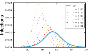
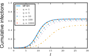
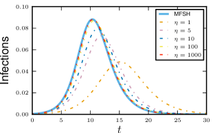
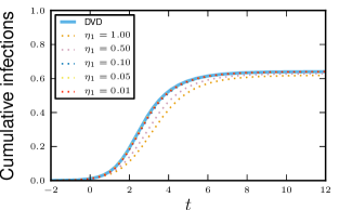
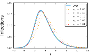
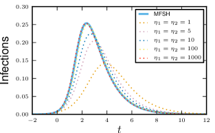
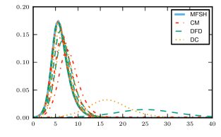
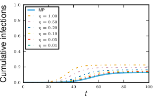
We show convergence of the DVD model to the MP and MFSH heterogeneity model as η0𝜂0\eta\to 0 or η𝜂\eta\to\infty in figure 3. The technical mathematical details showing this convergence are in the Appendix.
Refer to caption
Refer to caption
Refer to caption
Refer to caption
Figure 3: Convergence of DVD to MP and MFSH models. We consider the DVD model with varying values of η𝜂\eta. The probability density function for the expected degree is ρ(κ)=eκ/[exp(10)1]𝜌𝜅superscript𝑒𝜅delimited-[]101\rho(\kappa)=e^{\kappa}/[\exp(10)-1] for κ(0,10)𝜅010\kappa\in(0,10) and 00 otherwise. This yields Ψ(x)=[1exp(10(1x))]/[10(1x)]Ψ𝑥delimited-[]1101𝑥delimited-[]101𝑥\Psi(x)=[1-\exp(-10(1-x))]/[10(1-x)]. We take β=0.2𝛽0.2\beta=0.2 and γ=1𝛾1\gamma=1. As η𝜂\eta decreases (top), the MP model results, while as η𝜂\eta increases (bottom) the MFSH model results. Note the difference in axes from top to bottom.

3.2 Actual degree models

For our second class of models, we assume that each node has an actual degree k𝑘k assigned using the probability mass function P(k)𝑃𝑘P(k). The degree must be a non-negative integer. Each individual is given k𝑘k stubs, and at any time those stubs may join in pairs with stubs of other nodes to form edges. In most models we assume that the stubs are always in pairs (though the partner may change), so the degree is k𝑘k. In the Dormant Contact model, we allow stubs to be active or dormant, and thus take kmsubscript𝑘𝑚k_{m} [distributed according to P(km)𝑃subscript𝑘𝑚P(k_{m})] to be the maximum degree of a node, with kasubscript𝑘𝑎k_{a} and kdsubscript𝑘𝑑k_{d} the active and dormant degrees respectively ka+kd=kmsubscript𝑘𝑎subscript𝑘𝑑subscript𝑘𝑚k_{a}+k_{d}=k_{m}. We use θ(t)𝜃𝑡\theta(t) to denote the probability that a stub has not transmitted infection from a neighbor to its node by time t𝑡t. The probability a node with a given k𝑘k is susceptible is θksuperscript𝜃𝑘\theta^{k}, and taking a weighted average over all k𝑘k, we find S(t)=ψ(θ(t))𝑆𝑡𝜓𝜃𝑡S(t)=\psi(\theta(t)) where

ψ(x)=kP(k)xk𝜓𝑥subscript𝑘𝑃𝑘superscript𝑥𝑘\psi(x)=\sum_{k}P(k)x^{k}

3.2.1 Configuration Model

The Configuration Model (CM) networks are similar to the MP networks. In a CM network, the exact degree of an individual is assigned. A node is given k𝑘k stubs, assigned using the probability mass function P(k)𝑃𝑘P(k). Once all stubs are assigned to nodes, stubs are randomly paired into edges. The resulting network is static. We define θ𝜃\theta to be the probability that the neighbor along a random stub from u𝑢u has not transmitted infection to u𝑢u (so 1θ1𝜃1-\theta is the probability the neighbor has transmitted). We find that

θ˙˙𝜃\displaystyle\dot{\theta} =βθ+βψ(θ)ψ(1)+γ(1θ)absent𝛽𝜃𝛽superscript𝜓𝜃superscript𝜓1𝛾1𝜃\displaystyle=-\beta\theta+\beta\frac{\psi^{\prime}(\theta)}{\psi^{\prime}(1)}+\gamma(1-\theta)
R˙˙𝑅\displaystyle\dot{R} =γI,S=ψ(θ),I=1SRformulae-sequenceabsent𝛾𝐼formulae-sequence𝑆𝜓𝜃𝐼1𝑆𝑅\displaystyle=\gamma I\,,\qquad\qquad S=\psi(\theta)\,,\qquad\qquad I=1-S-R

This is similar to the MP model. In fact, it is possible to show that a MP network is a special case of the CM networks. In MP networks, a node u𝑢u with expected degree κusubscript𝜅𝑢\kappa_{u} has its actual degree chosen from a Poisson distribution of mean κusubscript𝜅𝑢\kappa_{u} (in the limit of a large network). Thus in an MP network the probability a node has degree k𝑘k is P(k)=0[eκκk/k!]ρ(κ)dκ𝑃𝑘superscriptsubscript0delimited-[]superscript𝑒𝜅superscript𝜅𝑘𝑘𝜌𝜅differential-d𝜅P(k)=\int_{0}^{\infty}[e^{-\kappa}\kappa^{k}/k!]\rho(\kappa)\,\mathrm{d}\kappa. Thus ψ(x)=kP(k)xk=0eκ(κkxk/k!)ρ(κ)dκ=Ψ(x)𝜓𝑥subscript𝑘𝑃𝑘superscript𝑥𝑘superscriptsubscript0superscript𝑒𝜅superscript𝜅𝑘superscript𝑥𝑘𝑘𝜌𝜅differential-d𝜅Ψ𝑥\psi(x)=\sum_{k}P(k)x^{k}=\int_{0}^{\infty}e^{-\kappa}(\sum\kappa^{k}x^{k}/k!)\rho(\kappa)\,\mathrm{d}\kappa=\Psi(x), and so the MP model emerges as a special case of the CM model.

3.2.2 Mean Field Social Heterogeneity [actual degree formulation]

In the actual degree version of Mean Field Social Heterogeneity (MFSH), each individual has k𝑘k stubs. Stubs change neighbors quickly so that the neighbor at any given time has no bearing on who the neighbor is later. The governing equations are

θ˙˙𝜃\displaystyle\dot{\theta} =βθ+βθθψ(θ)ψ(1)γθlnθabsent𝛽𝜃𝛽𝜃𝜃superscript𝜓𝜃superscript𝜓1𝛾𝜃𝜃\displaystyle=-\beta\theta+\beta\theta\frac{\theta\psi^{\prime}(\theta)}{\psi^{\prime}(1)}-\gamma\theta\ln\theta
R˙˙𝑅\displaystyle\dot{R} =γI,S=ψ(θ),I=1SRformulae-sequenceabsent𝛾𝐼formulae-sequence𝑆𝜓𝜃𝐼1𝑆𝑅\displaystyle=\gamma I\,,\qquad\qquad S=\psi(\theta)\,,\qquad\qquad I=1-S-R

Using techniques similar to those for the expected degree formulation of the MFSH model, we can show that if all degrees are the same, then this reduces to the MA model. Similarly, if the degrees are sufficiently close to the mean degree in the sense that K4/K41delimited-⟨⟩superscript𝐾4superscriptdelimited-⟨⟩𝐾41\left\langle K^{4}\right\rangle/\left\langle K\right\rangle^{4}\to 1 and both γ𝛾\gamma and βK𝛽delimited-⟨⟩𝐾\beta\left\langle K\right\rangle are fixed, then the solution again converges to that of the MA model. In section 3.3.1 we show that in fact this model is equivalent to the expected degree formulation of the MFSH model.

3.2.3 Dynamic Fixed-Degree

In the Dynamic Fixed-Degree (DFD) model a node is given k𝑘k stubs, which are paired with stubs of other nodes into edges. As time progresses, an edge may break, and the freed stubs immediately form edges with stubs from other edges that break at the same time, a process we refer to as “edge swapping”. The rate any edge breaks is η𝜂\eta. The resulting equations are

θ˙˙𝜃\displaystyle\dot{\theta} =βϕI,absent𝛽subscriptitalic-ϕ𝐼\displaystyle=-\beta\phi_{I}\,,
ϕ˙Ssubscript˙italic-ϕ𝑆\displaystyle\dot{\phi}_{S} =βϕIϕSψ′′(θ)ψ(θ)+ηθπSηϕS,absent𝛽subscriptitalic-ϕ𝐼subscriptitalic-ϕ𝑆superscript𝜓′′𝜃superscript𝜓𝜃𝜂𝜃subscript𝜋𝑆𝜂subscriptitalic-ϕ𝑆\displaystyle=-\beta\phi_{I}\phi_{S}\frac{\psi^{\prime\prime}(\theta)}{\psi^{\prime}(\theta)}+\eta\theta\pi_{S}-\eta\phi_{S}\,,
ϕ˙Isubscript˙italic-ϕ𝐼\displaystyle\dot{\phi}_{I} =βϕIϕSψ′′(θ)ψ(θ)+ηθπI(β+γ+η)ϕI,absent𝛽subscriptitalic-ϕ𝐼subscriptitalic-ϕ𝑆superscript𝜓′′𝜃superscript𝜓𝜃𝜂𝜃subscript𝜋𝐼𝛽𝛾𝜂subscriptitalic-ϕ𝐼\displaystyle=\beta\phi_{I}\phi_{S}\frac{\psi^{\prime\prime}(\theta)}{\psi^{\prime}(\theta)}+\eta\theta\pi_{I}-(\beta+\gamma+\eta)\phi_{I}\,,
π˙Rsubscript˙𝜋𝑅\displaystyle\dot{\pi}_{R} =γπI,πS=θψ(θ)ψ(1),πI=1πRπS,formulae-sequenceabsent𝛾subscript𝜋𝐼formulae-sequencesubscript𝜋𝑆𝜃superscript𝜓𝜃superscript𝜓1subscript𝜋𝐼1subscript𝜋𝑅subscript𝜋𝑆\displaystyle=\gamma\pi_{I}\,,\qquad\qquad\pi_{S}=\frac{\theta\psi^{\prime}(\theta)}{\psi^{\prime}(1)}\,,\qquad\qquad\pi_{I}=1-\pi_{R}-\pi_{S}\,,
R˙˙𝑅\displaystyle\dot{R} =γI,S(t)=ψ(θ),I(t)=1SR.formulae-sequenceabsent𝛾𝐼formulae-sequence𝑆𝑡𝜓𝜃𝐼𝑡1𝑆𝑅\displaystyle=\gamma I\,,\qquad\qquad S(t)=\psi(\theta)\,,\qquad\qquad I(t)=1-S-R\,.

The new variables ϕSsubscriptitalic-ϕ𝑆\phi_{S} and ϕIsubscriptitalic-ϕ𝐼\phi_{I} represent the probability that a stub has not transmitted infection from any neighbor to its node and is currently connected to a susceptible or infected neighbor respectively. The variables were not needed in the earlier models because we can solve for them explicitly in those cases. The new variables πSsubscript𝜋𝑆\pi_{S}, πIsubscript𝜋𝐼\pi_{I}, and πRsubscript𝜋𝑅\pi_{R} represent the proportion of all stubs that belong to susceptible, infected, or recovered nodes. A newly formed edge connects a node to a susceptible, infected, or recovered node with probabilities πSsubscript𝜋𝑆\pi_{S}, πIsubscript𝜋𝐼\pi_{I}, and πRsubscript𝜋𝑅\pi_{R} respectively.

The DFD model plays the same role in the actual degree case that DVD model played in the expcted degree case. It experiences similar limiting behavior. If η/β𝜂𝛽\eta/\beta is large, we recover the MFSH model. Alternately the CM is an accurate approximation so long as η(tt0)𝜂𝑡subscript𝑡0\eta(t-t_{0}) is small where t0subscript𝑡0t_{0} is a time around when the epidemic begins to infect significant numbers. Again, a more precise condition that η(πI+πR)/r1much-less-than𝜂subscript𝜋𝐼subscript𝜋𝑅𝑟1\eta(\pi_{I}+\pi_{R})/r\ll 1 where r𝑟r is the early exponential growth rate is described in the Appendix.

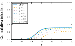
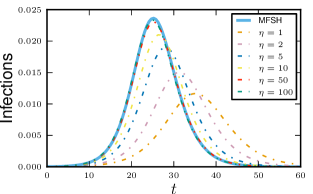
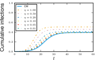
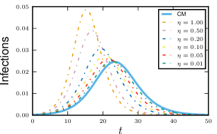
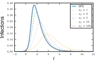
Figure 4 shows the convergence of this model to the CM and MFSH models as η0𝜂0\eta\to 0 or η𝜂\eta\to\infty.

Refer to caption
Refer to caption
Refer to caption
Refer to caption
Figure 4: Convergence of DFD to CM and MFSH models. We consider the DFD model with varying values of η𝜂\eta. The degrees are k=6𝑘6k=6,  k=8𝑘8k=8, and k=10𝑘10k=10, with probability 1/3131/3 each. This yields ψ(x)=(x6+x8+x10)/3𝜓𝑥superscript𝑥6superscript𝑥8superscript𝑥103\psi(x)=(x^{6}+x^{8}+x^{10})/3. We take β=0.2𝛽0.2\beta=0.2 and γ=1𝛾1\gamma=1. As η𝜂\eta decreases (top), the CM model results, while as η𝜂\eta increases (bottom) the MFSH model results. Note the difference in axes from top to bottom.

3.2.4 Dormant Contacts

Refer to caption
Refer to caption
Refer to caption
Refer to caption
Refer to caption
Refer to caption
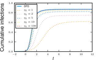
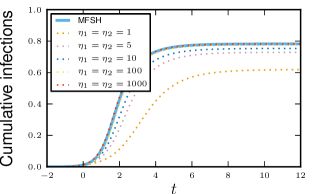
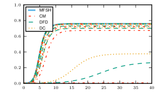
Figure 5: Convergence of DC to DFD, DVD, and MFSH models. We take β=γ=1𝛽𝛾1\beta=\gamma=1. (top) We consider the convergence of the DC model to the DFD model as η1subscript𝜂1\eta_{1} increases. We take ψ(x)=(x2+x8)/2𝜓𝑥superscript𝑥2superscript𝑥82\psi(x)=(x^{2}+x^{8})/2. For the DC model we take η2=1subscript𝜂21\eta_{2}=1 and vary η1subscript𝜂1\eta_{1}. As η1subscript𝜂1\eta_{1} increases, the DC model converges to the DFD model result for η=1𝜂1\eta=1. (middle) We consider the convergence of the DC model to the DVD model as η1subscript𝜂1\eta_{1} decreases and the degrees increase to compensate. For the DC model, we have ψ(x)=(x1/ξ+x4/ξ)/2𝜓𝑥superscript𝑥1𝜉superscript𝑥4𝜉2\psi(x)=(x^{1/\xi}+x^{4/\xi})/2 where ξ=η1/(η1+η2)𝜉subscript𝜂1subscript𝜂1subscript𝜂2\xi=\eta_{1}/(\eta_{1}+\eta_{2}). We use η2=1subscript𝜂21\eta_{2}=1 and vary η1subscript𝜂1\eta_{1}. For the DVD model, we take η=1𝜂1\eta=1 and Ψ(x)=(exp[(1x)]+exp[4(1x)])/2Ψ𝑥1𝑥41𝑥2\Psi(x)=(\exp[-(1-x)]+\exp[-4(1-x)])/2. (bottom) We consider the convergence of the DC model to the MFSH model with η1=η2subscript𝜂1subscript𝜂2\eta_{1}=\eta_{2} and η1,η2subscript𝜂1subscript𝜂2\eta_{1},\eta_{2}\to\infty. We take ψ(x)=(x2+x8)/2𝜓𝑥superscript𝑥2superscript𝑥82\psi(x)=(x^{2}+x^{8})/2. The MFSH model has the same ψ𝜓\psi, but uses βξ=β/2𝛽𝜉𝛽2\beta\xi=\beta/2 as the transmission rate. Note that for all three calculations, the η1=1subscript𝜂11\eta_{1}=1 curves are the same.

We finally move to the Dormant Contact (DC) model which captures all the previous expected and actual degree models as limiting cases. In the DC model, each node is given kmsubscript𝑘𝑚k_{m} stubs [with kmsubscript𝑘𝑚k_{m} chosen from P(km)𝑃subscript𝑘𝑚P(k_{m})]. However, only a fraction of them are active. At any given time, the node will have kasubscript𝑘𝑎k_{a} active stubs and kdsubscript𝑘𝑑k_{d} dormant stubs, so km=ka+kdsubscript𝑘𝑚subscript𝑘𝑎subscript𝑘𝑑k_{m}=k_{a}+k_{d} is the maximum number of active stubs. Active stubs become dormant at rate η2subscript𝜂2\eta_{2} and dormant stubs become active at rate η1subscript𝜂1\eta_{1}. We take ψ(x)=kmP(km)xkm𝜓𝑥subscriptsubscript𝑘𝑚𝑃subscript𝑘𝑚superscript𝑥subscript𝑘𝑚\psi(x)=\sum_{k_{m}}P(k_{m})x^{k_{m}}. The governing equations are

θ˙˙𝜃\displaystyle\dot{\theta} =βϕIabsent𝛽subscriptitalic-ϕ𝐼\displaystyle=-\beta\phi_{I}
ϕ˙Ssubscript˙italic-ϕ𝑆\displaystyle\dot{\phi}_{S} =βϕIϕSψ′′(θ)ψ(θ)+η1πSπϕDη2ϕSabsent𝛽subscriptitalic-ϕ𝐼subscriptitalic-ϕ𝑆superscript𝜓′′𝜃superscript𝜓𝜃subscript𝜂1subscript𝜋𝑆𝜋subscriptitalic-ϕ𝐷subscript𝜂2subscriptitalic-ϕ𝑆\displaystyle=-\beta\phi_{I}\phi_{S}\frac{\psi^{\prime\prime}(\theta)}{\psi^{\prime}(\theta)}+\eta_{1}\frac{\pi_{S}}{\pi}\phi_{D}-\eta_{2}\phi_{S}
ϕ˙Isubscript˙italic-ϕ𝐼\displaystyle\dot{\phi}_{I} =βϕIϕSψ′′(θ)ψ(θ)+η1πIπϕD(η2+β+γ)ϕIabsent𝛽subscriptitalic-ϕ𝐼subscriptitalic-ϕ𝑆superscript𝜓′′𝜃superscript𝜓𝜃subscript𝜂1subscript𝜋𝐼𝜋subscriptitalic-ϕ𝐷subscript𝜂2𝛽𝛾subscriptitalic-ϕ𝐼\displaystyle=\beta\phi_{I}\phi_{S}\frac{\psi^{\prime\prime}(\theta)}{\psi^{\prime}(\theta)}+\eta_{1}\frac{\pi_{I}}{\pi}\phi_{D}-(\eta_{2}+\beta+\gamma)\phi_{I}
ϕ˙Dsubscript˙italic-ϕ𝐷\displaystyle\dot{\phi}_{D} =η2(θϕD)η1ϕDabsentsubscript𝜂2𝜃subscriptitalic-ϕ𝐷subscript𝜂1subscriptitalic-ϕ𝐷\displaystyle=\eta_{2}(\theta-\phi_{D})-\eta_{1}\phi_{D}
ξ˙Rsubscript˙𝜉𝑅\displaystyle\dot{\xi}_{R} =η2ξR+η1πR+γξI,ξS=(θϕD)ψ(θ)ψ(1),ξI=ξξSξRformulae-sequenceabsentsubscript𝜂2subscript𝜉𝑅subscript𝜂1subscript𝜋𝑅𝛾subscript𝜉𝐼formulae-sequencesubscript𝜉𝑆𝜃subscriptitalic-ϕ𝐷superscript𝜓𝜃superscript𝜓1subscript𝜉𝐼𝜉subscript𝜉𝑆subscript𝜉𝑅\displaystyle=-\eta_{2}\xi_{R}+\eta_{1}\pi_{R}+\gamma\xi_{I}\,,\qquad\xi_{S}=(\theta-\phi_{D})\frac{\psi^{\prime}(\theta)}{\psi^{\prime}(1)}\,,\qquad\xi_{I}=\xi-\xi_{S}-\xi_{R}
π˙Rsubscript˙𝜋𝑅\displaystyle\dot{\pi}_{R} =η2ξRη1πR+γπI,πS=ϕDψ(θ)ψ(1),πI=ππSπRformulae-sequenceabsentsubscript𝜂2subscript𝜉𝑅subscript𝜂1subscript𝜋𝑅𝛾subscript𝜋𝐼formulae-sequencesubscript𝜋𝑆subscriptitalic-ϕ𝐷superscript𝜓𝜃superscript𝜓1subscript𝜋𝐼𝜋subscript𝜋𝑆subscript𝜋𝑅\displaystyle=\eta_{2}\xi_{R}-\eta_{1}\pi_{R}+\gamma\pi_{I}\,,\qquad\pi_{S}=\phi_{D}\frac{\psi^{\prime}(\theta)}{\psi^{\prime}(1)}\,,\qquad\pi_{I}=\pi-\pi_{S}-\pi_{R}
ξ𝜉\displaystyle\xi =η1η1+η2,π=η2η1+η2formulae-sequenceabsentsubscript𝜂1subscript𝜂1subscript𝜂2𝜋subscript𝜂2subscript𝜂1subscript𝜂2\displaystyle=\frac{\eta_{1}}{\eta_{1}+\eta_{2}}\,,\qquad\pi=\frac{\eta_{2}}{\eta_{1}+\eta_{2}}
R˙˙𝑅\displaystyle\dot{R} =γI,S=ψ(θ),I=1SRformulae-sequenceabsent𝛾𝐼formulae-sequence𝑆𝜓𝜃𝐼1𝑆𝑅\displaystyle=\gamma I\,,\qquad\qquad S=\psi(\theta)\,,\qquad\qquad I=1-S-R

The new variable ϕDsubscriptitalic-ϕ𝐷\phi_{D} represents the probability that a stub has not transmitted infection to its node and is currently dormant. The variables πSsubscript𝜋𝑆\pi_{S}, πIsubscript𝜋𝐼\pi_{I}, and πRsubscript𝜋𝑅\pi_{R} now measure the proportion of all stubs which are both dormant and belong to a susceptible, infected, or recovered node, with π=πS+πI+πR=η2/(η1+η2)𝜋subscript𝜋𝑆subscript𝜋𝐼subscript𝜋𝑅subscript𝜂2subscript𝜂1subscript𝜂2\pi=\pi_{S}+\pi_{I}+\pi_{R}=\eta_{2}/(\eta_{1}+\eta_{2}) the probability a stub is dormant. The ratios πS/πsubscript𝜋𝑆𝜋\pi_{S}/\pi, πI/πsubscript𝜋𝐼𝜋\pi_{I}/\pi, and πR/πsubscript𝜋𝑅𝜋\pi_{R}/\pi give the probabilities that a newly formed edge connects to a susceptbile, infected, or recovered node. The variables ξSsubscript𝜉𝑆\xi_{S}, ξIsubscript𝜉𝐼\xi_{I}, and ξRsubscript𝜉𝑅\xi_{R} give the probabilities that a stub is active and belongs to a susceptible, infected, or recovered node, with ξ=ξS+ξI+ξR=η1/(η1+η2)𝜉subscript𝜉𝑆subscript𝜉𝐼subscript𝜉𝑅subscript𝜂1subscript𝜂1subscript𝜂2\xi=\xi_{S}+\xi_{I}+\xi_{R}=\eta_{1}/(\eta_{1}+\eta_{2}) the probability a stub is active.

It is relatively straightforward to see that if η1subscript𝜂1\eta_{1} is much larger than η2subscript𝜂2\eta_{2}, then the proportion of time a stub is dormant is tiny, π1much-less-than𝜋1\pi\ll 1. Consequently at any moment a node is expected to have ka=(1π)kmkmsubscript𝑘𝑎1𝜋subscript𝑘𝑚subscript𝑘𝑚k_{a}=(1-\pi)k_{m}\approx k_{m} active contacts. As η2/η1subscript𝜂2subscript𝜂1\eta_{2}/\eta_{1} shrinks, this approximation improves. So in this limit, the DC model should reduce to the DFD model with edges breaking at rate η2subscript𝜂2\eta_{2}. Indeed, in the equations above, if we take η=η2𝜂subscript𝜂2\eta=\eta_{2} and assume η1ηmuch-greater-thansubscript𝜂1𝜂\eta_{1}\gg\eta, then ϕDsubscriptitalic-ϕ𝐷\phi_{D} is negligibly small, so the ϕDsubscriptitalic-ϕ𝐷\phi_{D} terms drop out of the ϕSsubscriptitalic-ϕ𝑆\phi_{S} and ϕIsubscriptitalic-ϕ𝐼\phi_{I} equations. The values of πSsubscript𝜋𝑆\pi_{S} and πIsubscript𝜋𝐼\pi_{I} both go to zero as η1subscript𝜂1\eta_{1} grows, but a little more care shows that πS/πsubscript𝜋𝑆𝜋\pi_{S}/\pi approaches ξSsubscript𝜉𝑆\xi_{S} and πI/πsubscript𝜋𝐼𝜋\pi_{I}/\pi approaches ξIsubscript𝜉𝐼\xi_{I} and the ξ𝜉\xi variables solve the same equations in this limit as the π𝜋\pi variables in the DFD equations. Thus the DC equations reduce to the DFD equations in this limit. More details are in the Appendix.

In the opposite limit, if η2subscript𝜂2\eta_{2} is large compared to η1subscript𝜂1\eta_{1}, then stubs spend most time dormant, ξ1much-less-than𝜉1\xi\ll 1. If the number of stubs is sufficiently large, the expected number of active stubs κ=𝔼[ka]=ξkm𝜅𝔼delimited-[]subscript𝑘𝑎𝜉subscript𝑘𝑚\kappa=\mathbb{E}[k_{a}]=\xi k_{m} will not be negligible. The variation in the number of active stubs will be significant relative to its expected value κ𝜅\kappa. However, κkmmuch-less-than𝜅subscript𝑘𝑚\kappa\ll k_{m} so the number of dormant stubs kd=kmkasubscript𝑘𝑑subscript𝑘𝑚subscript𝑘𝑎k_{d}=k_{m}-k_{a} can be approximated as kmπsubscript𝑘𝑚𝜋k_{m}\pi. The rate that dormant stubs become active is η1subscript𝜂1\eta_{1}, so the rate at which the node forms new edges is approximately η1kd=η1kmπsubscript𝜂1subscript𝑘𝑑subscript𝜂1subscript𝑘𝑚𝜋\eta_{1}k_{d}=\eta_{1}k_{m}\pi which itself is η2κsubscript𝜂2𝜅\eta_{2}\kappa, while each existing edge breaks at rate η2subscript𝜂2\eta_{2}. This is the assumption underlying the DVD model. A careful analysis of the equations show that indeed we can reduce them to the DVD model if η2η1much-greater-thansubscript𝜂2subscript𝜂1\eta_{2}\gg\eta_{1}. More details are in the Appendix.

Alternately, we can have the DC model converge to the MFSH model if Kdelimited-⟨⟩𝐾\left\langle K\right\rangle\to\infty, as long as βK𝛽delimited-⟨⟩𝐾\beta\left\langle K\right\rangle remains fixed. In this case we find that the MFSH model is a good approximation, using β^=βξ^𝛽𝛽𝜉\hat{\beta}=\beta\xi as the transmission rate. The underlying argument of this is that as Kdelimited-⟨⟩𝐾\left\langle K\right\rangle increases, the probability of transmission per edge decreases. Consequently, it becomes unimportant whether the edge has long or short duration because it is incredibly rare for the disease to try to transmit along the same edge twice. The total infectiousness of an individual is then given by the number of active edges times the per-edge infection rate. We can assume that only a proportion ξ𝜉\xi of the stubs are active at any time, and we can absorb this into β𝛽\beta. So an individual with k𝑘k stubs causes transmission at rate β^k^𝛽𝑘\hat{\beta}k where β^=ξβ^𝛽𝜉𝛽\hat{\beta}=\xi\beta. This is independent of how (or if) the edges are changing in time.

Figure 5 shows how the DC model reduces in the various limits.

3.3 Further Analysis of Mean Field Social Heterogeneity models

In this section we show that the two MFSH models are equivalent. We also show that all the non-Mass Action models described here reduce to the MFSH model if the average number of contacts is large, and the probability of infection per edge scales like 1/K1delimited-⟨⟩𝐾1/\left\langle K\right\rangle. Technically, our results show that there is no difference between the results of any of the (non-MA) models in this limit, so any of these models would be appropriate, but generally the equations of the MFSH model are simplest so we use it.

3.3.1 Equivalence of Mean Field Social Heterogeneity formulations

There are two formulations of the MFSH model, one with expected degrees and the other with actual degrees.

In the expected degree formulation, each individual has an expected degree κ𝜅\kappa. On average, at any given moment of time the individual has κ𝜅\kappa contacts. The exact number of contacts may vary from moment to moment, but how many contacts exist at one moment and who those contacts are with are independent from any other moment. Thus over a short period of time, we may safely assume that the total number of contacts with infected individuals matches the expected number.

In the actual degree formulation, each individual is assigned an actual degree k𝑘k and given k𝑘k stubs. At any time each of those k𝑘k stubs forms an edge with a stub from another node, but who the stub connects to changes rapidly. Again, over a short period of time, we may assume that the number of contacts with infected individuals matches the expected number.

Actual degree formulation as a special case of expected degree formulation

Because contacts are very short, over any time interval, the total contact time is well-approximated based on the expected amount of contact at any given moment. Thus whether the individuals have the same number of contacts at each moment, or whether the amount varies from moment to moment, the effect over any macroscopic time interval is the same. Thus the actual degree model should be a special case of the expected degree model. In the expected degree formulation, the probability that a node with κ𝜅\kappa expected contacts is susceptible is exp[κ(1Θ)]𝜅1Θ\exp[-\kappa(1-\Theta)] and in the actual degree formulation the probability that a node with k𝑘k contacts is susceptible is θksuperscript𝜃𝑘\theta^{k}. If κ=k𝜅𝑘\kappa=k, we expect these to equal, and so we anticipate θ=exp(Θ1)𝜃Θ1\theta=\exp(\Theta-1), or Θ=1+lnθΘ1𝜃\Theta=1+\ln\theta. Plugging this into the expected degree equations, we arrive at the actual degree equations. So the two methods are equivalent subject to a change in variables.

Expected degree formulation as a limiting case of the actual degree formulation

The fact that the actual degree formulation leads to the expected degree formulation is based on similar reasoning. The underlying additional idea is that any continuous distribution can be approximated by a sufficiently well-refined discrete distribution. We then need a way to take a well-refined discrete distribution and rescale it so that all the probability is massed at integer values. To do this we make the observation that we can multiply everyone’s (expected or actual) degree by L𝐿L with no impact on the epidemic so long as we also divide the transmission rate by L𝐿L.

To make this more precise, consider a given β𝛽\beta and ρ(κ)𝜌𝜅\rho(\kappa) and assume L𝐿L is large. We approximate the continuous distribution of κ𝜅\kappa using a discrete distribution where the probability of k/L𝑘𝐿k/L is k/L(k+1)/Lρ(κ)dκsuperscriptsubscript𝑘𝐿𝑘1𝐿𝜌𝜅differential-d𝜅\int_{k/L}^{(k+1)/L}\rho(\kappa)\,\mathrm{d}\kappa. Increasing L𝐿L gives a finer scale approximation. We then multiply every k/L𝑘𝐿k/L by L𝐿L, to get P(k)=k/L(k+1)/Lρ(κ)dκ𝑃𝑘superscriptsubscript𝑘𝐿𝑘1𝐿𝜌𝜅differential-d𝜅P(k)=\int_{k/L}^{(k+1)/L}\rho(\kappa)\,\mathrm{d}\kappa where k𝑘k is an integer. So long as we divide β𝛽\beta by L𝐿L, the spread of the epidemic on a population with the given P(k)𝑃𝑘P(k) and the rescaled β𝛽\beta will closely approximate the epidemic spread in the original expected degree population, with the approximation improving as L𝐿L\to\infty. We find that the actual degree equations converge to the expected degree equations as L𝐿L\to\infty. Full details are in the Appendix.

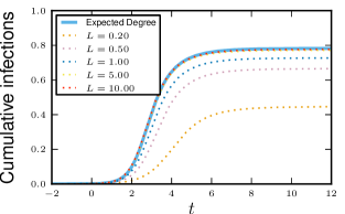
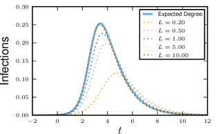
As an example we take the uniform distribution from 00 to 101010 for κ𝜅\kappa. So Ψ(x)=(1exp[10(1Θ)])/[2(1Θ)]Ψ𝑥1101Θdelimited-[]21Θ\Psi(x)=(1-\exp[-10(1-\Theta)])/[2(1-\Theta)]. We initially start with a discrete distribution on the integers 00 through 999 with weight 1/101101/10 on each. So our initial ψ(x)𝜓𝑥\psi(x) is k=09xk/10=(x101)/10(x1)superscriptsubscript𝑘09superscript𝑥𝑘10superscript𝑥10110𝑥1\sum_{k=0}^{9}x^{k}/10=(x^{10}-1)/10(x-1) with β=β^𝛽^𝛽\beta=\hat{\beta}. We then refine the distribution. For given L𝐿L we have ψ(x)=k=010L1xk/10L=(x10L1)/[10L(x1)]𝜓𝑥superscriptsubscript𝑘010𝐿1superscript𝑥𝑘10𝐿superscript𝑥10𝐿1delimited-[]10𝐿𝑥1\psi(x)=\sum_{k=0}^{10L-1}x^{k}/10L=(x^{10L}-1)/[10L(x-1)], and we take β=β^/L𝛽^𝛽𝐿\beta=\hat{\beta}/L. Convergence is shown in figure 6.

Refer to caption
Refer to caption
Figure 6: Convergence of actual degree formulation of MFSH to expected degree formulation. The actual degree formulation of the MFSH model for the appropriate discrete distribution (described in text) converges to the expected degree formulation of the MFSH model with contact rates chosen uniformly from 00 to 101010.

3.3.2 Reduction of all models to Mean Field Social Heterogeneity model at large average degree

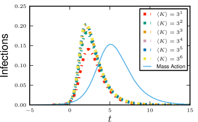
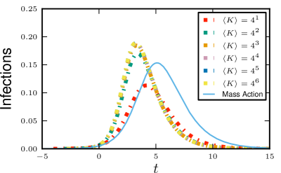
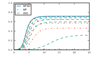
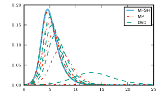
One particularly important limit corresponds to people having many contacts, but a low probability of transmitting per contact before recovering. That is, Kdelimited-⟨⟩𝐾\left\langle K\right\rangle is large, and β/γ𝛽𝛾\beta/\gamma is comparably small. In this limit, we expect that the duration of contact becomes unimportant, because the infection is unlikely to cross an edge more than once so it has no way to know how long the edge lasts. Heterogeneity in contact levels may still play an important role. If the heterogeneity is sufficiently small, it is reasonable to expect that the MA SIR model is appropriate.

In section 4.2 we rigorously derive the MFSH model from the DC model assuming Kdelimited-⟨⟩𝐾\left\langle K\right\rangle\to\infty with fixed βK𝛽delimited-⟨⟩𝐾\beta\left\langle K\right\rangle and fixed γ𝛾\gamma. A similar proof will apply for the other models, or we can simply argue that the DC model reduces to all of the others, and careful attention to detail shows that they inherit this limiting case.
Refer to caption
Refer to caption
Refer to caption
Refer to caption
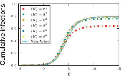
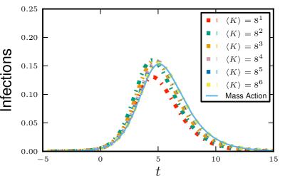
Figure 7: Convergence to MFSH. (top) Convergence of the Expected Degree models assuming a uniform distribution from 00 to 2K2delimited-⟨⟩𝐾2\left\langle K\right\rangle. (bottom) Convergence of the Actual Degree models assuming a third each with K/2delimited-⟨⟩𝐾2\left\langle K\right\rangle/2, Kdelimited-⟨⟩𝐾\left\langle K\right\rangle, and 3K/23delimited-⟨⟩𝐾23\left\langle K\right\rangle/2 stubs. The solid curves correspond to K=1delimited-⟨⟩𝐾1\left\langle K\right\rangle=1 (top) and K=2delimited-⟨⟩𝐾2\left\langle K\right\rangle=2 (bottom). The dotted curves correspond to various larger values of Kdelimited-⟨⟩𝐾\left\langle K\right\rangle. Because β𝛽\beta decreases to balance the increase in Kdelimited-⟨⟩𝐾\left\langle K\right\rangle, the MFSH curves are the same for all Kdelimited-⟨⟩𝐾\left\langle K\right\rangle.

3.3.3 Reduction of MFSH to MA model if K4/K41delimited-⟨⟩superscript𝐾4superscriptdelimited-⟨⟩𝐾41\left\langle K^{4}\right\rangle/\left\langle K\right\rangle^{4}\to 1 and βK𝛽delimited-⟨⟩𝐾\beta\left\langle K\right\rangle fixed

It is straightforward to show that the MFSH model becomes SIR model if every node has the same contact rate. However more generally, we would expect that if the contact rates are sufficiently close together, the model should behave like the SIR model. In fact this holds if K4/K41delimited-⟨⟩superscript𝐾4superscriptdelimited-⟨⟩𝐾41\left\langle K^{4}\right\rangle/\left\langle K\right\rangle^{4}\to 1 with βK𝛽delimited-⟨⟩𝐾\beta\left\langle K\right\rangle fixed. Intuitively, if the number of nodes with higher or lower contact rates is very small, their contribution to the spread of the disease is not significantly different from the contribution of an average node, and so the disease should spread as if the contact rate were homogeneous. We do not have a good intuitive explanation for why the precise condition relies on K4/K4delimited-⟨⟩superscript𝐾4superscriptdelimited-⟨⟩𝐾4\left\langle K^{4}\right\rangle/\left\langle K\right\rangle^{4}. However, we prove it rigorously in section 4.3.

We expect this case to be particularly relevant if the average degree is large and infectiousness is low. Combining this with the previous result, we conclude that all models converge to the MA model under appropriate conditions as Kdelimited-⟨⟩𝐾\left\langle K\right\rangle\to\infty.

4 Rigorous proof of convergence to Mass Action equations

In this section, we give a rigorous proof of one of the most significant results. Namely, if Kdelimited-⟨⟩𝐾\left\langle K\right\rangle is large, but K4/K4delimited-⟨⟩superscript𝐾4delimited-⟨⟩superscript𝐾4\left\langle K^{4}\right\rangle/\left\langle K^{4}\right\rangle is approximately 111 and βK𝛽delimited-⟨⟩𝐾\beta\left\langle K\right\rangle and γ𝛾\gamma are small compared to Kdelimited-⟨⟩𝐾\left\langle K\right\rangle, then regardless of which model we use, the result is well-approximated by the MA equations.

We first show some examples, and then provide the details needed to prove the result for the DC model. The simpler models can be derived in the same method (though in some cases the proof will be simpler). For our proof, we assume we have a sequence of populations and diseases indexed by n𝑛n such that Kdelimited-⟨⟩𝐾\left\langle K\right\rangle\to\infty,  K4/K41delimited-⟨⟩superscript𝐾4superscriptdelimited-⟨⟩𝐾41\left\langle K^{4}\right\rangle/\left\langle K\right\rangle^{4}\to 1 with ξβK𝜉𝛽delimited-⟨⟩𝐾\xi\beta\left\langle K\right\rangle fixed. We show that this converges to the mass action equations using β^=ξβK^𝛽𝜉𝛽delimited-⟨⟩𝐾\hat{\beta}=\xi\beta\left\langle K\right\rangle.

We show this in two steps.First, we show that in the limit of large Kdelimited-⟨⟩𝐾\left\langle K\right\rangle and constant βξK𝛽𝜉delimited-⟨⟩𝐾\beta\xi\left\langle K\right\rangle, the DC equations converge to the MFSH equations. We then show that the MFSH equations converge to the MA equations if additionally K4/K41delimited-⟨⟩superscript𝐾4superscriptdelimited-⟨⟩𝐾41\left\langle K^{4}\right\rangle/\left\langle K\right\rangle^{4}\to 1.

4.1 Example

Refer to caption
Refer to caption
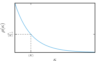
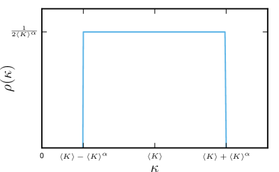
Figure 8: The expected degree distributions for our examples of convergence as Kdelimited-⟨⟩𝐾\left\langle K\right\rangle\to\infty, with and without K4/K41delimited-⟨⟩superscript𝐾4superscriptdelimited-⟨⟩𝐾41\left\langle K^{4}\right\rangle/\left\langle K\right\rangle^{4}\to 1.
Refer to caption
Refer to caption
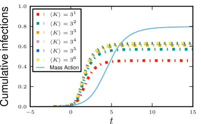
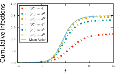
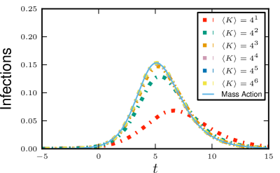
Figure 9: Sample convergence as Kdelimited-⟨⟩𝐾\left\langle K\right\rangle\to\infty. We use the exponential distribution described in figure 8. The distribution of expected degrees decays exponentially and K4/K4delimited-⟨⟩superscript𝐾4superscriptdelimited-⟨⟩𝐾4\left\langle K^{4}\right\rangle/\left\langle K\right\rangle^{4} does not approach 111 as Kdelimited-⟨⟩𝐾\left\langle K\right\rangle grows. The solutions appear to converge, but they do not converge to the MA SIR model.

As examples, we consider several different population structures using the MP model in figure 8. In the first, we take an exponential distribution of expected degrees. To vary the average degree, we change the decay rate of the exponential.

ρ(κ)=eκ/KK𝜌𝜅superscript𝑒𝜅delimited-⟨⟩𝐾delimited-⟨⟩𝐾\rho(\kappa)=\frac{e^{-\kappa/\left\langle K\right\rangle}}{\left\langle K\right\rangle}

This does not satisfy the conditions that K4/K41delimited-⟨⟩superscript𝐾4superscriptdelimited-⟨⟩𝐾41\left\langle K^{4}\right\rangle/\left\langle K\right\rangle^{4}\to 1. In the other examples, we take a uniform distribution, with expected degrees chosen uniformly from (KKα,K+Kα)delimited-⟨⟩𝐾superscriptdelimited-⟨⟩𝐾𝛼delimited-⟨⟩𝐾superscriptdelimited-⟨⟩𝐾𝛼(\left\langle K\right\rangle-\left\langle K\right\rangle^{\alpha},\left\langle K\right\rangle+\left\langle K\right\rangle^{\alpha}). That is,

ρ(κ)={0κ<KKα12KαKKα<κ<K+Kα0κ>K+K𝜌𝜅cases0𝜅delimited-⟨⟩𝐾superscriptdelimited-⟨⟩𝐾𝛼12superscriptdelimited-⟨⟩𝐾𝛼delimited-⟨⟩𝐾superscriptdelimited-⟨⟩𝐾𝛼𝜅delimited-⟨⟩𝐾superscriptdelimited-⟨⟩𝐾𝛼0𝜅delimited-⟨⟩𝐾delimited-⟨⟩𝐾\rho(\kappa)=\begin{cases}0&\kappa<\left\langle K\right\rangle-\left\langle K\right\rangle^{\alpha}\\ \frac{1}{2\left\langle K\right\rangle^{\alpha}}&\left\langle K\right\rangle-\left\langle K\right\rangle^{\alpha}<\kappa<\left\langle K\right\rangle+\left\langle K\right\rangle^{\alpha}\\ 0&\kappa>\left\langle K\right\rangle+\sqrt{\left\langle K\right\rangle}\end{cases}

This satisfies the condition for any α<1𝛼1\alpha<1. Using K^4delimited-⟨⟩superscript^𝐾4\left\langle\hat{K}^{4}\right\rangle to denote the average of the 444th power of the expected degree555Our condition that K4/K41delimited-⟨⟩superscript𝐾4superscriptdelimited-⟨⟩𝐾41\left\langle K^{4}\right\rangle/\left\langle K\right\rangle^{4}\to 1 applies equally for the fourth power of actual or expected degree since at leading order they are the same., we have K^4=K4+2K2+2α+K4α/5delimited-⟨⟩superscript^𝐾4superscriptdelimited-⟨⟩𝐾42superscriptdelimited-⟨⟩𝐾22𝛼superscriptdelimited-⟨⟩𝐾4𝛼5\left\langle\hat{K}^{4}\right\rangle=\left\langle K\right\rangle^{4}+2\left\langle K\right\rangle^{2+2\alpha}+\left\langle K\right\rangle^{4\alpha}/5. However, the condition fails for α=1𝛼1\alpha=1. The distribution would not make sense for α>1𝛼1\alpha>1 since some nodes would have negative expected degree.
Refer to caption
Refer to caption

α=1𝛼1\alpha=1

Refer to caption
Refer to caption

α=0.85𝛼0.85\alpha=0.85

Refer to caption
Refer to caption

α=0.5𝛼0.5\alpha=0.5

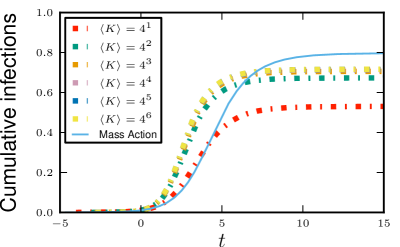
Figure 10: Sample convergence as Kdelimited-⟨⟩𝐾\left\langle K\right\rangle\to\infty. We use the uniform distribution described in figure 8. In the first, second, and third rows, we use α=1,0.85,0.5𝛼10.850.5\alpha=1,0.85,0.5 respectively. The condition fails for α=1𝛼1\alpha=1 and the solutions do not converge to the MA model, but they converge to the MA model for smaller α𝛼\alpha.

For all distributions, we take β=2/K𝛽2delimited-⟨⟩𝐾\beta=2/\left\langle K\right\rangle and γ=1𝛾1\gamma=1. The corresponding MA model has β^=2^𝛽2\hat{\beta}=2. In figure 9 we plot the results for the exponential distribution. This distribution does not satisfy the conditions, and we see that the solutions do converge, but not to the MA model. In figure 10, we take the uniform distribution from KKαdelimited-⟨⟩𝐾superscriptdelimited-⟨⟩𝐾𝛼\left\langle K\right\rangle-\left\langle K\right\rangle^{\alpha} to K+Kαdelimited-⟨⟩𝐾superscriptdelimited-⟨⟩𝐾𝛼\left\langle K\right\rangle+\left\langle K\right\rangle^{\alpha}. We again see that when the conditions are not satisfied, the solutions may still converge, but not to the corresponding MA model. However, when the conditions are satisfied, the solutions converge to the MA model.

4.2 DC to MFSH

We will use the following result several times in the proof: Assume g(t)𝑔𝑡g(t) is a function of time and

g˙=c(t)g+f(t)˙𝑔𝑐𝑡𝑔𝑓𝑡\dot{g}=-c(t)g+f(t)

If c(t)C>0𝑐𝑡𝐶0c(t)\geq C>0 for all time and |f|F𝑓𝐹|f|\leq F, and further |g(0)|F/C𝑔0𝐹𝐶|g(0)|\leq F/C, then for all time |g(t)|F/C𝑔𝑡𝐹𝐶|g(t)|\leq F/C. To see this, assume that f𝑓f and g𝑔g are positive. If g𝑔g is increasing beyond F/C𝐹𝐶F/C, then cg+f𝑐𝑔𝑓-cg+f must be negative, violating the assumption that g𝑔g is increasing. Similar results hold for negative values of f𝑓f and g𝑔g. Our proofs skip some of the intermediate steps. Complete details of all the algebra is in the Appendix.

We want to prove that if degrees increase, but simultaneously the infection rate decreases with γ𝛾\gamma constant then we must arrive at the Mass Action equations. We do this for the Dormant Contact model. We introduce the notation o(1)𝑜1o(1) to denote a function whose value goes to zero as Kdelimited-⟨⟩𝐾\left\langle K\right\rangle\to\infty. We will show that neglecting small terms in the large degree limit the DC model becomes

θ˙˙𝜃\displaystyle\dot{\theta} =β~θζabsent~𝛽𝜃𝜁\displaystyle=-\tilde{\beta}\theta\zeta
R˙˙𝑅\displaystyle\dot{R} =γI,S=ψ(θ),I=1SRformulae-sequenceabsent𝛾𝐼formulae-sequence𝑆𝜓𝜃𝐼1𝑆𝑅\displaystyle=\gamma I\,,\qquad S=\psi(\theta)\,,\qquad I=1-S-R

where ζ=1θψ(θ)/ψ(1)+(γ/β~)lnθ𝜁1𝜃superscript𝜓𝜃superscript𝜓1𝛾~𝛽𝜃\zeta=1-\theta\psi^{\prime}(\theta)/\psi^{\prime}(1)+(\gamma/\tilde{\beta})\ln\theta.

We define ζ=πI+ξI𝜁subscript𝜋𝐼subscript𝜉𝐼\zeta=\pi_{I}+\xi_{I} This is the proportion of all stubs which belong to infected nodes. We prove a series of results:

  1. 1.

    θ=1+o(1)𝜃1𝑜1\theta=1+o(1).

  2. 2.

    ϕD=π+o(1)subscriptitalic-ϕ𝐷𝜋𝑜1\phi_{D}=\pi+o(1).

  3. 3.

    ϕS=ξψ(θ)ψ(1)+o(1)subscriptitalic-ϕ𝑆𝜉superscript𝜓𝜃superscript𝜓1𝑜1\phi_{S}=\xi\frac{\psi^{\prime}(\theta)}{\psi^{\prime}(1)}+o(1).

  4. 4.

    πI=πζ+o(1)subscript𝜋𝐼𝜋𝜁𝑜1\pi_{I}=\pi\zeta+o(1)   ξI=ξζ+o(1)subscript𝜉𝐼𝜉𝜁𝑜1\xi_{I}=\xi\zeta+o(1).

  5. 5.

    ϕI=ξθζ+o(1)subscriptitalic-ϕ𝐼𝜉𝜃𝜁𝑜1\phi_{I}=\xi\theta\zeta+o(1)

  6. 6.

    θ˙=β~θζ+βo(1)˙𝜃~𝛽𝜃𝜁𝛽𝑜1\dot{\theta}=-\tilde{\beta}\theta\zeta+\beta o(1).

  7. 7.

    ζ=1θψ(θ)ψ(1)+(γ/β~)lnθ+to(1)𝜁1𝜃superscript𝜓𝜃superscript𝜓1𝛾~𝛽𝜃𝑡𝑜1\zeta=1-\theta\frac{\psi^{\prime}(\theta)}{\psi^{\prime}(1)}+(\gamma/\tilde{\beta})\ln\theta+to(1)

If we drop the error terms in the final two results, then we have the equations governing the Mean Field Social Heterogeneity model in the actual degree case, with β~=βξ~𝛽𝛽𝜉\tilde{\beta}=\beta\xi playing the role of the transmission rate. The existence of the error terms means that at earlier time, the approximation is better, and it can deviate more as time increases. The solution converges uniformly for any t𝑡t less than any arbitrary chosen value T𝑇T as Kdelimited-⟨⟩𝐾\left\langle K\right\rangle grows. So for large enough Kdelimited-⟨⟩𝐾\left\langle K\right\rangle, the region over which the MFSH model gives an accurate approximation will include the entire period of the epidemic.

  1. 1.

    θ=1+o(1)𝜃1𝑜1\theta=1+o(1).

    We trivially have 1θ1β/(β+γ)1𝜃1𝛽𝛽𝛾1\geq\theta\geq 1-\beta/(\beta+\gamma). Because βK𝛽delimited-⟨⟩𝐾\beta\left\langle K\right\rangle is constant, we find β=o(1)𝛽𝑜1\beta=o(1). Thus 1θ1+o(1)1𝜃1𝑜11\geq\theta\geq 1+o(1) (with a negative error term), and so we can conclude that θ=1+o(1)𝜃1𝑜1\theta=1+o(1).

  2. 2.

    ϕD=π+o(1)subscriptitalic-ϕ𝐷𝜋𝑜1\phi_{D}=\pi+o(1). We show ϕDπ=o(1)subscriptitalic-ϕ𝐷𝜋𝑜1\phi_{D}-\pi=o(1).

    ddt(ϕDπ)dd𝑡subscriptitalic-ϕ𝐷𝜋\displaystyle\frac{\mathrm{d}}{\mathrm{d}t}(\phi_{D}-\pi) =η2(θϕD)η1ϕDabsentsubscript𝜂2𝜃subscriptitalic-ϕ𝐷subscript𝜂1subscriptitalic-ϕ𝐷\displaystyle=\eta_{2}(\theta-\phi_{D})-\eta_{1}\phi_{D}
    =η2[1+o(1)](η1+η2)ϕDabsentsubscript𝜂2delimited-[]1𝑜1subscript𝜂1subscript𝜂2subscriptitalic-ϕ𝐷\displaystyle=\eta_{2}[1+o(1)]-(\eta_{1}+\eta_{2})\phi_{D}
    =(η1+η2)π(η1+η2)ϕD+o(1)absentsubscript𝜂1subscript𝜂2𝜋subscript𝜂1subscript𝜂2subscriptitalic-ϕ𝐷𝑜1\displaystyle=(\eta_{1}+\eta_{2})\pi-(\eta_{1}+\eta_{2})\phi_{D}+o(1)
    =(η1+η2)(ϕDπ)+o(1)absentsubscript𝜂1subscript𝜂2subscriptitalic-ϕ𝐷𝜋𝑜1\displaystyle=-(\eta_{1}+\eta_{2})(\phi_{D}-\pi)+o(1)

    In the next to last step we used the fact that π=η2/(η1+η2)𝜋subscript𝜂2subscript𝜂1subscript𝜂2\pi=\eta_{2}/(\eta_{1}+\eta_{2}) so η2=(η1+η2)πsubscript𝜂2subscript𝜂1subscript𝜂2𝜋\eta_{2}=(\eta_{1}+\eta_{2})\pi. So ϕDπsubscriptitalic-ϕ𝐷𝜋\phi_{D}-\pi is at most o(1)/(η1+η2)=o(1)𝑜1subscript𝜂1subscript𝜂2𝑜1o(1)/(\eta_{1}+\eta_{2})=o(1).

  3. 3.

    ϕS=ξψ(θ)ψ(1)+o(1)subscriptitalic-ϕ𝑆𝜉superscript𝜓𝜃superscript𝜓1𝑜1\phi_{S}=\xi\frac{\psi^{\prime}(\theta)}{\psi^{\prime}(1)}+o(1).

    We have

    ddt[ϕSξψ(θ)ψ(1)]dd𝑡delimited-[]subscriptitalic-ϕ𝑆𝜉superscript𝜓𝜃superscript𝜓1\displaystyle\frac{\mathrm{d}}{\mathrm{d}t}\left[\phi_{S}-\xi\frac{\psi^{\prime}(\theta)}{\psi^{\prime}(1)}\right] =ϕ˙Sξθ˙ψ′′(θ)ψ(1)absentsubscript˙italic-ϕ𝑆𝜉˙𝜃superscript𝜓′′𝜃superscript𝜓1\displaystyle=\dot{\phi}_{S}-\xi\dot{\theta}\frac{\psi^{\prime\prime}(\theta)}{\psi^{\prime}(1)}
    =η2ϕS+η1πSπϕDβϕIψ′′(θ)ψ(θ)(ϕSξψ(θ)ψ(1))absentsubscript𝜂2subscriptitalic-ϕ𝑆subscript𝜂1subscript𝜋𝑆𝜋subscriptitalic-ϕ𝐷𝛽subscriptitalic-ϕ𝐼superscript𝜓′′𝜃superscript𝜓𝜃subscriptitalic-ϕ𝑆𝜉superscript𝜓𝜃superscript𝜓1\displaystyle=-\eta_{2}\phi_{S}+\eta_{1}\frac{\pi_{S}}{\pi}\phi_{D}-\beta\phi_{I}\frac{\psi^{\prime\prime}(\theta)}{\psi^{\prime}(\theta)}\left(\phi_{S}-\xi\frac{\psi^{\prime}(\theta)}{\psi^{\prime}(1)}\right)
    =η2ϕS+η1πψ(θ)ψ(1)βϕIψ′′(θ)ψ(θ)(ϕSξψ(θ)ψ(1))+o(1)absentsubscript𝜂2subscriptitalic-ϕ𝑆subscript𝜂1𝜋superscript𝜓𝜃superscript𝜓1𝛽subscriptitalic-ϕ𝐼superscript𝜓′′𝜃superscript𝜓𝜃subscriptitalic-ϕ𝑆𝜉superscript𝜓𝜃superscript𝜓1𝑜1\displaystyle=-\eta_{2}\phi_{S}+\eta_{1}\pi\frac{\psi^{\prime}(\theta)}{\psi^{\prime}(1)}-\beta\phi_{I}\frac{\psi^{\prime\prime}(\theta)}{\psi^{\prime}(\theta)}\left(\phi_{S}-\xi\frac{\psi^{\prime}(\theta)}{\psi^{\prime}(1)}\right)+o(1)

    where we use the fact that πS=ϕDψ(θ)/ψ(1)subscript𝜋𝑆subscriptitalic-ϕ𝐷superscript𝜓𝜃superscript𝜓1\pi_{S}=\phi_{D}\psi^{\prime}(\theta)/\psi^{\prime}(1) and ϕD=π+o(1)subscriptitalic-ϕ𝐷𝜋𝑜1\phi_{D}=\pi+o(1) and that ψ(θ)/ψ(1)1superscript𝜓𝜃superscript𝜓11\psi^{\prime}(\theta)/\psi^{\prime}(1)\leq 1 (since ψ𝜓\psi is a convex function and θ1𝜃1\theta\leq 1). Since η1π=η2ξsubscript𝜂1𝜋subscript𝜂2𝜉\eta_{1}\pi=\eta_{2}\xi, we have

    ddt[ϕSξψ(θ)ψ(1)]dd𝑡delimited-[]subscriptitalic-ϕ𝑆𝜉superscript𝜓𝜃superscript𝜓1\displaystyle\frac{\mathrm{d}}{\mathrm{d}t}\left[\phi_{S}-\xi\frac{\psi^{\prime}(\theta)}{\psi^{\prime}(1)}\right] =η2(ϕSξψ(θ)ψ(1))βϕIψ′′(θ)ψ(θ)(ϕSξψ(θ)ψ(1))+o(1)absentsubscript𝜂2subscriptitalic-ϕ𝑆𝜉superscript𝜓𝜃superscript𝜓1𝛽subscriptitalic-ϕ𝐼superscript𝜓′′𝜃superscript𝜓𝜃subscriptitalic-ϕ𝑆𝜉superscript𝜓𝜃superscript𝜓1𝑜1\displaystyle=-\eta_{2}\left(\phi_{S}-\xi\frac{\psi^{\prime}(\theta)}{\psi^{\prime}(1)}\right)-\beta\phi_{I}\frac{\psi^{\prime\prime}(\theta)}{\psi^{\prime}(\theta)}\left(\phi_{S}-\xi\frac{\psi^{\prime}(\theta)}{\psi^{\prime}(1)}\right)+o(1)
    =(η2+βϕIψ′′(θ)ψ(θ))(ϕSξψ(θ)ψ(1))+o(1)absentsubscript𝜂2𝛽subscriptitalic-ϕ𝐼superscript𝜓′′𝜃superscript𝜓𝜃subscriptitalic-ϕ𝑆𝜉superscript𝜓𝜃superscript𝜓1𝑜1\displaystyle=-\left(\eta_{2}+\beta\phi_{I}\frac{\psi^{\prime\prime}(\theta)}{\psi^{\prime}(\theta)}\right)\left(\phi_{S}-\xi\frac{\psi^{\prime}(\theta)}{\psi^{\prime}(1)}\right)+o(1)

    Since ψ′′(θ)/ψ(θ)superscript𝜓′′𝜃superscript𝜓𝜃\psi^{\prime\prime}(\theta)/\psi^{\prime}(\theta) is nonnegative, the coefficient of ϕSξψ(θ)/ψ(1)subscriptitalic-ϕ𝑆𝜉superscript𝜓𝜃superscript𝜓1\phi_{S}-\xi\psi^{\prime}(\theta)/\psi^{\prime}(1) in the final expression is at least η2subscript𝜂2\eta_{2}, so we conclude that ϕS=ξψ(θ)/ψ(1)+o(1)subscriptitalic-ϕ𝑆𝜉superscript𝜓𝜃superscript𝜓1𝑜1\phi_{S}=\xi\psi^{\prime}(\theta)/\psi^{\prime}(1)+o(1).

  4. 4.

    πI=πζ+o(1)subscript𝜋𝐼𝜋𝜁𝑜1\pi_{I}=\pi\zeta+o(1)   ξI=ξζ+o(1)subscript𝜉𝐼𝜉𝜁𝑜1\xi_{I}=\xi\zeta+o(1).

    We first define q=(ϕD+πθ)ψ(θ)/ψ(1)𝑞subscriptitalic-ϕ𝐷𝜋𝜃superscript𝜓𝜃superscript𝜓1q=(-\phi_{D}+\pi\theta)\psi^{\prime}(\theta)/\psi^{\prime}(1). Since θ=1+o(1)𝜃1𝑜1\theta=1+o(1) and ϕD=π+o(1)subscriptitalic-ϕ𝐷𝜋𝑜1\phi_{D}=\pi+o(1), we have ϕD+πθ=o(1)subscriptitalic-ϕ𝐷𝜋𝜃𝑜1-\phi_{D}+\pi\theta=o(1). Since 0ψ(θ)ψ(1)0superscript𝜓𝜃superscript𝜓10\leq\psi^{\prime}(\theta)\leq\psi^{\prime}(1), we have q=o(1)𝑞𝑜1q=o(1). We will show that πIπζq=o(1)subscript𝜋𝐼𝜋𝜁𝑞𝑜1\pi_{I}-\pi\zeta-q=o(1)

    ddt(πIπζq)dd𝑡subscript𝜋𝐼𝜋𝜁𝑞\displaystyle\frac{\mathrm{d}}{\mathrm{d}t}(\pi_{I}-\pi\zeta-q) =π˙SγπIπζ˙q˙absentsubscript˙𝜋𝑆𝛾subscript𝜋𝐼𝜋˙𝜁˙𝑞\displaystyle=-\dot{\pi}_{S}-\gamma\pi_{I}-\pi\dot{\zeta}-\dot{q}
    =ddt(ϕDψ(θ)ψ(1))γπIπ(ddt(θψ(θ)ψ(1))γζ)ddt((ϕD+πθ)ψ(θ)ψ(1))absentdd𝑡subscriptitalic-ϕ𝐷superscript𝜓𝜃superscript𝜓1𝛾subscript𝜋𝐼𝜋dd𝑡𝜃superscript𝜓𝜃superscript𝜓1𝛾𝜁dd𝑡subscriptitalic-ϕ𝐷𝜋𝜃superscript𝜓𝜃superscript𝜓1\displaystyle=-\frac{\mathrm{d}}{\mathrm{d}t}\left(\phi_{D}\frac{\psi^{\prime}(\theta)}{\psi^{\prime}(1)}\right)-\gamma\pi_{I}-\pi\left(-\frac{\mathrm{d}}{\mathrm{d}t}\left(\theta\frac{\psi^{\prime}(\theta)}{\psi^{\prime}(1)}\right)-\gamma\zeta\right)-\frac{\mathrm{d}}{\mathrm{d}t}\left((-\phi_{D}+\pi\theta)\frac{\psi^{\prime}(\theta)}{\psi^{\prime}(1)}\right)
    =γ(πI+πζq)+o(1)absent𝛾subscript𝜋𝐼𝜋𝜁𝑞𝑜1\displaystyle=-\gamma(\pi_{I}+\pi\zeta-q)+o(1)

    So πIπζq=o(1)subscript𝜋𝐼𝜋𝜁𝑞𝑜1\pi_{I}-\pi\zeta-q=o(1), and πI=πζ+o(1)subscript𝜋𝐼𝜋𝜁𝑜1\pi_{I}=\pi\zeta+o(1). A similar proof shows that ξI=ξζ+o(1)subscript𝜉𝐼𝜉𝜁𝑜1\xi_{I}=\xi\zeta+o(1).

  5. 5.

    ϕI=ξθζ+o(1)subscriptitalic-ϕ𝐼𝜉𝜃𝜁𝑜1\phi_{I}=\xi\theta\zeta+o(1)

    We will actually show that ϕI+ϕS=ξθζ+ξθ2ψ(θ)/ψ(1)+o(1)subscriptitalic-ϕ𝐼subscriptitalic-ϕ𝑆𝜉𝜃𝜁𝜉superscript𝜃2superscript𝜓𝜃superscript𝜓1𝑜1\phi_{I}+\phi_{S}=\xi\theta\zeta+\xi\theta^{2}\psi^{\prime}(\theta)/\psi^{\prime}(1)+o(1). Once this result is shown, we use the fact that ϕS=ξψ(θ)/ψ(1)+o(1)=ξθ2ψ(θ)/ψ(1)+o(1)subscriptitalic-ϕ𝑆𝜉superscript𝜓𝜃superscript𝜓1𝑜1𝜉superscript𝜃2superscript𝜓𝜃superscript𝜓1𝑜1\phi_{S}=\xi\psi^{\prime}(\theta)/\psi^{\prime}(1)+o(1)=\xi\theta^{2}\psi^{\prime}(\theta)/\psi^{\prime}(1)+o(1) to get our final result. We begin by taking the derivative of ϕI+ϕSξ[θζ+θ2ψ(θ)/ψ(1)]subscriptitalic-ϕ𝐼subscriptitalic-ϕ𝑆𝜉delimited-[]𝜃𝜁superscript𝜃2superscript𝜓𝜃superscript𝜓1\phi_{I}+\phi_{S}-\xi[\theta\zeta+\theta^{2}\psi^{\prime}(\theta)/\psi^{\prime}(1)]

    ddt(ϕI+ϕSξ[θζ+θ2ψ(θ)ψ(1)])=ϕ˙I+ϕ˙Sξ[θ˙ζ+θζ˙+θ˙θ2ψ′′(θ)ψ(1)+2θ˙θψ(θ)ψ(1)]dd𝑡subscriptitalic-ϕ𝐼subscriptitalic-ϕ𝑆𝜉delimited-[]𝜃𝜁superscript𝜃2superscript𝜓𝜃superscript𝜓1subscript˙italic-ϕ𝐼subscript˙italic-ϕ𝑆𝜉delimited-[]˙𝜃𝜁𝜃˙𝜁˙𝜃superscript𝜃2superscript𝜓′′𝜃superscript𝜓12˙𝜃𝜃superscript𝜓𝜃superscript𝜓1\frac{\mathrm{d}}{\mathrm{d}t}\left(\phi_{I}+\phi_{S}-\xi\left[\theta\zeta+\theta^{2}\frac{\psi^{\prime}(\theta)}{\psi^{\prime}(1)}\right]\right)=\dot{\phi}_{I}+\dot{\phi}_{S}-\xi\left[\dot{\theta}\zeta+\theta\dot{\zeta}+\dot{\theta}\theta^{2}\frac{\psi^{\prime\prime}(\theta)}{\psi^{\prime}(1)}+2\dot{\theta}\theta\frac{\psi^{\prime}(\theta)}{\psi^{\prime}(1)}\right]

    After some manipulations (see Appendix) we have

    ddt(ϕI+ϕSξ[θζ+θ2ψ(θ)ψ(1)])=(η2+γ)(ϕI+ϕSξ[θζ+θ2ψ(θ)ψ(1)])+o(1)dd𝑡subscriptitalic-ϕ𝐼subscriptitalic-ϕ𝑆𝜉delimited-[]𝜃𝜁superscript𝜃2superscript𝜓𝜃superscript𝜓1subscript𝜂2𝛾subscriptitalic-ϕ𝐼subscriptitalic-ϕ𝑆𝜉delimited-[]𝜃𝜁superscript𝜃2superscript𝜓𝜃superscript𝜓1𝑜1\frac{\mathrm{d}}{\mathrm{d}t}\left(\phi_{I}+\phi_{S}-\xi\left[\theta\zeta+\theta^{2}\frac{\psi^{\prime}(\theta)}{\psi^{\prime}(1)}\right]\right)=-(\eta_{2}+\gamma)\left(\phi_{I}+\phi_{S}-\xi\left[\theta\zeta+\theta^{2}\frac{\psi^{\prime}(\theta)}{\psi^{\prime}(1)}\right]\right)+o(1)

    So ϕI+ϕSξ[θζ+θ2ψ(θ)/ψ(1)]=o(1)subscriptitalic-ϕ𝐼subscriptitalic-ϕ𝑆𝜉delimited-[]𝜃𝜁superscript𝜃2𝜓𝜃superscript𝜓1𝑜1\phi_{I}+\phi_{S}-\xi[\theta\zeta+\theta^{2}\psi(\theta)/\psi^{\prime}(1)]=o(1). Because θ=1+o(1)𝜃1𝑜1\theta=1+o(1) and ϕS=ξψ(θ)/ψ(1)+o(1)subscriptitalic-ϕ𝑆𝜉superscript𝜓𝜃superscript𝜓1𝑜1\phi_{S}=\xi\psi^{\prime}(\theta)/\psi^{\prime}(1)+o(1) it follows then that ϕI=ξθζ+o(1)subscriptitalic-ϕ𝐼𝜉𝜃𝜁𝑜1\phi_{I}=\xi\theta\zeta+o(1).

  6. 6.

    θ˙=β~θζ+βo(1)˙𝜃~𝛽𝜃𝜁𝛽𝑜1\dot{\theta}=-\tilde{\beta}\theta\zeta+\beta o(1).

    This step is trivial. Since ϕI=ξθζ+o(1)subscriptitalic-ϕ𝐼𝜉𝜃𝜁𝑜1\phi_{I}=\xi\theta\zeta+o(1), we have

    θ˙˙𝜃\displaystyle\dot{\theta} =βϕIabsent𝛽subscriptitalic-ϕ𝐼\displaystyle=-\beta\phi_{I}
    =β~θζ+βo(1)absent~𝛽𝜃𝜁𝛽𝑜1\displaystyle=-\tilde{\beta}\theta\zeta+\beta o(1)
  7. 7.

    ζ=1θψ(θ)ψ(1)+(γ/β~)lnθ+to(1)𝜁1𝜃superscript𝜓𝜃superscript𝜓1𝛾~𝛽𝜃𝑡𝑜1\zeta=1-\theta\frac{\psi^{\prime}(\theta)}{\psi^{\prime}(1)}+(\gamma/\tilde{\beta})\ln\theta+to(1)

    We make the observation that ζ˙=ddt[θψ(θ)/ψ(1)]γζ˙𝜁dd𝑡delimited-[]𝜃superscript𝜓𝜃superscript𝜓1𝛾𝜁\dot{\zeta}=-\frac{\mathrm{d}}{\mathrm{d}t}[\theta\psi^{\prime}(\theta)/\psi^{\prime}(1)]-\gamma\zeta. We have

    ζ˙ddt[1θψ(θ)ψ(1)+(γ/β~)lnθ]˙𝜁dd𝑡delimited-[]1𝜃superscript𝜓𝜃superscript𝜓1𝛾~𝛽𝜃\displaystyle\dot{\zeta}-\frac{\mathrm{d}}{\mathrm{d}t}\left[1-\theta\frac{\psi^{\prime}(\theta)}{\psi^{\prime}(1)}+(\gamma/\tilde{\beta})\ln\theta\right] =ddt[θψ(θ)ψ(1)]γζ+ddt[θψ(θ)ψ(1)]γθ˙β~θabsentdd𝑡delimited-[]𝜃superscript𝜓𝜃superscript𝜓1𝛾𝜁dd𝑡delimited-[]𝜃superscript𝜓𝜃superscript𝜓1𝛾˙𝜃~𝛽𝜃\displaystyle=-\frac{\mathrm{d}}{\mathrm{d}t}\left[\theta\frac{\psi^{\prime}(\theta)}{\psi^{\prime}(1)}\right]-\gamma\zeta+\frac{\mathrm{d}}{\mathrm{d}t}\left[\theta\frac{\psi^{\prime}(\theta)}{\psi^{\prime}(1)}\right]-\frac{\gamma\dot{\theta}}{\tilde{\beta}\theta}
    =γζγθ˙β~θabsent𝛾𝜁𝛾˙𝜃~𝛽𝜃\displaystyle=-\gamma\zeta-\frac{\gamma\dot{\theta}}{\tilde{\beta}\theta}

    From our previous result we have ζ=[θ˙+βo(1)]/β~θ𝜁delimited-[]˙𝜃𝛽𝑜1~𝛽𝜃\zeta=-[\dot{\theta}+\beta o(1)]/\tilde{\beta}\theta. Substituting this in we have

    ζ˙ddt[1θψ(θ)ψ(1)+(γ/β~)lnθ]˙𝜁dd𝑡delimited-[]1𝜃superscript𝜓𝜃superscript𝜓1𝛾~𝛽𝜃\displaystyle\dot{\zeta}-\frac{\mathrm{d}}{\mathrm{d}t}\left[1-\theta\frac{\psi^{\prime}(\theta)}{\psi^{\prime}(1)}+(\gamma/\tilde{\beta})\ln\theta\right] =γθ˙β~θγβo(1)β~θγθ˙β~θabsent𝛾˙𝜃~𝛽𝜃𝛾𝛽𝑜1~𝛽𝜃𝛾˙𝜃~𝛽𝜃\displaystyle=-\frac{\gamma\dot{\theta}}{\tilde{\beta}\theta}-\frac{\gamma\beta o(1)}{\tilde{\beta}\theta}-\frac{\gamma\dot{\theta}}{\tilde{\beta}\theta}
    =o(1)absent𝑜1\displaystyle=o(1)

    Our result follows immediately.

So the DC model reduces to the actual degree formulation of the MFSH model. Because the expected degree formulation contains the actual degree formulation as a special case, it suffices now to prove that the expected degree formulation converges to the MA model in the appropriate limit.

4.3 MFSH to MA

Our proof that the MFSH model converges to the MA model does not require that Kdelimited-⟨⟩𝐾\left\langle K\right\rangle\to\infty, but it does require K4/K41delimited-⟨⟩superscript𝐾4superscriptdelimited-⟨⟩𝐾41\left\langle K^{4}\right\rangle/\left\langle K\right\rangle^{4}\to 1. However, in order to conclude that the other models approach the MA model, we need the conditions of the previous section to hold as well.

We first make the observation that if K4/K41delimited-⟨⟩superscript𝐾4superscriptdelimited-⟨⟩𝐾41\left\langle K^{4}\right\rangle/\left\langle K\right\rangle^{4}\to 1, then K2/K21delimited-⟨⟩superscript𝐾2superscriptdelimited-⟨⟩𝐾21\left\langle K^{2}\right\rangle/\left\langle K\right\rangle^{2}\to 1 as well. By Jensen’s inequality, we have K2K2K4superscriptdelimited-⟨⟩𝐾2delimited-⟨⟩superscript𝐾2delimited-⟨⟩superscript𝐾4\left\langle K\right\rangle^{2}\leq\left\langle K^{2}\right\rangle\leq\sqrt{\left\langle K^{4}\right\rangle}. So 1=K2/K2K2/K2K4/K2=K4/K411superscriptdelimited-⟨⟩𝐾2superscriptdelimited-⟨⟩𝐾2delimited-⟨⟩superscript𝐾2superscriptdelimited-⟨⟩𝐾2delimited-⟨⟩superscript𝐾4superscriptdelimited-⟨⟩𝐾2delimited-⟨⟩superscript𝐾4superscriptdelimited-⟨⟩𝐾411=\left\langle K\right\rangle^{2}/\left\langle K\right\rangle^{2}\leq\left\langle K^{2}\right\rangle/\left\langle K\right\rangle^{2}\leq\sqrt{\left\langle K^{4}\right\rangle}/\left\langle K\right\rangle^{2}=\sqrt{\left\langle K^{4}\right\rangle/\left\langle K\right\rangle^{4}}\to 1. Sp K2/K2delimited-⟨⟩superscript𝐾2superscriptdelimited-⟨⟩𝐾2\left\langle K^{2}\right\rangle/\left\langle K\right\rangle^{2} is bounded from below by 111 and from above by something converging to 111.

We first prove two lemmas. We define s1subscript𝑠1s_{1} and s2subscript𝑠2s_{2} by

s1subscript𝑠1\displaystyle s_{1} =1KΨ′′(Θ)Ψ(1)Sabsent1delimited-⟨⟩𝐾superscriptΨ′′ΘsuperscriptΨ1𝑆\displaystyle=\frac{1}{\left\langle K\right\rangle}\frac{\Psi^{\prime\prime}(\Theta)}{\Psi^{\prime}(1)}-S
s2subscript𝑠2\displaystyle s_{2} =1KΨ(Θ)Sabsent1delimited-⟨⟩𝐾superscriptΨΘ𝑆\displaystyle=\frac{1}{\left\langle K\right\rangle}\Psi^{\prime}(\Theta)-S

We show s1subscript𝑠1s_{1} and s2subscript𝑠2s_{2} go to zero. We have

limn|s1|subscript𝑛subscript𝑠1\displaystyle\lim_{n\to\infty}|s_{1}| =limn|Ψ′′(Θ)K2S|absentsubscript𝑛superscriptΨ′′Θsuperscriptdelimited-⟨⟩𝐾2𝑆\displaystyle=\lim_{n\to\infty}\left|\frac{\Psi^{\prime\prime}(\Theta)}{\left\langle K\right\rangle^{2}}-S\right|
=limn|0(eκ(1Θ)S)(κ2K2)dκK2|absentsubscript𝑛superscriptsubscript0superscript𝑒𝜅1Θ𝑆superscript𝜅2delimited-⟨⟩superscript𝐾2differential-d𝜅superscriptdelimited-⟨⟩𝐾2\displaystyle=\lim_{n\to\infty}\left|\frac{\int_{0}^{\infty}(e^{-\kappa(1-\Theta)}-S)(\kappa^{2}-\left\langle K^{2}\right\rangle)\,\mathrm{d}\kappa}{\left\langle K\right\rangle^{2}}\right|

(see Appendix for details). We now use the Cauchy-Schwarz inequality to bound this. We have

|0(eκ(1Θ)S)(κ2K2)dκK2|superscriptsubscript0superscript𝑒𝜅1Θ𝑆superscript𝜅2delimited-⟨⟩superscript𝐾2differential-d𝜅superscriptdelimited-⟨⟩𝐾2\displaystyle\left|\frac{\int_{0}^{\infty}(e^{-\kappa(1-\Theta)}-S)(\kappa^{2}-\left\langle K^{2}\right\rangle)\,\mathrm{d}\kappa}{\left\langle K\right\rangle^{2}}\right| |0(eκ(1Θ)S)2ρ(κ)dκ|1/2|0(k2K2)2dκ|1/2K2absentsuperscriptsuperscriptsubscript0superscriptsuperscript𝑒𝜅1Θ𝑆2𝜌𝜅differential-d𝜅12superscriptsuperscriptsubscript0superscriptsuperscript𝑘2delimited-⟨⟩superscript𝐾22differential-d𝜅12superscriptdelimited-⟨⟩𝐾2\displaystyle\leq\frac{|\int_{0}^{\infty}(e^{-\kappa(1-\Theta)}-S)^{2}\rho(\kappa)\,\mathrm{d}\kappa|^{1/2}|\int_{0}^{\infty}(k^{2}-\left\langle K^{2}\right\rangle)^{2}\,\mathrm{d}\kappa|^{1/2}}{\left\langle K\right\rangle^{2}}
|0(κ2K2)2dκ|1/2K2absentsuperscriptsuperscriptsubscript0superscriptsuperscript𝜅2delimited-⟨⟩superscript𝐾22differential-d𝜅12superscriptdelimited-⟨⟩𝐾2\displaystyle\leq\frac{|\int_{0}^{\infty}(\kappa^{2}-\left\langle K^{2}\right\rangle)^{2}\,\mathrm{d}\kappa|^{1/2}}{\left\langle K\right\rangle^{2}}

where we use the fact that |exp[κ(1Θ)]S|1𝜅1Θ𝑆1|\exp[-\kappa(1-\Theta)]-S|\leq 1 to show that the first term in the numerator of the first equation is at most 111. All that remains is to expand the numerator and bound it.

|0(κ2K2)2dκ|1/2K2superscriptsuperscriptsubscript0superscriptsuperscript𝜅2delimited-⟨⟩superscript𝐾22differential-d𝜅12superscriptdelimited-⟨⟩𝐾2\displaystyle\frac{|\int_{0}^{\infty}(\kappa^{2}-\left\langle K^{2}\right\rangle)^{2}\,\mathrm{d}\kappa|^{1/2}}{\left\langle K\right\rangle^{2}} =|0(κ42κ2K2+K22)dκ|1/2K2absentsuperscriptsuperscriptsubscript0superscript𝜅42superscript𝜅2delimited-⟨⟩superscript𝐾2superscriptdelimited-⟨⟩superscript𝐾22differential-d𝜅12superscriptdelimited-⟨⟩𝐾2\displaystyle=\frac{|\int_{0}^{\infty}(\kappa^{4}-2\kappa^{2}\left\langle K^{2}\right\rangle+\left\langle K^{2}\right\rangle^{2})\,\mathrm{d}\kappa|^{1/2}}{\left\langle K\right\rangle^{2}}
=|K4K22K4|1/2absentsuperscriptdelimited-⟨⟩superscript𝐾4superscriptdelimited-⟨⟩superscript𝐾22superscriptdelimited-⟨⟩𝐾412\displaystyle=\left|\frac{\left\langle K^{4}\right\rangle-\left\langle K^{2}\right\rangle^{2}}{\left\langle K\right\rangle^{4}}\right|^{1/2}

But our assumption is that as n𝑛n\to\infty, both K4/K4delimited-⟨⟩superscript𝐾4superscriptdelimited-⟨⟩𝐾4\left\langle K^{4}\right\rangle/\left\langle K\right\rangle^{4} and K2/K2delimited-⟨⟩superscript𝐾2superscriptdelimited-⟨⟩𝐾2\left\langle K^{2}\right\rangle/\left\langle K\right\rangle^{2} go to 111. Thus this goes to zero as n𝑛n\to\infty. This completes the proof that s10subscript𝑠10s_{1}\to 0.

To show that s20subscript𝑠20s_{2}\to 0 is similar.

|s2|subscript𝑠2\displaystyle|s_{2}| =|1KΨ(Θ)S|absent1delimited-⟨⟩𝐾superscriptΨΘ𝑆\displaystyle=\left|\frac{1}{\left\langle K\right\rangle}\Psi^{\prime}(\Theta)-S\right|
=|0(eκ(1Θ)S)(κK)ρ(κ)dκK|absentsuperscriptsubscript0superscript𝑒𝜅1Θ𝑆𝜅delimited-⟨⟩𝐾𝜌𝜅differential-d𝜅delimited-⟨⟩𝐾\displaystyle=\left|\frac{\int_{0}^{\infty}(e^{-\kappa(1-\Theta)}-S)(\kappa-\left\langle K\right\rangle)\rho(\kappa)\,\mathrm{d}\kappa}{\left\langle K\right\rangle}\right|
|0(eκ(1Θ)S)ρ(κ)dκ|1/2|0(κK)ρ(κ)dκ|1/2Kabsentsuperscriptsuperscriptsubscript0superscript𝑒𝜅1Θ𝑆𝜌𝜅differential-d𝜅12superscriptsuperscriptsubscript0𝜅delimited-⟨⟩𝐾𝜌𝜅differential-d𝜅12delimited-⟨⟩𝐾\displaystyle\leq\frac{|\int_{0}^{\infty}(e^{-\kappa(1-\Theta)}-S)\rho(\kappa)\,\mathrm{d}\kappa|^{1/2}|\int_{0}^{\infty}(\kappa-\left\langle K\right\rangle)\rho(\kappa)\,\mathrm{d}\kappa|^{1/2}}{\left\langle K\right\rangle}
|K2K2|1/2Kabsentsuperscriptdelimited-⟨⟩superscript𝐾2superscriptdelimited-⟨⟩𝐾212delimited-⟨⟩𝐾\displaystyle\leq\frac{|\left\langle K^{2}\right\rangle-\left\langle K\right\rangle^{2}|^{1/2}}{\left\langle K\right\rangle}

and as n𝑛n\to\infty, this tends to 00 as well.

We have our bounds on s1subscript𝑠1s_{1} and s2subscript𝑠2s_{2}, so we are now ready to complete the proof that the Mean Field Social Heterogeneity model converges to the Mass Action model as n𝑛n\to\infty.

We define ΠI=Θ˙/β=1Ψ(Θ)/Ψ(1)γ(1Θ)/βsubscriptΠ𝐼˙Θ𝛽1superscriptΨΘsuperscriptΨ1𝛾1Θ𝛽\Pi_{I}=-\dot{\Theta}/\beta=1-\Psi^{\prime}(\Theta)/\Psi^{\prime}(1)-\gamma(1-\Theta)/\beta. In [5] we saw that this represents the probability that a new neighbor is infected. We expect ΠIsubscriptΠ𝐼\Pi_{I} to be very close to I𝐼I and set y=ΠII𝑦subscriptΠ𝐼𝐼y=\Pi_{I}-I. Then

y˙˙𝑦\displaystyle\dot{y} =Π˙II˙absentsubscript˙Π𝐼˙𝐼\displaystyle=\dot{\Pi}_{I}-\dot{I}
=Θ˙Ψ′′(Θ)Ψ(1)+γΘ˙/β[S˙R˙]absent˙ΘsuperscriptΨ′′ΘsuperscriptΨ1𝛾˙Θ𝛽delimited-[]˙𝑆˙𝑅\displaystyle=-\dot{\Theta}\frac{\Psi^{\prime\prime}(\Theta)}{\Psi^{\prime}(1)}+\gamma\dot{\Theta}/\beta-[-\dot{S}-\dot{R}]
=Θ˙Ψ′′(Θ)Ψ(1)+γΘ˙/β[Θ˙Ψ(Θ)γI]absent˙ΘsuperscriptΨ′′ΘsuperscriptΨ1𝛾˙Θ𝛽delimited-[]˙ΘsuperscriptΨΘ𝛾𝐼\displaystyle=-\dot{\Theta}\frac{\Psi^{\prime\prime}(\Theta)}{\Psi^{\prime}(1)}+\gamma\dot{\Theta}/\beta-[-\dot{\Theta}\Psi^{\prime}(\Theta)-\gamma I]
=βΠIΨ′′(Θ)Ψ(1)γΠIβΠIΨ(Θ)+γIabsent𝛽subscriptΠ𝐼superscriptΨ′′ΘsuperscriptΨ1𝛾subscriptΠ𝐼𝛽subscriptΠ𝐼superscriptΨΘ𝛾𝐼\displaystyle=\beta\Pi_{I}\frac{\Psi^{\prime\prime}(\Theta)}{\Psi^{\prime}(1)}-\gamma\Pi_{I}-\beta\Pi_{I}\Psi^{\prime}(\Theta)+\gamma I
=β(I+y)Ψ′′(Θ)Ψ(1)γyβ(I+y)Ψ(Θ)absent𝛽𝐼𝑦superscriptΨ′′ΘsuperscriptΨ1𝛾𝑦𝛽𝐼𝑦superscriptΨΘ\displaystyle=\beta(I+y)\frac{\Psi^{\prime\prime}(\Theta)}{\Psi^{\prime}(1)}-\gamma y-\beta(I+y)\Psi^{\prime}(\Theta)
=βK(I+y)[(S+s1)(S+s2)]γyabsent𝛽delimited-⟨⟩𝐾𝐼𝑦delimited-[]𝑆subscript𝑠1𝑆subscript𝑠2𝛾𝑦\displaystyle=\beta\left\langle K\right\rangle(I+y)[(S+s_{1})-(S+s_{2})]-\gamma y
=β^(I+y)(s1s2)γyabsent^𝛽𝐼𝑦subscript𝑠1subscript𝑠2𝛾𝑦\displaystyle=\hat{\beta}(I+y)(s_{1}-s_{2})-\gamma y

We know that I+y𝐼𝑦I+y is at most 111, and s1subscript𝑠1s_{1} and s2subscript𝑠2s_{2} both tend to zero as n𝑛n increases, so we have y˙˙𝑦\dot{y} approaches γy𝛾𝑦-\gamma y as n𝑛n\to\infty. Note also that at early time ΠIsubscriptΠ𝐼\Pi_{I} and I𝐼I are both very close to 00 so y𝑦y begins as a very small number. It is straightforward to conclude that y𝑦y can never grow larger than the maximum value of s1subscript𝑠1s_{1} which tends to zero as n𝑛n\to\infty. Consequently, y0𝑦0y\to 0 as n𝑛n\to\infty.

We finally have

S˙˙𝑆\displaystyle\dot{S} =βΠIΨ(Θ)absent𝛽subscriptΠ𝐼superscriptΨΘ\displaystyle=-\beta\Pi_{I}\Psi^{\prime}(\Theta)
=β^ΠI(S+s2)absent^𝛽subscriptΠ𝐼𝑆subscript𝑠2\displaystyle=-\hat{\beta}\Pi_{I}(S+s_{2})
=β^ISβ^ySβ^ys2absent^𝛽𝐼𝑆^𝛽𝑦𝑆^𝛽𝑦subscript𝑠2\displaystyle=-\hat{\beta}IS-\hat{\beta}yS-\hat{\beta}ys_{2}

Since y𝑦y and s2subscript𝑠2s_{2} both tend to 00 as n𝑛n\to\infty, we have S˙=β^IS˙𝑆^𝛽𝐼𝑆\dot{S}=-\hat{\beta}IS. This means that we have the Mass Action model in the limit.

5 Discussion

We have shown the relations between the various edge-based compartmental models for infectious disease spread derived in [5]. We used this to develop a flow chart (figure 1) which can guide the choice of appropriate model for a given population.

We note that while the edge-based compartmental models allow us to capture effects that were previously inaccessible through analytic techniques, there are still many effects that are not captured by the models considered here. Our flow chart does not address these. It is always prudent to consider the disease and population to ensure that the assumptions of our models are not strongly violated. A number of adaptations of the mass action SIR models exist for populations in which the disease has multiple stages, or the population has important substructures. In our next paper [6] we show that the general edge-based compartmental modeling approach can be used to accomodate many of these effects.

There is one interesting open question which we call attention to. We showed that if Kdelimited-⟨⟩𝐾\left\langle K\right\rangle\to\infty,  K4/K41delimited-⟨⟩superscript𝐾4superscriptdelimited-⟨⟩𝐾41\left\langle K^{4}\right\rangle/\left\langle K\right\rangle^{4}\to 1 with βK𝛽delimited-⟨⟩𝐾\beta\left\langle K\right\rangle fixed, the models converge to the Mass Action model. However, there are many cases where K4/K4delimited-⟨⟩superscript𝐾4superscriptdelimited-⟨⟩𝐾4\left\langle K^{4}\right\rangle/\left\langle K\right\rangle^{4} approaches some other value, and our calculations appear to converge. It would be interesting to identify what the relevant reduced equations are in this limit.

Acknowledgments

JCM was supported by 1) the RAPIDD program of the Science and Technology Directorate, Department of Homeland Security and the Fogarty International Center, National Institutes of Health and 2) the Center for Communicable Disease Dynamics, Department of Epidemiology, Harvard School of Public Health under Award Number U54GM088558 from the National Institute Of General Medical Sciences. EMV was supported by NIH K01 AI091440. The content is solely the responsibility of the authors and does not necessarily represent the official views of the National Institute Of General Medical Sciences or the National Institutes of Health.

Appendix A Appendix

In this appendix we show more rigorous arguments underlying many of the claims in the main paper [7]. We show that the various edge-based compartmental models presented in [5] reduce to one another in appropriate limits.

We give one preliminary result that will be used several times. For constant c>0𝑐0c>0, if

x˙=f(t)cx˙𝑥𝑓𝑡𝑐𝑥\dot{x}=f(t)-cx

then so long as |x(0)|supt|f(t)|/c𝑥0subscriptsupremum𝑡𝑓𝑡𝑐|x(0)|\leq\sup_{t}|f(t)|/c, then for all time |x(t)|suptf(t)/c𝑥𝑡subscriptsupremum𝑡𝑓𝑡𝑐|x(t)|\leq\sup_{t}f(t)/c. To see this, simply note that x˙<0˙𝑥0\dot{x}<0 if x>sup|f|/c𝑥supremum𝑓𝑐x>\sup|f|/c, and x˙>0˙𝑥0\dot{x}>0 if x<sup|f|/c𝑥supremum𝑓𝑐x<-\sup|f|/c. From this fact we conclude that x𝑥x can never increase past sup|f|/csupremum𝑓𝑐\sup|f|/c or decrease below sup|f|/csupremum𝑓𝑐-\sup|f|/c. More generally, if c𝑐c is not constant, but bounded away from 00, then |x(t)|suptf(t)/inftc(t)𝑥𝑡subscriptsupremum𝑡𝑓𝑡subscriptinfimum𝑡𝑐𝑡|x(t)|\leq\sup_{t}f(t)/\inf_{t}c(t).

Appendix B Limiting cases of the DVD model

We begin by considering limiting cases of the DVD model. The equations of the DVD model are

Θ˙˙Θ\displaystyle\dot{\Theta} =βΘ+βΨ(Θ)Ψ(1)+γ(1Θ)+η(1ΘβγΠR),absent𝛽Θ𝛽superscriptΨΘsuperscriptΨ1𝛾1Θ𝜂1Θ𝛽𝛾subscriptΠ𝑅\displaystyle=-\beta\Theta+\beta\frac{\Psi^{\prime}(\Theta)}{\Psi^{\prime}(1)}+\gamma(1-\Theta)+\eta\left(1-\Theta-\frac{\beta}{\gamma}\Pi_{R}\right)\,,
Π˙Rsubscript˙Π𝑅\displaystyle\dot{\Pi}_{R} =γΠI,ΠS=Ψ(Θ)/Ψ(1),ΠI=1ΠSΠR,formulae-sequenceabsent𝛾subscriptΠ𝐼formulae-sequencesubscriptΠ𝑆superscriptΨΘsuperscriptΨ1subscriptΠ𝐼1subscriptΠ𝑆subscriptΠ𝑅\displaystyle=\gamma\Pi_{I}\,,\qquad\Pi_{S}=\Psi^{\prime}(\Theta)/\Psi^{\prime}(1)\,,\qquad\Pi_{I}=1-\Pi_{S}-\Pi_{R}\,,
R˙˙𝑅\displaystyle\dot{R} =γI,S=Ψ(Θ),I=1SR.formulae-sequenceabsent𝛾𝐼formulae-sequence𝑆ΨΘ𝐼1𝑆𝑅\displaystyle=\gamma I\,,\quad\qquad S=\Psi(\Theta)\,,\quad\qquad I=1-S-R\,.

B.1 Convergence of DVD to MFSH if η/β𝜂𝛽\eta/\beta is large

For a heuristic argument that large values of η𝜂\eta lead to the MFSH model, it is easier if we also assume that η/γ1much-greater-than𝜂𝛾1\eta/\gamma\gg 1. We do this initially, and then show a more rigorous proof without this additional assumption.

The variables ΘΘ\Theta, Ψ(Θ)/Ψ(1)superscriptΨΘsuperscriptΨ1\Psi^{\prime}(\Theta)/\Psi^{\prime}(1) and 1Θ1Θ1-\Theta are all between 00 and 111. We write Θ=Θ0+Θ1/η+ΘsubscriptΘ0subscriptΘ1𝜂\Theta=\Theta_{0}+\Theta_{1}/\eta+\cdots and use similar expressions for ΠSsubscriptΠ𝑆\Pi_{S}, ΠIsubscriptΠ𝐼\Pi_{I}, and ΠRsubscriptΠ𝑅\Pi_{R}. Since ΘΘ\Theta, Ψ(Θ)/Ψ(1)superscriptΨΘsuperscriptΨ1\Psi^{\prime}(\Theta)/\Psi^{\prime}(1), and 1Θ1Θ1-\Theta are all between 00 and 111, and β𝛽\beta and γ𝛾\gamma are small compared to η𝜂\eta, the first terms of the Θ˙˙Θ\dot{\Theta} equation are negligible at order η𝜂\eta. At order η𝜂\eta the equation becomes

0=η(1Θ0βγΠR,0)0𝜂1subscriptΘ0𝛽𝛾subscriptΠ𝑅00=\eta\left(1-\Theta_{0}-\frac{\beta}{\gamma}\Pi_{R,0}\right)

And so at leading order Θ0=1βΠR,0/γsubscriptΘ01𝛽subscriptΠ𝑅0𝛾\Theta_{0}=1-\beta\Pi_{R,0}/\gamma. Looking at the equation for Π˙Rsubscript˙Π𝑅\dot{\Pi}_{R} we find Π˙R,0=γΠI,0subscript˙Π𝑅0𝛾subscriptΠ𝐼0\dot{\Pi}_{R,0}=\gamma\Pi_{I,0} and so

Θ˙0subscript˙Θ0\displaystyle\dot{\Theta}_{0} =βγΠ˙R,0absent𝛽𝛾subscript˙Π𝑅0\displaystyle=-\frac{\beta}{\gamma}\dot{\Pi}_{R,0}
=βΠI,0absent𝛽subscriptΠ𝐼0\displaystyle=-\beta\Pi_{I,0}
=β(1ΠS,0ΠR,0)absent𝛽1subscriptΠ𝑆0subscriptΠ𝑅0\displaystyle=-\beta\left(1-\Pi_{S,0}-\Pi_{R,0}\right)
=ββΨ(Θ0)Ψ(1)+γ(Θ01)absent𝛽𝛽superscriptΨsubscriptΘ0superscriptΨ1𝛾subscriptΘ01\displaystyle=-\beta-\beta\frac{\Psi^{\prime}(\Theta_{0})}{\Psi^{\prime}(1)}+\gamma(\Theta_{0}-1)

This is the equation governing the evolution of ΘΘ\Theta in the MFSH model. The equations for S𝑆S, I𝐼I, and R𝑅R are the same in both models. So if η/β1much-greater-than𝜂𝛽1\eta/\beta\gg 1 and η/γ1much-greater-than𝜂𝛾1\eta/\gamma\gg 1, the DVD model reduces to the MFSH system.

To be more rigorous and eliminate the assumption η/γ1much-greater-than𝜂𝛾1\eta/\gamma\gg 1, we should show that the value of the error made by using the MFSH equations cannot become large. To do this, we set Ω=Θ1+βΠR/γΩΘ1𝛽subscriptΠ𝑅𝛾\Omega=\Theta-1+\beta\Pi_{R}/\gamma, so Θ=Ω+1βΠR/γΘΩ1𝛽subscriptΠ𝑅𝛾\Theta=\Omega+1-\beta\Pi_{R}/\gamma. From the Θ˙˙Θ\dot{\Theta} equation we find

Ω˙βγΠ˙R˙Ω𝛽𝛾subscript˙Π𝑅\displaystyle\dot{\Omega}-\frac{\beta}{\gamma}\dot{\Pi}_{R} =βΘ+βΨ(Θ)Ψ(1)+η(1ΘβγΠR)absent𝛽Θ𝛽superscriptΨΘsuperscriptΨ1𝜂1Θ𝛽𝛾subscriptΠ𝑅\displaystyle=-\beta\Theta+\beta\frac{\Psi^{\prime}(\Theta)}{\Psi^{\prime}(1)}+\eta\left(1-\Theta-\frac{\beta}{\gamma}\Pi_{R}\right)
Ω˙βΠI˙Ω𝛽subscriptΠ𝐼\displaystyle\dot{\Omega}-\beta\Pi_{I} =βΘ+βΨ(Θ)Ψ(1)ηΩabsent𝛽Θ𝛽superscriptΨΘsuperscriptΨ1𝜂Ω\displaystyle=-\beta\Theta+\beta\frac{\Psi^{\prime}(\Theta)}{\Psi^{\prime}(1)}-\eta\Omega
Ω˙β(1Ψ(Θ)Ψ(1)ΠR)˙Ω𝛽1superscriptΨΘsuperscriptΨ1subscriptΠ𝑅\displaystyle\dot{\Omega}-\beta\left(1-\frac{\Psi^{\prime}(\Theta)}{\Psi^{\prime}(1)}-\Pi_{R}\right) =βΘ+βΨ(Θ)Ψ(1)ηΩabsent𝛽Θ𝛽superscriptΨΘsuperscriptΨ1𝜂Ω\displaystyle=-\beta\Theta+\beta\frac{\Psi^{\prime}(\Theta)}{\Psi^{\prime}(1)}-\eta\Omega
Ω˙˙Ω\displaystyle\dot{\Omega} =β(Θ1+ΠR)ηΩabsent𝛽Θ1subscriptΠ𝑅𝜂Ω\displaystyle=-\beta(\Theta-1+\Pi_{R})-\eta\Omega

The value of |Ω|Ω|\Omega| can never be larger than the maximum value of |β(Θ1+ΠR)|𝛽Θ1subscriptΠ𝑅|\beta(\Theta-1+\Pi_{R})|. Our assumption is that β𝛽\beta is small compared to η𝜂\eta, so the error in ΘΘ\Theta remains small. Thus ΘΘ\Theta is approximately 1βΠR/γ1𝛽subscriptΠ𝑅𝛾1-\beta\Pi_{R}/\gamma, and the equations we derived above will hold.

B.2 Convergence of DVD to MP if η(tt0)𝜂𝑡subscript𝑡0\eta(t-t_{0}) is small

When η𝜂\eta is small, the term relating to edge swapping becomes small in the Θ˙˙Θ\dot{\Theta} equation. Here we write Θ=Θ0+ηΘ1+ΘsubscriptΘ0𝜂subscriptΘ1\Theta=\Theta_{0}+\eta\Theta_{1}+\cdots and similarly expand the other variables. The Θ˙0subscript˙Θ0\dot{\Theta}_{0} equation immediately matches the equation of the MP model. As long as ηΘ1𝜂subscriptΘ1\eta\Theta_{1} is small, the solution is closely approximated by just solving for Θ0subscriptΘ0\Theta_{0}. We find that

Θ˙1=(β+βΨ′′(Θ0)Ψ(1)+γ)Θ1+(1Θ0βγΠR,0)subscript˙Θ1𝛽𝛽superscriptΨ′′subscriptΘ0superscriptΨ1𝛾subscriptΘ11subscriptΘ0𝛽𝛾subscriptΠ𝑅0\dot{\Theta}_{1}=\left(-\beta+\beta\frac{\Psi^{\prime\prime}(\Theta_{0})}{\Psi^{\prime}(1)}+\gamma\right)\Theta_{1}+\left(1-\Theta_{0}-\frac{\beta}{\gamma}\Pi_{R,0}\right)

Since Θ1subscriptΘ1\Theta_{1} is initially 00, we can see that it takes time for ηΘ1𝜂subscriptΘ1\eta\Theta_{1} to grow to an appreciable size (and the time is longer for smaller η𝜂\eta). We have not been able to find a similar bound for the error as in the MFSH case, and this is because if the epidemic lasts sufficiently long, the creation and deletion of edges will rearrange the contact structure during the course of the epidemic, and so the error terms can become significant.

A more precise bound can be found by asking “how many edges have been created or broken with nodes that were no longer susceptible?” As long as the edges being changed are connected to susceptible individuals, there is no effect on the spread of the epidemic, but if a node creates a new edge to a recovered rather than susceptible individual, this does alter the spread. Early in the epidemic ΠI+ΠRsubscriptΠ𝐼subscriptΠ𝑅\Pi_{I}+\Pi_{R} grows exponentially and may be taken to be Cert𝐶superscript𝑒𝑟𝑡Ce^{rt} for some r𝑟r depending on the parameters of the disease and population. The rate that edges with these nodes are formed or broken is proportional to η(ΠI+ΠR)𝜂subscriptΠ𝐼subscriptΠ𝑅\eta(\Pi_{I}+\Pi_{R}). Integrating this over time we have tηCerτdτ=ηCert/r=η(ΠI+ΠR)/rsuperscriptsubscript𝑡𝜂𝐶superscript𝑒𝑟𝜏differential-d𝜏𝜂𝐶superscript𝑒𝑟𝑡𝑟𝜂subscriptΠ𝐼subscriptΠ𝑅𝑟\int_{-\infty}^{t}\eta Ce^{r\tau}\,\mathrm{d}\tau=\eta Ce^{rt}/r=\eta(\Pi_{I}+\Pi_{R})/r. So a measure of the quality of the approximation is whether or not η(ΠI+ΠR)/r𝜂subscriptΠ𝐼subscriptΠ𝑅𝑟\eta(\Pi_{I}+\Pi_{R})/r is large. This captures the fact that if the edge changeover rate is slow (η𝜂\eta small), or the timescale of the epidemic is short (r𝑟r large), or the proportion of the population affected by the disease is small (ΠI+ΠRsubscriptΠ𝐼subscriptΠ𝑅\Pi_{I}+\Pi_{R} small), then the impact of edge creation and deletion is not significant.

Appendix C Limiting cases of the DFD model

The equations for the DFD model are

θ˙˙𝜃\displaystyle\dot{\theta} =βϕI,absent𝛽subscriptitalic-ϕ𝐼\displaystyle=-\beta\phi_{I}\,,
ϕ˙Ssubscript˙italic-ϕ𝑆\displaystyle\dot{\phi}_{S} =βϕIϕSψ′′(θ)ψ(θ)+ηθπSηϕS,absent𝛽subscriptitalic-ϕ𝐼subscriptitalic-ϕ𝑆superscript𝜓′′𝜃superscript𝜓𝜃𝜂𝜃subscript𝜋𝑆𝜂subscriptitalic-ϕ𝑆\displaystyle=-\beta\phi_{I}\phi_{S}\frac{\psi^{\prime\prime}(\theta)}{\psi^{\prime}(\theta)}+\eta\theta\pi_{S}-\eta\phi_{S}\,,
ϕ˙Isubscript˙italic-ϕ𝐼\displaystyle\dot{\phi}_{I} =βϕIϕSψ′′(θ)ψ(θ)+ηθπI(β+γ+η)ϕI,absent𝛽subscriptitalic-ϕ𝐼subscriptitalic-ϕ𝑆superscript𝜓′′𝜃superscript𝜓𝜃𝜂𝜃subscript𝜋𝐼𝛽𝛾𝜂subscriptitalic-ϕ𝐼\displaystyle=\beta\phi_{I}\phi_{S}\frac{\psi^{\prime\prime}(\theta)}{\psi^{\prime}(\theta)}+\eta\theta\pi_{I}-(\beta+\gamma+\eta)\phi_{I}\,,
π˙Rsubscript˙𝜋𝑅\displaystyle\dot{\pi}_{R} =γπI,πS=θψ(θ)ψ(1),πI=1πRπS,formulae-sequenceabsent𝛾subscript𝜋𝐼formulae-sequencesubscript𝜋𝑆𝜃superscript𝜓𝜃superscript𝜓1subscript𝜋𝐼1subscript𝜋𝑅subscript𝜋𝑆\displaystyle=\gamma\pi_{I}\,,\qquad\qquad\pi_{S}=\frac{\theta\psi^{\prime}(\theta)}{\psi^{\prime}(1)}\,,\qquad\qquad\pi_{I}=1-\pi_{R}-\pi_{S}\,,
R˙˙𝑅\displaystyle\dot{R} =γI,S(t)=ψ(θ),I(t)=1SR.formulae-sequenceabsent𝛾𝐼formulae-sequence𝑆𝑡𝜓𝜃𝐼𝑡1𝑆𝑅\displaystyle=\gamma I\,,\qquad\qquad S(t)=\psi(\theta)\,,\qquad\qquad I(t)=1-S-R\,.

C.1 Convergence of DFD to MFSH if η/β𝜂𝛽\eta/\beta is large

As before the simple argument is easier if we also assume that η/γ𝜂𝛾\eta/\gamma is large. Expanding all our variables in terms of 1/η1𝜂1/\eta, we see that at leading order ϕI,0=θπI,0subscriptitalic-ϕ𝐼0𝜃subscript𝜋𝐼0\phi_{I,0}=\theta\pi_{I,0}. We use this observation to reach two conclusions. First

π˙R,0subscript˙𝜋𝑅0\displaystyle\dot{\pi}_{R,0} =γπI,0absent𝛾subscript𝜋𝐼0\displaystyle=\gamma\pi_{I,0}
=γϕI,0θabsent𝛾subscriptitalic-ϕ𝐼0𝜃\displaystyle=\gamma\frac{\phi_{I,0}}{\theta}
=γβθ˙θabsent𝛾𝛽˙𝜃𝜃\displaystyle=-\frac{\gamma}{\beta}\frac{\dot{\theta}}{\theta}

so π˙R,0=γ[lnθ]/βsubscript˙𝜋𝑅0𝛾delimited-[]𝜃𝛽\dot{\pi}_{R,0}=-\gamma[\ln\theta]/\beta. We further find

θ˙0subscript˙𝜃0\displaystyle\dot{\theta}_{0} =βθπI,0absent𝛽𝜃subscript𝜋𝐼0\displaystyle=-\beta\theta\pi_{I,0}
=βθ(1πS,0πR,0)absent𝛽𝜃1subscript𝜋𝑆0subscript𝜋𝑅0\displaystyle=-\beta\theta(1-\pi_{S,0}-\pi_{R,0})
=βθ(1θψ(θ)ψ(1)+γlnθβ)absent𝛽𝜃1𝜃superscript𝜓𝜃superscript𝜓1𝛾𝜃𝛽\displaystyle=-\beta\theta\left(1-\frac{\theta\psi^{\prime}(\theta)}{\psi^{\prime}(1)}+\frac{\gamma\ln\theta}{\beta}\right)

and so at leading order in 1/η1𝜂1/\eta, θ𝜃\theta solves the MFSH equations.

We can make this more rigorous as we did for the DVD to MFSH case, and we find that we only require η/β𝜂𝛽\eta/\beta to be large.margin: check this

C.2 Convergence of DFD to CM if η(tt0)𝜂𝑡subscript𝑡0\eta(t-t_{0}) is small

The argument here is effectively the same as the DVD to MP case. We just make the observation that ignoring the η𝜂\eta term, we find that ϕS=ψ(θ)/ψ(1)subscriptitalic-ϕ𝑆superscript𝜓𝜃superscript𝜓1\phi_{S}=\psi^{\prime}(\theta)/\psi^{\prime}(1), so we are able to show that ϕIsubscriptitalic-ϕ𝐼\phi_{I} also takes the same solution at leading order as in the CM case. Thus θ𝜃\theta solves the same equation as in the CM case and the argument is done.

Again we can find a more precise condition that if η(πI+πR)/r𝜂subscript𝜋𝐼subscript𝜋𝑅𝑟\eta(\pi_{I}+\pi_{R})/r is small where r𝑟r is the exponential growth rate of the epidemic, then we can neglect the impact of edge swapping.

Appendix D Limiting cases of the DC model

The equations for the DC model are

θ˙˙𝜃\displaystyle\dot{\theta} =βϕI,absent𝛽subscriptitalic-ϕ𝐼\displaystyle=-\beta\phi_{I}\,,
ϕ˙Ssubscript˙italic-ϕ𝑆\displaystyle\dot{\phi}_{S} =βϕIϕSψ′′(θ)ψ(θ)+η1πSπϕDη2ϕS,absent𝛽subscriptitalic-ϕ𝐼subscriptitalic-ϕ𝑆superscript𝜓′′𝜃superscript𝜓𝜃subscript𝜂1subscript𝜋𝑆𝜋subscriptitalic-ϕ𝐷subscript𝜂2subscriptitalic-ϕ𝑆\displaystyle=-\beta\phi_{I}\phi_{S}\frac{\psi^{\prime\prime}(\theta)}{\psi^{\prime}(\theta)}+\eta_{1}\frac{\pi_{S}}{\pi}\phi_{D}-\eta_{2}\phi_{S}\,,
ϕ˙Isubscript˙italic-ϕ𝐼\displaystyle\dot{\phi}_{I} =βϕIϕSψ′′(θ)ψ(θ)+η1πIπϕD(η2+β+γ)ϕI,absent𝛽subscriptitalic-ϕ𝐼subscriptitalic-ϕ𝑆superscript𝜓′′𝜃superscript𝜓𝜃subscript𝜂1subscript𝜋𝐼𝜋subscriptitalic-ϕ𝐷subscript𝜂2𝛽𝛾subscriptitalic-ϕ𝐼\displaystyle=\beta\phi_{I}\phi_{S}\frac{\psi^{\prime\prime}(\theta)}{\psi^{\prime}(\theta)}+\eta_{1}\frac{\pi_{I}}{\pi}\phi_{D}-(\eta_{2}+\beta+\gamma)\phi_{I}\,,
ϕ˙Dsubscript˙italic-ϕ𝐷\displaystyle\dot{\phi}_{D} =η2(θϕD)η1ϕD,absentsubscript𝜂2𝜃subscriptitalic-ϕ𝐷subscript𝜂1subscriptitalic-ϕ𝐷\displaystyle=\eta_{2}(\theta-\phi_{D})-\eta_{1}\phi_{D}\,,
ξ˙Rsubscript˙𝜉𝑅\displaystyle\dot{\xi}_{R} =η2ξR+η1πR+γξI,ξS=(θϕD)ψ(θ)ψ(1),ξI=ξξSξR,formulae-sequenceabsentsubscript𝜂2subscript𝜉𝑅subscript𝜂1subscript𝜋𝑅𝛾subscript𝜉𝐼formulae-sequencesubscript𝜉𝑆𝜃subscriptitalic-ϕ𝐷superscript𝜓𝜃superscript𝜓1subscript𝜉𝐼𝜉subscript𝜉𝑆subscript𝜉𝑅\displaystyle=-\eta_{2}\xi_{R}+\eta_{1}\pi_{R}+\gamma\xi_{I}\,,\qquad\xi_{S}=(\theta-\phi_{D})\frac{\psi^{\prime}(\theta)}{\psi^{\prime}(1)}\,,\qquad\xi_{I}=\xi-\xi_{S}-\xi_{R}\,,
π˙Rsubscript˙𝜋𝑅\displaystyle\dot{\pi}_{R} =η2ξRη1πR+γπI,πS=ϕDψ(θ)ψ(1),πI=ππSπR,formulae-sequenceabsentsubscript𝜂2subscript𝜉𝑅subscript𝜂1subscript𝜋𝑅𝛾subscript𝜋𝐼formulae-sequencesubscript𝜋𝑆subscriptitalic-ϕ𝐷superscript𝜓𝜃superscript𝜓1subscript𝜋𝐼𝜋subscript𝜋𝑆subscript𝜋𝑅\displaystyle=\eta_{2}\xi_{R}-\eta_{1}\pi_{R}+\gamma\pi_{I}\,,\qquad\pi_{S}=\phi_{D}\frac{\psi^{\prime}(\theta)}{\psi^{\prime}(1)}\,,\qquad\pi_{I}=\pi-\pi_{S}-\pi_{R}\,,
ξ𝜉\displaystyle\xi =η1η1+η2,π=η2η1+η2,formulae-sequenceabsentsubscript𝜂1subscript𝜂1subscript𝜂2𝜋subscript𝜂2subscript𝜂1subscript𝜂2\displaystyle=\frac{\eta_{1}}{\eta_{1}+\eta_{2}}\,,\qquad\pi=\frac{\eta_{2}}{\eta_{1}+\eta_{2}}\,,
R˙˙𝑅\displaystyle\dot{R} =γI,S=ψ(θ),I=1SR.formulae-sequenceabsent𝛾𝐼formulae-sequence𝑆𝜓𝜃𝐼1𝑆𝑅\displaystyle=\gamma I\,,\qquad\qquad S=\psi(\theta)\,,\qquad\qquad I=1-S-R\,.

D.1 Convergence of DC to DFD as π0𝜋0\pi\to 0

Since π=η2/(η1+η2)𝜋subscript𝜂2subscript𝜂1subscript𝜂2\pi=\eta_{2}/(\eta_{1}+\eta_{2}), we know that as π0𝜋0\pi\to 0, we must have η2/η1subscript𝜂2subscript𝜂1\eta_{2}/\eta_{1} to 00, and in fact πη2/η1=η22/(η12+η1η2)π𝜋subscript𝜂2subscript𝜂1superscriptsubscript𝜂22superscriptsubscript𝜂12subscript𝜂1subscript𝜂2much-less-than𝜋\pi-\eta_{2}/\eta_{1}=-\eta_{2}^{2}/(\eta_{1}^{2}+\eta_{1}\eta_{2})\ll\pi. So π𝜋\pi is well-approximated by η2/η1subscript𝜂2subscript𝜂1\eta_{2}/\eta_{1}. Using this and the equation for ϕ˙Dsubscript˙italic-ϕ𝐷\dot{\phi}_{D}, it is possible to show that ϕD=πθsubscriptitalic-ϕ𝐷𝜋𝜃\phi_{D}=\pi\theta at leading order.

From this we quickly see that πS=πθψ(θ)/ψ(1)=πξS+𝒪(π2)subscript𝜋𝑆𝜋𝜃superscript𝜓𝜃superscript𝜓1𝜋subscript𝜉𝑆𝒪superscript𝜋2\pi_{S}=\pi\theta\psi^{\prime}(\theta)/\psi^{\prime}(1)=\pi\xi_{S}+\mathcal{O}(\pi^{2}). A little more effort shows that πI=πξI+𝒪(π2)subscript𝜋𝐼𝜋subscript𝜉𝐼𝒪superscript𝜋2\pi_{I}=\pi\xi_{I}+\mathcal{O}(\pi^{2}) and πR=πξR+𝒪(π2)subscript𝜋𝑅𝜋subscript𝜉𝑅𝒪superscript𝜋2\pi_{R}=\pi\xi_{R}+\mathcal{O}(\pi^{2}). We then find at leading order

ϕ˙Ssubscript˙italic-ϕ𝑆\displaystyle\dot{\phi}_{S} =βϕIϕSψ′′(θ)ψ(θ)+η2ξSθη2ϕSabsent𝛽subscriptitalic-ϕ𝐼subscriptitalic-ϕ𝑆superscript𝜓′′𝜃superscript𝜓𝜃subscript𝜂2subscript𝜉𝑆𝜃subscript𝜂2subscriptitalic-ϕ𝑆\displaystyle=-\beta\phi_{I}\phi_{S}\frac{\psi^{\prime\prime}(\theta)}{\psi^{\prime}(\theta)}+\eta_{2}\xi_{S}\theta-\eta_{2}\phi_{S}
ϕ˙Isubscript˙italic-ϕ𝐼\displaystyle\dot{\phi}_{I} =βϕIϕSψ′′(θ)ψ(θ)+η2ξIθ(η2+β+γ)ϕIabsent𝛽subscriptitalic-ϕ𝐼subscriptitalic-ϕ𝑆superscript𝜓′′𝜃superscript𝜓𝜃subscript𝜂2subscript𝜉𝐼𝜃subscript𝜂2𝛽𝛾subscriptitalic-ϕ𝐼\displaystyle=\beta\phi_{I}\phi_{S}\frac{\psi^{\prime\prime}(\theta)}{\psi^{\prime}(\theta)}+\eta_{2}\xi_{I}\theta-(\eta_{2}+\beta+\gamma)\phi_{I}

where we have used the fact that η1ϕD=η2θsubscript𝜂1subscriptitalic-ϕ𝐷subscript𝜂2𝜃\eta_{1}\phi_{D}=\eta_{2}\theta at leading order.

We can also show that the ξ𝜉\xi variables in the DC model follow the same equations as the π𝜋\pi variables in the DFD model. Letting η2subscript𝜂2\eta_{2} play the role of η𝜂\eta n the DFD model, our DC equations reduce to the DFD equations.

D.2 Convergence of DC to DVD as π1𝜋1\pi\to 1

Consider the variable-degree model with a given ρ(κ)𝜌𝜅\rho(\kappa). We want to build a dynamic fixed-degree network that mimics this. Epidemics on this network may be modeled using the dormant contact equations, but the network will behave very much like a variable-degree network. Our approach is as follows: we will take some L1much-greater-than𝐿1L\gg 1 and consider the dormant edge model where each node that would have expected degree κ𝜅\kappa has Lκ𝐿𝜅\left\lfloor L\kappa\right\rfloor stubs (where \left\lfloor\cdot\right\rfloor is the integer part) with the edge swapping occurring in such a way that only a fraction 1/L1𝐿1/L of the stubs are active. This is done by having existing edges break at rate η2=ηsubscript𝜂2𝜂\eta_{2}=\eta and dormant stubs finding neighbors at rate η1=η/Lsubscript𝜂1𝜂𝐿\eta_{1}=\eta/L. The leading order terms (in L𝐿L) in the equations of the dormant edge model will be the same as the variable-degree model.

As L𝐿L\to\infty, we anticipate that π=1+𝒪(1/L)𝜋1𝒪1𝐿\pi=1+\mathcal{O}(1/L) and ϕD=1+𝒪(1/L)subscriptitalic-ϕ𝐷1𝒪1𝐿\phi_{D}=1+\mathcal{O}(1/L). We also expect that ξ𝜉\xi variables are all 𝒪(1/L)𝒪1𝐿\mathcal{O}(1/L) and negligible in comparison to all other terms. We set P(k,L)=k/L(k+1)/Lρ(κ)dκ𝑃𝑘𝐿superscriptsubscript𝑘𝐿𝑘1𝐿𝜌𝜅differential-d𝜅P(k,L)=\int_{k/L}^{(k+1)/L}\rho(\kappa)\,\mathrm{d}\kappa which corresponds to taking all the weight of κ𝜅\kappa and assigning it to Lκ𝐿𝜅\left\lfloor L\kappa\right\rfloor. Thus a node that would have expected degree κ𝜅\kappa with kκL<k+1𝑘𝜅𝐿𝑘1k\leq\kappa L<k+1 instead gets k𝑘k stubs with k𝑘k a close approximation to Lκ𝐿𝜅L\kappa. Define ψ(x,L)=kxkP(k,L)𝜓𝑥𝐿subscript𝑘superscript𝑥𝑘𝑃𝑘𝐿\psi(x,L)=\sum_{k}x^{k}P(k,L).

We set

Ψ(x)=0eκ(1x)ρ(κ)dκΨ𝑥superscriptsubscript0superscript𝑒𝜅1𝑥𝜌𝜅differential-d𝜅\Psi(x)=\int_{0}^{\infty}e^{-\kappa(1-x)}\rho(\kappa)\mathrm{d}\kappa

Through the substitutions

θL=eΘ1superscript𝜃𝐿superscript𝑒Θ1\displaystyle\theta^{L}=e^{\Theta-1}
ϕS=ΦSLϕI=ΦILformulae-sequencesubscriptitalic-ϕ𝑆subscriptΦ𝑆𝐿subscriptitalic-ϕ𝐼subscriptΦ𝐼𝐿\displaystyle\phi_{S}=\frac{\Phi_{S}}{L}\qquad\qquad\phi_{I}=\frac{\Phi_{I}}{L}
πS=ΠSππI=ΠIππR=ΠRπformulae-sequencesubscript𝜋𝑆subscriptΠ𝑆𝜋formulae-sequencesubscript𝜋𝐼subscriptΠ𝐼𝜋subscript𝜋𝑅subscriptΠ𝑅𝜋\displaystyle\pi_{S}=\Pi_{S}\pi\qquad\qquad\pi_{I}=\Pi_{I}\pi\qquad\qquad\pi_{R}=\Pi_{R}\pi
η2/η1=Lη2=ηformulae-sequencesubscript𝜂2subscript𝜂1𝐿subscript𝜂2𝜂\displaystyle\eta_{2}/\eta_{1}=L\qquad\qquad\eta_{2}=\eta

and starting from the fixed-degree equations we arrive at the variable-degree equations in the L𝐿L\to\infty limit. To be fully rigorous, we would define ΘΘ\Theta, ΦSsubscriptΦ𝑆\Phi_{S}, ΠSsubscriptΠ𝑆\Pi_{S}, etc. to be the limits as L𝐿L\to\infty.

To show this, we first show that ψ(θ,L)=Ψ(Θ)+𝒪(1/L)𝜓𝜃𝐿ΨΘ𝒪1𝐿\psi(\theta,L)=\Psi(\Theta)+\mathcal{O}(1/L). Take L1much-greater-than𝐿1L\gg 1 to be given. We have

ψ(θ,L)𝜓𝜃𝐿\displaystyle\psi(\theta,L) =k=0θkP(k,L)absentsuperscriptsubscript𝑘0superscript𝜃𝑘𝑃𝑘𝐿\displaystyle=\sum_{k=0}^{\infty}\theta^{k}P(k,L)
=k=0θk[k/L(k+1)/Lρ(κ)dκ]absentsuperscriptsubscript𝑘0superscript𝜃𝑘delimited-[]superscriptsubscript𝑘𝐿𝑘1𝐿𝜌𝜅differential-d𝜅\displaystyle=\sum_{k=0}^{\infty}\theta^{k}\left[\int_{k/L}^{(k+1)/L}\rho(\kappa)\,\mathrm{d}\kappa\right]
=k=0[k/L(k+1)/LθLκρ(κ)dκ]+𝒪(1/L)absentsuperscriptsubscript𝑘0delimited-[]superscriptsubscript𝑘𝐿𝑘1𝐿superscript𝜃𝐿𝜅𝜌𝜅differential-d𝜅𝒪1𝐿\displaystyle=\sum_{k=0}^{\infty}\left[\int_{k/L}^{(k+1)/L}\theta^{L\kappa}\rho(\kappa)\,\mathrm{d}\kappa\right]+\mathcal{O}(1/L)
=0θLκρ(κ)dκ+𝒪(1/L)absentsuperscriptsubscript0superscript𝜃𝐿𝜅𝜌𝜅differential-d𝜅𝒪1𝐿\displaystyle=\int_{0}^{\infty}\theta^{L\kappa}\rho(\kappa)\,\mathrm{d}\kappa+\mathcal{O}(1/L)
=0eκ(1Θ)ρ(κ)dκ+𝒪(1/L)absentsuperscriptsubscript0superscript𝑒𝜅1Θ𝜌𝜅differential-d𝜅𝒪1𝐿\displaystyle=\int_{0}^{\infty}e^{-\kappa(1-\Theta)}\rho(\kappa)\,\mathrm{d}\kappa+\mathcal{O}(1/L)
=Ψ(Θ)+𝒪(1/L)absentΨΘ𝒪1𝐿\displaystyle=\Psi(\Theta)+\mathcal{O}(1/L)

Note that d/dΘ=(θ/L)d/dθddΘ𝜃𝐿dd𝜃\mathrm{d}/\mathrm{d}\Theta=(\theta/L)\mathrm{d}/\mathrm{d}\theta, and when L𝐿L is large, θ=1+𝒪(1/L)𝜃1𝒪1𝐿\theta=1+\mathcal{O}(1/L). From this it follows that for n=1,2𝑛12n=1,2,  ψ(n)(θ,L)=LnΨ(n)(Θ)+𝒪(Ln1)superscript𝜓𝑛𝜃𝐿superscript𝐿𝑛superscriptΨ𝑛Θ𝒪superscript𝐿𝑛1\psi^{(n)}(\theta,L)=L^{n}\Psi^{(n)}(\Theta)+\mathcal{O}(L^{n-1}). We now take the DC equations and substitute these values for the variables. Holding on to just leading order terms in the equations and observing that ΦS=Ψ(Θ)/Ψ(1)subscriptΦ𝑆superscriptΨΘsuperscriptΨ1\Phi_{S}=\Psi^{\prime}(\Theta)/\Psi^{\prime}(1), we see that the variables scale as anticipated, and the equations reduce to the dynamic variable-degree equations at leading order.

D.3 Convergence of DC to MFSH as η1/βsubscript𝜂1𝛽\eta_{1}/\beta\to\infty with η2/η1subscript𝜂2subscript𝜂1\eta_{2}/\eta_{1} fixed

The argument for this is much the same as in the DFD to MFSH and DVD to MFSH. One modification is needed. We note that many edges in the DC model will not be active at any given time: the proportion of time an edge is active is ξ𝜉\xi. The appropriate transmission rate in the MFSH model is thus β^=ξβ^𝛽𝜉𝛽\hat{\beta}=\xi\beta. Taking the leading order equations in 1/η11subscript𝜂11/\eta_{1}, and following the same basic approach as before, we arrice at the actual degree formulation of the MFSH equations.

Appendix E Convergence of MFSH to MA if K4/K41delimited-⟨⟩superscript𝐾4superscriptdelimited-⟨⟩𝐾41\left\langle K^{4}\right\rangle/\left\langle K\right\rangle^{4}\to 1

We first make the observation that if K4/K41delimited-⟨⟩superscript𝐾4superscriptdelimited-⟨⟩𝐾41\left\langle K^{4}\right\rangle/\left\langle K\right\rangle^{4}\to 1, then K2/K21delimited-⟨⟩superscript𝐾2superscriptdelimited-⟨⟩𝐾21\left\langle K^{2}\right\rangle/\left\langle K\right\rangle^{2}\to 1 as well. By Jensen’s inequality, we have K2K2K4superscriptdelimited-⟨⟩𝐾2delimited-⟨⟩superscript𝐾2delimited-⟨⟩superscript𝐾4\left\langle K\right\rangle^{2}\leq\left\langle K^{2}\right\rangle\leq\sqrt{\left\langle K^{4}\right\rangle}. So 1=K2/K2K2/K2K4/K2=K4/K411superscriptdelimited-⟨⟩𝐾2superscriptdelimited-⟨⟩𝐾2delimited-⟨⟩superscript𝐾2superscriptdelimited-⟨⟩𝐾2delimited-⟨⟩superscript𝐾4superscriptdelimited-⟨⟩𝐾2delimited-⟨⟩superscript𝐾4superscriptdelimited-⟨⟩𝐾411=\left\langle K\right\rangle^{2}/\left\langle K\right\rangle^{2}\leq\left\langle K^{2}\right\rangle/\left\langle K\right\rangle^{2}\leq\sqrt{\left\langle K^{4}\right\rangle}/\left\langle K\right\rangle^{2}=\sqrt{\left\langle K^{4}\right\rangle/\left\langle K\right\rangle^{4}}\to 1. Sp K2/K2delimited-⟨⟩superscript𝐾2superscriptdelimited-⟨⟩𝐾2\left\langle K^{2}\right\rangle/\left\langle K\right\rangle^{2} is bounded from below by 111 and from above by something converging to 111.

Let us assume we have a sequence of populations and diseases (indexed by n𝑛n) such that γ𝛾\gamma and βK=β^𝛽delimited-⟨⟩𝐾^𝛽\beta\left\langle K\right\rangle=\hat{\beta} are held fixed. Further assume that K4/K41delimited-⟨⟩superscript𝐾4superscriptdelimited-⟨⟩𝐾41\left\langle K^{4}\right\rangle/\left\langle K\right\rangle^{4}\to 1 as n𝑛n\to\infty. We will prove that the solution of the MFSH model converges to the solution of the Mass Action model.

We first prove two lemmas. We define s1subscript𝑠1s_{1} and s2subscript𝑠2s_{2} by

s1subscript𝑠1\displaystyle s_{1} =1KΨ′′(Θ)Ψ(1)Sabsent1delimited-⟨⟩𝐾superscriptΨ′′ΘsuperscriptΨ1𝑆\displaystyle=\frac{1}{\left\langle K\right\rangle}\frac{\Psi^{\prime\prime}(\Theta)}{\Psi^{\prime}(1)}-S
s2subscript𝑠2\displaystyle s_{2} =1KΨ(Θ)Sabsent1delimited-⟨⟩𝐾superscriptΨΘ𝑆\displaystyle=\frac{1}{\left\langle K\right\rangle}\Psi^{\prime}(\Theta)-S

We show s1subscript𝑠1s_{1} and s2subscript𝑠2s_{2} go to zero. We have

limn|s1|subscript𝑛subscript𝑠1\displaystyle\lim_{n\to\infty}|s_{1}| =limn|Ψ′′(Θ)K2S|absentsubscript𝑛superscriptΨ′′Θsuperscriptdelimited-⟨⟩𝐾2𝑆\displaystyle=\lim_{n\to\infty}\left|\frac{\Psi^{\prime\prime}(\Theta)}{\left\langle K\right\rangle^{2}}-S\right|
=limn|0κ2eκ(1Θ)ρ(κ)dκK2S|absentsubscript𝑛superscriptsubscript0superscript𝜅2superscript𝑒𝜅1Θ𝜌𝜅differential-d𝜅superscriptdelimited-⟨⟩𝐾2𝑆\displaystyle=\lim_{n\to\infty}\left|\frac{\int_{0}^{\infty}\kappa^{2}e^{-\kappa(1-\Theta)}\rho(\kappa)\,\mathrm{d}\kappa}{\left\langle K\right\rangle^{2}}-S\right|
=limn|0κ2eκ(1Θ)ρ(κ)dκK2S0κ2ρ(κ)dκK2|absentsubscript𝑛superscriptsubscript0superscript𝜅2superscript𝑒𝜅1Θ𝜌𝜅differential-d𝜅superscriptdelimited-⟨⟩𝐾2𝑆superscriptsubscript0superscript𝜅2𝜌𝜅differential-d𝜅delimited-⟨⟩superscript𝐾2\displaystyle=\lim_{n\to\infty}\left|\frac{\int_{0}^{\infty}\kappa^{2}e^{-\kappa(1-\Theta)}\rho(\kappa)\,\mathrm{d}\kappa}{\left\langle K\right\rangle^{2}}-S\frac{\int_{0}^{\infty}\kappa^{2}\rho(\kappa)\,\mathrm{d}\kappa}{\left\langle K^{2}\right\rangle}\right|
=limn|0κ2eκ(1Θ)ρ(κ)dκK2S0κ2ρ(κ)dκK2|absentsubscript𝑛superscriptsubscript0superscript𝜅2superscript𝑒𝜅1Θ𝜌𝜅differential-d𝜅superscriptdelimited-⟨⟩𝐾2𝑆superscriptsubscript0superscript𝜅2𝜌𝜅differential-d𝜅superscriptdelimited-⟨⟩𝐾2\displaystyle=\lim_{n\to\infty}\left|\frac{\int_{0}^{\infty}\kappa^{2}e^{-\kappa(1-\Theta)}\rho(\kappa)\,\mathrm{d}\kappa}{\left\langle K\right\rangle^{2}}-S\frac{\int_{0}^{\infty}\kappa^{2}\rho(\kappa)\,\mathrm{d}\kappa}{\left\langle K\right\rangle^{2}}\right|
=limn|0(eκ(1Θ)S)(κ2K2)dκK2|absentsubscript𝑛superscriptsubscript0superscript𝑒𝜅1Θ𝑆superscript𝜅2delimited-⟨⟩superscript𝐾2differential-d𝜅superscriptdelimited-⟨⟩𝐾2\displaystyle=\lim_{n\to\infty}\left|\frac{\int_{0}^{\infty}(e^{-\kappa(1-\Theta)}-S)(\kappa^{2}-\left\langle K^{2}\right\rangle)\,\mathrm{d}\kappa}{\left\langle K\right\rangle^{2}}\right|

where in the next to last step we use K2K2delimited-⟨⟩superscript𝐾2superscriptdelimited-⟨⟩𝐾2\left\langle K^{2}\right\rangle\to\left\langle K\right\rangle^{2}, and in the last step we note (exp[κ(1Θ)]S)K2dκ=0𝜅1Θ𝑆delimited-⟨⟩superscript𝐾2differential-d𝜅0\int(\exp[-\kappa(1-\Theta)]-S)\left\langle K^{2}\right\rangle\mathrm{d}\kappa=0. We now use the Cauchy-Schwarz inequality to bound this. We have

|0(eκ(1Θ)S)(κ2K2)dκK2|superscriptsubscript0superscript𝑒𝜅1Θ𝑆superscript𝜅2delimited-⟨⟩superscript𝐾2differential-d𝜅superscriptdelimited-⟨⟩𝐾2\displaystyle\left|\frac{\int_{0}^{\infty}(e^{-\kappa(1-\Theta)}-S)(\kappa^{2}-\left\langle K^{2}\right\rangle)\,\mathrm{d}\kappa}{\left\langle K\right\rangle^{2}}\right| |0(eκ(1Θ)S)2ρ(κ)dκ|1/2|0(k2K2)2dκ|1/2K2absentsuperscriptsuperscriptsubscript0superscriptsuperscript𝑒𝜅1Θ𝑆2𝜌𝜅differential-d𝜅12superscriptsuperscriptsubscript0superscriptsuperscript𝑘2delimited-⟨⟩superscript𝐾22differential-d𝜅12superscriptdelimited-⟨⟩𝐾2\displaystyle\leq\frac{|\int_{0}^{\infty}(e^{-\kappa(1-\Theta)}-S)^{2}\rho(\kappa)\,\mathrm{d}\kappa|^{1/2}|\int_{0}^{\infty}(k^{2}-\left\langle K^{2}\right\rangle)^{2}\,\mathrm{d}\kappa|^{1/2}}{\left\langle K\right\rangle^{2}}
|0(κ2K2)2dκ|1/2K2absentsuperscriptsuperscriptsubscript0superscriptsuperscript𝜅2delimited-⟨⟩superscript𝐾22differential-d𝜅12superscriptdelimited-⟨⟩𝐾2\displaystyle\leq\frac{|\int_{0}^{\infty}(\kappa^{2}-\left\langle K^{2}\right\rangle)^{2}\,\mathrm{d}\kappa|^{1/2}}{\left\langle K\right\rangle^{2}}

where we use the fact that |exp[κ(1Θ)]S|1𝜅1Θ𝑆1|\exp[-\kappa(1-\Theta)]-S|\leq 1 to show that the first term in the numerator of the first equation is at most 111. All that remains is to expand the numerator and bound it.

|0(κ2K2)2dκ|1/2K2superscriptsuperscriptsubscript0superscriptsuperscript𝜅2delimited-⟨⟩superscript𝐾22differential-d𝜅12superscriptdelimited-⟨⟩𝐾2\displaystyle\frac{|\int_{0}^{\infty}(\kappa^{2}-\left\langle K^{2}\right\rangle)^{2}\,\mathrm{d}\kappa|^{1/2}}{\left\langle K\right\rangle^{2}} =|0(κ42κ2K2+K22)dκ|1/2K2absentsuperscriptsuperscriptsubscript0superscript𝜅42superscript𝜅2delimited-⟨⟩superscript𝐾2superscriptdelimited-⟨⟩superscript𝐾22differential-d𝜅12superscriptdelimited-⟨⟩𝐾2\displaystyle=\frac{|\int_{0}^{\infty}(\kappa^{4}-2\kappa^{2}\left\langle K^{2}\right\rangle+\left\langle K^{2}\right\rangle^{2})\,\mathrm{d}\kappa|^{1/2}}{\left\langle K\right\rangle^{2}}
=|K4K22K4|1/2absentsuperscriptdelimited-⟨⟩superscript𝐾4superscriptdelimited-⟨⟩superscript𝐾22superscriptdelimited-⟨⟩𝐾412\displaystyle=\left|\frac{\left\langle K^{4}\right\rangle-\left\langle K^{2}\right\rangle^{2}}{\left\langle K\right\rangle^{4}}\right|^{1/2}

But our assumption is that as n𝑛n\to\infty, both K4/K4delimited-⟨⟩superscript𝐾4superscriptdelimited-⟨⟩𝐾4\left\langle K^{4}\right\rangle/\left\langle K\right\rangle^{4} and K2/K2delimited-⟨⟩superscript𝐾2superscriptdelimited-⟨⟩𝐾2\left\langle K^{2}\right\rangle/\left\langle K\right\rangle^{2} go to 111. Thus this goes to zero as n𝑛n\to\infty. This completes the proof that s10subscript𝑠10s_{1}\to 0.

To show that s20subscript𝑠20s_{2}\to 0 is similar.

|s2|subscript𝑠2\displaystyle|s_{2}| =|1KΨ(Θ)S|absent1delimited-⟨⟩𝐾superscriptΨΘ𝑆\displaystyle=\left|\frac{1}{\left\langle K\right\rangle}\Psi^{\prime}(\Theta)-S\right|
=|0κeκ(1Θ)ρ(κ)dκKS0κρ(κ)dκK|absentsuperscriptsubscript0𝜅superscript𝑒𝜅1Θ𝜌𝜅differential-d𝜅delimited-⟨⟩𝐾𝑆superscriptsubscript0𝜅𝜌𝜅differential-d𝜅delimited-⟨⟩𝐾\displaystyle=\left|\frac{\int_{0}^{\infty}\kappa e^{-\kappa(1-\Theta)}\rho(\kappa)\,\mathrm{d}\kappa}{\left\langle K\right\rangle}-\frac{S\int_{0}^{\infty}\kappa\rho(\kappa)\,\mathrm{d}\kappa}{\left\langle K\right\rangle}\right|
=|0(eκ(1Θ)S)(κK)ρ(κ)dκK|absentsuperscriptsubscript0superscript𝑒𝜅1Θ𝑆𝜅delimited-⟨⟩𝐾𝜌𝜅differential-d𝜅delimited-⟨⟩𝐾\displaystyle=\left|\frac{\int_{0}^{\infty}(e^{-\kappa(1-\Theta)}-S)(\kappa-\left\langle K\right\rangle)\rho(\kappa)\,\mathrm{d}\kappa}{\left\langle K\right\rangle}\right|
|0(eκ(1Θ)S)ρ(κ)dκ|1/2|0(κK)ρ(κ)dκ|1/2Kabsentsuperscriptsuperscriptsubscript0superscript𝑒𝜅1Θ𝑆𝜌𝜅differential-d𝜅12superscriptsuperscriptsubscript0𝜅delimited-⟨⟩𝐾𝜌𝜅differential-d𝜅12delimited-⟨⟩𝐾\displaystyle\leq\frac{|\int_{0}^{\infty}(e^{-\kappa(1-\Theta)}-S)\rho(\kappa)\,\mathrm{d}\kappa|^{1/2}|\int_{0}^{\infty}(\kappa-\left\langle K\right\rangle)\rho(\kappa)\,\mathrm{d}\kappa|^{1/2}}{\left\langle K\right\rangle}
|0(κK)ρ(κ)dκ|1/2Kabsentsuperscriptsuperscriptsubscript0𝜅delimited-⟨⟩𝐾𝜌𝜅differential-d𝜅12delimited-⟨⟩𝐾\displaystyle\leq\frac{|\int_{0}^{\infty}(\kappa-\left\langle K\right\rangle)\rho(\kappa)\,\mathrm{d}\kappa|^{1/2}}{\left\langle K\right\rangle}
|K2K2|1/2Kabsentsuperscriptdelimited-⟨⟩superscript𝐾2superscriptdelimited-⟨⟩𝐾212delimited-⟨⟩𝐾\displaystyle\leq\frac{|\left\langle K^{2}\right\rangle-\left\langle K\right\rangle^{2}|^{1/2}}{\left\langle K\right\rangle}

and as n𝑛n\to\infty, this tends to 00 as well.

We have our bounds on s1subscript𝑠1s_{1} and s2subscript𝑠2s_{2}, so we are now ready to complete the proof that the Mean Field Social Heterogeneity model converges to the Mass Action model as n𝑛n\to\infty.

In [5], we showed that ΠI=1Ψ(Θ)/Ψ(1)γ(1Θ)/βsubscriptΠ𝐼1superscriptΨΘsuperscriptΨ1𝛾1Θ𝛽\Pi_{I}=1-\Psi^{\prime}(\Theta)/\Psi^{\prime}(1)-\gamma(1-\Theta)/\beta. We expect ΠIsubscriptΠ𝐼\Pi_{I} to be very close to I𝐼I. Set y=ΠII𝑦subscriptΠ𝐼𝐼y=\Pi_{I}-I. Then

y˙˙𝑦\displaystyle\dot{y} =Π˙II˙absentsubscript˙Π𝐼˙𝐼\displaystyle=\dot{\Pi}_{I}-\dot{I}
=Θ˙Ψ′′(Θ)Ψ(1)+γΘ˙/β[S˙R˙]absent˙ΘsuperscriptΨ′′ΘsuperscriptΨ1𝛾˙Θ𝛽delimited-[]˙𝑆˙𝑅\displaystyle=-\dot{\Theta}\frac{\Psi^{\prime\prime}(\Theta)}{\Psi^{\prime}(1)}+\gamma\dot{\Theta}/\beta-[-\dot{S}-\dot{R}]
=Θ˙Ψ′′(Θ)Ψ(1)+γΘ˙/β[Θ˙Ψ(Θ)γI]absent˙ΘsuperscriptΨ′′ΘsuperscriptΨ1𝛾˙Θ𝛽delimited-[]˙ΘsuperscriptΨΘ𝛾𝐼\displaystyle=-\dot{\Theta}\frac{\Psi^{\prime\prime}(\Theta)}{\Psi^{\prime}(1)}+\gamma\dot{\Theta}/\beta-[-\dot{\Theta}\Psi^{\prime}(\Theta)-\gamma I]
=βΠIΨ′′(Θ)Ψ(1)γΠIβΠIΨ(Θ)+γIabsent𝛽subscriptΠ𝐼superscriptΨ′′ΘsuperscriptΨ1𝛾subscriptΠ𝐼𝛽subscriptΠ𝐼superscriptΨΘ𝛾𝐼\displaystyle=\beta\Pi_{I}\frac{\Psi^{\prime\prime}(\Theta)}{\Psi^{\prime}(1)}-\gamma\Pi_{I}-\beta\Pi_{I}\Psi^{\prime}(\Theta)+\gamma I
=β(I+y)Ψ′′(Θ)Ψ(1)γyβ(I+y)Ψ(Θ)absent𝛽𝐼𝑦superscriptΨ′′ΘsuperscriptΨ1𝛾𝑦𝛽𝐼𝑦superscriptΨΘ\displaystyle=\beta(I+y)\frac{\Psi^{\prime\prime}(\Theta)}{\Psi^{\prime}(1)}-\gamma y-\beta(I+y)\Psi^{\prime}(\Theta)
=βK(I+y)[(S+s1)(S+s2)]γyabsent𝛽delimited-⟨⟩𝐾𝐼𝑦delimited-[]𝑆subscript𝑠1𝑆subscript𝑠2𝛾𝑦\displaystyle=\beta\left\langle K\right\rangle(I+y)[(S+s_{1})-(S+s_{2})]-\gamma y
=β^(I+y)(s1s2)γyabsent^𝛽𝐼𝑦subscript𝑠1subscript𝑠2𝛾𝑦\displaystyle=\hat{\beta}(I+y)(s_{1}-s_{2})-\gamma y

We know that I+y𝐼𝑦I+y is at most 111, and s1subscript𝑠1s_{1} and s2subscript𝑠2s_{2} both tend to zero as n𝑛n increases, so we have y˙˙𝑦\dot{y} approaches γy𝛾𝑦-\gamma y as n𝑛n\to\infty. Note also that at early time ΠIsubscriptΠ𝐼\Pi_{I} and I𝐼I are both very close to 00 so y𝑦y begins as a very small number. It is straightforward to conclude that y𝑦y can never grow larger than the maximum value of s1subscript𝑠1s_{1} which tends to zero as n𝑛n\to\infty. Consequently, y0𝑦0y\to 0 as n𝑛n\to\infty.

We finally have

S˙˙𝑆\displaystyle\dot{S} =βΠIΨ(Θ)absent𝛽subscriptΠ𝐼superscriptΨΘ\displaystyle=-\beta\Pi_{I}\Psi^{\prime}(\Theta)
=β^ΠI(S+s2)absent^𝛽subscriptΠ𝐼𝑆subscript𝑠2\displaystyle=-\hat{\beta}\Pi_{I}(S+s_{2})
=β^ISβ^ySβ^ys2absent^𝛽𝐼𝑆^𝛽𝑦𝑆^𝛽𝑦subscript𝑠2\displaystyle=-\hat{\beta}IS-\hat{\beta}yS-\hat{\beta}ys_{2}

Since y𝑦y and s2subscript𝑠2s_{2} both tend to 00 as n𝑛n\to\infty, we have S˙=β^IS˙𝑆^𝛽𝐼𝑆\dot{S}=-\hat{\beta}IS. This means that we have the Mass Action model in the limit.

Appendix F Dormant Contact model to Mean Field Social Heterogeneity model as Kdelimited-⟨⟩𝐾\left\langle K\right\rangle\to\infty,  β=β~/ξ𝛽~𝛽𝜉\beta=\tilde{\beta}/\xi, with β~K~𝛽delimited-⟨⟩𝐾\tilde{\beta}\left\langle K\right\rangle, γ𝛾\gamma constant

We want to prove that if degrees increase, but simultaneously the infection rate decreases with γ𝛾\gamma constant then we must arrive at the Mass Action equations. We do this for the Dormant Contact model. We introduce the notation o(1)𝑜1o(1) to denote a function whose value goes to zero as Kdelimited-⟨⟩𝐾\left\langle K\right\rangle\to\infty. We will show that neglecting small terms in the large degree limit the DC model becomes

θ˙˙𝜃\displaystyle\dot{\theta} =β~θζabsent~𝛽𝜃𝜁\displaystyle=-\tilde{\beta}\theta\zeta
R˙˙𝑅\displaystyle\dot{R} =γI,S=ψ(θ),I=1SRformulae-sequenceabsent𝛾𝐼formulae-sequence𝑆𝜓𝜃𝐼1𝑆𝑅\displaystyle=\gamma I\,,\qquad S=\psi(\theta)\,,\qquad I=1-S-R

where ζ=1θψ(θ)/ψ(1)+(γ/β~)lnθ𝜁1𝜃superscript𝜓𝜃superscript𝜓1𝛾~𝛽𝜃\zeta=1-\theta\psi^{\prime}(\theta)/\psi^{\prime}(1)+(\gamma/\tilde{\beta})\ln\theta.

To be more rigorous, we define ζ=πI+ξI𝜁subscript𝜋𝐼subscript𝜉𝐼\zeta=\pi_{I}+\xi_{I} This is the proportion of all stubs which belong to infected nodes. We prove a series of results:

  1. 1.

    θ=1+o(1)𝜃1𝑜1\theta=1+o(1).

  2. 2.

    ϕD=π+o(1)subscriptitalic-ϕ𝐷𝜋𝑜1\phi_{D}=\pi+o(1).

  3. 3.

    ϕS=ξψ(θ)ψ(1)+o(1)subscriptitalic-ϕ𝑆𝜉superscript𝜓𝜃superscript𝜓1𝑜1\phi_{S}=\xi\frac{\psi^{\prime}(\theta)}{\psi^{\prime}(1)}+o(1).

  4. 4.

    πI=πζ+o(1)subscript𝜋𝐼𝜋𝜁𝑜1\pi_{I}=\pi\zeta+o(1)   ξI=ξζ+o(1)subscript𝜉𝐼𝜉𝜁𝑜1\xi_{I}=\xi\zeta+o(1).

  5. 5.

    ϕI=ξθζ+o(1)subscriptitalic-ϕ𝐼𝜉𝜃𝜁𝑜1\phi_{I}=\xi\theta\zeta+o(1)

  6. 6.

    θ˙=β~θζ+βo(1)˙𝜃~𝛽𝜃𝜁𝛽𝑜1\dot{\theta}=-\tilde{\beta}\theta\zeta+\beta o(1).

  7. 7.

    ζ=1θψ(θ)ψ(1)+(γ/β~)lnθ+to(1)𝜁1𝜃superscript𝜓𝜃superscript𝜓1𝛾~𝛽𝜃𝑡𝑜1\zeta=1-\theta\frac{\psi^{\prime}(\theta)}{\psi^{\prime}(1)}+(\gamma/\tilde{\beta})\ln\theta+to(1)

If we drop the error terms in the final two results, then we have the equations governing the Mean Field Social Heterogeneity model in the actual degree case, with β~=βξ~𝛽𝛽𝜉\tilde{\beta}=\beta\xi playing the role of the transmission rate. The existence of the error terms means that at earlier time, the approximation is better, and it can deviate more as time increases. The solution converges uniformly for any t𝑡t less than any arbitrary chosen value T𝑇T as Kdelimited-⟨⟩𝐾\left\langle K\right\rangle grows. So for large enough Kdelimited-⟨⟩𝐾\left\langle K\right\rangle, the region over which the MFSH model gives an accurate approximation will include the entire period of the epidemic.

  1. 1.

    θ=1+o(1)𝜃1𝑜1\theta=1+o(1).

    We trivially have 1θ1β/(β+γ)1𝜃1𝛽𝛽𝛾1\geq\theta\geq 1-\beta/(\beta+\gamma). Because βK𝛽delimited-⟨⟩𝐾\beta\left\langle K\right\rangle is constant, we find β=o(1)𝛽𝑜1\beta=o(1). Thus 1θ1+o(1)1𝜃1𝑜11\geq\theta\geq 1+o(1) (with a negative error term), and so we can conclude that θ=1+o(1)𝜃1𝑜1\theta=1+o(1).

  2. 2.

    ϕD=π+o(1)subscriptitalic-ϕ𝐷𝜋𝑜1\phi_{D}=\pi+o(1).

    We seek to prove that ϕDsubscriptitalic-ϕ𝐷\phi_{D} is approximately π𝜋\pi. The way we will do this is to prove instead that ϕDπ=o(1)subscriptitalic-ϕ𝐷𝜋𝑜1\phi_{D}-\pi=o(1). Since ϕD=πsubscriptitalic-ϕ𝐷𝜋\phi_{D}=\pi before the disease is introduced, the error never has a chance to be larger than o(1)𝑜1o(1). We will use this approach for most of our remaining results.

    ddt(ϕDπ)dd𝑡subscriptitalic-ϕ𝐷𝜋\displaystyle\frac{\mathrm{d}}{\mathrm{d}t}(\phi_{D}-\pi) =η2(θϕD)η1ϕDabsentsubscript𝜂2𝜃subscriptitalic-ϕ𝐷subscript𝜂1subscriptitalic-ϕ𝐷\displaystyle=\eta_{2}(\theta-\phi_{D})-\eta_{1}\phi_{D}
    =η2[1+o(1)](η1+η2)ϕDabsentsubscript𝜂2delimited-[]1𝑜1subscript𝜂1subscript𝜂2subscriptitalic-ϕ𝐷\displaystyle=\eta_{2}[1+o(1)]-(\eta_{1}+\eta_{2})\phi_{D}
    =(η1+η2)π(η1+η2)ϕD+o(1)absentsubscript𝜂1subscript𝜂2𝜋subscript𝜂1subscript𝜂2subscriptitalic-ϕ𝐷𝑜1\displaystyle=(\eta_{1}+\eta_{2})\pi-(\eta_{1}+\eta_{2})\phi_{D}+o(1)
    =(η1+η2)(ϕDπ)+o(1)absentsubscript𝜂1subscript𝜂2subscriptitalic-ϕ𝐷𝜋𝑜1\displaystyle=-(\eta_{1}+\eta_{2})(\phi_{D}-\pi)+o(1)

    In the next to last step we used the fact that π=η2/(η1+η2)𝜋subscript𝜂2subscript𝜂1subscript𝜂2\pi=\eta_{2}/(\eta_{1}+\eta_{2}) so η2=(η1+η2)πsubscript𝜂2subscript𝜂1subscript𝜂2𝜋\eta_{2}=(\eta_{1}+\eta_{2})\pi. So ϕDπsubscriptitalic-ϕ𝐷𝜋\phi_{D}-\pi is at most o(1)/(η1+η2)=o(1)𝑜1subscript𝜂1subscript𝜂2𝑜1o(1)/(\eta_{1}+\eta_{2})=o(1).

  3. 3.

    ϕS=ξψ(θ)ψ(1)+o(1)subscriptitalic-ϕ𝑆𝜉superscript𝜓𝜃superscript𝜓1𝑜1\phi_{S}=\xi\frac{\psi^{\prime}(\theta)}{\psi^{\prime}(1)}+o(1).

    We have

    ddt[ϕSξψ(θ)ψ(1)]dd𝑡delimited-[]subscriptitalic-ϕ𝑆𝜉superscript𝜓𝜃superscript𝜓1\displaystyle\frac{\mathrm{d}}{\mathrm{d}t}\left[\phi_{S}-\xi\frac{\psi^{\prime}(\theta)}{\psi^{\prime}(1)}\right] =ϕ˙Sξθ˙ψ′′(θ)ψ(1)absentsubscript˙italic-ϕ𝑆𝜉˙𝜃superscript𝜓′′𝜃superscript𝜓1\displaystyle=\dot{\phi}_{S}-\xi\dot{\theta}\frac{\psi^{\prime\prime}(\theta)}{\psi^{\prime}(1)}
    =βϕIϕSψ′′(θ)ψ(θ)+η1πSπϕDη2ϕS+ξβϕIψ′′(θ)ψ(1)absent𝛽subscriptitalic-ϕ𝐼subscriptitalic-ϕ𝑆superscript𝜓′′𝜃superscript𝜓𝜃subscript𝜂1subscript𝜋𝑆𝜋subscriptitalic-ϕ𝐷subscript𝜂2subscriptitalic-ϕ𝑆𝜉𝛽subscriptitalic-ϕ𝐼superscript𝜓′′𝜃superscript𝜓1\displaystyle=-\beta\phi_{I}\phi_{S}\frac{\psi^{\prime\prime}(\theta)}{\psi^{\prime}(\theta)}+\eta_{1}\frac{\pi_{S}}{\pi}\phi_{D}-\eta_{2}\phi_{S}+\xi\beta\phi_{I}\frac{\psi^{\prime\prime}(\theta)}{\psi^{\prime}(1)}
    =η2ϕS+η1πSπϕDβϕIψ′′(θ)ψ(θ)(ϕSξψ(θ)ψ(1))absentsubscript𝜂2subscriptitalic-ϕ𝑆subscript𝜂1subscript𝜋𝑆𝜋subscriptitalic-ϕ𝐷𝛽subscriptitalic-ϕ𝐼superscript𝜓′′𝜃superscript𝜓𝜃subscriptitalic-ϕ𝑆𝜉superscript𝜓𝜃superscript𝜓1\displaystyle=-\eta_{2}\phi_{S}+\eta_{1}\frac{\pi_{S}}{\pi}\phi_{D}-\beta\phi_{I}\frac{\psi^{\prime\prime}(\theta)}{\psi^{\prime}(\theta)}\left(\phi_{S}-\xi\frac{\psi^{\prime}(\theta)}{\psi^{\prime}(1)}\right)
    =η2ϕS+η1ϕD2πψ(θ)ψ(1)βϕIψ′′(θ)ψ(θ)(ϕSξψ(θ)ψ(1))absentsubscript𝜂2subscriptitalic-ϕ𝑆subscript𝜂1superscriptsubscriptitalic-ϕ𝐷2𝜋superscript𝜓𝜃superscript𝜓1𝛽subscriptitalic-ϕ𝐼superscript𝜓′′𝜃superscript𝜓𝜃subscriptitalic-ϕ𝑆𝜉superscript𝜓𝜃superscript𝜓1\displaystyle=-\eta_{2}\phi_{S}+\eta_{1}\frac{\phi_{D}^{2}}{\pi}\frac{\psi^{\prime}(\theta)}{\psi^{\prime}(1)}-\beta\phi_{I}\frac{\psi^{\prime\prime}(\theta)}{\psi^{\prime}(\theta)}\left(\phi_{S}-\xi\frac{\psi^{\prime}(\theta)}{\psi^{\prime}(1)}\right)
    =η2ϕS+η1πψ(θ)ψ(1)βϕIψ′′(θ)ψ(θ)(ϕSξψ(θ)ψ(1))+o(1)absentsubscript𝜂2subscriptitalic-ϕ𝑆subscript𝜂1𝜋superscript𝜓𝜃superscript𝜓1𝛽subscriptitalic-ϕ𝐼superscript𝜓′′𝜃superscript𝜓𝜃subscriptitalic-ϕ𝑆𝜉superscript𝜓𝜃superscript𝜓1𝑜1\displaystyle=-\eta_{2}\phi_{S}+\eta_{1}\pi\frac{\psi^{\prime}(\theta)}{\psi^{\prime}(1)}-\beta\phi_{I}\frac{\psi^{\prime\prime}(\theta)}{\psi^{\prime}(\theta)}\left(\phi_{S}-\xi\frac{\psi^{\prime}(\theta)}{\psi^{\prime}(1)}\right)+o(1)

    where we use the fact that ϕD=π+o(1)subscriptitalic-ϕ𝐷𝜋𝑜1\phi_{D}=\pi+o(1) and that ψ(θ)/ψ(1)1superscript𝜓𝜃superscript𝜓11\psi^{\prime}(\theta)/\psi^{\prime}(1)\leq 1 (since ψ𝜓\psi is a convex function and θ1𝜃1\theta\leq 1). Since η1π=η2ξsubscript𝜂1𝜋subscript𝜂2𝜉\eta_{1}\pi=\eta_{2}\xi, we have

    ddt[ϕSξψ(θ)ψ(1)]dd𝑡delimited-[]subscriptitalic-ϕ𝑆𝜉superscript𝜓𝜃superscript𝜓1\displaystyle\frac{\mathrm{d}}{\mathrm{d}t}\left[\phi_{S}-\xi\frac{\psi^{\prime}(\theta)}{\psi^{\prime}(1)}\right] =η2(ϕSξψ(θ)ψ(1))βϕIψ′′(θ)ψ(θ)(ϕSξψ(θ)ψ(1))+o(1)absentsubscript𝜂2subscriptitalic-ϕ𝑆𝜉superscript𝜓𝜃superscript𝜓1𝛽subscriptitalic-ϕ𝐼superscript𝜓′′𝜃superscript𝜓𝜃subscriptitalic-ϕ𝑆𝜉superscript𝜓𝜃superscript𝜓1𝑜1\displaystyle=-\eta_{2}\left(\phi_{S}-\xi\frac{\psi^{\prime}(\theta)}{\psi^{\prime}(1)}\right)-\beta\phi_{I}\frac{\psi^{\prime\prime}(\theta)}{\psi^{\prime}(\theta)}\left(\phi_{S}-\xi\frac{\psi^{\prime}(\theta)}{\psi^{\prime}(1)}\right)+o(1)
    =(η2+βϕIψ′′(θ)ψ(θ))(ϕSξψ(θ)ψ(1))+o(1)absentsubscript𝜂2𝛽subscriptitalic-ϕ𝐼superscript𝜓′′𝜃superscript𝜓𝜃subscriptitalic-ϕ𝑆𝜉superscript𝜓𝜃superscript𝜓1𝑜1\displaystyle=-\left(\eta_{2}+\beta\phi_{I}\frac{\psi^{\prime\prime}(\theta)}{\psi^{\prime}(\theta)}\right)\left(\phi_{S}-\xi\frac{\psi^{\prime}(\theta)}{\psi^{\prime}(1)}\right)+o(1)

    Since ψ′′(θ)/ψ(θ)superscript𝜓′′𝜃superscript𝜓𝜃\psi^{\prime\prime}(\theta)/\psi^{\prime}(\theta) is nonnegative, the coefficient of ϕSξψ(θ)/ψ(1)subscriptitalic-ϕ𝑆𝜉superscript𝜓𝜃superscript𝜓1\phi_{S}-\xi\psi^{\prime}(\theta)/\psi^{\prime}(1) in the final expression is at least η2subscript𝜂2\eta_{2}, so we conclude that ϕS=ξψ(θ)/ψ(1)+o(1)subscriptitalic-ϕ𝑆𝜉superscript𝜓𝜃superscript𝜓1𝑜1\phi_{S}=\xi\psi^{\prime}(\theta)/\psi^{\prime}(1)+o(1).

  4. 4.

    πI=πζ+o(1)subscript𝜋𝐼𝜋𝜁𝑜1\pi_{I}=\pi\zeta+o(1)   ξI=ξζ+o(1)subscript𝜉𝐼𝜉𝜁𝑜1\xi_{I}=\xi\zeta+o(1).

    We first define q=(ϕD+πθ)ψ(θ)/ψ(1)𝑞subscriptitalic-ϕ𝐷𝜋𝜃superscript𝜓𝜃superscript𝜓1q=(-\phi_{D}+\pi\theta)\psi^{\prime}(\theta)/\psi^{\prime}(1). Since θ=1+o(1)𝜃1𝑜1\theta=1+o(1) and ϕD=π+o(1)subscriptitalic-ϕ𝐷𝜋𝑜1\phi_{D}=\pi+o(1), we have ϕD+πθ=o(1)subscriptitalic-ϕ𝐷𝜋𝜃𝑜1-\phi_{D}+\pi\theta=o(1). Since 0ψ(θ)ψ(1)0superscript𝜓𝜃superscript𝜓10\leq\psi^{\prime}(\theta)\leq\psi^{\prime}(1) (ψ𝜓\psi is a convex function), we have q=o(1)𝑞𝑜1q=o(1). We will show that πIπζq=o(1)subscript𝜋𝐼𝜋𝜁𝑞𝑜1\pi_{I}-\pi\zeta-q=o(1)

    ddt(πIπζq)dd𝑡subscript𝜋𝐼𝜋𝜁𝑞\displaystyle\frac{\mathrm{d}}{\mathrm{d}t}(\pi_{I}-\pi\zeta-q) =π˙SγπIπζ˙q˙absentsubscript˙𝜋𝑆𝛾subscript𝜋𝐼𝜋˙𝜁˙𝑞\displaystyle=-\dot{\pi}_{S}-\gamma\pi_{I}-\pi\dot{\zeta}-\dot{q}
    =ddt(ϕDψ(θ)ψ(1))γπIπ(ddt(θψ(θ)ψ(1))γζ)ddt((ϕD+πθ)ψ(θ)ψ(1))absentdd𝑡subscriptitalic-ϕ𝐷superscript𝜓𝜃superscript𝜓1𝛾subscript𝜋𝐼𝜋dd𝑡𝜃superscript𝜓𝜃superscript𝜓1𝛾𝜁dd𝑡subscriptitalic-ϕ𝐷𝜋𝜃superscript𝜓𝜃superscript𝜓1\displaystyle=-\frac{\mathrm{d}}{\mathrm{d}t}\left(\phi_{D}\frac{\psi^{\prime}(\theta)}{\psi^{\prime}(1)}\right)-\gamma\pi_{I}-\pi\left(-\frac{\mathrm{d}}{\mathrm{d}t}\left(\theta\frac{\psi^{\prime}(\theta)}{\psi^{\prime}(1)}\right)-\gamma\zeta\right)-\frac{\mathrm{d}}{\mathrm{d}t}\left((-\phi_{D}+\pi\theta)\frac{\psi^{\prime}(\theta)}{\psi^{\prime}(1)}\right)
    =γ(πI+πζ)absent𝛾subscript𝜋𝐼𝜋𝜁\displaystyle=-\gamma(\pi_{I}+\pi\zeta)
    =γ(πI+πζq)+o(1)absent𝛾subscript𝜋𝐼𝜋𝜁𝑞𝑜1\displaystyle=-\gamma(\pi_{I}+\pi\zeta-q)+o(1)

    So πIπζq=o(1)subscript𝜋𝐼𝜋𝜁𝑞𝑜1\pi_{I}-\pi\zeta-q=o(1), and πI=πζ+o(1)subscript𝜋𝐼𝜋𝜁𝑜1\pi_{I}=\pi\zeta+o(1). A similar proof shows that ξI=ξζ+o(1)subscript𝜉𝐼𝜉𝜁𝑜1\xi_{I}=\xi\zeta+o(1), or we can simply use

    ξIsubscript𝜉𝐼\displaystyle\xi_{I} =ζπIabsent𝜁subscript𝜋𝐼\displaystyle=\zeta-\pi_{I}
    =ζπζ+o(1)absent𝜁𝜋𝜁𝑜1\displaystyle=\zeta-\pi\zeta+o(1)
    =ξζ+o(1)absent𝜉𝜁𝑜1\displaystyle=\xi\zeta+o(1)
  5. 5.

    ϕI=ξθζ+o(1)subscriptitalic-ϕ𝐼𝜉𝜃𝜁𝑜1\phi_{I}=\xi\theta\zeta+o(1)

    To show this, we will actually show that ϕI+ϕS=ξθζ+ξθ2ψ(θ)/ψ(1)+o(1)subscriptitalic-ϕ𝐼subscriptitalic-ϕ𝑆𝜉𝜃𝜁𝜉superscript𝜃2superscript𝜓𝜃superscript𝜓1𝑜1\phi_{I}+\phi_{S}=\xi\theta\zeta+\xi\theta^{2}\psi^{\prime}(\theta)/\psi^{\prime}(1)+o(1). In doing so we take advantage of the fact that multiplying by θ𝜃\theta behaves very much like multiplying by 111. Once this result is shown, we use the fact that ϕS=ξψ(θ)/ψ(1)+o(1)=ξθ2ψ(θ)/ψ(1)+o(1)subscriptitalic-ϕ𝑆𝜉superscript𝜓𝜃superscript𝜓1𝑜1𝜉superscript𝜃2superscript𝜓𝜃superscript𝜓1𝑜1\phi_{S}=\xi\psi^{\prime}(\theta)/\psi^{\prime}(1)+o(1)=\xi\theta^{2}\psi^{\prime}(\theta)/\psi^{\prime}(1)+o(1) to get our final result. We begin by taking the derivative of ϕI+ϕSξ[θζ+θ2ψ(θ)/ψ(1)]subscriptitalic-ϕ𝐼subscriptitalic-ϕ𝑆𝜉delimited-[]𝜃𝜁superscript𝜃2superscript𝜓𝜃superscript𝜓1\phi_{I}+\phi_{S}-\xi[\theta\zeta+\theta^{2}\psi^{\prime}(\theta)/\psi^{\prime}(1)]

    ddt(ϕI+ϕSξ[θζ+θ2ψ(θ)ψ(1)])dd𝑡subscriptitalic-ϕ𝐼subscriptitalic-ϕ𝑆𝜉delimited-[]𝜃𝜁superscript𝜃2superscript𝜓𝜃superscript𝜓1\displaystyle\frac{\mathrm{d}}{\mathrm{d}t}\left(\phi_{I}+\phi_{S}-\xi\left[\theta\zeta+\theta^{2}\frac{\psi^{\prime}(\theta)}{\psi^{\prime}(1)}\right]\right) =ϕ˙I+ϕ˙Sξ[θ˙ζ+θζ˙+θ˙θ2ψ′′(θ)ψ(1)+2θ˙θψ(θ)ψ(1)]absentsubscript˙italic-ϕ𝐼subscript˙italic-ϕ𝑆𝜉delimited-[]˙𝜃𝜁𝜃˙𝜁˙𝜃superscript𝜃2superscript𝜓′′𝜃superscript𝜓12˙𝜃𝜃superscript𝜓𝜃superscript𝜓1\displaystyle=\dot{\phi}_{I}+\dot{\phi}_{S}-\xi\left[\dot{\theta}\zeta+\theta\dot{\zeta}+\dot{\theta}\theta^{2}\frac{\psi^{\prime\prime}(\theta)}{\psi^{\prime}(1)}+2\dot{\theta}\theta\frac{\psi^{\prime}(\theta)}{\psi^{\prime}(1)}\right]
    =η2(ϕI+ϕS)+η1ϕDπ(πS+πI)(β+γ)ϕIabsentsubscript𝜂2subscriptitalic-ϕ𝐼subscriptitalic-ϕ𝑆subscript𝜂1subscriptitalic-ϕ𝐷𝜋subscript𝜋𝑆subscript𝜋𝐼𝛽𝛾subscriptitalic-ϕ𝐼\displaystyle=-\eta_{2}(\phi_{I}+\phi_{S})+\eta_{1}\frac{\phi_{D}}{\pi}(\pi_{S}+\pi_{I})-(\beta+\gamma)\phi_{I}
    +ξβϕI(ζ+θ2ψ′′(θ)ψ(1))+ξθ(ddtθψ(θ)ψ(1)+γζ)2βθϕIψ(θ)ψ(1)𝜉𝛽subscriptitalic-ϕ𝐼𝜁superscript𝜃2superscript𝜓′′𝜃superscript𝜓1𝜉𝜃dd𝑡𝜃superscript𝜓𝜃superscript𝜓1𝛾𝜁2𝛽𝜃subscriptitalic-ϕ𝐼superscript𝜓𝜃superscript𝜓1\displaystyle\qquad+\xi\beta\phi_{I}\left(\zeta+\theta^{2}\frac{\psi^{\prime\prime}(\theta)}{\psi^{\prime}(1)}\right)+\xi\theta\left(\frac{\mathrm{d}}{\mathrm{d}t}\theta\frac{\psi^{\prime}(\theta)}{\psi^{\prime}(1)}+\gamma\zeta\right)-2\beta\theta\phi_{I}\frac{\psi^{\prime}(\theta)}{\psi^{\prime}(1)}
    =η2(ϕI+ϕS)+η1(πψ(θ)ψ(1)+πζ)(β+γ)ϕIabsentsubscript𝜂2subscriptitalic-ϕ𝐼subscriptitalic-ϕ𝑆subscript𝜂1𝜋superscript𝜓𝜃superscript𝜓1𝜋𝜁𝛽𝛾subscriptitalic-ϕ𝐼\displaystyle=-\eta_{2}(\phi_{I}+\phi_{S})+\eta_{1}\left(\pi\frac{\psi^{\prime}(\theta)}{\psi^{\prime}(1)}+\pi\zeta\right)-(\beta+\gamma)\phi_{I}
    +ξβϕI(ζ+θ2ψ′′(θ)ψ(1))+ξθ(ddtθψ(θ)ψ(1)+γζ)2βθϕIψ(θ)ψ(1)+o(1)𝜉𝛽subscriptitalic-ϕ𝐼𝜁superscript𝜃2superscript𝜓′′𝜃superscript𝜓1𝜉𝜃dd𝑡𝜃superscript𝜓𝜃superscript𝜓1𝛾𝜁2𝛽𝜃subscriptitalic-ϕ𝐼superscript𝜓𝜃superscript𝜓1𝑜1\displaystyle\qquad+\xi\beta\phi_{I}\left(\zeta+\theta^{2}\frac{\psi^{\prime\prime}(\theta)}{\psi^{\prime}(1)}\right)+\xi\theta\left(\frac{\mathrm{d}}{\mathrm{d}t}\theta\frac{\psi^{\prime}(\theta)}{\psi^{\prime}(1)}+\gamma\zeta\right)-2\beta\theta\phi_{I}\frac{\psi^{\prime}(\theta)}{\psi^{\prime}(1)}+o(1)
    =η2(ϕI+ϕSξψ(θ)ψ(1)ξζ)(β+γ)ϕIabsentsubscript𝜂2subscriptitalic-ϕ𝐼subscriptitalic-ϕ𝑆𝜉superscript𝜓𝜃superscript𝜓1𝜉𝜁𝛽𝛾subscriptitalic-ϕ𝐼\displaystyle=-\eta_{2}\left(\phi_{I}+\phi_{S}-\xi\frac{\psi^{\prime}(\theta)}{\psi^{\prime}(1)}-\xi\zeta\right)-(\beta+\gamma)\phi_{I}
    +ξβϕI(ζ+θ2ψ′′(θ)ψ(1))+ξθ(ddtθψ(θ)ψ(1)+γζ)2βθϕIψ(θ)ψ(1)+o(1)𝜉𝛽subscriptitalic-ϕ𝐼𝜁superscript𝜃2superscript𝜓′′𝜃superscript𝜓1𝜉𝜃dd𝑡𝜃superscript𝜓𝜃superscript𝜓1𝛾𝜁2𝛽𝜃subscriptitalic-ϕ𝐼superscript𝜓𝜃superscript𝜓1𝑜1\displaystyle\qquad+\xi\beta\phi_{I}\left(\zeta+\theta^{2}\frac{\psi^{\prime\prime}(\theta)}{\psi^{\prime}(1)}\right)+\xi\theta\left(\frac{\mathrm{d}}{\mathrm{d}t}\theta\frac{\psi^{\prime}(\theta)}{\psi^{\prime}(1)}+\gamma\zeta\right)-2\beta\theta\phi_{I}\frac{\psi^{\prime}(\theta)}{\psi^{\prime}(1)}+o(1)
    =η2(ϕI+ϕSξψ(θ)ψ(1)ξζ)βϕIγ(ϕIξθζ)absentsubscript𝜂2subscriptitalic-ϕ𝐼subscriptitalic-ϕ𝑆𝜉superscript𝜓𝜃superscript𝜓1𝜉𝜁𝛽subscriptitalic-ϕ𝐼𝛾subscriptitalic-ϕ𝐼𝜉𝜃𝜁\displaystyle=-\eta_{2}\left(\phi_{I}+\phi_{S}-\xi\frac{\psi^{\prime}(\theta)}{\psi^{\prime}(1)}-\xi\zeta\right)-\beta\phi_{I}-\gamma(\phi_{I}-\xi\theta\zeta)
    +ξβϕI(ζ+θ2ψ′′(θ)ψ(1))+ξθ(ddtθψ(θ)ψ(1))2βθϕIψ(θ)ψ(1)+o(1)𝜉𝛽subscriptitalic-ϕ𝐼𝜁superscript𝜃2superscript𝜓′′𝜃superscript𝜓1𝜉𝜃dd𝑡𝜃superscript𝜓𝜃superscript𝜓12𝛽𝜃subscriptitalic-ϕ𝐼superscript𝜓𝜃superscript𝜓1𝑜1\displaystyle\qquad+\xi\beta\phi_{I}\left(\zeta+\theta^{2}\frac{\psi^{\prime\prime}(\theta)}{\psi^{\prime}(1)}\right)+\xi\theta\left(\frac{\mathrm{d}}{\mathrm{d}t}\theta\frac{\psi^{\prime}(\theta)}{\psi^{\prime}(1)}\right)-2\beta\theta\phi_{I}\frac{\psi^{\prime}(\theta)}{\psi^{\prime}(1)}+o(1)
    =η2(ϕI+ϕSξψ(θ)ψ(1)ξζ)βϕIγ(ϕIξθζ)absentsubscript𝜂2subscriptitalic-ϕ𝐼subscriptitalic-ϕ𝑆𝜉superscript𝜓𝜃superscript𝜓1𝜉𝜁𝛽subscriptitalic-ϕ𝐼𝛾subscriptitalic-ϕ𝐼𝜉𝜃𝜁\displaystyle=-\eta_{2}\left(\phi_{I}+\phi_{S}-\xi\frac{\psi^{\prime}(\theta)}{\psi^{\prime}(1)}-\xi\zeta\right)-\beta\phi_{I}-\gamma(\phi_{I}-\xi\theta\zeta)
    +ξβϕIζ+ξβϕIθ2ψ′′(θ)ψ(1)ξβϕIθ(ψ(θ)ψ(1)+θψ′′(θ)ψ(1))2βθϕIψ(θ)ψ(1)+o(1)𝜉𝛽subscriptitalic-ϕ𝐼𝜁𝜉𝛽subscriptitalic-ϕ𝐼superscript𝜃2superscript𝜓′′𝜃superscript𝜓1𝜉𝛽subscriptitalic-ϕ𝐼𝜃superscript𝜓𝜃superscript𝜓1𝜃superscript𝜓′′𝜃superscript𝜓12𝛽𝜃subscriptitalic-ϕ𝐼superscript𝜓𝜃superscript𝜓1𝑜1\displaystyle\qquad+\xi\beta\phi_{I}\zeta+\xi\beta\phi_{I}\theta^{2}\frac{\psi^{\prime\prime}(\theta)}{\psi^{\prime}(1)}-\xi\beta\phi_{I}\theta\left(\frac{\psi^{\prime}(\theta)}{\psi^{\prime}(1)}+\theta\frac{\psi^{\prime\prime}(\theta)}{\psi^{\prime}(1)}\right)-2\beta\theta\phi_{I}\frac{\psi^{\prime}(\theta)}{\psi^{\prime}(1)}+o(1)
    =η2(ϕI+ϕSξψ(θ)ψ(1)ξζ)γ(ϕIξθζ)absentsubscript𝜂2subscriptitalic-ϕ𝐼subscriptitalic-ϕ𝑆𝜉superscript𝜓𝜃superscript𝜓1𝜉𝜁𝛾subscriptitalic-ϕ𝐼𝜉𝜃𝜁\displaystyle=-\eta_{2}\left(\phi_{I}+\phi_{S}-\xi\frac{\psi^{\prime}(\theta)}{\psi^{\prime}(1)}-\xi\zeta\right)-\gamma(\phi_{I}-\xi\theta\zeta)
    +ξβϕIθ2ψ′′(θ)ψ(1)ξβϕIθ(θψ′′(θ)ψ(1))+o(1)𝜉𝛽subscriptitalic-ϕ𝐼superscript𝜃2superscript𝜓′′𝜃superscript𝜓1𝜉𝛽subscriptitalic-ϕ𝐼𝜃𝜃superscript𝜓′′𝜃superscript𝜓1𝑜1\displaystyle\qquad+\xi\beta\phi_{I}\theta^{2}\frac{\psi^{\prime\prime}(\theta)}{\psi^{\prime}(1)}-\xi\beta\phi_{I}\theta\left(\theta\frac{\psi^{\prime\prime}(\theta)}{\psi^{\prime}(1)}\right)+o(1)

    Where in the last step we have used the fact that β=o(1)𝛽𝑜1\beta=o(1) and so anything which is bounded and multiplied by β𝛽\beta is also o(1)𝑜1o(1). Continuing we have

    ddt(ϕI+ϕSξ[θζ+θ2ψ(θ)ψ(1)])dd𝑡subscriptitalic-ϕ𝐼subscriptitalic-ϕ𝑆𝜉delimited-[]𝜃𝜁superscript𝜃2superscript𝜓𝜃superscript𝜓1\displaystyle\frac{\mathrm{d}}{\mathrm{d}t}\left(\phi_{I}+\phi_{S}-\xi\left[\theta\zeta+\theta^{2}\frac{\psi^{\prime}(\theta)}{\psi^{\prime}(1)}\right]\right) =η2(ϕI+ϕSξψ(θ)ψ(1)ξζ)γ(ϕIξθζ)+o(1)absentsubscript𝜂2subscriptitalic-ϕ𝐼subscriptitalic-ϕ𝑆𝜉superscript𝜓𝜃superscript𝜓1𝜉𝜁𝛾subscriptitalic-ϕ𝐼𝜉𝜃𝜁𝑜1\displaystyle=-\eta_{2}\left(\phi_{I}+\phi_{S}-\xi\frac{\psi^{\prime}(\theta)}{\psi^{\prime}(1)}-\xi\zeta\right)-\gamma(\phi_{I}-\xi\theta\zeta)+o(1)
    =η2(ϕI+ϕSξψ(θ)ψ(1)ξζ)γ(ϕIξθζ+ϕSξψ(θ)ψ(1))+o(1)absentsubscript𝜂2subscriptitalic-ϕ𝐼subscriptitalic-ϕ𝑆𝜉superscript𝜓𝜃superscript𝜓1𝜉𝜁𝛾subscriptitalic-ϕ𝐼𝜉𝜃𝜁subscriptitalic-ϕ𝑆𝜉superscript𝜓𝜃superscript𝜓1𝑜1\displaystyle=-\eta_{2}\left(\phi_{I}+\phi_{S}-\xi\frac{\psi^{\prime}(\theta)}{\psi^{\prime}(1)}-\xi\zeta\right)-\gamma\left(\phi_{I}-\xi\theta\zeta+\phi_{S}-\xi\frac{\psi^{\prime}(\theta)}{\psi^{\prime}(1)}\right)+o(1)
    =(η2+γ)(ϕI+ϕSξ[θζ+θ2ψ(θ)ψ(1)])+o(1)absentsubscript𝜂2𝛾subscriptitalic-ϕ𝐼subscriptitalic-ϕ𝑆𝜉delimited-[]𝜃𝜁superscript𝜃2superscript𝜓𝜃superscript𝜓1𝑜1\displaystyle=-(\eta_{2}+\gamma)\left(\phi_{I}+\phi_{S}-\xi\left[\theta\zeta+\theta^{2}\frac{\psi^{\prime}(\theta)}{\psi^{\prime}(1)}\right]\right)+o(1)

    [in the first step we used the fact that ϕS=ξψ(θ)/ψ(1)+o(1)subscriptitalic-ϕ𝑆𝜉superscript𝜓𝜃superscript𝜓1𝑜1\phi_{S}=\xi\psi^{\prime}(\theta)/\psi^{\prime}(1)+o(1)]. So ϕI+ϕSξ[θζ+θ2ψ(θ)/ψ(1)]=o(1)subscriptitalic-ϕ𝐼subscriptitalic-ϕ𝑆𝜉delimited-[]𝜃𝜁superscript𝜃2𝜓𝜃superscript𝜓1𝑜1\phi_{I}+\phi_{S}-\xi[\theta\zeta+\theta^{2}\psi(\theta)/\psi^{\prime}(1)]=o(1). Because θ=1+o(1)𝜃1𝑜1\theta=1+o(1) and ϕS=ξψ(θ)/ψ(1)+o(1)subscriptitalic-ϕ𝑆𝜉superscript𝜓𝜃superscript𝜓1𝑜1\phi_{S}=\xi\psi^{\prime}(\theta)/\psi^{\prime}(1)+o(1) it follows then that ϕI=ξθζ+o(1)subscriptitalic-ϕ𝐼𝜉𝜃𝜁𝑜1\phi_{I}=\xi\theta\zeta+o(1).

  6. 6.

    θ˙=β~θζ+βo(1)˙𝜃~𝛽𝜃𝜁𝛽𝑜1\dot{\theta}=-\tilde{\beta}\theta\zeta+\beta o(1).

    This step is trivial. Since ϕI=ξθζ+o(1)subscriptitalic-ϕ𝐼𝜉𝜃𝜁𝑜1\phi_{I}=\xi\theta\zeta+o(1), we have

    θ˙˙𝜃\displaystyle\dot{\theta} =βϕIabsent𝛽subscriptitalic-ϕ𝐼\displaystyle=-\beta\phi_{I}
    =βξθζ+βo(1)absent𝛽𝜉𝜃𝜁𝛽𝑜1\displaystyle=-\beta\xi\theta\zeta+\beta o(1)
    =β~θζ+βo(1)absent~𝛽𝜃𝜁𝛽𝑜1\displaystyle=-\tilde{\beta}\theta\zeta+\beta o(1)
  7. 7.

    ζ=1θψ(θ)ψ(1)+(γ/β~)lnθ+to(1)𝜁1𝜃superscript𝜓𝜃superscript𝜓1𝛾~𝛽𝜃𝑡𝑜1\zeta=1-\theta\frac{\psi^{\prime}(\theta)}{\psi^{\prime}(1)}+(\gamma/\tilde{\beta})\ln\theta+to(1)

    We make the observation that ζ˙=ddt[θψ(θ)/ψ(1)]γζ˙𝜁dd𝑡delimited-[]𝜃superscript𝜓𝜃superscript𝜓1𝛾𝜁\dot{\zeta}=-\frac{\mathrm{d}}{\mathrm{d}t}[\theta\psi^{\prime}(\theta)/\psi^{\prime}(1)]-\gamma\zeta. We have

    ζ˙ddt[1θψ(θ)ψ(1)+(γ/β~)lnθ]˙𝜁dd𝑡delimited-[]1𝜃superscript𝜓𝜃superscript𝜓1𝛾~𝛽𝜃\displaystyle\dot{\zeta}-\frac{\mathrm{d}}{\mathrm{d}t}\left[1-\theta\frac{\psi^{\prime}(\theta)}{\psi^{\prime}(1)}+(\gamma/\tilde{\beta})\ln\theta\right] =ddt[θψ(θ)ψ(1)]γζ+ddt[θψ(θ)ψ(1)]γθ˙β~θabsentdd𝑡delimited-[]𝜃superscript𝜓𝜃superscript𝜓1𝛾𝜁dd𝑡delimited-[]𝜃superscript𝜓𝜃superscript𝜓1𝛾˙𝜃~𝛽𝜃\displaystyle=-\frac{\mathrm{d}}{\mathrm{d}t}\left[\theta\frac{\psi^{\prime}(\theta)}{\psi^{\prime}(1)}\right]-\gamma\zeta+\frac{\mathrm{d}}{\mathrm{d}t}\left[\theta\frac{\psi^{\prime}(\theta)}{\psi^{\prime}(1)}\right]-\frac{\gamma\dot{\theta}}{\tilde{\beta}\theta}
    =γζγθ˙β~θabsent𝛾𝜁𝛾˙𝜃~𝛽𝜃\displaystyle=-\gamma\zeta-\frac{\gamma\dot{\theta}}{\tilde{\beta}\theta}

    From our previous result we have ζ=[θ˙+βo(1)]/β~θ𝜁delimited-[]˙𝜃𝛽𝑜1~𝛽𝜃\zeta=-[\dot{\theta}+\beta o(1)]/\tilde{\beta}\theta. Substituting this in we have

    ζ˙ddt[1θψ(θ)ψ(1)+(γ/β~)lnθ]˙𝜁dd𝑡delimited-[]1𝜃superscript𝜓𝜃superscript𝜓1𝛾~𝛽𝜃\displaystyle\dot{\zeta}-\frac{\mathrm{d}}{\mathrm{d}t}\left[1-\theta\frac{\psi^{\prime}(\theta)}{\psi^{\prime}(1)}+(\gamma/\tilde{\beta})\ln\theta\right] =γθ˙β~θγβo(1)β~θγθ˙β~θabsent𝛾˙𝜃~𝛽𝜃𝛾𝛽𝑜1~𝛽𝜃𝛾˙𝜃~𝛽𝜃\displaystyle=-\frac{\gamma\dot{\theta}}{\tilde{\beta}\theta}-\frac{\gamma\beta o(1)}{\tilde{\beta}\theta}-\frac{\gamma\dot{\theta}}{\tilde{\beta}\theta}
    =o(1)absent𝑜1\displaystyle=o(1)

    Our result follows immediately.

Using the final two results, we have the equations of the MFSH model, with β~=βξ~𝛽𝛽𝜉\tilde{\beta}=\beta\xi playing the role of the transmission rate. This ultimately leads to the MA model with β^=β~K^𝛽~𝛽delimited-⟨⟩𝐾\hat{\beta}=\tilde{\beta}\left\langle K\right\rangle if the conditions of the previous section hold.

References

  • [1] Roy M. Anderson and Robert M. May. Infectious Diseases of Humans. Oxford University Press, Oxford, 1991.
  • [2] W. O. Kermack and A. G. McKendrick. A contribution to the mathematical theory of epidemics. Royal Society of London Proceedings Series A, 115:700–721, August 1927.
  • [3] Robert M. May and R. M. Anderson. The transmission dynamics of human immunodeficiency virus (HIV). Phil. Trans. R. Soc. Lond. B, 321:565–607, 1988.
  • [4] Robert M. May and Alun L. Lloyd. Infection dynamics on scale-free networks. Physical Review E, 64(6):066112, Nov 2001.
  • [5] Joel C. Miller, Anja C. Slim, and Erik M. Volz. Edge-based compartmental modeling for infectious disease spread Part I: An overview. submitted, 2011.
  • [6] Joel C. Miller and Erik M. Volz. Edge-based compartmental modeling for epidemic spread Part III: Disease and population structure. submitted, 2011.
  • [7] Joel C. Miller and Erik M. Volz. Edge-based compartmental modeling for infectious disease spread Part II: Model hierarchies. submitted, 2011.
  • [8] Y. Moreno, R. Pastor-Satorras, and A. Vespignani. Epidemic outbreaks in complex heterogeneous networks. The European Physical Journal B-Condensed Matter and Complex Systems, 26(4):521–529, 2002.
  • [9] Joël Mossong, Niel Hens, Mark Jit, Philippe Beutels, Kari Auranen, Rafael Mikolajczyk, Marco Massari, Stefania Salmaso, Gianpaolo Scalia Tomba, Jacco Wallinga, Janneke Heijne, Malgorzata Sadkowska-Todys, Magdalena Rosinska, and W. John Edmunds. Social contacts and mixing patterns relevant to the spread of infectious diseases. PLoS Medicine, 5(3):381–391, 2008.
  • [10] Romualdo Pastor-Satorras and Alessandro Vespignani. Epidemic spreading in scale-free networks. Physical Review Letters, 86(14):3200–3203, Apr 2001.
  • [11] Marcel Salathé, Maria Kazandjiev, Jung Woo Lee, Philip Levis, Marcus W. Feldman, and James H. Jones. A high-resolution human contact network for infectious disease transmission. Proceedings of the National Academy of Sciences, 107(51):22020–22025, 2010.
  • [12] Erik M. Volz, Joel C. Miller, Alison Galvani, and Lauren Ancel Meyers. The effects of heterogeneous and clustered contact patterns on infectious disease dynamics. Accepted to PLoS Computational Biology, 2011.
  • [13] Jacco Wallinga, Peter Teunis, and Mirjam Kretzschmar. Using data on social contacts to estimate age-specific transmission parameters for respiratory-spread infectious agents. American Journal of Epidemiology, 164(10):936, 2006.