Two-loop QED radiative corrections to the decay :
The virtual corrections and soft-photon bremsstrahlung
Petr Vaško and Jiří Novotný111for emails use: surname at ipnp.troja.mff.cuni.cz,
Institute of Particle and Nuclear Physics, Faculty of
Mathematics
and Physics,
Charles University, V Holešovičkách 2, CZ-180 00
Prague 8,
Czech Republic
This paper is devoted to the two-loop QED radiative corrections to the decay . We compute the virtual corrections without using any approximation and we take into account all the relevant graphs with the inclusion of those omitted in the previous approximative calculations. The bremsstrahlung is then treated within the soft photon approximation. We concentrate on the technical aspects of the calculation and discuss in detail the UV renormalization and the treatment of IR divergences within the dimensional regularization. As a result we obtain the contribution in closed analytic form. We compare the exact two-loop results with existing approximative calculations of QED corrections and find significant disagreement in the kinematical region relevant for the KTeV experiment.
1 Introduction
The rare decay of the neutral pion into the electron-positron pair provides an interesting tool to test the nonperturbative low-energy dynamics of the Standard Model (SM). While the possible contributions of the weak sector of the SM are tiny and can be safely neglected, the leading order QED contribution is described by two virtual photon exchange diagram and is therefore tightly connected to the doubly off-shell pion transition form factor for the subprocess . Better understanding of this form factor which is not known from the first principles is important e.g. for the determination of the light-by-light hadronic contribution to the muon anomalous magnetic moment . On the other hand the rareness of the decay which is suppressed with respect to the decay by a factor of within the SM (here is the electron mass which enters here as a consequence of the approximate helicity conservation) makes it also a promising process possibly sensitive to the physics beyond the SM.
The systematical theoretical treatment of the process dates back to 1959 when the first prediction of the decay rate [1] was published by Drell. From that time, numerous attempts to model the form factor and to get the predictions of the leading order decay rate within various approaches have been made [2, 3, 4, 5, 6, 7]. Recently this decay has attracted a renewed theoretical interest in connection with a new precise branching ratio measurement by KTeV-E799-II experiment at Fermilab [8] with the result
| (1.1) |
Here the Dalitz variable
| (1.2) |
(where is the real photon energy) has been bounded from below in order to pick up the region where the final state radiation is soft and where the contribution of the Dalitz decay which dominates at low is suppressed. Subsequent comparison with theoretical predictions of the SM based on the dispersive approach and various models for the pion transition form factor (including the CELLO [9] and CLEO [10] data) has been done in [11]. The necessary ingredient of such an analysis is a good understanding of the QED radiative corrections to the process. The KTeV analysis used the early calculation of Bergström [12] to extrapolate the full radiative tail beyond and to scale the result by the overall radiative corrections to get the lowest order rate with the final state radiation removed with the result
| (1.3) |
This should be compared with the SM theoretical prediction of [11] which has been found to be almost insensitive to the model dependent part within the relevant class of models for the form factor . Using the CLEO+OPE they obtained
| (1.4) |
The result of the analysis can be interpreted as a 3.3 discrepancy between the theory and the experiment. This discrepancy initiated further theoretical investigation of its possible sources. Aside from the attempts to find the corresponding mechanism within the physics beyond the SM [13, 14, 15, 16] also the possible revision of the SM predictions has been taken into account. The theoretical estimate of the mass corrections to the decay width using the Mellin-Barnes representation has been made in [17, 18] and this effect has been found to be negligible (the central value of the SM prediction is shifted by 0.5%). Also the incorporation of the new BABAR data [19] on the semi-off-shell form factor in the time-like region into the analysis [20] has not influenced the SM prediction (1.4).
The QED radiative corrections as a possible source of the discrepancy have been revisited calculating the contributions of the vertex-, box-type and self energy two-loop graphs in the double logarithm approximation [21]. The result has occasionally confirmed quantitatively the old Bergström calculation [12] which used a different type of approximation based on shrinking of the one-loop leading order graph into a local vertex.
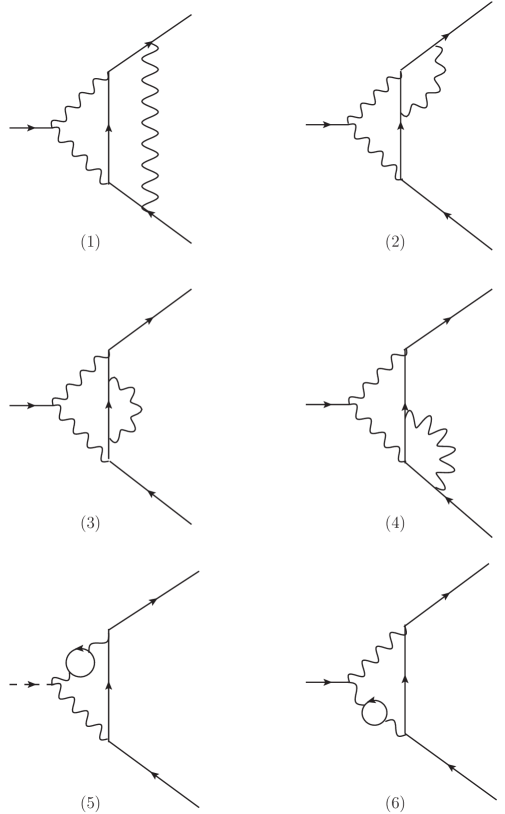
The aim of our paper is to present a more detailed analysis of the two-loop QED radiative corrections without using any approximation in order to check the validity of the previous approximative results. The natural formalism to treat the problem systematically is the Chiral perturbation theory (PT) [22, 23, 24] enriched by photons and leptons [25, 26]. The leading order amplitude which is within the chiral power counting has been calculated in [4] and the matching of the relevant low energy constant to the QCD in the leading order of the large expansion has been done in [6]. The next-to-leading order contributions have not been calculated within this formalism yet. They can be divided into two groups. The first group corresponds to the additional strong higher order corrections to the vertex with pions inside the loops and it counts as while the second one collects the pure QED corrections of the order . It is the latter group we will concentrate on in this paper. The relevant contributions consist of the six two-loop Feynman diagrams, namely the one box-type, two vertex-type, the electron self-energy insertion (these have been approximately investigated in [21]) and two vacuum polarization insertions. In order to renormalize the one-loop UV sub-divergences the corresponding one-loop counterterm diagrams have to be taken into account. Finally the remaining superficial UV divergence has to be renormalized by tree counterterm graph. The box-type diagram suffers further from the IR divergence, this is cancelled within the inclusive width.
In this paper we address the technical aspects of the calculation of the six two-loop Feynman diagram contributions mentioned above. The standard strategy consists of their reduction to the dimensionally regularized scalar integrals which will be subsequently expressed in terms of the eighteen Master Integrals. This can be done using the Laporta-Remiddi algorithm [27, 28] which is based on the integration by parts identities [29, 30] and Lorentz invariance identities [31]. We then calculate the Master Integrals using the technique of differential equations [32, 33, 34, 35, 36] and expand them up to and including the order (where ) in terms of the harmonic polylogarithms [37]. Some of the Master Integrals has been already published in the existing literature, we either take them over [38, 39] or make independent calculations in alternative bases within individual topology classes and afterwards check the results [40, 41, 42, 43, 44, 45, 46]. This re-calculation found agreement with the formulae published earlier. We have also added new yet unpublished parts of some of the Master Integrals (typically the terms of their expansion) in the closed form for the first time. We also discuss in detail the aspects of the UV renormalization of the two-loop graphs including the counterterm graphs described above and the treatment of the IR divergences within the soft-photon approximation. We give also the numerical analysis and discuss the various approximation to the exact two-loop expression.
The paper is organized as follows. In Section 2 we summarize our notation and discuss the general structure of the amplitude. The third section is devoted to the general aspects of the systematic chiral expansion of the amplitude. Here we also give a list of the two-loop and one-loop Feynman diagrams contributing to the next-to-leading order pure QED corrections. In Section 4 we discuss the general strategy of the renormalization of the one-loop and two-loop contributions and the treatment of IR divergences within dimensional regularization in detail. Section 5 is devoted to the calculation of the one-loop graphs with one one-loop counterterm vertex and also our renormalization scheme is specified there. In Section 6 we calculate the two-loop graphs and in Section 7 we discuss the soft-photon bremsstrahlung. In Section 8 we put all the ingredients together and give the final result for the virtual and real QED radiative corrections. We also discuss large logarithm approximation and relate our result to the Bergström’s calculation. Some preliminary phenomenological applications are discussed in Section 9. In Section 10 we give a brief summary and conclusion. Some technical details are postponed to the Appendices. The relevant part of the Lagrangian with virtual photons and leptons is summarized in Appendix A. The reduction of the six two-loop graphs to the scalar integrals is presented in Appendix B. In Appendix C we list the integration-by-parts identities for the scalar integrals and in Appendix D we summarize the results of our (re-)calculation of the relevant Master Integrals and give a comparison with existing literature.
2 Basic properties of the amplitude
In this section we discuss the basic features of the amplitude. We set the notation and kinematics and then briefly comment on the general properties of the lowest order amplitude which corresponds to order in electromagnetic interaction (and all orders in QCD for the pion transition form factor, which is here the only nonperturbative ingredient).
2.1 Notation and kinematics
The invariant amplitude for the decay is defined by means of the matrix element
| (2.1) |
which is supposed to be calculated in the presence of strong and electromagnetic interactions. According to the Lorentz covariance we can further write
| (2.2) |
where is a one particle irreducible vertex. Off shell it can be conveniently decomposed introducing four scalar form factors , and defined as111In what follows we use the convention and .
| (2.3) |
Here and the charge conjugation invariance implies
| (2.4) |
For the electron-positron pair on shell we get then
| (2.5) |
and, as a consequence, the total decay rate is given solely in terms of the on-shell form factor as
| (2.6) |
where
| (2.7) |
is the velocity of the electron-positron pair in the CM frame.
Note that the semi-on-shell form factor can be extracted from the one particle irreducible vertex by means of the following projection
| (2.8) |
This dimensionless form factor is an analytical function of the variable in the complex plain with a cut where the unphysical threshold corresponds to the two-photon intermediate state. For further convenience we introduce two dimensionless kinematical variables, namely
| (2.9) |
and
| (2.10) |
which map the unphysical threshold to and respectively.
In what follows we assume perturbative expansion of the amplitude in the QED coupling . Consequently we can write for the form factor
| (2.11) |
where and , and for the decay rate
| (2.12) |
In order to cancel the infra red (IR) divergences present in we have to add also the real photon bremsstrahlung contribution and consider inclusive decay rate of the process222Note that the same final state has also the Dalitz decay , which is however dominant in different region of the phase space corresponding to small (cf. (1.2)). For large enough the Dalitz decay contribution is tiny, however, for the experimentally used cut on this contribution should be also included. . The size of the NLO real and virtual QED radiative corrections can be then described by means of the factor defined as
| (2.13) |
where is the Dalitz variable (1.2) and where all the events with are included.
2.2 The amplitude at the order
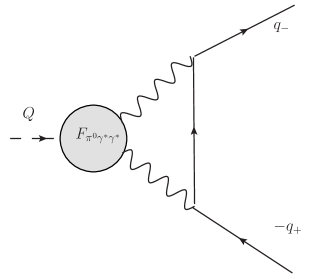
Within the QED the leading order contribution to is of the order and comes from the diagram depicted in Fig. 1. The bubble there corresponds to the strong matrix element
| (2.14) |
where is the hadronic part of the electromagnetic current
| (2.15) |
and is the pion transition form factor.
The explicit formula reads then
| (2.16) | |||||
and using the projection (2.8) we get (cf. [47])
| (2.17) |
where we abbreviated
| (2.18) | ||||
| (2.19) |
and where
| (2.20) |
is the triangle function.
The pion transition form factor represents the unknown nonperturbative QCD ingredient of the above formula, therefore the evaluation of the integral (2.17) is model dependent. However some general features of (2.17) can be deduced in a model independent way. We will discuss them in the rest of this section.
Let us first briefly remind the properties of . It has the following short distance asymptotics which is a consequence of OPE. For fixed and we have [48] (see also [7])
| (2.21) |
(where is the pion decay constant) and therefore we can conclude that the integrals (2.16) and (2.17) are convergent. Also the long distance asymptotics of is known from the first principles being fixed by the QCD chiral anomaly. Namely in the chiral limit
| (2.22) |
and therefore the low energy behavior is expected to be given by the chiral expansion of the form
| (2.23) |
where is the hadronic scale limiting the applicability of .
Another useful model independent property is that the two-photon intermediate state contribution to the imaginary part of the leading order form factor (2.17) with extended off the pion mass shell333Note that can be obtained by means of the LSZ reduction formula from the three-point correlator [6] where is the pseudoscalar density. Namely for we have This offers the natural possibility to extend the form factor off the mass shell is uniquely fixed by the value . Indeed, using the Cutkosky rules and cutting the two internal photon lines we get [1],[2]
| (2.24) |
For this contribution saturates the imaginary part of . As a consequence, the known imaginary part and the known width of the pion decay in the leading order in the QED expansion,
| (2.25) |
can be further used to get another exact result concerning the branching ratio
| (2.26) |
Namely, using instead of in (2.6), we get the following model independent unitarity bound [2]
| (2.27) |
The explicit knowledge of allows also to pinpoint the most important nonanalytic contribution to , namely that stemming from the two-photon intermediate state. The latter is given by means of the following once subtracted dispersive representation [3]
| (2.28) |
and it is therefore fixed uniquely up to one unknown subtraction constant . The dispersion integral for the physically relevant region reads
| (2.29) |
In this formula is given by (2.10) and is the dilogarithm defined as
| (2.30) |
which is analytic in the complex plain with cut . The unknown explicit form of the form factor in the intermediate energy region can influence only the subtraction constant .
As a consequence, we can split the leading order amplitude into two parts, namely
| (2.31) | |||||
The first part corresponding to the two photon intermediate state is completely independent on the details of the pion transition formfactor. The second part (where is an intrinsic scale characteristic for the formfactor , i.e. the scale at which is the integral (2.17) effectively cut off) accumulates the above subtraction constant as well as the contributions of higher intermediate states which appear when also the bubble in the Fig. 1 is cut. The explicit form of the as a functional of unknown transition formfactor has been derived in [18] with use of the Mellin-Barnes representation.
We have explicitly kept apart the logarithmic term in the square brackets of (2.31). The reason is that this term corresponds to the leading dependence of on the effective cut-off scale . The origin of this term is easy to understand [3]. In the case of point-like pion (i.e. when ), the integral (2.17) is logarithmically divergent. Using the sharp cut-off at the scale instead of effective cut-off provided by we get for
| (2.32) |
where the part includes terms that are finite or suppressed for . Thus we expect the same behavior also for the full amplitude and therefore for .
Because the discontinuities of as a function of start at , is analytic in the physical region and can be therefore expanded in this region in the power series of the variable . This suggests that can be approximated at the leading order of this expansion by -independent constant.
3 Systematic chiral expansion
Within the variant of supplemented with dynamical photons and electrons (cf. [26]) the formfactor is given in terms of the systematic simultaneous expansion in powers of the momenta (), the quark and electron masses and the fine structure constant , to which the chiral orders are formally assigned according to
| (3.1) |
The relevant parts of the enlarged Lagrangian are listed in the Appendix A. The hierarchy of the various contributions is then controlled by the Weinberg power-counting formula [22]. As is usual in , for the regularization of UV as well as IR divergences we use the dimensional regularization (DR) in what follows. In order to avoid problems with intrinsically four-dimensional objects like Levi-Civita pseudo-tensor and we use here the variant known as Dimensional Reduction. For calculation of this means that we first project out the form factor from the amplitude by means of (2.8) using four-dimensional Dirac algebra and only then we dimensionally regularize the resulting scalar integrals.
3.1 The leading order of the chiral expansion

The leading order contribution represents the chiral order444Note, that for the amplitude we have , because the fermion wave functions are counted as . and can be divided into two parts (see Fig. 2). The first one is a logarithmically divergent one-loop graph with local vertex stemming form the Wess-Zumino-Witten Lagrangian (here and in what follows we write down only the relevant vertices)
| (3.2) |
( is the pion decay constant in the chiral limit) and the second one corresponds to a tree-level counterterm graph originating in the Lagrangian
| (3.3) |
where is a renormalized counterterm coupling at a scale . One can think of the loop part of as approximating the leading order formfactor given by (2.17) by means of inserting the leading order term of the chiral expansion of the pion transition formfactor (2.23) into (2.17). This insertion however modifies significantly the high energy region of the loop integration starting at the onset of the resonances where the chiral expansion fails to converge. Such a modification of the loop has to be compensated by local counterterm contribution in such a way that the term of the chiral expansion of the is exactly reproduced. This is the general idea of the matching of the coupling constant . In the absence of the first principle determination of this matching procedure is however model dependent. We use here the value
| (3.4) |
which has been obtained in [6] by means of using a large inspired Lowest Meson Dominance (LMD) ansatz for .
As a result we get555At this order we can put . In fact, such a replacement corresponds to partial re-summation of the higher order corrections, namely the renormalization of the pion external leg.
| (3.5) | |||||
The structure of this expression can be easily understood. It corresponds to the formula (2.31) where both and have been replaced with the leading terms of their chiral expansion, provided we identify the renormalization scale with the intrinsic cut-off scale of the formfactor .
3.2 The part of the next-to-leading order
At the next-to-leading order the amplitude is generically in terms of the simultaneous expansion according to the chiral order assignment (3.1). At this order there are two types of contributions, which counts either as or as for the amplitude (or and for the form factor ). The contributions of the first type collect two-loop and one-loop graphs with the same topology as depicted in the Fig. 1 (where now the blob represents either a one loop subgraph with pion internal lines or order counterterm) and in addition tree graphs with counterterms666Strictly speaking there is also contribution from the pion external leg renormalization, which we have however effectively added in the LO by means of the replacement .. Such contributions can be understood as was mentioned above as the next-to-leading terms of the chiral expansion of (2.31).
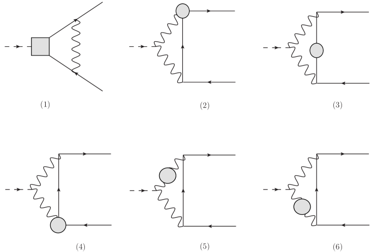
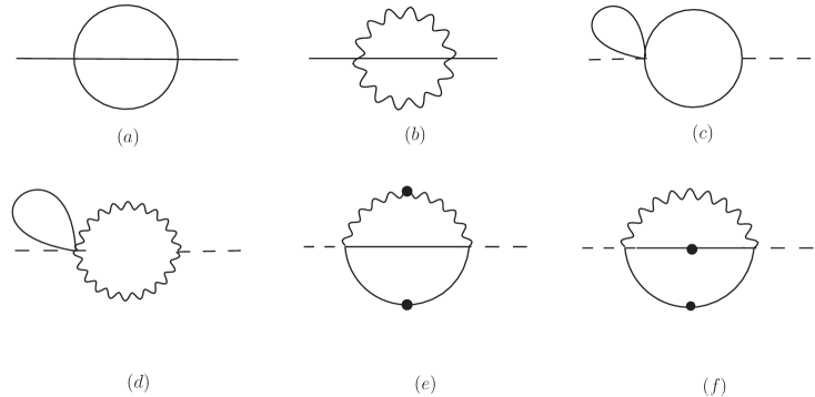
In this paper we will concentrate on the contributions of the second type (i.e ) which represent the pure QED corrections. In this case we get again three classes of graphs, namely six two-loops graphs with virtual photons and electrons (see Fig. 3), six one-loop graphs with counterterms (see Fig. 4, graphs (2)-(6)) or counterterm (see Fig. 4, graph (1)) which renormalize the one-loop subdivergences of the corresponding two-loop graphs and tree-level graphs which are necessary to renormalize the remaining superficial divergences. The latter are of the same order in as the counterterm (3.3) and therefore the relevant vertex from the Lagrangian can be summarily written in the form
| (3.6) |
where is the renormalized coupling and we have not written the UV divergent part explicitly.
4 Structure of the two-loop corrections and renormalization
In this section we briefly discuss the general structure of the one and two-loop contributions within the dimensional regularization and within renormalization scheme suitable for power counting non-renormalizable effective field theories [49] (cf. also [50]). This discussion will be helpful for the organization of the results of the explicit calculation and for consistency checks of the results presented in the next sections.
Let us write the effective Lagrangian in the form
| (4.1) |
where accumulates the counterterms which are needed in order to renormalize the superficial divergences of the loop graphs and is the dimensional regularization scale. Schematically
| (4.2) |
where are the renormalized counterterm couplings (i.e. the finite parts of the counterterms at the loop level) and is a set of operators. In the above formula for the factor naturally appears when the scale is artificially introduced into each loop integration writing in order to restore the four-dimensional canonical dimension of the dimensional integration measure.
4.1 Renormalization of the one-loop contributions
For the total one-loop contributions to any one-particle irreducible vertex entering the game we can write schematically
| (4.3) | |||||
where is the (four-dimensional) canonical dimension of . In this formula the first line represents the result of the loops while the second line accumulates the counterterm contributions. In this notation, both and are generally polynomials in the external momenta. Moreover is linear in the renormalized counterterm couplings introduced above. On the other hand, the functions for have more complicated analytical structure with branch points and cuts. In general, depend nonlinearly on the tree-level couplings . The chosen normalization ensures that are dimensionless. The above structure (4.3) is shared by the LO contribution to the formfactor and also by the UV divergent one-loop subgraphs of the NLO corrections to , namely the off-shell one-loop and vertices, the electron self-energy and the vacuum polarization.
We use here the renormalization scheme suitable for power-counting nonrenormalizable effective theories [49] and require renormalization scale independence order by order in the loop expansion. For this means that the following finite quantity
| (4.4) | |||||
has to be independent. This implies a running of according to
| (4.5) |
and corresponding running of the (linear combinations of ) counterterm couplings . As a result, (4.3) can be re-organized in the following simple manifestly RG invariant form
| (4.6) |
4.2 Renormalization of the two-loop contributions
For simplicity let us first assume that there are no infrared (IR) divergences. The generalization with the presence of IR divergences will be discussed in the next subsection.
At the two loop level, we have three types of contributions, namely
| (4.7) |
The first one corresponds the genuine two-loop contribution which can be schematically written in the form
| (4.8) |
The second one represents a sum of one-loop graphs with one-loop level counterterms which are necessary to renormalize the subdivergences of the two-loop part
| (4.9) | |||||
where we have explicitly pulled out the dependence on the renormalized one-loop counterterm couplings and coefficient of the corresponding infinite parts . Finally we have also a tree level contribution of the counterterms necessary to renormalize the remaining superficial divergence of , naively
| (4.10) | |||||
(here is polynomial in external momenta and linear combination of the couplings from ). However, in the absence of the IR divergences, in the sum only the local (i.e. polynomial in the masses and external momenta) UV divergences survive. This fact implies nontrivial relations between various , and which can be used either in order to simplify the above contributions or as a nontrivial check of the explicit calculations. Cancellation of the explicitly independent nonlocal terms in the sum needs (note that has to be local because it corresponds to the UV divergence of the one-loop graph)
| (4.11) |
where is local. Similarly, cancellation of the nonlocal terms proportional to requires
| (4.12) |
In fact these relations are valid also graph by graph. Introducing RG invariant counterterm couplings according to (4.4), namely
| (4.13) |
we can write using (4.11) and (4.12)
| (4.14) | |||||
and the remaining tree-level contribution coming from the two-loop counterterm can be then simplified as
| (4.15) |
Here the UV finite and RG invariant777As in the previous subsection we require RG scale invariance order by order in the loop expansion. We also tacitly assume that all the relevant contributions are included in which represents a RG invariant physical observable. local quantity is a two-loop analog of
| (4.16) | |||||
This implies the following explicit dependence of on the renormalization scale :
| (4.17) |
As a result we get the following simple and manifestly RG invariant form of the total two-loop contribution to :
| (4.18) |
4.3 Treatment of IR divergences
The presence of the IR divergences complicates the above simple picture a bit. After the UV divergences are subtracted, additional divergent terms survive, generally both in and , namely
| (4.19) |
and
| (4.20) | |||||
However, in the sum of these two contributions, the part has to vanish. This gives another useful relation which can be used as nontrivial check of the explicit calculation, namely
| (4.21) |
and we get for the remaining IR divergent part
| (4.22) |
In our case the only one one-loop counterterm graph with IR divergence is that corresponding to the counterterm of the vertex graph (let us denote the corresponding as in what follows) and in (4.22) the only relevant we denote as . The IR divergences in where
| (4.23) |
can be cancelled to the given order including the soft bremsstrahlung contribution into the inclusive decay rate, where
| (4.24) |
and where is a dimensionally regularized phase space bremsstrahlung integral (see Section 7) with a general structure
| (4.25) |
It holds schematically
| (4.26) |
Inserting (4.6) and (4.22) into (4.26) and collecting the coefficients at various powers of in the term gives the following conditions
| (4.27) |
and
| (4.28) | |||||
| (4.29) |
The latter two relations can be rewritten with help of (4.27) as
| (4.30) |
which represents another relation which can be used as a check of the explicit results. Using these relations, we get finally
which is manifestly independent on the RG scale .
5 The one-loop graphs
In this section we summarize the results for the one-loop graphs which are relevant for the full two-loop calculation. First we will present the one-loop contribution to the form factor in more detail including also the order which will be necessary for treating the IR divergences. We will also discuss the one-loop UV divergent subgraphs of the two-loop graphs and one-loop graphs with one counterterm vertex. We will explicitly point out the individual orders in according to the general structure discussed in the previous section. In order to simplify the results and to avoid some repeating multiplicative factors, we will present all the results in terms of the re-scaled form factor defined as
| (5.1) |
5.1 The leading order amplitude revisited
As we have seen from the general formula (LABEL:general_form_P), we need more detailed information on expansion of the LO amplitude (namely the term). In order to be consistent with the two-loop calculations it is also convenient to rewrite in terms of the Harmonic Polylogarithms of Remiddi and Vermaseren [37]. Let us note that in the physical region the kinematical variable is negative (cf. (2.10)), while the two-loop integrals are originally calculated in their analyticity region corresponding to and only then analytically continued (cf. Appendix D ). This continuation apart from generating imaginary parts brings about also additional minus signs into the arguments of Harmonic Polylogarithms and therefore the most convenient way how to present the result in the physical region is to use as an argument of these functions a new variable
| (5.2) |
In order to further simplify the long expressions we use the notation
| (5.3) |
and rewrite the rational function multiplying the Harmonic Polylogarithms in terms of the variable .
As a result we get then for the one-loop contribution (cf. Section 4 )
| (5.4) |
In the above formula (5.4) we have for
| (5.5) |
and the term is
where
For further convenience let us also mention explicitly the UV divergent part
| (5.8) |
The formula (3.5) can be then easily reconstructed as
| (5.9) |
and we can interpret the renormalization scale independent constant in terms of the renormalized constant at scale as
| (5.10) |
numerically
| (5.11) |
5.2 The one loop counterterms
In this subsection we summarize the counterterms needed for renormalization of the one-loop sub-divergences of the two-loop graphs. We can write the relevant counterterm Lagrangian in the general form either in terms of the renormalized couplings (finite parts of the counterterms)
| (5.12) |
(here ) or in terms of the renormalization scale invariant constants (cf. (4.4))
| (5.13) |
These counterterms contribute to the electron self-energy , the vertex function and vacuum polarization which are related to the physical electron mass and physical charge, namely
| (5.14) | |||||
| (5.15) |
Within our regularization scheme and at one-loop level we get
| (5.16) | |||||
| (5.17) |
therefore adjusting
| (5.18) | |||||
| (5.19) |
(i.e. choosing the on mass shell renormalization scheme) we ensure, that the original parameters and coincide with the physical mass and charge. The parameter is connected with the electron wave function renormalization, namely
| (5.20) |
where in our scheme at one loop (here the pole corresponds to the IR divergence)
| (5.21) |
Therefore the parameter is not physical and has to cancel in the physical amplitudes. We can conveniently set
| (5.22) |
then the only effect of the electron wave function renormalization is the IR pole which is cancelled by the analogous pole in the diagonal part of the bremsstrahlung integrals (see Section 7). We can therefore forget the electron wave function renormalization completely provided we simultaneously throw away the IR divergent part of the diagonal bremsstrahlung integrals.
5.3 One-loop graphs with counterterms
There are six types of the one-loop graphs with and counterterms which are depicted as in Fig. 4. Let us denote their individual contributions as . As a consequence of the symmetries of the graphs we have the relations
| (5.23) | |||||
| (5.24) |
and as a result of straightforward algebra we find that and are simply related to (cf. (5.4) and (5.8)), namely
Also can be rewritten in the form
| (5.26) | |||||
where formally corresponds to the topology of Fig. 4, but now with the insertion only of the modified mass counterterm
| (5.27) |
The only nontrivial one-loop graphs with counterterms are therefore and . The first one can be written as
| (5.28) |
where we have explicitly pointed out the IR divergent part. The individual orders of the expansion are then
| (5.31) | |||||
| (5.32) | |||||
For we get
| (5.33) |
where
| (5.36) | |||||
6 The two-loop graphs
This section is devoted to the six two-loop graphs depicted in Fig. 3. Let us denote their contributions to the re-scaled form factor defined by (5.1) as . Due to the symmetries of the graphs, we get the relations
| (6.1) | |||||
| (6.2) |
We have therefore only four independent two-loop contributions to the form factor . For their determination we use the standard procedure based on the reduction to the scalar Master Integrals (MI) and on calculation of the latter by means of the differential equations technique.
6.1 Reduction to Master Integrals
As a first step we define set of basic scalar integrals
| (6.3) |
where are integers and is a set of seven independent propagator denominators, namely
| (6.4) |
which at the same time form the basis for the seven independent scalar products build from the four-vectors , , and . The momentum flow in corresponds to the auxiliary diagram shown in Fig. 5. The integrals depend besides the electron mass only on one independent scalar variable and as a consequence of the symmetry properties of the auxiliary diagram they satisfy the relation
| (6.5) |
Note also, that some of are identically equal to zero. For instance whenever for (or ) simultaneously, we can factor out a massless tadpole and therefore vanishes.
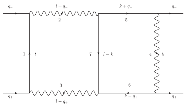
Using the projection (2.8) and expressing the scalar products in the numerator of the integrands in terms of we get schematically
| (6.6) |
where are known coefficients which depend on the variable and electron mass . The explicit form of the reduction formulae (6.6) can be found in the Appendix B. The relations (6.2) can be explicitly verified for the right hand side of (6.6) using (6.5).
There are altogether 172 integrals entering the sums in the reduction formulae (6.6), however, not all of them are independent. In addition to the symmetry property (6.5) there are also additional relations based on the integration by parts (IBP) [29, 30] and Lorentz invariance identities (LI) [31]. The former relations are consequences of the vanishing of the integral of the total divergence within DR. In our case we get eight relations schematically written as
| (6.7) |
The remaining LI relations express the invariance of the scalar integrals with respect to the Lorentz transformation of the external momenta
| (6.8) |
The left hand sides of both (6.7) and (6.8) (when contracted with ) can be expressed in terms of linear combinations of with various and with dependent coefficients. The explicit form of the resulting relations is postponed to Appendix C, here we give only the LI identity as an illustration:
| (6.9) |
where we have introduced the usual operators () which act on as
| (6.10) |
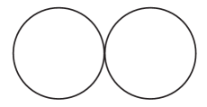
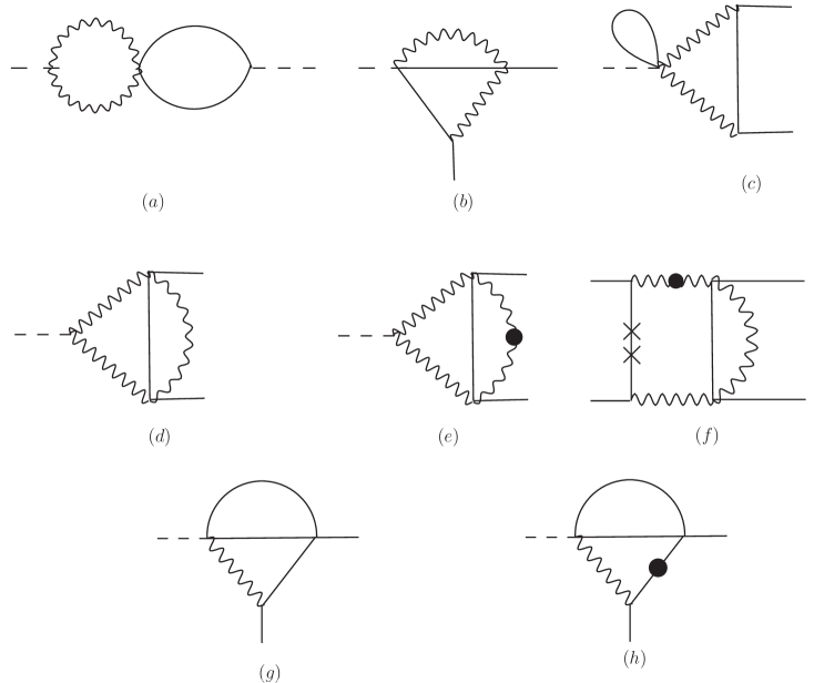
The above linear relations (6.7) and (6.8) together with the symmetry property (6.5) can be used as an input for the Laporta-Remiddi algorithm [27, 28] which allows further reduction of the number of the scalar integrals expressing them in terms of smaller number of MI. We have used the Maple implementation of the reduction procedure AIR [51] and found that all the necessary 172 integrals can be expressed in terms of 18 MI which belong to 12 different types of topologies, namely one two propagator MI (Fig. 6, one topology), six three propagator MI (Fig. 7, five topologies), eight four propagator MI (Fig. 8, five topologies) and three five propagator MI (Fig. 9, two topologies). In the above figures, the dots added to the internal propagator line mean that corresponding (number of dots is ) while crossed line indicates that , i.e. the th propagator is missing and the integral is a tensor one (number of crosses corresponds to ). The set of MI is summarized in Tab. 1.

| Number of propagators | MI |
|---|---|
| 2 | |
| 3 | |
| 4 | |
| 5 |
As a final result of the reduction procedure we get the individual two-loop contributions in the form of linear combinations of the MI with dependent coefficients
| (6.11) | |||||
| (6.13) | |||||
According to the above formulae we shall need the MI up to (and including) the order . However, for the calculation of MI as described in the next subsection we need some of them to the order .
6.2 Calculation of the Master Integrals
Some of the MI are not genuine two-loop integrals and can be calculated simply as a product of one-loop integrals. This concerns four MI denoted by star in Tab. 1. The remaining fourteen MI can be obtained in a standard way as a solution of the appropriate closed system of ordinary linear differential equations [32, 33, 34, 35, 36]. The latter can be obtained by means of differentiating the integrals with respect to . On one hand, the result of such a differentiation contracted with external momenta can be related to the derivative of with respect to the variable as
| (6.15) | |||||
(here the second identity is a consequence of the LI). On the other hand, the right hand side of (6.15) can be expressed as a linear combination (with dependent coefficients) of the integrals belonging either to the same topology class or to the topologies with less propagators. Finally we get (in terms of the operators (6.10))888It is easy to see that the difference of both possible right hand sides of (6.16) just corresponds to the LI identity (6.9).
| (6.16) | |||||
Writing these equations for the MI we get at the right hand side along with the original MI also other ’s which can be subsequently expressed in terms of the MI to close the system. From the form of (6.16) it can be seen that the resulting set of differential equations has “triangular structure” in the sense that it connects the derivative of given MI either with MI with the same topology or with topologies with smaller number of propagators.
For further convenience we introduce dimensionless quantities defined as
| (6.17) |
and rewrite the differential equation for in terms of the variable (cf. (2.10)). The system (6.16) for is then solved order by order in the expansion writing
| (6.18) |
and expanding the right hand side of (6.16) to the given power of . At each order, we solve the corresponding equations in the unphysical region where the MI are analytic. The solution is then fixed uniquely up to the integration constants which can be determined by the requirement of the absence of singularities in some appropriately chosen points of this analyticity region. For the calculation we have used the Mathematica package HPL [52, 53]. The results are summarized in Appendix D where also comparison of our independent calculations with those existing in the literature is given.
6.3 Two-loop contributions
Inserting the results of Appendix D in formulae (6.11-LABEL:gamma_vac_pol_red) we obtain the final form of the two-loop contributions. Writing them in the form (cf. (4.8))
| (6.19) |
we get
| (6.20) | |||||
| (6.21) | |||||
| (6.22) | |||||
| (6.23) | |||||
| (6.24) | |||||
| (6.25) | |||||
| (6.26) | |||||
| (6.27) | |||||
| (6.28) | |||||
| (6.29) | |||||
| (6.30) | |||||
| (6.31) | |||||
The graph has beside the UV also IR divergences, which can be identified using the general identities from Subsection 4.3. We get for ,
| (6.32) |
where
| (6.33) | |||||
| (6.34) | |||||
| (6.35) | |||||
| (6.36) | |||||
From the above formulae the general relations (4.12), which are valid for each graph separately, can be easily verified.
6.4 Two-loop counterterm contribution
For the construction of the two-loop counterterm (3.6) we need further the local parts of the UV divergences of the two-loop graphs (cf. (4.11)). Using the results of the previous (sub)sections we get
| (6.37) |
where are the coefficients of the UV divergent parts of the one-loop (sub)graphs (see (4.3)). According to general formula (4.15) we get for the two-loop counterterm contribution
| (6.38) | |||||
and for our choice of the renormalization scheme
| (6.39) |
where
| (6.40) |
To get the numerical values of the two-loop radiative corrections, we need to know the NLO counterterm coupling or its scale dependent renormalized value . In principle it can be obtained similarly as (cf. [6]) by means of matching of the (complete) NLO chiral expansion of the amplitude with the sum of the same types of graphs as we calculated but now with appropriate model of nonlocal off-shell pion transition form factor in place of the local vertex (3.2). This is however beyond the scope of our paper. Instead we make a simple estimate of the value of using its running with the renormalization scale. From (6.40) with central value of (see (5.11)) we get
| (6.41) |
We therefore roughly estimate
| (6.42) |
and get finally
| (6.43) |
7 Soft photon bremsstrahlung
Within the soft photon approximation, the amplitude of the process factorizes
| (7.1) |
where is the polarization vector of the emitted photon with soft momentum and helicity . Taking the square of the modulus, summing over helicities and integrating over the soft photon region defined by the experimental energy cut
| (7.2) |
we get
| (7.3) |
where
| (7.4) |
The latter integral is IR divergent and can be regularized using DR. Let us divide the resulting into the diagonal part
| (7.5) |
and non-diagonal part
| (7.6) |
In the rest system of the decaying pion both integrals are elementary and we get
| (7.7) | |||||
and
| (7.8) | |||||
Note that the IR divergent part of coincides up to a sign with that of the (see (5.21)). The latter factor is necessary for the renormalization of the external fermion lines. Namely, on the level of the decay width
| (7.9) |
As we have mentioned in Subsection 5.2, within our renormalization scheme
| (7.10) |
Therefore up to the assumed accuracy we can effectively make the following replacement
| (7.11) |
provided we replace with its finite part.
8 The two-loop radiative correction
8.1 The exact two-loop result
Putting the results of the previous sections together and using the general formula (LABEL:general_form_P) we can finally write for the complete QED two-loop correction (2.13) schematically
| (8.1) | |||||
In this formula and the variable is connected to the maximal energy of the soft photon included into the inclusive decay rate by (7.2). In the above expression we have explicitly separated the contribution coming from the bremsstrahlung, the RG invariant NLO coupling and the individual graphs:
| (8.2) | |||||
Here we have inserted for the particular values corresponding to our choice of the renormalization scheme (cf. Section 5.2) and , , , and are explicitly given in Subsections 6.3, 5.3 and 5.1 respectively.
The numerical results for various contributions are summarized in the second column of Tab. 2. Here we use for the constants and the values (5.11) and (6.43) and the following numerical entries: , and . For the sum of all the contributions we get finally
| (8.3) |
where as the only source of errors we take the uncertainties of and . We observe considerable cancellation between the large contributions and which makes the role of the relatively smaller contributions of the other graphs numerically important.
Adding the bremsstrahlung we have
| (8.4) |
and for which is the cut used by KTeV we get
| (8.5) |
8.2 Large-logarithm approximations to the exact result
The exact two-loop expressions for and for are rather long but they can be approximated with a very good accuracy performing the large-logarithm (LL) expansion in terms of
| (8.6) |
and taking into account only the leading terms (up to the order ). For the various contributions we get999In these and following formulae we omit also all the terms of the order .
| (8.12) | |||||
and
| (8.13) | |||||
| exact | LL, rational | LL, polynomial | LL, polynomial, RG | ||
|---|---|---|---|---|---|
Inserting the above expressions into (8.1) we get an approximation of in terms of the rational function of the variable . It would be tempting to expand further the factor in (8.1) and approximate the whole as a second order polynomial of with the result
| (8.14) |
or numerically
| (8.15) |
and
| (8.16) |
We can also proceed apparently more carefully and include part of the large RG logarithms into the expansion writing ; such a modification makes a difference in the terms of the expansion. We get in this case101010In the final expression we expressed again and in terms of and .
| (8.17) | |||||
which gives
| (8.18) |
In both cases the reason for not very good agreement with the exact result is that the expansion of does not converge well111111While , the approximation up to the order gives . Including part of the large RG logarithms into the expansion as described in the main text we get and therefore it is much safer to approximate in terms of rational function of . We have compared all the possibilities (LL rational, LL polynomial and LL polynomial with RG logs included) in the third, fourth and fifth column of Tab. 2 respectively. The rational LL approximation is in excellent agreement with the exact result.
The LL approximation was originally calculated by Dorokhov et al. in [21] including only the graphs (1)-(4) in the Fig. 3 and taking into account only selected regions of the two-loop integration space. As we know from (8.12), the omitted graphs contribute only in the next to leading order in the LL expansion, however due to the accidental cancellation of the leading order terms they are in fact numerically important. The result of [21] for the virtual and soft photon corrections is
which numerically gives for a correction with significantly larger absolute value in comparison with (8.5),
| (8.20) |
The formula (LABEL:delta_Dorokhov) could be compared with our polynomial LL approximations after subtracting the contributions of the graphs (5) and (6) in Fig. 3 (i.e. those with vacuum polarization insertion into the internal photon lines). In the two variants described above we get however a result substantially different from , namely
| (8.21) |
and
| (8.22) |
and numerical values for
| (8.23) | |||||
| (8.24) |
The reason of this discrepancy is difficult to trace out because a completely different framework has been used for the calculations in [21] and we therefore left this problem open for further study.
8.3 Point-like vertex approximation
Let us briefly comment on another type of approximation which is connected with the model calculation of the QED radiative corrections by Bergström [12]. His result including virtual corrections and soft photon bremsstrahlung reads
| (8.25) |
where the terms, which we do not write explicitly, stem from the fact that the real photon radiation was calculated exactly i.e. beyond the soft photon approximation. Taking also these terms into account we get numerically
| (8.26) |
which is remarkably close to (8.20). However, the calculations [12] used a completely different approximation from the LL one that was used in [21].
In the paper [12] the approximation was based on the substitution for the nonlocal one-loop (sub)graph with a local effective vertex of the form
| (8.27) |
In appropriate renormalization scheme this vertex is essentially equivalent121212We ignore here the axial anomaly which does not contribute to the relevant matrix element. to the vertex
| (8.28) |
which takes properly into account the GB nature of pion and has the same structure as the counterterm (3.3). The Bergström’s calculation can be therefore qualitatively understood as the leading order term in the formal large expansion of the full two-loop result 131313Note that in the limit only the contribution of the one-loop graph (1) of Fig. 4 and soft bremsstrahlung are effectively taken into account. (i.e. corresponding to the assumption of small nonlocal part of one-loop (sub)graph in reference to its local part represented by ). Performing further the LL expansion of this leading term we get for the Bergström-like approximation of our result141414The difference between (8.25) and (8.29) corresponds to different regularization of the IR divergences and different renormalization scheme.
| (8.29) |
For illustration purposes we add the corresponding numerical values as the sixth column of Tab. 2. However for physical value of such an expansion does not converge (note that ) and therefore the Bergström’s result can not be taken as a serious approximation of the full two-loop .
9 The phenomenological applications of the results: first look
In this section we discuss several issues connected with the phenomenological aspects of the results obtained above. Up to now we have fixed or estimated the free parameters and of the effective Lagrangian and concentrated on the corresponding prediction of the two-loop QED corrections. In such a way obtained represents a part of the theoretical tools necessary for a precise extraction of the from experimental data. Therefore a consistency check of our final result (which uses one specific value of ) with that using other estimates of which are available in the literature should be desirable. Such a check is the topic of the first subsection.
We can also, however, reverse the point of view and investigate the sensitivity of the theoretical prediction for the branching ratio on the free parameter and try to extract the information on its actual value from the experimental data. Though we have not all the necessary ingredients at hand, we can make a preliminary analysis of this issue. This is done in the second subsection.
Last but not least, our result is closely related to the calculation of two-loop QED corrections to the class of processes of the type where and ; this relation is briefly discussed in the last subsection.
| CLEO bound | CLEO+OPE | QCDsr | LMD+V | QM | NQM | VM | |
|---|---|---|---|---|---|---|---|
9.1 Note on the dependence on
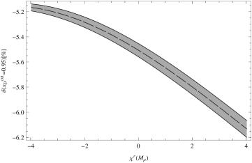
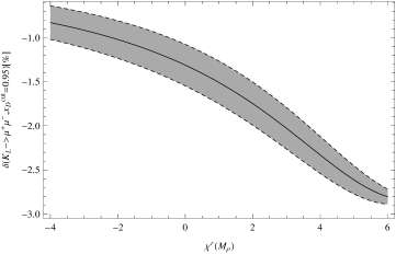
In the above numerical calculations we have fixed the value of the constant according to the large inspired LMD estimate (3.4) of the effective coupling entering the Lagrangian (3.3). In the literature there exist, however, further model dependent estimates of this constant based on various models or phenomenological parameterizations of the pion transition form factor (see [11] for comprehensive review). In Tab. 3 we summarize various values of and which we take over151515In [11], the values of are presented. from [11]. The first three columns (denoted as CLEO bound, CLEO+OPE and QCDsr) correspond to various treatments of the parametrization of using the CLEO [10] data (see [11] for details), next column (LMD+V) is the improvement of the large estimate mentioned above including two multiplets161616This ansatz is denoted gVMD in [11] [6]. The column QM is based on the constituent quark model while the last two columns (NQM and VM) on two variants of the nonlocal chiral quark model [54] and [55] respectively. In the the last row we illustrate the sensitivity of our result for the central value of on . All but the last resulting central values of are compatible with LMD result (8.5) within the estimated error bar. The dependence of on in a wider range is plotted in Fig. 10 where also the variation with inside its estimated error bar is illustrated by the filled band. 171717Note that for fixed the dependence of on is trivial (i.e. linear as can be seen from (8.1)).
9.2 Note on the phenomenological determination of from decay
Let us stress that the above analytical result for represents only a part of the problem of the complete QED radiative corrections to the process under consideration, and that the realistic analysis of the experimental data requires several additional pieces of information. The first one corresponds to the issue of the hard photon bremsstrahlung for which the soft photon approximation is not an adequate framework and for which more appropriate calculations have to be done. A closely related issue is the applicability of soft photon approximation for the KTeV choice of the cut . Another missing information is connected with the Dalitz decay which yields the same final state as the real photon bremsstrahlung in the decay. Though this process is dominated by low and is therefore suppressed for , its integrated contribution is known to grow rapidly with decreasing .
These additional issues have been addressed in the present context already in the paper [12], (see also [21]) and in this form they have been used for the analysis of the experimental data by the KTeV collaboration [8]. However, the analysis performed in [12] might be incomplete. As far as the hard photon bremsstrahlung is concerned, the point-like vertex approximation described in Subsection 8.3 has been used. This approach is, however, well justified only for the soft photon region where the details of the off-shell vertex are inessential.
Also, the corrections due to the Dalitz decay calculated in [12] (based on the radiative corrections to obtained in [56]) and used in [8] should be taken with some caution. As it has been shown recently [57], the one-photon irreducible () contributions which were omitted in [56] are in fact important already for where they give a negative contribution of the leading order differential decay rate .
The importance of the detailed knowledge of is twofold. On one hand, because the Dalitz decay has been used by KTeV-E799-II as a normalization and because the measured quantity was the ratio
| (9.1) |
it is necessary to extrapolate the Dalitz branching ratio to the full range of . As this extrapolation is concerned, the missing corrections to are in fact inessential, since the contribution of corrections integrated over the full phase space can be shown to be one order of magnitude smaller then the experimental error of the branching ratio (see [57] for details). On the other hand, has been used in order to subtract the Dalitz decay background in the region . Here the effect of missing contributions might be more important.
Let us give here only a preliminary illustration of the interrelation of our partial result of the QED radiative corrections and the precise branching ratio (1.1) obtained by KTeV-E799-II. Taking the above theoretical uncertainties into account we can write our prediction for the KTeV measured branching ratio as
| (9.2) | |||||
where the only experimental input is the precise branching ratio . In the above formula
| (9.3) |
is the difference between the soft photon and exact bremsstrahlung correction and
| (9.4) |
corresponds to the unsubtracted fraction of the Dalitz decay background discussed above. Without detailed knowledge of the exact bremsstrahlung we can only roughly estimate the error of the soft photon approximation with help of the point-like vertex approximation used in [12]. We get
| (9.5) |
which gives for a reasonable difference
| (9.6) |
As far as the unsubtracted fraction of the Dalitz decay background is concerned, we can use the explicite formulae for the corrections taken from [57] and arrive at181818Here we neglect a very weak dependence on the constant in the numerator.
| (9.7) |
which gives for
| (9.8) |
Note that both these additional contributions are larger then the variation of with inside its error bar (which yields ).
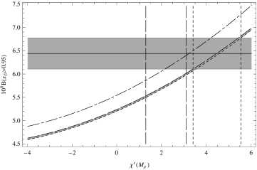
In the Fig. 11 we have plotted the right hand side of (9.2) as a function of both with and without the estimated additional contributions and together with the leading order branching ratio against the experimental value (1.1). The vertical bands correspond to the large inspired LMD estimate and to the range of values compatible with (1.1). These bands do not overlap, the preferred region of is shifted towards higher values191919Quite interestingly, even higher values of have been obtained from similar analysis of the related decays , namely or [58], and the bigger solution obtained from , namely [59]. Here the solution for shows two-fold ambiguity which is present also in the case, however we have fixed it keeping only the solution closer to the large prediction., namely which corresponds to .
9.3 Generalization to the decays

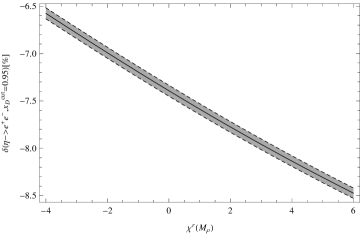

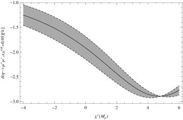

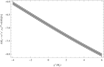

From the point of view of the coupling constant is universal202020The analogous statement is true also for ., because it enters the generalization of the counterterm Lagrangian given in Appendix A and is therefore connected with other processes of the type where and . These decays are governed at the leading order by the following effective long-distance Lagrangian
| (9.9) |
where is a normalization factor and is the effective long distance coupling which can be split into its universal and specific short-distance components
| (9.10) |
The latter is nontrivial only for the case where it is well known [60] , [61] (see also [59] and [62])
| (9.11) |
The Lagrangian is up to the normalization and shift in identical with that we have used for the calculation of the corrections to decay which means that our general result can be almost straightforwardly used for other processes by means of the substitution , and . More precisely, in such a way we obtain the contribution of the graphs depicted in Fig. 3 where all the fermion lines correspond to the final state lepton flavour, that means that for the decays we miss the vacuum polarization insertion graphs with electrons inside the loop. The results of such a generalization are illustrated in Tab. 4 where the corresponding corrections are listed (either for the same cutoff on the energy of the soft photon or at the same cutoff on ) and compared with the case of decay. To obtain these numbers we have fixed . As another illustration of the typical values of the (partial in the sense of the missing graphs) two-loop QED corrections we have plotted their and dependence in Figs. 12 and 13.
10 Summary and conclusion
In this paper we have calculated the two-loop QED radiative corrections to the rare decay including all the relevant graphs. As a result we have obtained exact analytical expression which takes into account the virtual photon contributions without any approximation. The IR divergences has been treated including real soft photon bremsstrahlung. The latter has been calculated within the soft photon approximation and added to the inclusive decay rate . We have worked in the framework of the with dynamical leptons and photons and parameterized the missing information on the details of the pion transition form factor in terms of two a priori unknown RG invariant couplings and which also incorporated the large RG logarithms. The numerical value of the first of these couplings has been obtained using the analysis of [6] based on the large matching and LMD ansatz, while the value of the second one (on the value of which our result proved to be much less sensitive) has been estimated from the running of the corresponding renormalized coupling with the RG scale .
The main motivation of our work was to test the validity of two approximative calculations of the QED radiative corrections already existing in the literature, namely the Bergström’s point-like (sub)graph approximation [12], which has been used for the analysis of the experimental data by the KTeV collaboration, and the more sophisticated large-log approximation [21] which claimed to confirm the applicability of the previous one.
We have identified the Bergström’s calculation as a leading term in the large expansion of the exact two-loop result. We have found that this expansion did not converge and therefore could not be trusted without reservation. The numerical discrepancy between the exact result and the Bergström’s one seems to confirm this conclusion.
Next we have discussed several variants of the LL approximations derived from the exact two-loop result. The two polynomial ones differ from the exact result by roughly twice the error estimated from the uncertainty of the couplings and while the rational one gives an excellent agreement. However we did not manage neither to confirm the LL calculation of [21] nor to reveal the reason of its large difference from our result. The approximation [21] was obtained in completely different framework and we therefore left the final resolution open to further studies.
Our final result numerically reads (see the definition (2.13))
| (10.1) |
and for the cut chosen by KTeV
| (10.2) |
Here the error stems from the uncertainty of and . Our result significantly differs from the previous approximative calculations [12, 21]
| (10.3) |
and the change is in the right direction towards the agreement of the experimental data with the SM prediction.
Let us note, that for the realistic analysis of the experimental data it is necessary to discuss carefully two further topics, which we have only partially included in this work, namely the real final state radiation beyond the soft photon approximation and the incorporation of the Dalitz decay contribution. The former is important because it is well known that the soft photon approximation is not much reliable except of very limited region in the phase space due to the small electron mass. The latter process, which has been recently revisited in [57], is known to yield a non-negligible background of roughly [12] near the cut chosen by KTeV. The more detailed analysis of these issues is still in progress. In this work we have performed only preliminary simplified analysis and found that the SM prediction for the branching ratio might be reconciled with the experimental value for , which is however off the predictions for based on the phenomenological models of the pion transition form factor.
Acknowledgement
We would like to thank Marc Knecht for initiating this project and for valuable discussions at the beginning and Karol Kampf for valuable discussions. This work is supported in part by Center for Particle Physics (project no. LC 527) of the Ministry of Education of the Czech Republic.
Appendix A The Lagrangian with dynamical photons and leptons
In this appendix we summarize the relevant parts of the Lagrangian with dynamical photons and leptons. Following the notation of [25] and using the variant of the theory (see also [63]) we need the following terms of the complete Lagrangian
| (A.1) |
where
| (A.2) |
and where
| (A.5) | |||||
| (A.6) | |||||
The coupling is connected with according to
| (A.7) |
Appendix B Reduction to scalar integrals
In this appendix we give the reduction of the individual two-loop graphs to 172 scalar integrals.
| (B.1) | |||||
| (B.2) | |||||
| (B.3) | |||||
| (B.4) | |||||
Appendix C The IBP identities
Here we list the IBP identities
| (C.1) |
where and , , . We present these identities in the form
| (C.2) |
where the operators corresponding to the insertion of into the loop integral can be rewritten in terms of the operators (6.10) as
| (C.3) |
Appendix D Results for Master Integrals
The results for MI are written in terms of the dimensionless quantities defined in (6.17).
D.1 Two propagator topology
This topology contains only one MI depicted in Fig. 14. It factorizes to one loop diagrams (i.e. a square of a tadpole) and hence can be computed straightforwardly.

We get the result
| (D.1) |
which has the following expansion
D.2 Three propagator topology, type a
There is a single MI in this topology, see Fig. 15 . It is independent thus can not be computed using the differential equations technique as formulated in this paper. Moreover, it does not factorize so the evaluation is more involved. However, the result can be found in the literature. The pioneering calculation was done in [38] as far as we know. It was further generalized in [39] and both results agree.

D.3 Three propagator topology, type b
This single Master integral depicted in Fig. 16 does not depend on and could be calculated directly using Feynman parametrization.

| (D.2) |
Expanding the above formula gives
D.4 Three propagator topology, type c
This topology includes one MI (see Fig. 17) and corresponds to the product of one-loop integrals. The expansion of the latter was studied in [40].

The convenient point for fixing the integration constants was in this case which is below the physical threshold. The solution is
We checked this MI with [43] where it is computed using the same formalism to including. Comparing the results gives an agreement.
D.5 Three propagator topology, type d
This MI depicted in Fig. 18 could be computed directly using loop integration (it factorizes to an off-shell massless bubble and a tadpole).

The result reads
| (D.3) |
and has the following expansion
Also this MI was checked with [42] and a complete match was reached.
D.6 Three propagator topology, type e
There are two nested MIs (see Fig. 19).
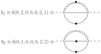
The suitable point for fixing the integration constants was chosen as . Then the solution reads
This pair of MIs belongs to the general class J011, the expansion of which was studied systematically in [40, 41]. In the framework of differential equations approach they were calculated in different basis across the literature [43, 44, 45]. We use the same basis as in [44] thus we verified their results to including.
D.7 Four propagator topology, type a
This topology includes the Master integral depicted in Fig. 20.

It is a product of a massive (see [40]) and a massless bubble. The former one can be easily extracted from and the latter one can be calculated directly. So we used this trick instead of solving the corresponding differential equation. The solution for current orders reads
Making a check with [42] up to lead to full agreement.
D.8 Four propagator topology, type b

D.9 Four propagator topology, type c
The third four propagator topology contains one Master integral depicted in Fig. 22

which has the following solution (integration constants fixed at )
We verified the result of [42] to .
D.10 Four propagator topology, type d
Our choice for the two Mater integrals in this topology is depicted in Fig. 23.
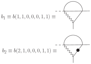
Here we tried two points for fixing the integration constants and both gave the same result. The expansion of the solution in powers of is
These Master integrals appear in [43] in the same basis. Making a check leads to complete agreement up to .
D.11 Four propagator topology, type e
This topology includes three coupled Master integrals , , . We make a transformation to a more suitable basis depicted in Fig. 24.
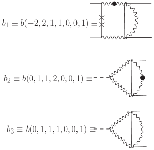
In this basis the system decouples and the solution may be found as in previous cases (using the point to fix the unknown integration constants)
The last two MIs and can be found in [42] in the same basis while for the first one we use a different basis. The former two were checked to and the latter one was left uncontrolled.
D.12 Five propagator topology, type a
The current topology is formed by the MI depicted in Fig. 25. It corresponds to F10101 of [40, 41] where the expansion was given.

This MI has the following expansion using for fixing the integration constants
Verifying the result with [42] to gave full agreement.
D.13 Five propagator topology, type b
We have chosen the two Master integrals as depicted in Fig. 26 (the AIR original basis was and ).
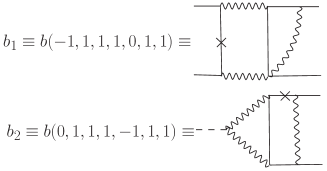
This choice has been done in order to decouple the system of corresponding differential equations. The appropriate point for fixing the integration constants was . Then it has the solution
This couple of MIs can be found in [46]. We performed a transformation to the original basis and made a check only for which exactly appears also in [46]. The result is in correspondence up to . However, this verifies both of our MIs since the transformation mixes them to . The above paper does not offer higher orders so we add them to the list of existing MIs.
References
- [1] S. Drell, “Direct decay ,” Nuovo Cim. XI (1959) 693.
- [2] S. Berman and D. Geffen, “The Electromagnetic Structure and Alternative Decay Modes of the ,” Nuovo Cim. 18 (1960) 1192.
- [3] L. Bergstrom, E. Masso, L. Ametller, and A. Bramon, “ Duality and Rare Pion Decays,” Phys. Lett. B126 (1983) 117.
- [4] M. J. Savage, M. E. Luke, and M. B. Wise, “The Rare decays , and in chiral perturbation theory,” Phys. Lett. B291 (1992) 481–483, arXiv:hep-ph/9207233.
- [5] L. Ametller, A. Bramon, and E. Masso, “The and decays revisited,” Phys. Rev. D48 (1993) 3388–3391, arXiv:hep-ph/9302304.
- [6] M. Knecht, S. Peris, M. Perrottet, and E. de Rafael, “Decay of pseudoscalars into lepton pairs and large QCD,” Phys. Rev. Lett. 83 (1999) 5230–5233, arXiv:hep-ph/9908283.
- [7] M. Knecht and A. Nyffeler, “Resonance estimates of low-energy constants and QCD short-distance constraints,” Eur. Phys. J. C21 (2001) 659–678, arXiv:hep-ph/0106034.
- [8] KTeV Collaboration, E. Abouzaid et al., “Measurement of the rare decay ,” Phys. Rev. D75 (2007) 012004, arXiv:hep-ex/0610072.
- [9] CELLO Collaboration, H. J. Behrend et al., “A Measurement of the , and electromagnetic form-factors,” Z. Phys. C49 (1991) 401–410.
- [10] CLEO Collaboration Collaboration, J. Gronberg et al., “Measurements of the meson - photon transition form-factors of light pseudoscalar mesons at large momentum transfer,” Phys.Rev. D57 (1998) 33–54, arXiv:hep-ex/9707031 [hep-ex].
- [11] A. E. Dorokhov and M. A. Ivanov, “Rare decay : Theory confronts KTeV data,” Phys.Rev. D75 (2007) 114007, arXiv:0704.3498 [hep-ph].
- [12] L. Bergstrom, “Radiative Corrections to Pseudoscalar Meson Decays,” Z. Phys. C20 (1983) 135.
- [13] Y. Kahn, M. Schmitt, and T. M. Tait, “Enhanced rare pion decays from a model of MeV dark matter,” Phys.Rev. D78 (2008) 115002, arXiv:0712.0007 [hep-ph].
- [14] A. Dorokhov, “Recent results on rare decay ,” Nucl.Phys.Proc.Suppl. 181-182 (2008) 37–41, arXiv:0805.0994 [hep-ph].
- [15] Q. Chang and Y.-D. Yang, “Rare decay as a sensitive probe of light CP-odd Higgs in NMSSM,” Phys.Lett. B676 (2009) 88–93, arXiv:0808.2933 [hep-ph].
- [16] D. McKeen, “Constraining Light Bosons with Radiative Upsilon(1S) Decays,” Phys.Rev. D79 (2009) 015007, arXiv:0809.4787 [hep-ph].
- [17] A. Dorokhov and M. Ivanov, “On mass corrections to the decays ,” JETP Lett. 87 (2008) 531–536, arXiv:0803.4493 [hep-ph].
- [18] A. Dorokhov, M. Ivanov, and S. Kovalenko, “Complete structure dependent analysis of the decay ,” Phys.Lett. B677 (2009) 145–149, arXiv:0903.4249 [hep-ph].
- [19] The BABAR Collaboration Collaboration, B. Aubert et al., “Measurement of the transition form factor,” Phys.Rev. D80 (2009) 052002, arXiv:0905.4778 [hep-ex].
- [20] A. Dorokhov, “How the recent BABAR data for affect the Standard Model predictions for the rare decays ,” JETP Lett. 91 (2010) 163–169, arXiv:0912.5278 [hep-ph].
- [21] A. Dorokhov, E. Kuraev, Y. Bystritskiy, and M. Secansky, “QED radiative corrections to the decay ,” Eur.Phys.J. C55 (2008) 193–198, arXiv:0801.2028 [hep-ph].
- [22] S. Weinberg, “Phenomenological Lagrangians,” Physica A96 (1979) 327.
- [23] J. Gasser and H. Leutwyler, “Chiral Perturbation Theory to One Loop,” Ann. Phys. 158 (1984) 142.
- [24] J. Gasser and H. Leutwyler, “Chiral Perturbation Theory: Expansions in the Mass of the Strange Quark,” Nucl. Phys. B250 (1985) 465.
- [25] R. Urech, “Virtual photons in chiral perturbation theory,” Nucl.Phys. B433 (1995) 234–254, arXiv:hep-ph/9405341 [hep-ph].
- [26] M. Knecht, H. Neufeld, H. Rupertsberger, and P. Talavera, “Chiral perturbation theory with virtual photons and leptons,” Eur.Phys.J. C12 (2000) 469–478, arXiv:hep-ph/9909284 [hep-ph].
- [27] S. Laporta and E. Remiddi, “The Analytical value of the electron at order in QED,” Phys.Lett. B379 (1996) 283–291, arXiv:hep-ph/9602417 [hep-ph].
- [28] S. Laporta, “High precision calculation of multiloop Feynman integrals by difference equations,” Int.J.Mod.Phys. A15 (2000) 5087–5159, arXiv:hep-ph/0102033 [hep-ph].
- [29] F. V. Tkachov, “A Theorem on Analytical Calculability of Four Loop Renormalization Group Functions,” Phys. Lett. B100 (1981) 65–68.
- [30] K. G. Chetyrkin and F. V. Tkachov, “Integration by Parts: The Algorithm to Calculate beta Functions in 4 Loops,” Nucl. Phys. B192 (1981) 159–204.
- [31] T. Gehrmann and E. Remiddi, “Differential equations for two loop four point functions,” Nucl.Phys. B580 (2000) 485–518, arXiv:hep-ph/9912329 [hep-ph].
- [32] A. V. Kotikov, “Differential equations method: New technique for massive Feynman diagrams calculation,” Phys. Lett. B254 (1991) 158–164.
- [33] A. V. Kotikov, “Differential equations method: The Calculation of vertex type Feynman diagrams,” Phys. Lett. B259 (1991) 314–322.
- [34] A. V. Kotikov, “Differential equation method: The Calculation of N point Feynman diagrams,” Phys. Lett. B267 (1991) 123–127.
- [35] E. Remiddi, “Differential equations for Feynman graph amplitudes,” Nuovo Cim. A110 (1997) 1435–1452, arXiv:hep-th/9711188 [hep-th].
- [36] M. Caffo, H. Czyz, S. Laporta, and E. Remiddi, “Master equations for master amplitudes,” Acta Phys.Polon. B29 (1998) 2627–2635, arXiv:hep-th/9807119 [hep-th].
- [37] E. Remiddi and J. Vermaseren, “Harmonic polylogarithms,” Int.J.Mod.Phys. A15 (2000) 725–754, arXiv:hep-ph/9905237 [hep-ph].
- [38] J. Fleischer, M. Y. Kalmykov, and A. V. Kotikov, “Two-loop self-energy master integrals on shell,” Phys. Lett. B462 (1999) 169–177, arXiv:hep-ph/9905249.
- [39] M. Argeri, P. Mastrolia, and E. Remiddi, “The Analytic value of the sunrise selfmass with two equal masses and the external invariant equal to the third squared mass,” Nucl.Phys. B631 (2002) 388–400, arXiv:hep-ph/0202123 [hep-ph].
- [40] A. I. Davydychev and M. Y. Kalmykov, “New results for the epsilon-expansion of certain one-, two- and three-loop Feynman diagrams,” Nucl. Phys. B605 (2001) 266–318, arXiv:hep-th/0012189.
- [41] A. I. Davydychev and M. Y. Kalmykov, “Massive Feynman diagrams and inverse binomial sums,” Nucl. Phys. B699 (2004) 3–64, arXiv:hep-th/0303162.
- [42] R. Bonciani, P. Mastrolia, and E. Remiddi, “Master integrals for the two loop QCD virtual corrections to the forward backward asymmetry,” Nucl.Phys. B690 (2004) 138–176, arXiv:hep-ph/0311145 [hep-ph].
- [43] R. Bonciani, P. Mastrolia, and E. Remiddi, “Vertex diagrams for the QED form-factors at the two loop level,” Nucl.Phys. B661 (2003) 289–343, arXiv:hep-ph/0301170 [hep-ph].
- [44] C. Anastasiou, S. Beerli, S. Bucherer, A. Daleo, and Z. Kunszt, “Two-loop amplitudes and master integrals for the production of a Higgs boson via a massive quark and a scalar-quark loop,” JHEP 0701 (2007) 082, arXiv:hep-ph/0611236 [hep-ph].
- [45] M. Czakon, J. Gluza, and T. Riemann, “Master integrals for massive two-loop bhabha scattering in QED,” Phys.Rev. D71 (2005) 073009, arXiv:hep-ph/0412164 [hep-ph].
- [46] M. Czakon, J. Gluza, and T. Riemann, “A Complete set of scalar master integrals for massive 2-loop Bhabha scattering: Where we are,” Nucl.Phys.Proc.Suppl. 135 (2004) 83–87, arXiv:hep-ph/0406203 [hep-ph].
- [47] L. Bergstrom, “Rare Decay of a Pseudoscalar Meson into a Lepton Pair: A Way to Detect New Iinteractions?,” Zeit. Phys. C14 (1982) 129.
- [48] J. M. Cornwall, “Current-Commutator Constraints on Three- and Four-Point Functions,” Phys. Rev. Lett. 16 (1966) 1174–1177.
- [49] M. Buchler and G. Colangelo, “Renormalization group equations for effective field theories,” Eur.Phys.J. C32 (2003) 427–442, arXiv:hep-ph/0309049 [hep-ph].
- [50] J. Bijnens and L. Carloni, “The Massive Non-linear Sigma Model at High Orders,” Nucl.Phys. B843 (2011) 55–83, arXiv:1008.3499 [hep-ph].
- [51] C. Anastasiou and A. Lazopoulos, “Automatic integral reduction for higher order perturbative calculations,” JHEP 0407 (2004) 046, arXiv:hep-ph/0404258 [hep-ph].
- [52] D. Maitre, “HPL, a mathematica implementation of the harmonic polylogarithms,” Comput.Phys.Commun. 174 (2006) 222–240, arXiv:hep-ph/0507152 [hep-ph]. The package can be downloaded at http://krone.physik.unizh.ch/ maitreda/HPL/.
- [53] D. Maitre, “Extension of HPL to complex arguments,” arXiv:hep-ph/0703052 [HEP-PH].
- [54] A. E. Dorokhov, “Pion distribution amplitudes within the instanton model of QCD vacuum,” JETP Lett. 77 (2003) 63–67, arXiv:hep-ph/0212156. [Pisma Zh.Eksp.Teor.Fiz.77:68-72,2003].
- [55] G. Efimov, M. A. Ivanov, R. Muradov, and M. Solomonovich, “Decays in nonlocal quark model,” JETP Lett. 34 (1981) 221.
- [56] K. Mikaelian and J. Smith, “Radiative corrections to the decay ,” Phys.Rev. D5 (1972) 1763–1773.
- [57] K. Kampf, M. Knecht, and J. Novotny, “The Dalitz decay revisited,” Eur.Phys.J. C46 (2006) 191–217, arXiv:hep-ph/0510021 [hep-ph].
- [58] V. Cirigliano, G. Ecker, H. Neufeld, A. Pich, and J. Portoles, “Kaon Decays in the Standard Model,” arXiv:1107.6001 [hep-ph].
- [59] D. Gomez Dumm and A. Pich, “Long distance contributions to the decay width,” Phys.Rev.Lett. 80 (1998) 4633–4636, arXiv:hep-ph/9801298 [hep-ph].
- [60] G. Buchalla and A. J. Buras, “ and high precision determinations of the CKM matrix,” Phys.Rev. D54 (1996) 6782–6789, arXiv:hep-ph/9607447 [hep-ph].
- [61] M. Gorbahn and U. Haisch, “Charm Quark Contribution to at Next-to-Next-to-Leading,” Phys.Rev.Lett. 97 (2006) 122002, arXiv:hep-ph/0605203 [hep-ph].
- [62] G. Isidori and R. Unterdorfer, “On the short distance constraints from ,” JHEP 0401 (2004) 009, arXiv:hep-ph/0311084 [hep-ph].
- [63] R. Kaiser, “Anomalies and WZW term of two flavor QCD,” Phys.Rev. D63 (2001) 076010, arXiv:hep-ph/0011377 [hep-ph].