Supersymmetric contributions to $\bar{B}_{s}\to\phi\pi^{0}$ and $\bar{B}_{s}\to\phi\rho^{0}$ decays in $SCET$

Gaber Faisel gfaisel@ncu.edu.tw Department of Physics and Center for Mathematics and Theoretical Physics, National Central University, Chung-li, TAIWAN 32054. Egyptian Center for Theoretical Physics, Modern University for Information and Technology, Cairo, Egypt
Abstract

We study the decay modes $\bar{B}_{s}\to\phi\pi^{0}$ and $\bar{B}_{s}\to\phi\rho^{0}$ using Soft Collinear Effective Theory. Within Standard Model and including the error due to the SU(3) breaking effect in the SCET parameters we find that BR $\bar{B}_{s}\to\phi\pi^{0}=7_{-1-2}^{+1+2}\times 10^{-8}$ and BR $\bar{B}_{s}\to\phi\pi^{0}=9_{-1-4}^{+1+3}\times 10^{-8}$ corresponding to solution $1$ and solution $2$ of the SCET parameters respectively. For the decay mode $\bar{B}_{s}\to\phi\rho^{0}$, we find that BR $\bar{B}_{s}\to\phi\rho^{0}=20.2^{+1+9}_{-1-12}\times 10^{-8}$ and BR $\bar{B}_{s}\to\phi\rho^{0}=34.0^{+1.5+15}_{-1.5-22}\times 10^{-8}$ corresponding to solution $1$ and solution $2$ of the SCET parameters respectively. We extend our study to include supersymmetric models with non-universal A-terms where the dominant contributions arise from diagrams mediated by gluino and chargino exchanges. We show that gluino contributions can not lead to an enhancement of the branching ratios of $\bar{B}_{s}\to\phi\pi^{0}$ and $\bar{B}_{s}\to\phi\rho^{0}$. In addition, we show that SUSY contributions mediated by chargino exchange can enhance the branching ratio of $\bar{B}_{s}\to\phi\pi^{0}$ by about 14% with respect to the SM prediction. For the branching ratio of $\bar{B}_{s}\to\phi\rho^{0}$, we find that SUSY contributions can enhance its value by about 1% with respect to the SM prediction.

pacs:
13.25.Hw,12.60.Jv,11.30.Hv

I Introduction

The decay modes $B\to K\pi$, $\bar{B}_{s}\to\phi\pi^{0}$ and $\bar{B}_{s}\to\phi\rho^{0}$ are generated at the quark level via $b\rightarrow s$ transition. Their amplitudes receive contributions from isospin violating electroweak (EW) penguin amplitudes. However, these contributions are expected to be small in the case of $B\to K\pi$ that receives large contributions from isospin conserving QCD penguins amplitudes which are absent in $\bar{B}_{s}\to\phi\pi^{0}$ and $\bar{B}_{s}\to\phi\rho^{0}$ decays. Within SM, EW penguin amplitudes are small and hence the predicted branching ratios (BR) of $\bar{B}_{s}\to\phi\pi^{0}$ and $\bar{B}_{s}\to\phi\rho^{0}$ decays are so small. As a consequence, sizeable enhancement of these branching ratios will be attributed only to isospin-violating new physics which can shed light on the $K\pi$ puzzlepikpuz ; Hofer:2010ee .

Supersymmetry (SUSY) is one of the best candidates for physics beyond SM. SUSY provides solution to the hierarchy problem. Moreover, SUSY provides new weak CP violating phases which can account for the baryon number asymmetry and other CP violating phenomena in B and K meson decays Gabbiani:1996hi ; Khalil:2001wr ; Khalil:2002jq ; Khalil:2006zb ; Datta:2009fk ; Khalil:2009zf ; Faisel:2011qt . In addition, the effect of these phases has been studied in the CP asymmetries of $\tau$ decays in refs.Delepine:2006fv ; Delepine:2007qg ; Delepine:2008zzb .

The decay modes $\bar{B}_{s}\to\phi\pi^{0}$ and $\bar{B}_{s}\to\phi\rho^{0}$ have been studied within SM in the framework of QCD factorization in refs.Beneke:2003zv ; Hofer:2010ee and in PQCD in ref.Ali:2007ff . Within Soft Collinear Effective Theory (SCET)Bauer:2000ew ; Bauer:2000yr ; Chay:2003zp ; Chay:2003ju , only the decay mode $\bar{B}_{s}\to\phi\pi^{0}$ has been studied in ref.Wang:2008rk . On the other hand, the decay modes $\bar{B}_{s}\to\phi\pi^{0}$ and $\bar{B}_{s}\to\phi\rho^{0}$ have been studied within supersymmetry and other New Physics (NP) beyond SM using QCDF in refs. Hofer:2010ee ; Hofer:2011yg . The study was based on the assumption that the color-suppressed tree-amplitude is small compared to the EW penguin amplitude and thus any enhancement of the branching ratios of $\bar{B}_{s}\to\phi\pi^{0}$ and $\bar{B}_{s}\to\phi\rho^{0}$ can be attributed to additional contribution to the EW penguin amplitude from NP. However, this assumption has to be tested using a different framework since the color-suppressed tree-amplitude may receive large contribution from the subleading hard spectator interaction. Using QCDF allows us to estimate the subleading contributions from hard spectator interaction but this estimation suffers from large uncertainties Buchalla:2004tw ; Hofer:2010ee . Thus, it may be important to analyze the relative size between the color-suppressed tree-amplitude and the EW penguin amplitude using a different framework such as SCET.

In this paper, we restudy the decay mode $\bar{B}_{s}\to\phi\pi^{0}$ using SCET to give an estimation of the error in the predicted branching ratio due to the SU(3) breaking effects in the SCET parameters which is missed in the previous study. In addition, we study the decay mode $\bar{B}_{s}\to\phi\rho^{0}$ using SCET and present a prediction of its branching ratio. We extend the study to include SUSY contributions to the branching ratios of the $\bar{B}_{s}\to\phi\pi^{0}$ and $\bar{B}_{s}\to\phi\rho^{0}$ decays.

SCET is an effective field theory describing the dynamics of highly energetic particles moving close to the light-cone interacting with a background field of soft quantaFleming:2009fe . It provides a systematic and rigorous way to deal with the decays of the heavy hadrons that involve different energy scales. Moreover, the power counting in SCET helps to reduce the complexity of the calculations and the factorization formula provided by SCET is perturbative to all powers in $\alpha_{s}$ expansion.

In SCET, we start by defining a small parameter $\lambda$ as the ratio of the smallest to the largest energy scales in the given process. Accordingly, we scale all fields and momenta in terms of $\lambda$. Then, the QCD lagrangian is matched into the corresponding SCET Lagrangian which is usually written as a series of orders of $\lambda$. The smallness of $\lambda$ allows us to keep terms up to order $\lambda^{2}$ in the SCET Lagrangian which in turn simplify the calculations.

We can classify two different effective theories: SCETI and SCETII according to the momenta modes in the process under consideration. SCETI is applicable in the processes in which the momenta modes are the collinear and the ultra soft as in the inclusive decays of a heavy meson such as $B\rightarrow X^{*}_{s}\gamma$ at the end point region and $e^{-}p\rightarrow e^{-}X$ at the threshold region in which there are only collinear and ultra soft momenta modes. SCETII is applicable to the semi-inclusive or exclusive decays of a heavy meson such as $B\rightarrow D\pi$, $B\rightarrow K\pi$, $B\rightarrow\pi\nu e$,….etc in which there are only collinear and soft momenta modes.

This paper is organized as follows. In Sec. II, we briefly review the decay amplitude for $B\to M_{1}M_{2}$ within SCET framework. Accordingly, we analyze the branching ratios of $\bar{B}_{s}\to\phi\pi^{0}$ and $\bar{B}_{s}\to\phi\rho^{0}$ decays within SM in section III. We discuss SUSY contributions to the branching ratios of $\bar{B}_{s}\to\phi\pi^{0}$ and $\bar{B}_{s}\to\phi\rho^{0}$ in section  IV. Finally, we give our conclusion in Sec. V.

II $B\to{M_{1}M_{2}}$ in $SCET$

At leading order in $\alpha_{s}$ expansion, the amplitude of $B\to{M_{1}M_{2}}$ where $M_{1}$ and $M_{2}$ are light mesons in SCET can be written as

$\displaystyle{\cal A}_{B\to M_{1}M_{2}}^{SCET}$ $\displaystyle=$ $\displaystyle{\cal A}_{B\to M_{1}M_{2}}^{LO}+{\cal A}_{B\to M_{1}M_{2}}^{\chi}+{\cal A}_{B\to M_{1}M_{2}}^{c.c}$ (1)

Here ${\cal A}_{B\to M_{1}M_{2}}^{LO}$ denotes the leading order amplitude in the expansion $1/m_{b}$, ${\cal A}_{B\to M_{1}M_{2}}^{\chi}$ denotes the chirally enhanced penguin amplitude generated by corrections of order $\alpha_{s}(\mu_{h})(\mu_{M}\Lambda/m_{b}^{2})$ where $\mu_{M}$ is the chiral scale parameter and ${\cal A}_{B\to M_{1}M_{2}}^{c.c}$ denotes the long distance charm penguin contributions. For detail discussions about the formalism of SCET we refer to refs.Bauer:2000ew ; Bauer:2000yr ; Chay:2003zp ; Chay:2003ju ; Jain:2007dy ; Wang:2008rk .

The decay modes $\bar{B}_{s}\to\phi\pi^{0}$ and $\bar{B}_{s}\to\phi\rho^{0}$ receive contributions only from ${\cal A}_{B\to M_{1}M_{2}}^{LO}$ and so we give a brief review for this amplitude in the following.

At leading power in $(1/m_{b})$ expansion, the full QCD effective weak Hamiltonian of the $\Delta_{B}=1$ decays is matched into the corresponding weak Hamiltonian in $SCET_{I}$ by integrating out the hard scale $m_{b}$. Then, the $SCET_{I}$ weak Hamiltonian is matched into the weak Hamiltonian $SCET_{II}$ by integrating out the hard collinear modes with $p^{2}\sim\Lambda m_{b}$ and the amplitude of the $\Delta_{B}=1$ decays can be obtained via Bauer:2002aj :

$\displaystyle{\cal A}^{LO}_{B\rightarrow M_{1}M_{2}}$ $\displaystyle=$ $\displaystyle-i\big{\langle}M_{1}M_{2}\big{|}H^{SCET_{II}}_{W}\big{|}\bar{B}\big{\rangle}$ (2)
$\displaystyle=$ $\displaystyle\frac{G_{F}m_{B}^{2}}{\sqrt{2}}\Big{(}f_{M_{1}}\bigg{[}\int^{1}_{0}dudzT_{M_{1}J}(u,z)\zeta^{BM_{2}}_{J}(z)\phi_{M_{1}}(u)$
$\displaystyle+$ $\displaystyle\zeta^{BM_{2}}\int^{1}_{0}duT_{M_{1}\zeta}(u)\phi_{M_{1}}(u)\bigg{]}+(M_{1}\leftrightarrow M_{2})\Big{)}.$

The hadronic parameters $\zeta^{BM}$ and $\zeta_{J}^{BM}$ are related to the form factors for heavy-to-light transitions, $B\to M$ transitions, via the combination $\zeta^{BM}+\zeta_{J}^{BM}$Bauer:2005kd . Moreover, Power counting implies $\zeta^{BM}\sim\zeta^{BM}_{J}\sim(\Lambda/m_{b})^{3/2}$Bauer:2005kd . Without assuming any symmetries we would have large number of these hadronic parameters for the 87 $B\to PP$ and $B\to VP$ decay channels. Thus it is a common approach in SCET to use symmetries like SU(2) and SU(3) to reduce the number of these hadronic parametersBauer:2005kd ; Williamson:2006hb ; Wang:2008rk . For a model independent analysis they need to be determined from dataJain:2007dy . In refs.Bauer:2005kd ; Jain:2007dy the hadronic parameters $\zeta^{BM}$ and $\zeta_{J}^{BM}$ for few decay modes of B mesons are fitted from the experimental data. On the other hand, in refs.Williamson:2006hb ; Wang:2008rk the $\chi^{2}$ fit method using the non leptonic decays experimental data of the branching fractions and CP asymmetries is used for the determination of $\zeta^{BM}$ and $\zeta_{J}^{BM}$ for large number of $B$ and $B_{s}$ decays to two light mesons final states. For details about the fit method to determine $\zeta^{BM}$ and $\zeta_{J}^{BM}$ we refer to refs.Bauer:2005kd ; Jain:2007dy .

The hard kernels $T_{(M_{1},M_{2})\zeta}$ and $T_{(M_{1},M_{2})J}$ can be expressed in terms of $c_{i}^{(f)}$ and $b_{i}^{(f)}$ which are functions of the Wilson coefficients as Jain:2007dy

$\displaystyle T_{1\zeta}(u)$ $\displaystyle={\cal C}_{u_{L}}^{BM_{2}}\,{\cal C}_{f_{L}u}^{M_{1}}\,c_{1}^{(f)}(u)+{\cal C}_{f_{L}}^{BM_{2}}\,{\cal C}_{u_{L}u}^{M_{1}}\,c_{2}^{(f)}(u)$
$\displaystyle+{\cal C}_{f_{L}}^{BM_{2}}\,{\cal C}_{u_{R}u}^{M_{1}}\,c_{3}^{(f)}(u)+{\cal C}_{q_{L}}^{BM_{2}}\,{\cal C}_{f_{L}q}^{M_{1}}\,c_{4}^{(f)}(u),$
$\displaystyle T_{1J}(u,z)$ $\displaystyle={\cal C}_{u_{L}}^{BM_{2}}\,{\cal C}_{f_{L}u}^{M_{1}}\,b_{1}^{(f)}(u,z)+{\cal C}_{f_{L}}^{BM_{2}}\,{\cal C}_{u_{L}u}^{M_{1}}\,b_{2}^{(f)}(u,z)$ (3)
$\displaystyle+{\cal C}_{f_{L}}^{BM_{2}}\,{\cal C}_{u_{R}u}^{M_{1}}\,b_{3}^{(f)}(u,z)+{\cal C}_{q_{L}}^{BM_{2}}\,{\cal C}_{f_{L}q}^{M_{1}}\,b_{4}^{(f)}(u,z)$

here $f$ stands for $d$ or $s$, ${\cal C}_{i}^{BM}$ and ${\cal C}_{i}^{M}$ are Clebsch-Gordan coefficients that depend on the flavor content of the final state mesons and $c_{i}^{(f)}$ and $b_{i}^{(f)}$ are given by Bauer:2004tj

$\displaystyle c_{1,2}^{(f)}$ $\displaystyle=$ $\displaystyle\lambda_{u}^{(f)}\Big{[}C_{1,2}+\frac{1}{N}C_{2,1}\Big{]}-\lambda_{t}^{(f)}\frac{3}{2}\Big{[}\frac{1}{N}C_{9,10}+C_{10,9}\Big{]}+\Delta c_{1,2}^{(f)},$
$\displaystyle c_{3}^{(f)}$ $\displaystyle=$ $\displaystyle-\frac{3}{2}\lambda_{t}^{(f)}\Big{[}C_{7}+\frac{1}{N}C_{8}\Big{]}+\Delta c_{3}^{(f)},$
$\displaystyle c_{4}{(f)}$ $\displaystyle=$ $\displaystyle-\lambda_{t}^{(f)}\Big{[}\frac{1}{N}C_{3}+C_{4}-\frac{1}{2N}C_{9}-\frac{1}{2}C_{1}0\Big{]}+\Delta c_{4}^{(f)},$ (4)

and

$\displaystyle b_{1,2}^{(f)}$ $\displaystyle=$ $\displaystyle\lambda_{u}^{(f)}\Big{[}C_{1,2}+\frac{1}{N}\Big{(}1-\frac{m_{b}}{\omega_{3}}\Big{)}C_{2,1}\Big{]}-\lambda_{t}^{(f)}\frac{3}{2}\Big{[}C_{10,9}+\frac{1}{N}\Big{(}1-\frac{m_{b}}{\omega_{3}}\Big{)}C_{9,10}\Big{]}+\Delta b_{1,2}^{(f)},$
$\displaystyle b_{3}^{(f)}$ $\displaystyle=$ $\displaystyle-\lambda_{t}^{(f)}\frac{3}{2}\Big{[}C_{7}+\Big{(}1-\frac{m_{b}}{\omega_{2}}\Big{)}\frac{1}{N}C_{8}\Big{]}+\Delta b_{3}^{(f)},$
$\displaystyle b_{4}^{(f)}$ $\displaystyle=$ $\displaystyle-\lambda_{t}^{(f)}\Big{[}C_{4}+\frac{1}{N}\Big{(}1-\frac{m_{b}}{\omega_{3}}\Big{)}C_{3}\Big{]}+\lambda_{t}^{(f)}\frac{1}{2}\Big{[}C_{10}+\frac{1}{N}\Big{(}1-\frac{m_{b}}{\omega_{3}}\Big{)}C_{9}\Big{]}+\Delta b_{4}^{(f)},$ (5)

where $\omega_{2}=m_{b}u$ and $\omega_{3}=-m_{b}\bar{u}$. $u$ and $\bar{u}=1-u$ are the momentum fractions of the quark and antiquark $\bar{n}$ collinear fields. $\Delta c_{i}^{(f)}$ and $\Delta b_{i}^{(f)}$ denote terms depending on $\alpha_{s}$ generated by matching from $H_{W}$. The ${\cal O}(\alpha_{s})$ contribution to $\Delta c_{i}^{(f)}$ has been calculated in refs.Beneke:1999br ; Beneke:2000ry ; Chay:2003ju and later in ref.Jain:2007dy while the ${\cal O}(\alpha_{s})$contribution to $\Delta b_{i}^{(f)}$ has been calculated in refs.Beneke:2005vv ; Beneke:2006mk ; Jain:2007dy . The hard kernels $T_{1\zeta}(u)$ and $T_{1J}(u,z)$ for the decay channel $\bar{B}_{s}\to\phi\pi^{0}$ are given by Williamson:2006hb

$\displaystyle T_{1\zeta}(u)$ $\displaystyle=$ $\displaystyle 0$
$\displaystyle T_{2\zeta}(u)$ $\displaystyle=$ $\displaystyle\frac{1}{\sqrt{2}}(c_{2}^{(s)}(u)-c_{3}^{(s)}(u))$
$\displaystyle T_{1J}(u,z)$ $\displaystyle=$ $\displaystyle 0$
$\displaystyle T_{2J}(u,z)$ $\displaystyle=$ $\displaystyle\frac{1}{\sqrt{2}}(b_{2}^{(s)}-b_{3}^{(s)})$ (6)

while for $\bar{B}_{s}\to\phi\rho^{0}$, they are given byWilliamson:2006hb

$\displaystyle T_{1\zeta}(u)$ $\displaystyle=$ $\displaystyle 0$
$\displaystyle T_{2\zeta}(u)$ $\displaystyle=$ $\displaystyle\frac{1}{\sqrt{2}}(c_{2}^{(s)}(u)+c_{3}^{(s)}(u))$
$\displaystyle T_{1J}(u,z)$ $\displaystyle=$ $\displaystyle 0$
$\displaystyle T_{2J}(u,z)$ $\displaystyle=$ $\displaystyle\frac{1}{\sqrt{2}}(b_{2}^{(s)}+b_{3}^{(s)})$ (7)

The coefficients $c_{2}^{(s)},c_{3}^{(s)}$ and $b_{2}^{(s)},b_{3}^{(s)}$ can be obtained from Eqs.(II) and (5) respectively by replacing $f$ by $s$ every where. For the definition of $\phi_{M_{1}}(u)$ in the case of $\pi$ and $\rho$ mesons we use the definitions given in ref.Jain:2007dy .

III SM contributions to $\bar{B}_{s}\to\phi\pi^{0}$ and $\bar{B}_{s}\to\phi\rho^{0}$

At quark level, the decay modes $\bar{B}_{s}\to\phi\pi^{0}$ and $\bar{B}_{s}\to\phi\rho^{0}$ are generated via $b\rightarrow s$ transition. Their amplitudes receive contributions from tree and electroweak penguin diagrams. Hence, we can write their amplitudes ${\cal A}$ in terms of the CKM matrix elements as

$\displaystyle{\cal A}(\bar{B}_{s}\to\phi\pi^{0},\phi\rho^{0})$ $\displaystyle=$ Ξ»usβ€‹π’œut​r​e​eβˆ’Ξ»tsβ€‹π’œE​Wsuperscriptsubscriptπœ†π‘’π‘ subscriptsuperscriptπ’œπ‘‘π‘Ÿπ‘’π‘’π‘’superscriptsubscriptπœ†π‘‘π‘ superscriptπ’œπΈπ‘Š\displaystyle\lambda_{u}^{s}{\cal A}^{tree}_{u}-\lambda_{t}^{s}{\cal A}^{EW} (8)

Here Ξ»ps=Vp​b​Vp​sβˆ—superscriptsubscriptπœ†π‘π‘ subscript𝑉𝑝𝑏subscriptsuperscript𝑉𝑝𝑠\lambda_{p}^{s}=V_{pb}V^{*}_{ps} with $p=u,c$ and ${\cal A}^{tree}_{u},{\cal A}^{EW}$ refer to the color suppressed tree and electroweak penguins amplitudes respectively. Using the unitarity of the CKM matrix

Ξ»ts=βˆ’Ξ»usβˆ’Ξ»cssuperscriptsubscriptπœ†π‘‘π‘ superscriptsubscriptπœ†π‘’π‘ superscriptsubscriptπœ†π‘π‘ \lambda_{t}^{s}=-\lambda_{u}^{s}-\lambda_{c}^{s} (9)

Eq.(8) can be rewritten as

$\displaystyle{\cal A}(\bar{B}_{s}\to\phi\pi^{0},\phi\rho^{0})$ $\displaystyle=$ Ξ»us​(π’œut​r​e​e+π’œuE​W)+Ξ»csβ€‹π’œcE​Wsuperscriptsubscriptπœ†π‘’π‘ subscriptsuperscriptπ’œπ‘‘π‘Ÿπ‘’π‘’π‘’subscriptsuperscriptπ’œπΈπ‘Šπ‘’superscriptsubscriptπœ†π‘π‘ subscriptsuperscriptπ’œπΈπ‘Šπ‘\displaystyle\lambda_{u}^{s}({\cal A}^{tree}_{u}+{\cal A}^{EW}_{u})+\lambda_{c}^{s}{\cal A}^{EW}_{c} (10)

where ${\cal A}^{EW}_{u},{\cal A}^{EW}_{c}$ refer to contributions from electroweak penguins which are proportional to Ξ»ussuperscriptsubscriptπœ†π‘’π‘ \lambda_{u}^{s} and Ξ»cssuperscriptsubscriptπœ†π‘π‘ \lambda_{c}^{s} respectively.

In the SM, without including QCD corrections, we find that ${\cal A}^{tree}_{u}\gg{\cal A}^{EW}_{u},{\cal A}^{EW}_{c}$ due to the hierarchy of the Wilson coefficients $C_{2}\gg C_{3-10}$. Thus, we can write, to a good approximation,

$\displaystyle{\cal A}(\bar{B}_{s}\to\phi\pi^{0},\phi\rho^{0})$ $\displaystyle\simeq$ Ξ»usβ€‹π’œut​r​e​e+Ξ»csβ€‹π’œcE​Wsuperscriptsubscriptπœ†π‘’π‘ subscriptsuperscriptπ’œπ‘‘π‘Ÿπ‘’π‘’π‘’superscriptsubscriptπœ†π‘π‘ subscriptsuperscriptπ’œπΈπ‘Šπ‘\displaystyle\lambda_{u}^{s}{\cal A}^{tree}_{u}+\lambda_{c}^{s}{\cal A}^{EW}_{c} (11)

Eq.(11) indicates that ${\cal A}^{tree}_{u}$ is suppressed by a factor |Ξ»us|∼0.02​|Ξ»cs|similar-tosuperscriptsubscriptπœ†π‘’π‘ 0.02superscriptsubscriptπœ†π‘π‘ |\lambda_{u}^{s}|\sim 0.02|\lambda_{c}^{s}| compared to ${\cal A}^{EW}_{c}$. Hence, electroweak penguin contributions to the decays $\bar{B}_{s}\to\phi\pi^{0}$ and $\bar{B}_{s}\to\phi\rho^{0}$ become important and even dominant Fleischer:1994rs . Thus one expects that new physics contribution to the penguin amplitude, ${\cal A}^{EW}_{c}$, can enhance significantly the decay rates and accordingly the branching ratios of these decay modes.

Another remark here is that, since these decay modes do not receive contributions from the long distance charm penguin, their expected branching ratios will be so small as non-perturbative charming penguin plays crucial rule in the branching ratios in SCET.

In our analysis we take the Wilson coefficients $C_{i}$ at leading logarithm order that are given by BBL :

$\displaystyle C_{1-10}(m_{b})$ $\displaystyle=$ $\displaystyle\{1.110\,,-0.253\,,0.011\,,-0.026\,,0.008\,,-0.032\,,0.09\!\times\!10^{-3}\,,0.24\!\times\!10^{-3}\,,$ (12)
$\displaystyle-10.3\!\times\!10^{-3}\,,2.2\!\times\!10^{-3}\}\,.$

For the SCET parameters $\zeta^{B(M_{1},M_{2})}$, $\zeta_{J}^{B(M_{1},M_{2})}$, we use the two sets of values given in ref.Wang:2008rk corresponding to the two solutions obtained from the $\chi^{2}$ fit method used to determine the SCET parameters. Predictions for $B_{s}^{0}$ decays can be made using SU(3) symmetryWilliamson:2006hb ; Wang:2008rk . In our analysis, we follow ref.Williamson:2006hb and assume a $20\%~{}$ error in both $\zeta^{B(M_{1},M_{2})}$ and $\zeta_{J}^{B(M_{1},M_{2})}$ due to the SU(3) symmetry breaking. For the other hadronic parameters related to the light cone distribution amplitudes we use the same input values given in ref.Jain:2007dy .

After setting the input parameters and substituting Eq.(II) in Eq.(2) we obtain the amplitude of $\bar{B}_{s}\to\phi\pi^{0}$ decay corresponding to solution 1 of the SCET parameters

$\displaystyle{\cal A}(\bar{B}^{0}_{s}\to\phi\pi^{0})\times 10^{6}$ $\displaystyle\simeq$ (βˆ’3.6​C10+1.4​C~10+8.3​C7βˆ’8.3​C~7+1.9​C8βˆ’1.9​C~8βˆ’8.3​C9+6.6​C~9)​λts3.6subscript𝐢101.4subscript~𝐢108.3subscript𝐢78.3subscript~𝐢71.9subscript𝐢81.9subscript~𝐢88.3subscript𝐢96.6subscript~𝐢9subscriptsuperscriptπœ†π‘ π‘‘\displaystyle(-3.6C_{10}+1.4\tilde{C}_{10}+8.3C_{7}-8.3\tilde{C}_{7}+1.9C_{8}-1.9\tilde{C}_{8}-8.3C_{9}+6.6\tilde{C}_{9})\lambda^{s}_{t} (13)
$\displaystyle+$ (2.4​C1βˆ’0.9​C~1+5.6​C2βˆ’4.4​C~2)​λus2.4subscript𝐢10.9subscript~𝐢15.6subscript𝐢24.4subscript~𝐢2subscriptsuperscriptπœ†π‘ π‘’\displaystyle(2.4C_{1}-0.9\tilde{C}_{1}+5.6C_{2}-4.4\tilde{C}_{2})\lambda^{s}_{u}

and for solution 2 of the SCET parameters we obtain

$\displaystyle{\cal A}(\bar{B}^{0}_{s}\to\phi\pi^{0})\times 10^{6}$ $\displaystyle\simeq$ (βˆ’5.1​C10βˆ’0.3​C~10+9.3​C7βˆ’9.3​C~7+1.1​C8βˆ’1.1​C~8βˆ’9.3​C9+5.2​C~9)​λts5.1subscript𝐢100.3subscript~𝐢109.3subscript𝐢79.3subscript~𝐢71.1subscript𝐢81.1subscript~𝐢89.3subscript𝐢95.2subscript~𝐢9subscriptsuperscriptπœ†π‘ π‘‘\displaystyle(-5.1C_{10}-0.3\tilde{C}_{10}+9.3C_{7}-9.3\tilde{C}_{7}+1.1C_{8}-1.1\tilde{C}_{8}-9.3C_{9}+5.2\tilde{C}_{9})\lambda^{s}_{t} (14)
$\displaystyle+$ (3.4​C1+0.2​C~1+6.2​C2βˆ’3.4​C~2)​λus3.4subscript𝐢10.2subscript~𝐢16.2subscript𝐢23.4subscript~𝐢2subscriptsuperscriptπœ†π‘ π‘’\displaystyle(3.4C_{1}+0.2\tilde{C}_{1}+6.2C_{2}-3.4\tilde{C}_{2})\lambda^{s}_{u}

Where $C_{i}$ and $\tilde{C}_{i}$ are the Wilson coefficients which can be expressed as

$$C_{i}=C_{i}^{SM}+C_{i}^{SUSY},~{}~{}~{}~{}~{}~{}~{}~{}~{}~{}~{}~{}~{}~{}~{}~{}~{}~{}~{}~{}~{}~{}~{}~{}~{}~{}~{}~{}~{}\tilde{C}_{i}=\tilde{C}_{i}^{SUSY}$$ (15)

$\tilde{C}_{i}$ are generated from the weak effective Hamiltonian by flipping the chirality left to right and so in the SM we have $\tilde{C}_{i}^{SM}=0$. Setting $C_{i}^{SUSY}=\tilde{C}_{i}^{SUSY}=0$ in eqs.(13,14) and substituting the values of $C_{i}^{SM}$ allow us to give our predictions for the branching ratio of $\bar{B}^{0}_{s}\to\phi\pi^{0}$ which are presented in Table 1. As can be seen from Table 1, our predictions are consistent with the SCET predictions presented in ref.Wang:2008rk . Moreover, we present an estimation of the errors due to the SU(3) symmetry breaking missed in ref.Wang:2008rk . Clearly from Table 1, SCET predictions for the branching ratios are smaller than PQCD and QCDF predictions. This can be explained as the predicted form factors in SCET are smaller than those used in PQCD and QCDFWang:2008rk .

The uncertainties in our predictions in Table 1 are due to the errors in the SCET parameters $\zeta^{B(M_{1},M_{2})}$ and $\zeta_{J}^{B(M_{1},M_{2})}$ and the uncertainties due to the CKM matrix elements. In other decay channels where charm penguin contributes to their amplitudes one should add to the predictions the errors stem from the modulus and the phase of the charm penguin as, in SCET, they are also fitted from data and thus they are given with their associated errors. After performing the integrations in eq.(2), the amplitude will be function of $\zeta^{B(M_{1},M_{2})}$, $\zeta_{J}^{B(M_{1},M_{2})}$, Ξ»ussuperscriptsubscriptπœ†π‘’π‘ \lambda_{u}^{s} and Ξ»tssuperscriptsubscriptπœ†π‘‘π‘ \lambda_{t}^{s}. Since we are interested to show the source of the dominant errors in our predictions we calculate the individual errors coming from both $\zeta^{B(M_{1},M_{2})}$ and $\zeta_{J}^{B(M_{1},M_{2})}$ and the individual errors coming from the CKM matrix elements. In the case of calculation of the individual errors due to $\zeta^{B(M_{1},M_{2})}$ and $\zeta_{J}^{B(M_{1},M_{2})}$ we use the central values for the CKM matrix elements and assume a $\pm 20\%~{}$ errors in the central values of both $\zeta^{B(M_{1},M_{2})}$ and $\zeta_{J}^{B(M_{1},M_{2})}$ due to the SU(3) symmetry breaking and thus we can proceed to calculate the corresponding errors in the branching ratios. A similar treatment for the calculations of the errors corresponding to the CKM matrix elements where in this case we use the central values for $\zeta^{B(M_{1},M_{2})}$ and $\zeta_{J}^{B(M_{1},M_{2})}$ and take into account only the errors due to the CKM matrix elements and thus we proceed to calculate the corresponding errors in the branching ratios.

Decay channel QCD factorization PQCD SCET solution 1 SCET solution 2 Prediction $1$ Prediction $2$
$\bar{B}_{s}\to\phi\pi^{0}$ $16_{-3}^{+11}$ $16_{-5-2-0}^{+6+2+0}$ $7_{-1}^{+1}$ $9_{-1}^{+1}$ $7_{-1-2}^{+1+2}$ $9_{-1-4}^{+1+3}$
$\bar{B}_{s}\to\phi\rho^{0}$ $44_{-7}^{+27}$ $23_{-7-1-1}^{+9+3+0}$ $20.2^{+1+9}_{-1-12}$ $34.0^{+1.5+15}_{-1.5-22}$
Table 1: Branching ratios in units $10^{-8}$ of $\bar{B}_{s}\to\phi\pi^{0}$ and $\bar{B}_{s}\to\phi\rho^{0}$ decays. The last two columns give our predictions corresponding to the two sets of SCET parameters given in Ref.Wang:2008rk . On our predictions we include the errors due to the CKM matrix elements and SU(3) breaking effects respectively. For a comparison with previous studies in the literature, we cite the results evaluated in QCDFHofer:2010ee , PQCD Ali:2007ff and SCET Wang:2008rk .

The decay mode $\bar{B}^{0}_{s}\to\phi\rho^{0}$ contains two vector mesons in the final state and thus it is characterized by three helicity amplitudes $A_{0}$ (longitudinal) and $A_{\pm}$. Naive factorization analysis leads to the hierarchy $A_{0}:A_{-}:A_{+}=1:\frac{\Lambda}{m_{b}}:(\frac{\Lambda}{m_{b}})^{2}$ where $m_{b}\approx 5GeV$ is the bottom quark mass and $\Lambda\approx 0.5GeV$ is the strong interaction scaleKorner:1979ci . The hierarchy shows that the dominant contribution is mainly from the longitudinal polarization component which has been shown in ref.Hofer:2010ee . Thus in our calculation we consider only the longitudinal amplitude.

After setting the input parameters and substituting Eq.(II) in Eq.(2) we obtain the amplitude of $\bar{B}_{s}\to\phi\rho^{0}$ decay corresponding to solution 1 of the SCET parameters

$\displaystyle{\cal A}(\bar{B}_{s}\to\phi\rho^{0})\times 10^{6}$ $\displaystyle\simeq$ (βˆ’8.3​C10βˆ’4.3​C~10βˆ’11.9​C7+11.9​C~7+0.4​C8βˆ’0.4​C~8βˆ’11.9​C9+0.05​C~9)​λts8.3subscript𝐢104.3subscript~𝐢1011.9subscript𝐢711.9subscript~𝐢70.4subscript𝐢80.4subscript~𝐢811.9subscript𝐢90.05subscript~𝐢9subscriptsuperscriptπœ†π‘ π‘‘\displaystyle(-8.3C_{10}-4.3\tilde{C}_{10}-11.9C_{7}+11.9\tilde{C}_{7}+0.4C_{8}-0.4\tilde{C}_{8}-11.9C_{9}+0.05\tilde{C}_{9})\lambda^{s}_{t} (16)
$\displaystyle+$ (5.5​C1+2.9​C~1+7.9​C2βˆ’0.03​C~2)​λus5.5subscript𝐢12.9subscript~𝐢17.9subscript𝐢20.03subscript~𝐢2subscriptsuperscriptπœ†π‘ π‘’\displaystyle(5.5C_{1}+2.9\tilde{C}_{1}+7.9C_{2}-0.03\tilde{C}_{2})\lambda^{s}_{u}

and for solution $2$ of the SCET parameters we obtain

$\displaystyle{\cal A}(\bar{B}_{s}\to\phi\rho^{0})\times 10^{6}$ $\displaystyle\simeq$ (βˆ’7.4​C10+0.33​C~10βˆ’14.9​C7+14.9​C~7βˆ’2.5​C8+2.5​C~8βˆ’14.9​C9+8.3​C~9)​λts7.4subscript𝐢100.33subscript~𝐢1014.9subscript𝐢714.9subscript~𝐢72.5subscript𝐢82.5subscript~𝐢814.9subscript𝐢98.3subscript~𝐢9subscriptsuperscriptπœ†π‘ π‘‘\displaystyle(-7.4C_{10}+0.33\tilde{C}_{10}-14.9C_{7}+14.9\tilde{C}_{7}-2.5C_{8}+2.5\tilde{C}_{8}-14.9C_{9}+8.3\tilde{C}_{9})\lambda^{s}_{t} (17)
$\displaystyle+$ (4.9​C1βˆ’0.22​C~1+9.9​C2βˆ’5.5​C~2)​λus4.9subscript𝐢10.22subscript~𝐢19.9subscript𝐢25.5subscript~𝐢2subscriptsuperscriptπœ†π‘ π‘’\displaystyle(4.9C_{1}-0.22\tilde{C}_{1}+9.9C_{2}-5.5\tilde{C}_{2})\lambda^{s}_{u}

As before, we set $C_{i}^{SUSY}=\tilde{C}_{i}^{SUSY}=0$ in Eqs.(16,17) then we substitute the values of $C_{i}^{SM}$ and we proceed to obtain the predictions for the branching ratios of $\bar{B}^{0}_{s}\to\phi\rho^{0}$ within SCET which are presented in Table 1. These results account for the SCET prediction of the branching ratio of $\bar{B}^{0}_{s}\to\phi\rho^{0}$ for the first time. Clearly from Table 1, SCET predictions for the branching ratio of $\bar{B}^{0}_{s}\to\phi\rho^{0}$ are smaller than QCDF predictions for the same reason mentioned above in the case of $\bar{B}^{0}_{s}\to\phi\pi^{0}$.

As can be seen from Table 1, the branching ratios of $\bar{B}^{0}_{s}\to\phi\rho^{0}$ are larger than the branching ratios of $\bar{B}^{0}_{s}\to\phi\pi^{0}$ in agreement with the QCDF prediction in ref.Hofer:2010ee . The two decays $\bar{B}^{0}_{s}\to\phi\rho^{0}$ and $\bar{B}^{0}_{s}\to\phi\pi^{0}$ are generated via the $\bar{B}_{s}\to\phi$ transition and thus they have the same non perturbative form factors $\zeta^{B\phi}$ and $\zeta_{J}^{B\phi}$. However, using a non-polynomial model for the light cone distribution amplitude $\phi_{\rho}(u)$ can lead to a slightly different result from using the polynomial model for the light cone distribution amplitude in the case of $\phi_{\pi}(u)$ as pointed out in ref.Jain:2007dy . Another reason for this difference is due to the opposite sign for the coefficients $c^{s}_{3}(u)$ and $b^{s}_{3}$ in the hard kernels, $T_{1\zeta}(u)$ and $T_{1J}(u,z)$, as can be seen from Eq.(II) and Eq.(II).

In the SCET formalism, the hard kernels $T_{iJ}(u,z)$ where $i=1,2$ account for the subleading hard spectator interaction. The non-vanishing values of $T_{2J}$ in Eqs.(II,II) show that the amplitudes of $\bar{B}_{s}\to\phi\pi^{0}$ and $\bar{B}_{s}\to\phi\rho^{0}$ receive contributions from the hard spectator interaction. Denoting the hard spectator interaction contributions to the color-suppressed tree-amplitude by ${\mathcal{C}}^{H}$ and using Eq.(2) we find that

$\displaystyle{\mathcal{C}^{H}}$ $\displaystyle=$ $\displaystyle\frac{G_{F}m_{B}^{2}}{\sqrt{2}}\Big{(}f_{M_{1}}\int^{1}_{0}dudzT^{\prime}_{M_{1}J}(u,z)\zeta^{BM_{2}}_{J}(z)\phi_{M_{1}}(u)+(M_{1}\leftrightarrow M_{2})\Big{)}.$ (18)

where the hard kernels $T^{\prime}_{iJ}(u,z)$, for $i=1,2$, can be obtained from $T_{iJ}(u,z)$ by setting Ξ»ts=0subscriptsuperscriptπœ†π‘ π‘‘0\lambda^{s}_{t}=0 in the coefficients $b_{2,3}^{(s)}$. After setting the input parameters in Eq.(18), we find that

$${\mathcal{C}^{H}}=(1.2^{+0.2}_{-0.3}+2.7^{+0.5}_{-0.6}\,i)\times 10^{-9},$$ (19)

corresponding to solution 1 of the SCET parameters for the decay $\bar{B}_{s}\to\phi\rho^{0}$ while for solution 2 of the SCET parameters we find that

$${\mathcal{C}^{H}}=(0.7^{+0.1}_{-0.2}+1.5^{+0.3}_{-0.3}\,i)\times 10^{-9},$$ (20)

Turning now to the decay mode $\bar{B}_{s}\to\phi\pi^{0}$ we find that

$${\mathcal{C}^{H}}=(1.0^{+0.2}_{-0.2}+2.1^{+0.4}_{-0.4}\,i)\times 10^{-9},$$ (21)

corresponding to solution 1 of the SCET parameters while for solution 2 of the SCET parameters we find that

$${\mathcal{C}^{H}}=(0.5^{+0.1}_{-0.1}+1.2^{+0.2}_{-0.2}\,i)\times 10^{-9}$$ (22)

The uncertainties in the predictions for ${\mathcal{C}}^{H}$ are mainly due to the errors in the SCET parameter $\zeta^{BM}_{J}$ where we assume a $20\%~{}$ error due to the SU(3) symmetry breaking as we referred to in the beginning of this section. The other uncertainties are due to the CKM matrix elements are much less important and so we did not take them into account in the predictions of ${\mathcal{C}}^{H}$. Comparing the results of ${\mathcal{C}^{H}}$ for both solutions 1 and 2 of the SCET parameters, for both $\bar{B}_{s}\to\phi\rho^{0}$ and $\bar{B}_{s}\to\phi\pi^{0}$ decays, show that solution 1 leads to a larger ${\mathcal{C}}^{H}$ than what solution 2 can lead to. The reason is that the non- perturbative parameter $\zeta^{BM}_{J}$ enters in the calculation of the hard spectator interaction has two different values from the fit and the ratio of $\zeta^{BM}_{J}$ corresponding to solution 1 to $\zeta^{BM}_{J}$ corresponding to solution 2 $\simeq 1.8$.

Turning now to the evaluation of the total color-suppressed tree-amplitude (${\mathcal{C}}$) that can be expressed using Eq.(2) as

$\displaystyle{\mathcal{C}}$ $\displaystyle=$ $\displaystyle\frac{G_{F}m_{B}^{2}}{\sqrt{2}}\Big{(}f_{M_{1}}\bigg{[}\int^{1}_{0}dudzT^{\prime}_{M_{1}J}(u,z)\zeta^{BM_{2}}_{J}(z)\phi_{M_{1}}(u)$ (23)
$\displaystyle+$ $\displaystyle\zeta^{BM_{2}}\int^{1}_{0}duT^{\prime}_{M_{1}\zeta}(u)\phi_{M_{1}}(u)\bigg{]}+(M_{1}\leftrightarrow M_{2})\Big{)}.$

The hard kernels $T^{\prime}_{M_{1}\zeta}(u)$ and $T^{\prime}_{iJ}(u,z)$, for $i=1,2$, can be obtained from $T_{M_{1}\zeta}(u)$ and $T_{iJ}(u,z)$ by setting Ξ»ts=0subscriptsuperscriptπœ†π‘ π‘‘0\lambda^{s}_{t}=0 in the coefficients $c_{2,3}^{(s)}$ and $b_{2,3}^{(s)}$ respectively. Upon substituting the input parameters in Eq.(23), we find that in the case of $\bar{B}_{s}\to\phi\rho^{0}$ decay

$${\mathcal{C}}=(-4.2^{+0.8}_{-0.8}-0.08^{+0.02}_{-0.01}\,i)\times 10^{-9}$$ (24)

corresponding to solution 1 of the SCET parameters while for solution 2 of the SCET parameters we get

$${\mathcal{C}}=(-5.5^{+1.0}_{-1.0}-0.1^{+0.02}_{-0.02}\,i)\times 10^{-9}$$ (25)

For the decay mode $\bar{B}_{s}\to\phi\pi^{0}$ we find that

$${\mathcal{C}}=(-3.2^{+0.6}_{-0.6}-0.06^{+0.01}_{-0.01}\,i)\times 10^{-9}$$ (26)

corresponding to solution 1 of the SCET parameters while for solution 2 of the SCET parameters we find that

$${\mathcal{C}}=(-3.5^{+0.7}_{-0.7}-0.06^{+0.01}_{-0.01}\,i)\times 10^{-9}$$ (27)

We see from the results for ${\mathcal{C}}$ in both decays that the maximum value of the uncertainty can be about 20%. The sources of uncertainties in ${\mathcal{C}}$ are due to the non-perturbative parameters $\zeta^{B(M_{1},M_{2})}$ and $\zeta_{J}^{B(M_{1},M_{2})}$ and the CKM elements. As before, the largest uncertainties are due to the errors in the non-perturbative parameters $\zeta^{B(M_{1},M_{2})}$ and $\zeta_{J}^{B(M_{1},M_{2})}$ and thus we neglect the uncertainties due to the CKM elements. Another remark about the relative size of hard spectator interaction to the total color-suppressed tree-amplitude can be noticed by comparing the results of ${\mathcal{C}^{H}}$ and ${\mathcal{C}}$. These results show that the color-suppressed tree-amplitude can receive large contribution from the hard spectator interaction only for the case corresponding to solution 1 of the SCET parameters. The reason is, as explained above, due to the value of $\zeta^{BM}_{J}$ corresponding to solution 1 is $\simeq 1.8$ larger than that of $\zeta^{BM}_{J}$ corresponding to solution 2.

As we have shown above, using SCET framework, we can predict the value of the total color-suppressed tree-amplitude with uncertainties up to 20%. Moreover we can predict the contribution from the hard spectator interaction to the total color-suppressed tree-amplitude with uncertainties up to 20% also. This is somehow similar to QCDF where the color-suppressed tree-amplitude suffers from large spectator-scattering uncertainties due to a strong cancellation between the leading order and QCD vertex correctionsHofer:2010ee .

Finally, we compare the total color-suppressed tree- amplitude with the total electroweak penguin amplitude. For this comparison, we define the ratio R=|Ξ»usβ€‹π’œut​r​e​e||Ξ»tsβ€‹π’œE​W|𝑅superscriptsubscriptπœ†π‘’π‘ subscriptsuperscriptπ’œπ‘‘π‘Ÿπ‘’π‘’π‘’superscriptsubscriptπœ†π‘‘π‘ superscriptπ’œπΈπ‘ŠR=\frac{|\lambda_{u}^{s}{\cal A}^{tree}_{u}|}{|\lambda_{t}^{s}{\cal A}^{EW}|} which gives the relative size of the color-suppressed tree- amplitude compared to the electroweak penguin amplitude. We find that $R\simeq 0.32\pm 0.13$ and $R\simeq 0.51\pm 0.20$ for the amplitudes of $\bar{B}_{s}\to\phi\pi^{0}$ given in Eq.(13) and Eq.(14) respectively and the uncertainties in $R$ are due to the SU(3) symmetry breaking effects as before. For the decay $\bar{B}_{s}\to\phi\rho^{0}$ we find that $R\simeq 0.79\pm 0.32$ and $R\simeq 0.43\pm 0.17$ for the amplitudes given in Eq.(16) and Eq.(17) respectively. The results show that the electroweak penguin amplitude is dominant in both decays in agreement with the QCDF results in refs.Fleischer:1994rs ; Hofer:2010ee . As a consequence, it is suitable to look for NP in these decay modes as additional contributions to the electroweak penguin amplitudes from NP can enhance their branching ratios sizably and thus making them observable at LHCb or Super-B factory.

In the next section, we analyze SUSY contributions to the branching ratios of $\bar{B}_{s}\to\phi\pi^{0}$ and $\bar{B}_{s}\to\phi\rho^{0}$ decays.

IV SUSY contributions to the branching ratios of $\bar{B}_{s}\to\phi\pi^{0}$ and $\bar{B}_{s}\to\phi\rho^{0}$ decays

New Physics contributions to the Wilson coefficients of $\bar{B}_{s}\to\phi\pi^{0}$ and $\bar{B}_{s}\to\phi\rho^{0}$ may lead to an enhancement of their branching ratios. This possibility has been studied in ref.Hofer:2010ee within QCD factorization for many models beyond SM including supersymmetry. In their study, the authors adopted exact diagonalization of squark mass matrices and found that the enhancements in the Wilson coefficients due to SUSY contributions are not sufficient to enhance the branching ratios of $\bar{B}_{s}\to\phi\pi^{0}$ and $\bar{B}_{s}\to\phi\rho^{0}$ sizeably. In this section we check this finding within SCET and adopt also the exact diagonalization of squark mass matrices in our analysis.

Throughout this section, we use the MSSM convention of ref.Cho:1996we and diagonalize the squark mass matrices exactly by the two $6\times 6$ matrixes $\Gamma^{U}$ and $\Gamma^{D}$. The $6\times 3$ block components of $\Gamma^{U}$ and $\Gamma^{D}$ are defined via

$\displaystyle\Gamma^{U}_{6\times 6}$ $\displaystyle=$ $\displaystyle(\Gamma^{U_{L}}_{6\times 3}\,\,\,\,\Gamma^{U_{R}}_{6\times 3})$
$\displaystyle\Gamma^{D}_{6\times 6}$ $\displaystyle=$ $\displaystyle(\Gamma^{D_{L}}_{6\times 3}\,\,\,\,\Gamma^{D_{R}}_{6\times 3})$ (28)

The dominant SUSY contributions to the Wilson coefficients come from diagrams with gluino and chargino exchanges and so we can write

$$C_{i}^{SUSY}=C_{i}^{\tilde{g}}+C_{i}^{\tilde{\chi}},$$ (29)

where $C_{i}^{\tilde{g}}$ represents the gluino contribution and $C_{i}^{\tilde{\chi}}$ represents the chargino contribution. The relevant diagrams for Wilson coefficients of our processes can be found in ref.Cho:1996we with replacing the lepton pair by quark pair and sneutrino by squarks. The expressions for gluino and chargino contributions to the Wilson coefficients in terms of these $6\times 3$ block components are listed in the Appendix.

In Ref.Huitu:2009st , it was pointed out that gluino-mediated photon penguin diagrams can lead to a significant amount of Isospin-violation sufficient to explain the $\Delta A_{CP}(B\to\pi K)$ data. However, this possibility is not true as there is a missing factor $-\alpha/6\pi$ in $C_{9g}$ used in ref.Huitu:2009st as pointed out in Ref.Hofer:2010ee . A recent analysis of gluino-mediated photon penguin contributions to the isospin-violation has been carried in ref.Hofer:2010ee . Their analysis shows that, the contributions from gluino-mediated photon penguin are below the 3% level to the SM coefficients of the EW penguin operators. As a consequence, their conclusion is that no sizeable enhancement of EW penguins in the MSSM with flavour-violation in the down-sector. In our analysis we keep all gluino contributions to the Wilson coefficients in order to get a clear conclusion about their effect on the Isospin-violation.

In order to evaluate numerically SUSY contributions to the Wilson coefficients we need to specify explicit values for the parameters in the superpotential and the soft supersymmetric breaking Lagrangian. In refs.Masiero:1999ub ; Abel:1996eb ; Khalil:1999zn ; Khalil:1999ym ; Barbieri:1999ax ; Babu:1999xf ; Brhlik:1999hs ; Bailin:2000ev ; Khalil:2000ci ; Kobayashi:2000br ; Everett:2001yy , it has been shown that non universality of the trilinear interaction couplings $A^{U,D,E}$ is very relevant in the low energy observables. Thus, in our analysis we assume non universality of these couplings in the quark sector only for simplicity and write them as

$$A^{U,D}=\tilde{A}^{U,D}\cdot Y^{U,D}$$ (30)

and for the lepton sector we assume

$$A^{E}_{ij}=A_{0}Y^{E}_{ij}$$ (31)

where $Y^{U,D,E}$ denote the the fermions Yukawa matrices and for reducing the number of the free parameters we assume that $A_{0}$ is real. The matrices $\tilde{A}^{U,D}$ have in total 18 complex free parameters. In ref.Kobayashi:2000br it has been shown that in generic models of SUSY breaking these 18 complex free parameters can be reduced to 9 complex parameters for $\tilde{A}^{U}$ and $\tilde{A}^{D}$. Moreover, the magnitudes of these parameters are order of the gaugino and soft scalar massesKobayashi:2000br . In general $\tilde{A}^{U}$ and $\tilde{A}^{D}$ can have different structure but for simplicity we assume that $\tilde{A}^{U}=\tilde{A}^{D}$. In addition, we follow ref.Bailin:2000ev and parameterize $\tilde{A}^{U}$ and $\tilde{A}^{D}$ as

$$\tilde{A}^{U}=\tilde{A}^{D}=\left(\begin{array}[]{ccc}a&a&b\\ a&a&b\\ b&b&c\end{array}\right).$$ (32)

where the entries $a,b$ and $c$ are complex and of order the gaugino and soft scalar masses. After rotating the phase of the gaugino masses the $\tilde{A}$–sector will have three phases: $\phi_{a}$, $\phi_{b}$ and $\phi_{c}$, which are the relative phases between the gaugino phase and the original phases of the $\tilde{A}_{ij}$ entriesBailin:2000ev . In our analysis we apply the constraints imposed on $A^{U,D,E}$ from the vacuum stability argument regarding the absence in the potential of color and charge breaking minima and of directions unbounded from below Casas:1995pd ; Casas:1996de . Moreover, we apply the constraints from the electric dipole moments (EDM) Abel:1996eb . The limits from the EDM of the electron and the neutron constrain $\phi_{a}$ while the limits from the EDM of the mercury atom constrain $\phi_{c}$ and so we set $\phi_{a}=\phi_{c}=0$ Bailin:2000ev . Thus, the free parameters we need are $|a|$, $|b|$, $|c|$, $m_{0}$, $m_{1/2}$, $A_{0}$, $\phi_{b}$, $\tan\beta$ and all Standard Model fermion and gauge boson masses and couplings. Here $m_{0}$ and $m_{1/2}$ denote the common soft scalars and gaugino masses respectively.

The $\mu$ and $B$ parameters can be determined from tree level relations Cho:1996we

$\displaystyle|\mu|^{2}$ $\displaystyle=$ $\displaystyle\frac{m_{2}^{2}\sin^{2}\beta-m_{1}^{2}\cos^{2}\beta}{\cos 2\beta}-\frac{1}{2}m_{Z}^{2}$
$\displaystyle B\mu$ $\displaystyle=$ $\displaystyle\frac{1}{2}\sin 2\beta(m_{1}^{2}+m_{2}^{2}+2|\mu|^{2})$ (33)

Where $m_{1}$ and $m_{2}$ are the scalar mass-squared terms for the higgs. The phase of the $\mu$ parameter is tightly constrained by neutron electric dipole moment limits Buchmler and so we shall simply take $\mu$ to be real. In our analysis we perform a scan over the MSSM parameter space in the following ranges

$$2\leq\tan\beta\leq 55,\,\,\,\,400\leq m_{1/2}\leq 1400,\,\,\,\,300\leq m_{0}\leq 1400,\,\,\,50\leq m_{A}\leq 2700,\,\,\,\,-\pi\leq\phi_{b}\leq\pi,\,$$ (34)

For the other parameters, we set $|a|=3m_{0}$, $|b|=2m_{0}$, $|c|=m_{0}$ and $A_{0}=m_{0}$ to reduce the number of the free parameters in our scan. The range of $\tan\beta$ ensures that Landau poles do not develop in the top or bottom Yukawa couplings anywhere between the weak and GUT scales Cho:1996we .

After the scalar, gaugino and Yukawa terms in the soft supersymmetry breaking sector are evaluated at $M_{GUT}\sim 10^{16}GeV$ and run down to $\mu=m_{Z}$ using the RGE listed in appendix A of ref Bertolini:1990if , the numerical values of the MSSM parameter space can be determined. We should take into account all relevant constraints imposed on this parameter space. We reject all points in the MSSM parameter space which yield negative values for $|\mu|^{2}$ or $B\mu$ as these points fail to break the electroweak symmetry Cho:1996we . In addition, the following two conditions

$\displaystyle|B\mu|^{2}>(m_{1}^{2}$ $\displaystyle+$ $\displaystyle|\mu|^{2})(m_{2}^{2}+|\mu|^{2})$
$\displaystyle(m_{1}^{2}-m_{2}^{2})\cos 2\beta$ $\displaystyle>$ $\displaystyle 0$ (35)

must be satisfied in order to have a stable scalar potential minimumCho:1996we .

We apply also the constraints from direct search for SUSY particles in colliders. The ATLAS and CMS collaborations search for the superparticles at the Large Hadron Collider (LHC) provide stringent limits on the masses of colored superparticles Aad:2011ib ; Chatrchyan:2011zy . Barring accidental features such as spectrum degeneracies, gluinos $\tilde{g}$ and squarks of the first two generations have been ruled out for masses up to about 1 TeV Aad:2011ib ; Chatrchyan:2011zy ; Berger:2011af . On the other hand the LHC bounds on third-generation squarks are quite weak: stops above 200-300 GeV are currently allowed. At present, gluinos above 600 GeV are allowed if decaying only via the 3rd generationBerger:2011af . For the masses of the chargino and sparticle of the lepton sector, we take into account the bounds from the LEP direct searchpdgrev .

We now discuss other important constraints that should be taken into account. We start by considering the constraints from $B\to X_{q}\gamma$ decays where q refers to $d$ or $s$ quark. The decay mode $B\to X_{s}\gamma$ has been studied in the literature in refs. D'Ambrosio:2002ex ; Bertolini:1990if ; Buras:2002vd ; Carena:2000uj ; Bertolini:1986tg ; Bobeth:1999ww ; Ciuchini:1998xy ; Borzumati:2003rr ; Degrassi:2006eh ; Degrassi:2000qf and in refs. Gabbiani:1996hi ; Gabbiani:1988rb ; Hagelin:1992tc ; Borzumati:1999qt ; Besmer:2001cj ; Ciuchini:2002uv ; Gabrielli:2000hz ; kagan ; Khalil:2005qg . On the other hand the decay mode $B\to X_{d}\gamma$ has been studied within SM in refs. Ali:1992qs ; Ricciardi:1995jh ; Ali:1998rr and within supersymmetry in refs. Akeroyd:2001cy ; Hurth:2003dk ; Crivellin:2011ba . In the SM, the general effective hamiltonian governing $\bar{B}\to X_{q}\gamma$ decays is given by Hurth:2003dk

$$H_{\rm eff}(b\rightarrow q\gamma)=-{4G_{F}\over\sqrt{2}}V_{tb}V_{tq}^{*}\left(\sum_{i=1}^{8}C_{i}(\mu)\cdot O_{i}(\mu)+\epsilon_{q}\,\sum_{i=1}^{2}C_{i}(\mu)\cdot(O_{i}(\mu)-O_{i}^{u}(\mu))\right),$$ (36)

where $\epsilon_{q}=(V_{ub}V_{uq}^{*})/(V_{tb}V_{tq}^{*})$ and the four quark operators are:
$\displaystyle O_{1}^{u}=(\bar{q}_{L}\gamma_{\mu}T^{a}u_{L})(\bar{u}_{L}\gamma^{\mu}T^{a}b_{L}),$ $\displaystyle O_{1}=(\bar{q}_{L}\gamma_{\mu}T^{a}c_{L})(\bar{c}_{L}\gamma^{\mu}T^{a}b_{L}),$ $\displaystyle O_{3}=(\bar{q}_{L}\gamma_{\mu}b_{L})\textstyle\sum_{q^{\prime}}({\bar{q}^{\prime}}_{L}\gamma^{\mu}{q^{\prime}}_{L}),$ $\displaystyle O_{5}=(\bar{q}_{L}\gamma_{\mu}\gamma_{\nu}\gamma_{\rho}b_{L})\textstyle\sum_{q^{\prime}}({\bar{q}^{\prime}}_{L}\gamma^{\mu}\gamma^{\nu}\gamma^{\rho}{q^{\prime}}_{L}),$ $\displaystyle O_{7}=\frac{e}{16\pi^{2}}m_{b}(\mu)(\bar{q}_{L}\sigma_{\mu\nu}b_{R})F^{\mu\nu},$ $\displaystyle O_{2}^{u}=(\bar{q}_{L}\gamma_{\mu}u_{L})(\bar{u}_{L}\gamma^{\mu}b_{L}),$ $\displaystyle O_{2}=(\bar{q}_{L}\gamma_{\mu}c_{L})(\bar{c}_{L}\gamma^{\mu}b_{L})$ $\displaystyle O_{4}=(\bar{q}_{L}\gamma_{\mu}T^{a}b_{L})\textstyle\sum_{q^{\prime}}({\bar{q}^{\prime}}_{L}\gamma^{\mu}T^{a}{q^{\prime}}_{L}),$ (37) $\displaystyle O_{6}=(\bar{q}_{L}\gamma_{\mu}\gamma_{\nu}\gamma_{\rho}T^{a}b_{L})\textstyle\sum_{q^{\prime}}({\bar{q}^{\prime}}_{L}\gamma^{\mu}\gamma^{\nu}\gamma^{\rho}T^{a}{q^{\prime}}_{L}),$ $\displaystyle O_{8}=\frac{g_{s}}{16\pi^{2}}m_{b}(\mu)(\bar{q}_{L}T^{a}\sigma_{\mu\nu}b_{R})G^{a\mu\nu}\;.$

Within supersymmetry, the dominant effects only modify the Wilson coefficients of the dipole operators $O_{7}$ and $O_{8}$. In addition, SUSY has new contributions to the Wilson coefficients of the dipole operators with opposite chirality:

$$O_{7}^{R}=\frac{e}{16\pi^{2}}m_{b}(\mu)(\bar{q}_{R}\sigma_{\mu\nu}b_{L})F^{\mu\nu}\,,\quad\quad O_{8}^{R}=\frac{g_{s}}{16\pi^{2}}m_{b}(\mu)(\bar{q}_{R}T^{a}\sigma_{\mu\nu}b_{L})G^{a\mu\nu}\;.$$ (38)

In our analysis we consider only the sizeable contribution to the branching ratio of $B\to X_{q}\gamma$ and hence we use the NLO formula of ref.Hurth:2003dk

$\displaystyle Br[\bar{B}\to X_{q}\gamma]$ $\displaystyle=$ $\displaystyle{{\cal N}\over 100}\,\left|V_{tq}^{*}V_{tb}\over V_{cb}\right|^{2}\,\Big{[}a+a_{77}\,(|R_{7}|^{2}+|\widetilde{R}_{7}|^{2})+a_{7}^{r}\,{\rm Re}(R_{7})+a_{7}^{i}\,{\rm Im}(R_{7})$ (39)
$\displaystyle\hskip-54.06006pt+a_{88}\,(|R_{8}|^{2}+|\widetilde{R}_{8}|^{2})+a_{8}^{r}\,{\rm Re}(R_{8})+a_{8}^{i}\,{\rm Im}(R_{8})+a_{\epsilon\epsilon}\,|\epsilon_{q}|^{2}+a_{\epsilon}^{r}\,{\rm Re}(\epsilon_{q})+a_{\epsilon}^{i}\,{\rm Im}(\epsilon_{q})$
$\displaystyle\hskip-54.06006pt+a_{87}^{r}\,{\rm Re}(R_{8}R_{7}^{*}+\widetilde{R}_{8}\widetilde{R}_{7}^{*})+a_{7\epsilon}^{r}\,{\rm Re}(R_{7}\epsilon_{q}^{*})+a_{8\epsilon}^{r}\,{\rm Re}(R_{8}\epsilon_{q}^{*})$
$\displaystyle\hskip-54.06006pt+a_{87}^{i}\,{\rm Im}(R_{8}R_{7}^{*}+\widetilde{R}_{8}\widetilde{R}_{7}^{*})+a_{7\epsilon}^{i}\,{\rm Im}(R_{7}\epsilon_{q}^{*})+a_{8\epsilon}^{i}\,{\rm Im}(R_{8}\epsilon_{q}^{*})\Big{]}\,,$

here ${\cal N}=2.567\,(1\pm 0.064)\times 10^{-3}$ and the numerical values of the coefficients introduced in eq.(39) can be found in Table 1 in ref.Hurth:2003dk . The CP conjugate branching ratio, $Br[B\to X_{q}\gamma]$, can be obtained by Eq. (39) by replacing ${\rm Im}(...)\rightarrow-{\rm Im}(...)$. In Eq. (39) the ratios $R_{7,8}$ and $\widetilde{R}_{7,8}$ are defined as

$\displaystyle R_{7,8}={C_{7,8}^{(0){\rm tot}}(\mu_{0})\over C_{7,8}^{(0){\rm SM}}(m_{t})}\quad\hbox{and}\quad\widetilde{R}_{7,8}={C_{7R,8R}^{(0){\rm SUSY}}(\mu_{0})\over C_{7,8}^{(0){\rm SM}}(m_{t})}$ (40)

The values of ${C_{7,8}^{(0){\rm SM}}(m_{t})}$ can be found in ref.Hurth:2003dk . $C_{7,8}^{(0){\rm tot}}$ and ${C_{7R,8R}^{(0){SUSY}}}$ receive large contributions from diagrams mediated by gluino and down squarks exchange and diagrams with chargino and up squarks exchange. We refer to SUSY contributions to $C_{7,8}^{(0){\rm tot}}$ and ${C_{7R,8R}^{(0){SUSY}}}$ in the following by $C_{7\gamma,8g}$ and $\widetilde{C}_{7\gamma,8g}$ respectively. In ref.Crivellin:2008mq , the dominant supersymmetric radiative corrections to the couplings of charged Higgs bosons and charginos to quarks and squarks are derived in the Super-CKM basis. On the other hand, in refs.Crivellin:2008mq ; Crivellin:2009ar it was pointed out that chirally enhanced supersymmetric QCD corrections arising from flavor-changing self-energy diagrams can numerically dominate over the leading-order one-loop diagrams. The complete resummation of the leading chirally-enhanced corrections stemming from gluino-squark, chargino-sfermion and neutralino-sfermion loops in the MSSM with non-minimal sources of flavor-violation can be found in ref.Crivellin:2011jt . In the decoupling limit $M_{susy}\gg v$, all these leading chirally-enhanced corrections can be included into perturbative calculations of Feynman amplitudes Crivellin:2008mq ; Crivellin:2009ar ; Crivellin:2011jt . For large value of $|\mu|\tan\beta$, chirally enhanced supersymmetric QCD corrections are large for heavy squarks and gluinoCrivellin:2009ar . Thus taking into account these corrections can lead to strong constraints on the SUSY parameter space Crivellin:2009ar ; Crivellin:2011ba . For the sake of simplicity, we only list the expressions for supersymmetric contributions at leading order for all processes under consideration. The inclusion of the chirally enhanced supersymmetric QCD corrections into the calculations can be simply achieved via the procedure presented in ref.Crivellin:2009ar

In the Appendix we list the leading order calculations of gluino and chargino contributions to the Wilson coefficients $C_{7\gamma,8g}$ and $\widetilde{C}_{7\gamma,8g}$ relevant to $b\to s\gamma$ from which we can easily obtain the contributions to $b\to d\gamma$. Taking into account the NNLO correction to ${\rm BR}^{\rm{SM}}(B\to X_{s}\gamma)$ Misiak:2006zs and including the experimental errors and the theoretical uncertainties  bphys ; Abazov:2010fs we obtain the following bound $2.77\times 10^{-4}\leq{\rm BR}(B\to X_{s}\gamma)\leq 4.37\times 10^{-4}$. For the $b\to d\gamma$, the new NLO SM prediction is $\langle Br\left[B\to X_{d}\gamma\right]^{SM}_{E_{\gamma}>1.6{\rm GeV}}\rangle=\;1.54^{+0.26}_{-0.31}\times 10^{-5}$ where $\langle...\rangle$ denotes CP averaging Crivellin:2011ba . This prediction is well within the experimental $1\sigma$ range as we have $\langle{Br}\left[B\to X_{d}\gamma\right]^{exp}_{E_{\gamma}>1.6{\rm GeV}}\rangle=(1.41\pm 0.57)\times 10^{-5}$ :2010ps ; Wang:2011sn . Thus, for constraining our parameter space we require that branching ratio, including SUSY contributions, should lie within the $2\sigma$ range of the experimental values.

Next we consider the constraints from ${B}_{q}-\bar{B}_{q}$ mixing where q=d,sπ‘žπ‘‘π‘ q=d,s. Within SM, the mass difference between the neutral ${B}_{q}$ states, $\Delta M^{SM}_{B_{q}}$, is given by BBL

$$\Delta M^{SM}_{B_{q}}=\frac{G^{2}_{F}m^{2}_{W}}{12\pi^{2}}\eta_{B}m_{B_{q}}f^{2}_{B_{q}}\hat{B}_{q}(V^{*}_{tq}V_{tb})^{2}S_{0}(x_{t})$$ (41)

with $S_{0}(x_{t})=0.784x_{t}^{0.76}$, $x_{t}=(m_{t}/m_{W})^{2}$, $\eta_{B}=0.552$ is the QCD correction to $S_{0}(x_{t})$. The non-perturbative hadronic parameters $\hat{B}_{q}$ and $f_{B_{q}}$ are the bag parameters and decay constant respectively. The supersymmetric contributions to $\Delta M_{B_{q}}$ in mass eigenstate basis can be found in ref.Bertolini:1990if . In our analysis we take as an input $\Delta M_{B_{d}}^{\rm exp}=0.507\pm 0.005\,ps^{-1}$, $\Delta M_{B_{s}}^{\rm exp}=17.78\pm 0.12\,ps^{-1}$ TheHeavyFlavorAveragingGroup:2010qj and $f_{B_{s}}=231\pm 15MeV$Gamiz:2009ku , $\hat{B}_{q}\simeq 1$ Gabbiani:1996hi . For constraining our parameter space using ${B}_{q}-\bar{B}_{q}$ mixing, we require that $\Delta M_{B_{q}}$, including SUSY contributions, should lie within the $2\sigma$ range of the experimental values.

Other relevant constraints on the SUSY parameter space can be obtained by requiring the radiative corrections to the CKM elements do not exceed the experimental values Crivellin:2008mq , by studying the effect of a right-handed coupling of quarks to the W-boson on the measurements of $|V_{ub}|$ and $|V_{cb}|$ Crivellin:2009sd and by applying ’t Hooft’s naturalness criterion from the mass and CKM renormalization Crivellin:2010gw .

Finally, we take into account one of the most restrictive constraints that comes from $B_{s}\to\mu^{+}\mu^{-}$ decay. The analysis of this decay in the context of the SM as well as NP models have been performed in the literature in refs.Skiba:1992mg ; Choudhury:1998ze ; Huang:2000sm ; Bobeth:2001sq ; Huang:2002ni ; Chankowski:2003wz ; Alok:2005ep ; Blanke:2006ig ; Alok:2009wk ; Buras:2010pi ; Golowich:2011cx ; Alok:2010zd ; Alok:2011gv ; Wang:2011aa . In the SM, this decay channel vanishes at tree level, while it occurs at one-loop level with the charged gauge boson $W^{\pm}$ and up-type quarks in the loop. In MSSM, $B_{s}\to\mu^{+}\mu^{-}$ decay can be generated at quark level via bβ†’s​μ+β€‹ΞΌβˆ’β†’π‘π‘ superscriptπœ‡superscriptπœ‡b\rightarrow s\mu^{+}\mu^{-} transition at one-loop level. The different contributions to this transition depend on the particles propagated in the loop namely, ($1$) Standard Model gauge boson $W^{\pm}$ and up-type quarks (SM contribution); ($2$) charged Higgs $H^{\pm}$ and up-type quarks (charged Higgs contribution); ($3$) chargino and scalar up-type quarks (chargino contribution); ($4$) neutralino and scalar down-type quarks (neutralino contribution); ($5$) gluino and scalar down-type quarks (gluino contribution)Huang:2002ni . The branching ratio $B_{s}\to\mu^{+}\mu^{-}$ including supersymmetric contributions is given by Huang:2002ni

$\displaystyle{\rm BR}(B_{s}\rightarrow\mu^{+}\mu^{-})$ $\displaystyle=$ $\displaystyle\frac{G_{F}^{2}\alpha^{2}_{\rm em}}{64\pi^{3}}m^{3}_{B_{s}}\tau_{B_{s}}f^{2}_{B_{s}}|\lambda^{s}_{t}|^{2}\sqrt{1-4\hat{m}^{2}}[(1-4\hat{m}^{2})|C_{Q_{1}}(m_{b})-C^{\prime}_{Q_{1}}(m_{b})|^{2}+$ (42)
$\displaystyle|C_{Q_{2}}(m_{b})-C^{\prime}_{Q_{2}}(m_{b})+2\hat{m}(C_{10}(m_{b})-C^{\prime}_{10}(m_{b}))|^{2}]$

where $\hat{m}=m_{\mu}/m_{B_{s}}$. In the SM, $C_{Q_{1}}=C^{\prime}_{Q_{1}}=C_{Q_{2}}=C^{\prime}_{Q_{2}}=C^{\prime}_{10}=0$ and

$\displaystyle C_{10}=\frac{Y(x_{t})}{\mbox{sin}^{2}\theta_{W}}.$ (43)

where the loop function $Y(x_{t})$ can be found in ref. Altmannshofer:2009ne . For SUSY case, the complete expressions for the Wilson coefficients $C_{Q_{1,2}}(m_{W})$, $C^{\prime}_{Q_{1,2}}(m_{W})$, $C_{10}(m_{W})$ and $C^{\prime}_{10}(m_{W})$ in mass eigenstate basis can be found in Appendix A of ref.Huang:2002ni . The running of the Wilson coefficients $C_{10}$ and $C_{Q_{i}}$ from $m_{W}$ to $m_{b}$ in the leading order approximation (LO) is given in refs.operator ; dhh . The evolution of part of the primed operators has been given in ref. bghw . The SM prediction for the branching ratio $B_{s}\to\mu^{+}\mu^{-}$is $(3.2\pm 0.2)\times 10^{-9}$ Buras:2010mh . The $B_{s}\to\mu^{+}\mu^{-}$ decay has been searched for at the Tevatron and the LHC. The CDF experiment has reported and excess of events corresponding to a branching fraction of ($1.8^{1.1}_{-0.9}$)$\times$10-8 Aaltonen:2011fi . The LHCb and CMS collaborations did not observe any significant excess and released a 95% C.L. combined limit of $\mathrm{BR}(B_{s}\to\mu^{+}\mu^{-})<1.1\times 10^{-8}$ Chatrchyan:2011kr ; arXiv:1112.0511 ; LHCBdata ; CMSLHCB , which is only $\sim$4 times above the SM predictions. Recently the LHCb collaborators announced a new upper limits on the branching ratios of $B_{s}\to\mu^{+}\mu^{-}$ and $B_{d}\to\mu^{+}\mu^{-}$ to be $\mathrm{BR}(B_{s}\to\mu^{+}\mu^{-})<4.5\times 10^{-9}$ and $\mathrm{BR}(B_{d}\to\mu^{+}\mu^{-})<1.0\times 10^{-9}$ at 95% C.L. In ref.Huang:2002ni , it was shown that within non minimal flavor violation MSSM and in the case of large $\tan\beta$, BR($B_{s}\rightarrow\mu^{+}\mu^{-}$) can be enhanced by a factor of $10^{3}$ compared to SM prediction. In our analysis, we consider also the constraint from $B_{d}\rightarrow\mu^{+}\mu^{-}$ direct search where the corresponding branching ratio can be obtained easily from BR($B_{s}\rightarrow\mu^{+}\mu^{-}$) by the replacement $s\leftrightarrow d$ everywhere. In our numerical analysis we use the most recent limits $\mathrm{BR}(B_{s}\to\mu^{+}\mu^{-})<4.5\times 10^{-9}$ and $\mathrm{BR}(B_{d}\to\mu^{+}\mu^{-})<1.0\times 10^{-9}$.

After scanning over the MSSM parameter space and imposing all the above criteria, we find that gluino contributions are much smaller than chargino contributions in agreement with ref.Hofer:2010ee . Thus in our discussion we will focus on chargino contribution only although we include all contributions in our results.

Refer to caption
Refer to caption
Figure 1: $R^{\chi}_{7}$ versus $|C_{7}|$ in units of $10^{-5}$. Left diagram corresponds to points in the MSSM parameter space passing the constraint from $b\to s\gamma$. Right diagram corresponds to the points passing the constraint from $b\to d\gamma$.
Refer to caption
Refer to caption
Figure 2: $R^{\chi}_{7}$ versus $|C_{7}|$ in units of $10^{-5}$. Left diagram corresponds to the points in the MSSM parameter space passing the constraints from $B_{s}-B_{s}$ mixing. Right diagram corresponds to the points passing the constraint from $B_{d}-B_{d}$mixing.
Refer to caption
Refer to caption
Figure 3: $R^{\chi}_{7}$ versus $|C_{7}|$ in units of $10^{-5}$. Left diagram corresponds to the points in the MSSM parameter space passing the constraints from $B_{s}\to\mu^{+}\mu^{-}$. Right diagram corresponds to the points passing the constraint from $B_{d}\to\mu^{+}\mu^{-}$.
Refer to caption
Refer to caption
Figure 4: Left diagram corresponds to $R^{\chi}_{7}$ versus $|C_{7}|$ in units of $10^{-5}$ while right diagram corresponds to $R^{\chi}_{9}$ versus $|C_{9}|$ in units of $10^{-3}$ for points in the MSSM parameter space passing all constraints discussed in the text.

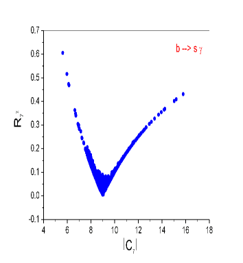
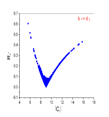
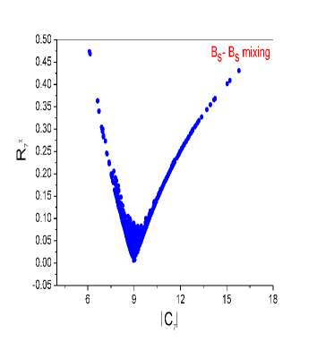
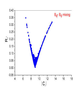
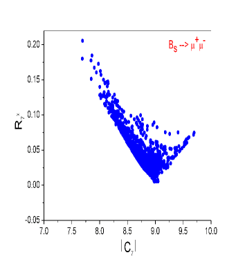
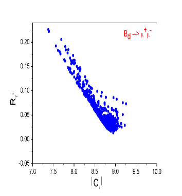
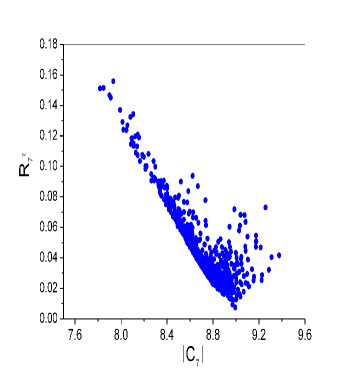
In order to estimate the enhancement in the full Wilson coefficients $C_{7}$ and $C_{9}$ due to chargino contribution we define the two ratios: $R^{\chi}_{7}=\frac{|C^{{\chi}}_{7}|}{|C_{7}|}$ and $R^{\chi}_{9}=\frac{|C^{{\chi}}_{9}|}{|C_{9}|}$ where $C_{7}$ and $C_{9}$ are the total Wilson coefficients. We start our numerical analysis by displaying the results of imposing the different constraints on the MSSM parameter space. For simplicity we only show the plots of $R^{\chi}_{7}$ versus $|C_{7}|$ for the points in the MSSM parameter space passing one constraint per time. Moreover, we show the corresponding constraints in the $b\to s$ and $b\to d$ transitions. This will help us to compare the strength of the corresponding constraints in the two sectors. In Fig.(1) we plot $R^{\chi}_{7}$ verses $|C_{7}|$ for the points allowed by $b\to s\gamma$ and $b\to d\gamma$ constraints. The left diagram corresponds to the points passing $b\to s\gamma$ constraint and the right one corresponds to the points passing $b\to d\gamma$ constraint. For the points with $C^{{\chi}}_{7}$ is much smaller than $C^{SM}_{7}$ we expect that $R^{\chi}_{7}$ to be close to zero and $|C_{7}|$ to be close to $|C^{SM}_{7}|\simeq 9\times 10^{-5}$ which is clear from the kink in Fig.(1). On the other hand the points in the parameter space that lead to sign $C^{{\chi}}_{7}$ similar(opposite) to sign $C^{SM}_{7}$ will enhance(reduce) $|C_{7}|$ which in turn reduces(enhances)$R^{\chi}_{7}$ which can be seen in the Figure. We see also from Fig.(1) that the maximum value of $R^{\chi}_{7}$ is about 0.6 which means that $C_{7}$ can be enhanced by about 60% for all points passing both constraints. Clearly this indicates that these constraints are not the strongest ones as we will see below. Next we consider the constraints from $B_{q}-B_{q}$ mixing where as before q=d,sπ‘žπ‘‘π‘ q=d,s. We plot the corresponding graphs in Fig.(2). The plots in that figure have several features like the plots in Fig.(1). The differences between the two figures are that $C_{7}$ can be enhanced by about 45% and 35% for the points passing $B_{s}-B_{s}$ and $B_{d}-B_{d}$ mixing constraints respectively. This implies that the constraints from $B_{q}-B_{q}$ mixing are stronger than those from $b\to s\gamma$ and $b\to d\gamma$ constraints. Moreover, the constraint from $B_{d}-B_{d}$ is stronger than that of $B_{s}-B_{s}$ mixing constraint. In Fig.(3) we display the points passing the $B_{q}\to\mu^{+}\mu^{-}$ constraints where q=d,sπ‘žπ‘‘π‘ q=d,s. As can be seen from Fig.(3), $C_{7}$ can be enhanced by less than 20% in both plots. Clearly $B_{q}\to\mu^{+}\mu^{-}$ provides the strongest constraints in both $b\to s$ and $b\to d$ transitions. We notice also from Fig.(3) that the constraint from $B_{d}\to\mu^{+}\mu^{-}$ are slightly stronger than that of $B_{s}\to\mu^{+}\mu^{-}$ which is clear from the maximum value that $|C_{7}|$ can reach where we find that $|C_{7}|$ can reach $9.25\times 10^{-5}$ and $9.75\times 10^{-5}$ after considering $B_{d}\to\mu^{+}\mu^{-}$ and $B_{s}\to\mu^{+}\mu^{-}$ respectively.

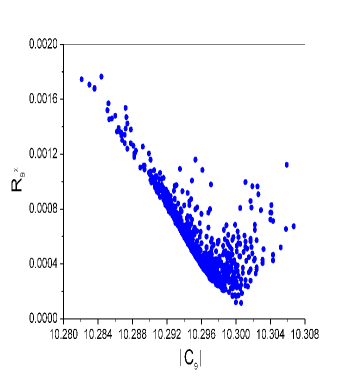
We now apply all constraints on the MSSM parameter space at the same time and present our predictions for the ratios $R^{\chi}_{7,9}$ and the branching ratios (BR) of $(\bar{B}_{s}\to\phi\pi^{0})$ and $(\bar{B}_{s}\to\phi\rho^{0})$. In Fig.(4) we plot $R^{\chi}_{7}$ verses $|C_{7}|$ and $R^{\chi}_{9}$ versus $|C_{9}|$ for the allowed points in the parameter space. The left diagram corresponds to $R^{\chi}_{7}$ versus $|C_{7}|$ in units of $10^{-5}$ while the right diagram corresponds to $R^{\chi}_{9}$ versus $|C_{9}|$ in units of $10^{-3}$. As can be seen from Fig.(4) that, $C_{7}$ can be enhanced by less than 20 % and $C_{9}$ can be enhanced by less than 1 %. In order to explain this result we note that the dominant contributions to $C^{\tilde{\chi}}_{7}$ and $C^{\tilde{\chi}}_{9}$ come from Z penguins which are expressed in terms of $Y_{1Z}$ and $Y_{2Z}$ respectively as given in the Appendix. The ratio $\mid Y_{2Z}/Y_{1Z}\mid\simeq 1.2$ which means that the full Wilson coefficients $C_{7}$ and $C_{9}$ will be enhanced by the same order of magnitude and since $C^{SM}_{9}\gg C^{SM}_{7}$ we can expect that $R^{\chi}_{9}\ll R^{\chi}_{7}$ which is the same result that we obtained in Fig.(4). As a consequence we expect that SUSY contributions will not enhance the branching ratios of $(\bar{B}_{s}\to\phi\pi^{0})$ and $(\bar{B}_{s}\to\phi\rho^{0})$ sizeably.

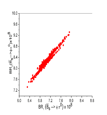
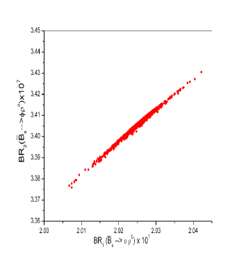
In Fig.(5) we plot the branching ratios of $(\bar{B}_{s}\to\phi\pi^{0})$ and $(\bar{B}_{s}\to\phi\rho^{0})$ resulting after the scan over the MSSM parameter space subjected to the constraints discussed above. The left diagram corresponds to BR $(\bar{B}_{s}\to\phi\pi^{0})$ while the right diagram corresponds to BR $(\bar{B}_{s}\to\phi\rho^{0})$. In both diagrams we present the predictions corresponding to solution $1$ and $2$ of the SCET parameters. Clearly from Fig.(5) SUSY contributions can enhance BR $(\bar{B}_{s}\to\phi\pi^{0})$ by about 14% and 3% with respect to the SM prediction for solution 1 and 2 of the SCET parameters respectively. For BR $(\bar{B}_{s}\to\phi\rho^{0})$, we see from Fig.(5) that SUSY contributions enhance the branching ratios by about 1% with respect to the SM prediction for both solution 1 and 2 of the SCET parameters. The reason for the significant enhancement of the branching ratios in case of $(\bar{B}_{s}\to\phi\pi^{0})$ compared to the branching ratios of $(\bar{B}_{s}\to\phi\rho^{0})$ due to SUSY contributions can be attributed to the difference in the sign of $C_{7}$ in their amplitudes given in eqs.(13,16) and eqs.(14,17) for solution 1 and 2 of the SCET parameters respectively. Thus an enhancement of $C_{7}$ will lead to opposite effects in the total amplitudes of $(\bar{B}_{s}\to\phi\pi^{0})$ and $(\bar{B}_{s}\to\phi\rho^{0})$ and thus in their branching ratios as we obtained in Fig.(5).

We end this section by comparing our results with the results given in ref.Hofer:2010ee . We find that no sizeable enhancement of the EW penguins Wilson coefficients in the MSSM with flavour-violation in the up sector that may lead to large effects in the decays $\bar{B}_{s}\to\phi\pi^{0}$ and $\bar{B}_{s}\to\phi\rho^{0}$ in agreement with the conclusion of ref.Hofer:2010ee .

Refer to caption
Refer to caption
Figure 5: Branching ratios of $(\bar{B}_{s}\to\phi\pi^{0})$ and $(\bar{B}_{s}\to\phi\rho^{0})$. Left plot corresponds to BR $(\bar{B}_{s}\to\phi\pi^{0})\times 10^{8}$ while right plot corresponds to BR $(\bar{B}_{s}\to\phi\rho^{0})\times 10^{8}$. In the Figure $BR_{1}$ and $BR_{2}$ refer to the branching ratios correspond to predictions 1 and 2 in Table 1.

V Conclusion

In this article we have studied the decay modes $\bar{B}_{s}\to\phi\pi^{0}$ and $\bar{B}_{s}\to\phi\rho^{0}$ using SCET. Within SM, we find that BR $\bar{B}_{s}\to\phi\pi^{0}=7_{-1-2}^{+1+2}\times 10^{-8}$ and BR $\bar{B}_{s}\to\phi\pi^{0}=9_{-1-4}^{+1+3}\times 10^{-8}$ corresponding to solution $1$ and solution $2$ of the SCET parameters respectively. In addition we find that BR $\bar{B}_{s}\to\phi\rho^{0}=20.2^{+1+9}_{-1-12}\times 10^{-8}$ and BR $\bar{B}_{s}\to\phi\rho^{0}=34.0^{+1.5+15}_{-1.5-22}\times 10^{-8}$ corresponding to solution $1$ and solution $2$ of the SCET parameters respectively. Clearly, within SM, the decay modes $\bar{B}_{s}\to\phi\pi^{0}$ and $\bar{B}_{s}\to\phi\rho^{0}$ have tiny branching ratios of order $\sim 10^{-7}$ leading to a difficulty in observing them. As a consequence any significant enhancement of their branching ratios making them observable at LHC will be a clear indication of New Physics beyond SM.

We have analyzed SUSY contributions to the branching ratios of $(\bar{B}_{s}\to\phi\pi^{0})$ and $(\bar{B}_{s}\to\phi\rho^{0})$ decays using SCET. We have adopted in our analysis exact diagonalization of the squark mass matrices. We have shown that, BR $(\bar{B}_{s}\to\phi\pi^{0})$ can be enhanced by about 14% and 3% with respect to the SM predictions for solution 1 and 2 of the SCET parameters respectively. For BR $(\bar{B}_{s}\to\phi\rho^{0})$, we find that BR $(\bar{B}_{s}\to\phi\rho^{0})$ is enhanced by about 1% with respect to the SM predictions for both solution 1 and 2 of the SCET parameters. Clearly, SUSY contributions obtained from gluino and chargino mediation can not lead to a significant enhancement of the branching ratios of $(\bar{B}_{s}\to\phi\pi^{0})$ and $(\bar{B}_{s}\to\phi\rho^{0})$ decays making them easily detectable at LHC. Moreover, in case of observation of these decays due to improved experimental techniques it will not be possible to pin down the SUSY contributions.

Acknowledgement

Gaber Faisel’s work is supported by the National Science Council of R.O.C. under grants NSC 99-2112-M-008-003-MY3 and NSC 100-2811-M-008-036.

Appendix A Appendix

The chargino contributions to the Wilson coefficients are given byDu:1997zc ; Kruger:2000ff

$\displaystyle C_{1}^{{\chi}}$ $\displaystyle=$ $\displaystyle 0,$
$\displaystyle C_{2}^{{\chi}}$ $\displaystyle=$ $\displaystyle 0,$
$\displaystyle C_{3}^{{\chi}}$ $\displaystyle=$ $\displaystyle-\frac{\alpha_{s}}{24\pi}Z,$
$\displaystyle C_{4}^{{\chi}}$ $\displaystyle=$ $\displaystyle\frac{\alpha_{s}}{8\pi}Z,$
$\displaystyle C_{5}^{{\chi}}$ $\displaystyle=$ $\displaystyle-\frac{\alpha_{s}}{24\pi}Z,$
$\displaystyle C_{6}^{{\chi}}$ $\displaystyle=$ $\displaystyle\frac{\alpha_{s}}{8\pi}Z,$
$\displaystyle C_{7}^{{\chi}}$ $\displaystyle=$ $\displaystyle\frac{\alpha}{6\pi}Y_{1},$
$\displaystyle C_{8}^{{\chi}}$ $\displaystyle=$ $\displaystyle 0,$
$\displaystyle C_{9}^{{\chi}}$ $\displaystyle=$ $\displaystyle\frac{\alpha}{6\pi}Y_{2},$
$\displaystyle C_{10}^{{\chi}}$ $\displaystyle=$ $\displaystyle 0.$
$\displaystyle C_{7\gamma}^{{\chi}}$ $\displaystyle=$ βˆ’16​g2β€‹βˆ‘A=16βˆ‘j=12MW2mΟ‡j~Β±2​[(XjUL⁣†)2​A​(XjUL)A​3​f1​(mu~A2mΟ‡~jΒ±2)βˆ’2​(XjUL⁣†)2​A​(XjUR)A​3​mΟ‡j~Β±mb​f2​(mu~A2mΟ‡~jΒ±2)],16superscript𝑔2superscriptsubscript𝐴16superscriptsubscript𝑗12superscriptsubscriptπ‘€π‘Š2subscriptsuperscriptπ‘š2superscript~subscriptπœ’π‘—plus-or-minusdelimited-[]subscriptsuperscriptsubscript𝑋𝑗subscriptπ‘ˆπΏβ€ 2𝐴subscriptsuperscriptsubscript𝑋𝑗subscriptπ‘ˆπΏπ΄3subscript𝑓1subscriptsuperscriptπ‘š2subscript~𝑒𝐴subscriptsuperscriptπ‘š2superscriptsubscript~πœ’π‘—plus-or-minus2subscriptsuperscriptsubscript𝑋𝑗subscriptπ‘ˆπΏβ€ 2𝐴subscriptsuperscriptsubscript𝑋𝑗subscriptπ‘ˆπ‘…π΄3subscriptπ‘šsuperscript~subscriptπœ’π‘—plus-or-minussubscriptπ‘šπ‘subscript𝑓2subscriptsuperscriptπ‘š2subscript~𝑒𝐴subscriptsuperscriptπ‘š2superscriptsubscript~πœ’π‘—plus-or-minus\displaystyle-\frac{1}{6g^{2}}\sum_{A=1}^{6}\sum_{j=1}^{2}\frac{M_{W}^{2}}{m^{2}_{\tilde{\chi_{j}}^{\pm}}}\Bigg{[}(X_{j}^{U_{L}\dagger})_{2A}(X_{j}^{U_{L}})_{A3}f_{1}(\frac{m^{2}_{\tilde{u}_{A}}}{m^{2}_{\tilde{\chi}_{j}^{\pm}}})-2(X_{j}^{U_{L}\dagger})_{2A}(X_{j}^{U_{R}})_{A3}\frac{m_{\tilde{\chi_{j}}^{\pm}}}{m_{b}}f_{2}(\frac{m^{2}_{\tilde{u}_{A}}}{m^{2}_{\tilde{\chi}_{j}^{\pm}}})\Bigg{]},
$\displaystyle C_{8g}^{{\chi}}$ $\displaystyle=$ βˆ’16​g2β€‹βˆ‘A=16βˆ‘j=12MW2mΟ‡j~Β±2​[(XjUL⁣†)2​A​(XjUL)A​3​g1​(mu~A2mΟ‡~jΒ±2)βˆ’2​(XjUL⁣†)2​A​(XjUR)A​3​mΟ‡j~Β±2mb​g2​(mu~A2mΟ‡~jΒ±2)]16superscript𝑔2superscriptsubscript𝐴16superscriptsubscript𝑗12superscriptsubscriptπ‘€π‘Š2subscriptsuperscriptπ‘š2superscript~subscriptπœ’π‘—plus-or-minusdelimited-[]subscriptsuperscriptsubscript𝑋𝑗subscriptπ‘ˆπΏβ€ 2𝐴subscriptsuperscriptsubscript𝑋𝑗subscriptπ‘ˆπΏπ΄3subscript𝑔1subscriptsuperscriptπ‘š2subscript~𝑒𝐴subscriptsuperscriptπ‘š2superscriptsubscript~πœ’π‘—plus-or-minus2subscriptsuperscriptsubscript𝑋𝑗subscriptπ‘ˆπΏβ€ 2𝐴subscriptsuperscriptsubscript𝑋𝑗subscriptπ‘ˆπ‘…π΄3subscriptsuperscriptπ‘š2superscript~subscriptπœ’π‘—plus-or-minussubscriptπ‘šπ‘subscript𝑔2subscriptsuperscriptπ‘š2subscript~𝑒𝐴subscriptsuperscriptπ‘š2superscriptsubscript~πœ’π‘—plus-or-minus\displaystyle-\frac{1}{6g^{2}}\sum_{A=1}^{6}\sum_{j=1}^{2}\frac{M_{W}^{2}}{m^{2}_{\tilde{\chi_{j}}^{\pm}}}\Bigg{[}(X_{j}^{U_{L}\dagger})_{2A}(X_{j}^{U_{L}})_{A3}g_{1}(\frac{m^{2}_{\tilde{u}_{A}}}{m^{2}_{\tilde{\chi}_{j}^{\pm}}})-2(X_{j}^{U_{L}\dagger})_{2A}(X_{j}^{U_{R}})_{A3}\frac{m^{2}_{\tilde{\chi_{j}}^{\pm}}}{m_{b}}g_{2}(\frac{m^{2}_{\tilde{u}_{A}}}{m^{2}_{\tilde{\chi}_{j}^{\pm}}})\Bigg{]} (44)

We can write $Y_{i}=Y_{iZ}+Y_{i\gamma}$ for $i=1,2$ where $Y_{iZ}$ refers to the contribution from chargino loops with a Z-boson coupling to the quark pair , $Y_{i\gamma}$ refers to contribution from chargino loops with a photon coupling to the quark pair and Z refers to contribution from chargino loops with a gluon coupling to the quark pair. Their explicit expressions are given as

$\displaystyle Z$ $\displaystyle=$ $\displaystyle-\displaystyle\frac{1}{3g^{2}_{2}V^{*}_{ts}V_{tb}}\displaystyle\sum_{A=1}^{6}\displaystyle\sum_{i=1}^{2}\displaystyle\frac{m^{2}_{W}}{m^{2}_{\tilde{u}_{A}}}(X_{i}^{U_{L}})_{2A}^{+}(X_{i}^{U_{L}})_{A3}f_{5}\left(\displaystyle\frac{m^{2}_{\tilde{\chi}_{i}^{\pm}}}{m^{2}_{\tilde{u}_{A}}}\right),$
$\displaystyle Y_{1Z}$ $\displaystyle=$ $\displaystyle-\displaystyle\frac{2}{g^{2}_{2}V^{*}_{ts}V_{tb}}\displaystyle\sum_{A,B=1}^{6}\displaystyle\sum_{i,j=1}^{2}(X_{i}^{U_{L}})_{2A}^{+}(X_{j}^{U_{L}})_{B3}\left\{c_{2}(m^{2}_{\tilde{\chi}_{i}^{\pm}},m^{2}_{\tilde{u}_{A}},m^{2}_{\tilde{u}_{B}})(\Gamma^{U_{L}}\Gamma^{U_{L}+})_{AB}\delta_{ij}\right.$
$\displaystyle-c_{2}(m^{2}_{\tilde{u}_{A}},m^{2}_{\tilde{\chi}_{i}^{\pm}},m^{2}_{\tilde{\chi}_{j}^{\pm}})\delta_{AB}V_{i1}^{*}V_{j1}+\displaystyle\frac{1}{2}m_{\tilde{\chi}_{i}^{\pm}}m_{\tilde{\chi}_{j}^{\pm}}c_{0}(m^{2}_{\tilde{u}_{A}},m^{2}_{\tilde{\chi}_{i}^{\pm}},m^{2}_{\tilde{\chi}_{j}^{\pm}})\delta_{AB}U_{i1}U_{j1}^{*}\left.\right\},$
$\displaystyle Y_{2Z}$ $\displaystyle=$ $\displaystyle\left(\displaystyle\frac{1}{sin^{2}\theta_{w}}-2\right)\displaystyle\frac{1}{g^{2}_{2}V^{*}_{ts}V_{tb}}\displaystyle\sum_{A,B=1}^{6}\displaystyle\sum_{i,j=1}^{2}(X_{i}^{U_{L}})_{2A}^{+}(X_{j}^{U_{L}})_{B3}\left\{c_{2}(m^{2}_{\tilde{\chi}_{i}^{\pm}},m^{2}_{\tilde{u}_{A}},m^{2}_{\tilde{u}_{B}})(\Gamma^{U_{L}}\Gamma^{U_{L}+})_{AB}\delta_{ij}\right.$
$\displaystyle-c_{2}(m^{2}_{\tilde{u}_{A}},m^{2}_{\tilde{\chi}_{i}^{\pm}},m^{2}_{\tilde{\chi}_{j}^{\pm}})\delta_{AB}V_{i1}^{*}V_{j1}+\displaystyle\frac{1}{2}m_{\tilde{\chi}_{i}^{\pm}}m_{\tilde{\chi}_{j}^{\pm}}c_{0}(m^{2}_{\tilde{u}_{A}},m^{2}_{\tilde{\chi}_{i}^{\pm}},m^{2}_{\tilde{\chi}_{j}^{\pm}})\delta_{AB}U_{i1}U_{j1}^{*}\left.\right\},$
$\displaystyle Y_{1\gamma}$ $\displaystyle=$ $\displaystyle Y_{2\gamma}=-\displaystyle\frac{1}{9g^{2}_{2}V^{*}_{ts}V_{tb}}\displaystyle\sum_{A=1}^{6}\displaystyle\sum_{i=1}^{2}\displaystyle\frac{m^{2}_{W}}{m^{2}_{\tilde{u}_{A}}}(X_{i}^{U_{L}})_{2A}^{+}(X_{i}^{U_{L}})_{A3}f_{4}\left(\displaystyle\frac{m^{2}_{\tilde{\chi}_{i}^{\pm}}}{m^{2}_{\tilde{u}_{A}}}\right).$ (45)

where

$\displaystyle X_{i}^{UL}$ $\displaystyle=$ $\displaystyle g\bigg{[}-V^{*}_{i1}\Gamma^{UL}+V^{*}_{i2}\Gamma^{UR}\frac{M_{U}}{\sqrt{2}m_{W}\sin\beta}\bigg{]}K$
$\displaystyle X_{i}^{UR}$ $\displaystyle=$ $\displaystyle g\bigg{[}U_{i2}\Gamma^{UL}K\frac{M_{D}}{\sqrt{2}m_{W}\cos\beta}\bigg{]}$ (46)

and the loop functions are given as follows

$\displaystyle g_{1}(x)$ $\displaystyle=$ $\displaystyle\frac{-6-15x+3x^{2}}{6(1-x)^{3}}+\frac{-3xlnx}{(1-x)^{4}}$
$\displaystyle g_{2}(x)$ $\displaystyle=$ $\displaystyle\frac{3x+3}{2(1-x)^{2}}+\frac{3xlnx}{(1-x)^{3}}-\frac{3}{2},$
$\displaystyle f_{1}(x)$ $\displaystyle=$ $\displaystyle\frac{-7+5x+8x^{2}}{6(1-x)^{3}}-\frac{x(2-3x)lnx}{(1-x)^{4}},$
$\displaystyle f_{2}(x)$ $\displaystyle=$ $\displaystyle\frac{x(3-5x)}{2(1-x)^{2}}+\frac{x((2-3x)lnx)}{(1-x)^{3}},$
$\displaystyle f_{4}(x)$ $\displaystyle=$ $\displaystyle\displaystyle\frac{52-101x+43x^{2}}{6(1-x)^{3}}+\displaystyle\frac{6-9x+2x^{3}}{(1-x)^{4}}lnx,$
$\displaystyle f_{5}(x)$ $\displaystyle=$ $\displaystyle\displaystyle\frac{2-7x+11x^{2}}{6(1-x)^{3}}+\displaystyle\frac{x^{3}}{(1-x)^{4}}lnx,$
$\displaystyle c_{0}(m_{1}^{2},m_{2}^{2},m_{3}^{2})$ $\displaystyle=$ $\displaystyle-\left(\displaystyle\frac{m_{1}^{2}ln(m_{1}^{2}/\mu^{2})}{(m_{1}^{2}-m_{2}^{2})(m_{1}^{2}-m_{3}^{2})}+(m_{1}\leftrightarrow m_{2})+(m_{1}\leftrightarrow m_{3})\right),$
$\displaystyle c_{2}(m_{1}^{2},m_{2}^{2},m_{3}^{2})$ $\displaystyle=$ $\displaystyle\displaystyle\frac{3}{8}-\displaystyle\frac{1}{4}\left(\displaystyle\frac{m_{1}^{4}ln(m_{1}^{2}/\mu^{2})}{(m_{1}^{2}-m_{2}^{2})(m_{1}^{2}-m_{3}^{2})}+(m_{1}\leftrightarrow m_{2})+(m_{1}\leftrightarrow m_{3})\right).$ (47)

The gluino contributions to the Wilson coefficients are given byHarnik:2002vs

$\displaystyle C_{1}^{\tilde{g}}$ $\displaystyle=$ $\displaystyle 0,$
$\displaystyle C_{2}^{\tilde{g}}$ $\displaystyle=$ $\displaystyle 0,$
$\displaystyle C^{\tilde{g}}_{3}$ $\displaystyle=$ $\displaystyle\frac{\alpha_{s}^{2}\sqrt{2}}{m_{\tilde{g}}^{2}G_{F}}\left(\sum_{AB}\Gamma^{L\ast}_{sA}\Gamma^{L}_{bA}\Gamma^{L\ast}_{sB}\Gamma^{L}_{sB}\left[-\frac{1}{9}B_{1}(x_{A},x_{B})-\frac{5}{9}B_{2}(x_{A},x_{B})\right]\right.$
$\displaystyle\ \ \ \ \ \ \ \left.+\sum_{A}\Gamma^{R\ast}_{sA}\Gamma^{R}_{bA}\left[-\frac{1}{18}C_{1}(x_{A})+\frac{1}{2}C_{2}(x_{A})\right]\right)$
$\displaystyle C^{\tilde{g}}_{4}$ $\displaystyle=$ $\displaystyle\frac{\alpha_{s}^{2}\sqrt{2}}{m_{\tilde{g}}^{2}G_{F}}\left(\sum_{AB}\Gamma^{L\ast}_{sA}\Gamma^{L}_{bA}\Gamma^{L\ast}_{sB}\Gamma^{L}_{sB}\left[-\frac{7}{3}B_{1}(x_{A},x_{B})+\frac{1}{3}B_{2}(x_{A},x_{B})\right]\right.$
$\displaystyle\ \ \ \ \ \ \ \left.+\sum_{A}\Gamma^{L\ast}_{sA}\Gamma^{L}_{bA}\left[\frac{1}{6}C_{1}(x_{A})-\frac{3}{2}C_{2}(x_{A})\right]\right)$
$\displaystyle C^{\tilde{g}}_{5}$ $\displaystyle=$ $\displaystyle\frac{\alpha_{s}^{2}\sqrt{2}}{m_{\tilde{g}}^{2}G_{F}}\left(\sum_{AB}\Gamma^{L\ast}_{sA}\Gamma^{L}_{bA}\Gamma^{R\ast}_{sB}\Gamma^{R}_{sB}\left[\frac{10}{9}B_{1}(x_{A},x_{B})+\frac{1}{18}B_{2}(x_{A},x_{B})\right]\right.$
$\displaystyle\ \ \ \ \ \ \ \left.+\sum_{A}\Gamma^{L\ast}_{sA}\Gamma^{L}_{bA}\left[-\frac{1}{18}C_{1}(x_{A})+\frac{1}{2}C_{2}(x_{A})\right]\right)$
$\displaystyle C^{\tilde{g}}_{6}$ $\displaystyle=$ $\displaystyle\frac{\alpha_{s}^{2}\sqrt{2}}{m_{\tilde{g}}^{2}G_{F}}\left(\sum_{AB}\Gamma^{L\ast}_{sA}\Gamma^{L}_{bA}\Gamma^{R\ast}_{sB}\Gamma^{R}_{sB}\left[-\frac{2}{3}B_{1}(x_{A},x_{B})+\frac{7}{6}B_{2}(x_{A},x_{B})\right]\right.$
$\displaystyle\ \ \ \ \ \ \ \left.+\sum_{A}\Gamma^{L\ast}_{sA}\Gamma^{L}_{bA}\left[\frac{1}{6}C_{1}(x_{A})-\frac{3}{2}C_{2}(x_{A})\right]\right)$
$\displaystyle C^{\tilde{g}}_{7\gamma}$ $\displaystyle=$ Ξ±s​π​2mg~2​GF​(βˆ‘AΞ“s​ALβ£βˆ—β€‹Ξ“b​AL​[βˆ’49​D1​(xA)]+mg~mbβ€‹βˆ‘AΞ“s​ALβ£βˆ—β€‹Ξ“b​AR​[βˆ’49​D2​(xA)])subscriptπ›Όπ‘ πœ‹2superscriptsubscriptπ‘š~𝑔2subscript𝐺𝐹subscript𝐴subscriptsuperscriptΞ“πΏβˆ—π‘ π΄subscriptsuperscriptΓ𝐿𝑏𝐴delimited-[]49subscript𝐷1subscriptπ‘₯𝐴subscriptπ‘š~𝑔subscriptπ‘šπ‘subscript𝐴subscriptsuperscriptΞ“πΏβˆ—π‘ π΄subscriptsuperscriptΓ𝑅𝑏𝐴delimited-[]49subscript𝐷2subscriptπ‘₯𝐴\displaystyle\frac{\alpha_{s}\pi\sqrt{2}}{m_{\tilde{g}}^{2}G_{F}}\left(\sum_{A}\Gamma^{L\ast}_{sA}\Gamma^{L}_{bA}\left[-\frac{4}{9}D_{1}(x_{A})\right]+\frac{m_{\tilde{g}}}{m_{b}}\sum_{A}\Gamma^{L\ast}_{sA}\Gamma^{R}_{bA}\left[-\frac{4}{9}D_{2}(x_{A})\right]\right)
$\displaystyle C^{\tilde{g}}_{8g}$ $\displaystyle=$ $\displaystyle\frac{\alpha_{s}\pi\sqrt{2}}{m_{\tilde{g}}^{2}G_{F}}\left(\sum_{A}\Gamma^{L\ast}_{sA}\Gamma^{L}_{bA}\left[-\frac{1}{6}D_{1}(x_{A})+\frac{3}{2}D_{3}(x_{A})\right]\right.$ (48)
$\displaystyle\ \ \ \ \ \ \ \left.+\frac{m_{\tilde{g}}}{m_{b}}\sum_{A}\Gamma^{L\ast}_{sA}\Gamma^{R}_{bA}\left[-\frac{1}{6}D_{2}(x_{A})+\frac{3}{2}D_{4}(x_{A})\right]\right).$

where $x_{A}\equiv m_{\tilde{d}_{A}}^{2}/m_{\tilde{g}}^{2}$ and the loop functions are given by

$\displaystyle B_{1}(x_{A},x_{B})$ $\displaystyle=$ $\displaystyle-\frac{x_{A}^{2}\log x_{A}}{4(x_{A}-x_{B})(x_{A}-1)^{2}}-\frac{x_{B}^{2}\log x_{B}}{4(x_{B}-x_{A})(x_{B}-1)^{2}}-\frac{1}{4(x_{A}-1)(x_{B}-1)},$
$\displaystyle B_{2}(x_{A},x_{B})$ $\displaystyle=$ $\displaystyle-\frac{x_{A}\log x_{A}}{(x_{A}-x_{B})(x_{A}-1)^{2}}-\frac{x_{B}\log x_{B}}{(x_{B}-x_{A})(x_{B}-1)^{2}}-\frac{1}{(x_{A}-1)(x_{B}-1)},$
$\displaystyle C_{1}(x)$ $\displaystyle=$ $\displaystyle\frac{2x^{3}-9x^{2}+18x-11-6\log x}{36(1-x)^{4}},$
$\displaystyle C_{2}(x)$ $\displaystyle=$ $\displaystyle\frac{-16x^{3}+45x^{2}-36x+7+6x^{2}(2x-3)\log x}{36(1-x)^{4}},$
$\displaystyle D_{1}(x)$ $\displaystyle=$ $\displaystyle\frac{-x^{3}+6x^{2}-3x-2-6x\log x}{6(1-x)^{4}},$
$\displaystyle D_{2}(x)$ $\displaystyle=$ $\displaystyle\frac{-x^{2}+1+2x\log x}{(x-1)^{3}},$
$\displaystyle D_{3}(x)$ $\displaystyle=$ $\displaystyle\frac{2x^{3}+3x^{2}-6x+1-6x^{2}\log x}{6(1-x)^{4}},$
$\displaystyle D_{4}(x)$ $\displaystyle=$ $\displaystyle\frac{-3x^{2}+4x-1+2x^{2}\log x}{(x-1)^{3}}.$ (49)

The Wilson coefficients $C^{\tilde{g}}_{i}$ for $i=7,...,10$ are given by Du:1997zc

$\displaystyle C_{7}^{\tilde{g}}$ $\displaystyle=$ $\displaystyle\frac{\alpha}{6\pi}Y_{1},$
$\displaystyle C_{8}^{\tilde{g}}$ $\displaystyle=$ $\displaystyle 0,$
$\displaystyle C_{9}^{\tilde{g}}$ $\displaystyle=$ $\displaystyle\frac{\alpha}{6\pi}Y_{2},$
$\displaystyle C_{10}^{\tilde{g}}$ $\displaystyle=$ $\displaystyle 0.$

where as before we write $Y_{i}=Y_{iZ}+Y_{i\gamma}$ for $i=1,2$ where $Y_{iZ}$ refers to the contribution from gluino loops with a Z-boson coupling to the quark pair, $Y_{i\gamma}$ refers to contribution from gluino loops with a photon coupling to the quark pair.

$\displaystyle Y_{1Z}$ $\displaystyle=$ $\displaystyle-\displaystyle\frac{16g^{2}_{3}}{3g^{2}_{2}V^{*}_{ts}V_{tb}}\displaystyle\sum_{A,B=1}^{6}(\Gamma^{D_{L}})^{\dagger}_{2A}(\Gamma^{D_{L}})_{B3}c_{2}(m^{2}_{\tilde{g}},m^{2}_{\tilde{d}_{A}},m^{2}_{\tilde{d}_{B}})(\Gamma^{D_{R}}\Gamma^{D_{R}{\dagger}})_{AB},$
$\displaystyle Y_{2Z}$ $\displaystyle=$ $\displaystyle\displaystyle\frac{8g^{2}_{3}}{3g^{2}_{2}V^{*}_{ts}V_{tb}}(\frac{1}{\sin^{2}\theta_{w}}-2)\displaystyle\sum_{A,B=1}^{6}(\Gamma^{D_{L}})^{\dagger}_{2A}(\Gamma^{D_{L}})_{B3}c_{2}(m^{2}_{\tilde{g}},m^{2}_{\tilde{d}_{A}},m^{2}_{\tilde{d}_{B}})(\Gamma^{D_{R}}\Gamma^{D_{R}{\dagger}})_{AB}$ (51)

and

$\displaystyle Y_{1\gamma}=Y_{2\gamma}$ $\displaystyle=$ $\displaystyle\displaystyle\frac{4g^{2}_{3}}{81g^{2}_{2}V^{*}_{ts}V_{tb}}\displaystyle\sum_{A=1}^{6}\displaystyle\frac{m^{2}_{W}}{m^{2}_{\tilde{d}_{A}}}(\Gamma^{D_{L}})^{\dagger}_{2A}(\Gamma^{D_{L}})_{A3}f_{6}\left(\displaystyle\frac{m^{2}_{\tilde{g}}}{m^{2}_{\tilde{d}_{A}}}\right),$

where

$\displaystyle f_{6}(x)$ $\displaystyle=$ $\displaystyle\displaystyle\frac{2-7x+11x^{2}}{(1-x)^{3}}+\displaystyle\frac{6x^{3}}{(1-x)^{4}}lnx,$

It should be noted that the expressions for $Y_{i}$ given in the last two equations are consistent with the corresponding expressions given in ref.Cho:1996we after replacing the lepton charge with the up quark charge and taking into account the effective Hamiltonian conventions used in ref.Cho:1996we . We further correct $Y_{1\gamma}$ and $Y_{2\gamma}$ given in equation B10 in ref.Du:1997zc . We also neglect the small contributions from the box diagrams to $C_{9}$ as the dominant contributions is due to Z penguinsHofer:2010ee .

References

  • (1) A. J. Buras, R. Fleischer, S. Recksiegel and F. Schwab, Phys. Rev. Lett. 92 (2004) 101804 [hep-ph/0312259]; Nucl. Phys. B 697 (2004) 133 [hep-ph/0402112].
  • (2) L. Hofer, D. Scherer and L. Vernazza, JHEP 1102, 080 (2011) [arXiv:1011.6319 [hep-ph]].
  • (3) F. Gabbiani, E. Gabrielli, A. Masiero and L. Silvestrini, Nucl. Phys.  B 477, 321 (1996) [arXiv:hep-ph/9604387].
  • (4) S. Khalil, A. Masiero and H. Murayama, Phys. Lett.  B 682, 74 (2009) [arXiv:0908.3216 [hep-ph]].
  • (5) A. Datta and S. Khalil, Phys. Rev.  D 80, 075006 (2009) [arXiv:0905.2105 [hep-ph]].
  • (6) S. Khalil, Eur. Phys. J.  C 50, 35 (2007) [arXiv:hep-ph/0604118].
  • (7) S. Khalil and O. Lebedev, Phys. Lett.  B 515, 387 (2001) [arXiv:hep-ph/0106023].
  • (8) G. Faisel, D. Delepine and M. Shalaby, Phys. Lett. B 705, 361 (2011) [arXiv:1101.2710 [hep-ph]].
  • (9) S. Khalil, JHEP 0212, 012 (2002) [arXiv:hep-ph/0202204].
  • (10) D. Delepine, G. Faisel, S. Khalil and M. Shalaby, Int. J. Mod. Phys.  A 22, 6011 (2007).
  • (11) D. Delepine, G. Faisel and S. Khalil, Phys. Rev.  D 77, 016003 (2008) [arXiv:0710.1441 [hep-ph]].
  • (12) D. Delepine, G. Faisl, S. Khalil and G. L. Castro, Phys. Rev.  D 74, 056004 (2006) [arXiv:hep-ph/0608008].
  • (13) M. Beneke and M. Neubert, Nucl. Phys.  B 675, 333 (2003) [arXiv:hep-ph/0308039].
  • (14) A. Ali, G. Kramer, Y. Li, C. D. Lu, Y. L. Shen, W. Wang and Y. M. Wang, Phys. Rev.  D 76, 074018 (2007) [arXiv:hep-ph/0703162].
  • (15) C. W. Bauer, S. Fleming and M. E. Luke, Phys. Rev.  D 63, 014006 (2000) [arXiv:hep-ph/0005275].
  • (16) C. W. Bauer, S. Fleming, D. Pirjol and I. W. Stewart, Phys. Rev.  D 63, 114020 (2001) [arXiv:hep-ph/0011336].
  • (17) J. Chay and C. Kim, Phys. Rev. D 68, 071502 (2003) [arXiv:hep-ph/0301055]. Chay:2003ju
  • (18) J. Chay and C. Kim, Nucl. Phys. B 680, 302 (2004) [arXiv:hep-ph/0301262].
  • (19) W. Wang, Y. M. Wang, D. S. Yang and C. D. Lu, Phys. Rev.  D 78, 034011 (2008) [arXiv:0801.3123 [hep-ph]].
  • (20) L. Hofer, D. Scherer and L. Vernazza, arXiv:1104.5521 [hep-ph].
  • (21)
  • (22) S. Fleming, PoS E FT09, 002 (2009) [arXiv:0907.3897 [hep-ph]].
  • (23) A. Jain, I. Z. Rothstein and I. W. Stewart, arXiv:0706.3399 [hep-ph].
  • (24) C. W. Bauer, D. Pirjol and I. W. Stewart, Phys. Rev.  D 67, 071502 (2003) [arXiv:hep-ph/0211069].
  • (25) C. W. Bauer, I. Z. Rothstein and I. W. Stewart, Phys. Rev.  D 74, 034010 (2006) [arXiv:hep-ph/0510241].
  • (26) A. R. Williamson and J. Zupan, Phys. Rev.  D 74, 014003 (2006) [Erratum-ibid.  D 74, 03901 (2006)] [arXiv:hep-ph/0601214].
  • (27) C. W. Bauer, D. Pirjol, I. Z. Rothstein and I. W. Stewart, Phys. Rev. D 70, 054015 (2004) [arXiv:hep-ph/0401188].
  • (28) M. Beneke, G. Buchalla, M. Neubert and C. T. Sachrajda, Nucl. Phys.  B 591, 313 (2000) [arXiv:hep-ph/0006124].
  • (29) M. Beneke, G. Buchalla, M. Neubert and C. T. Sachrajda, Phys. Rev. Lett.  83, 1914 (1999) [arXiv:hep-ph/9905312].
  • (30) M. Beneke and S. Jager, Nucl. Phys.  B 751, 160 (2006) [arXiv:hep-ph/0512351].
  • (31) M. Beneke and S. Jager, Nucl. Phys.  B 768, 51 (2007) [arXiv:hep-ph/0610322].
  • (32) R. Fleischer, Phys. Lett. B 332, 419 (1994).
  • (33) G. Buchalla, A. J. Buras and M. E. Lautenbacher, Rev. Mod. Phys 68, 1230 (1996) [arXiv:hep-ph/9512380].
  • (34) J. G. Korner and G. R. Goldstein, Phys. Lett.  B 89, 105 (1979).
  • (35) P. L. Cho, M. Misiak and D. Wyler, Phys. Rev.  D 54, 3329 (1996) [arXiv:hep-ph/9601360].
  • (36) K. Huitu and S. Khalil, Phys. Rev.  D 81, 095008 (2010) [arXiv:0911.1868 [hep-ph]].
  • (37) A. Masiero and H. Murayama, Phys. Rev. Lett.  83, 907 (1999) [arXiv:hep-ph/9903363].
  • (38) S. A. Abel and J. M. Frere, Phys. Rev.  D 55, 1623 (1997) [arXiv:hep-ph/9608251].
  • (39) S. Khalil, T. Kobayashi and A. Masiero, Phys. Rev.  D 60, 075003 (1999) [arXiv:hep-ph/9903544].
  • (40) S. Khalil and T. Kobayashi,endthebibliography Phys. Lett.  B 460, 341 (1999) [arXiv:hep-ph/9906374].
  • (41) R. Barbieri, R. Contino and A. Strumia, Nucl. Phys.  B 578, 153 (2000) [arXiv:hep-ph/9908255].
  • (42) K. S. Babu, B. Dutta and R. N. Mohapatra, Phys. Rev.  D 61, 091701 (2000) [arXiv:hep-ph/9905464].
  • (43) M. Brhlik, L. L. Everett, G. L. Kane, S. F. King and O. Lebedev, Phys. Rev. Lett.  84, 3041 (2000) [arXiv:hep-ph/9909480].
  • (44) D. Bailin and S. Khalil, Phys. Rev. Lett.  86, 4227 (2001) [arXiv:hep-ph/0010058].
  • (45) S. Khalil, T. Kobayashi and O. Vives, Nucl. Phys.  B 580, 275 (2000) [arXiv:hep-ph/0003086].
  • (46) T. Kobayashi and O. Vives, Phys. Lett.  B 506, 323 (2001)
  • (47) L. L. Everett, G. L. Kane, S. Rigolin, L. T. Wang and T. T. Wang, JHEP 0201, 022 (2002) [arXiv:hep-ph/0112126].
  • (48) J. A. Casas, A. Lleyda and C. Munoz, Nucl. Phys.  B 471, 3 (1996) [arXiv:hep-ph/9507294].
  • (49) J. A. Casas and S. Dimopoulos, Phys. Lett.  B 387, 107 (1996) [arXiv:hep-ph/9606237].
  • (50) W. BuchmΓΌller and D. Wyler, Phys. Lett. B121 (1983) 321; J. Polchinski and M.B. Wise, Phys. Lett. B125 (1983) 393
  • (51) S. Bertolini, F. Borzumati, A. Masiero and G. Ridolfi, Nucl. Phys.  B 353, 591 (1991).
  • (52) ATLAS Collaboration Collaboration, G. Aad et al., Search for squarks and gluinos using final states with jets and missing transverse momentum with the ATLAS detector in sqrt(s) = 7 TeV proton-proton collisions, arXiv:1109.6572.
  • (53) S. Chatrchyan et al. [CMS Collaboration], arXiv:1109.2352 [hep-ex].
  • (54) J. Berger, M. Perelstein, M. Saelim and A. Spray, arXiv:1111.6594 [hep-ph].
  • (55) K. Nakamura et al. [ Particle Data Group Collaboration ], J. Phys. G G37, 075021 (2010).
  • (56) M. Ciuchini, G. Degrassi, P. Gambino and G. F. Giudice, Nucl. Phys.  B 534, 3 (1998) [arXiv:hep-ph/9806308].
  • (57) F. Borzumati, C. Greub and Y. Yamada, Phys. Rev.  D 69, 055005 (2004) [arXiv:hep-ph/0311151].
  • (58) G. Degrassi, P. Gambino and P. Slavich, Phys. Lett.  B 635, 335 (2006) [arXiv:hep-ph/0601135].
  • (59) G. Degrassi, P. Gambino and G. F. Giudice, JHEP 0012 (2000) 009 [arXiv:hep-ph/0009337].
  • (60) M. S. Carena, D. Garcia, U. Nierste and C. E. M. Wagner, Phys. Lett.  B 499 (2001) 141 [arXiv:hep-ph/0010003].
  • (61) G. D’Ambrosio, G. F. Giudice, G. Isidori and A. Strumia, Nucl. Phys.  B 645 (2002) 155 [arXiv:hep-ph/0207036].
  • (62) A. J. Buras, P. H. Chankowski, J. Rosiek and L. Slawianowska, Nucl. Phys.  B 659 (2003) 3 [arXiv:hep-ph/0210145].
  • (63) S. Bertolini, F. Borzumati and A. Masiero, Phys. Lett.  B 192, 437 (1987).
  • (64) C. Bobeth, M. Misiak and J. Urban, Nucl. Phys.  B 567 (2000) 153 [arXiv:hep-ph/9904413].
  • (65) E. Gabrielli, S. Khalil and E. Torrente-Lujan, Nucl. Phys. B 594, 3 (2001).
  • (66) A. L. Kagan and M. Neubert, Phys. Rev. D 58 094012 (1998).
  • (67) S. Khalil, Phys. Rev.  D72, 035007 (2005). [hep-ph/0505151].
  • (68) J. S. Hagelin, S. Kelley and T. Tanaka, Nucl. Phys.  B 415 (1994) 293.
  • (69) F. Borzumati, C. Greub, T. Hurth and D. Wyler, Phys. Rev.  D 62 (2000) 075005 [arXiv:hep-ph/9911245].
  • (70) T. Besmer, C. Greub and T. Hurth, Nucl. Phys.  B 609 (2001) 359 [arXiv:hep-ph/0105292].
  • (71) M. Ciuchini, E. Franco, A. Masiero and L. Silvestrini, Phys. Rev.  D 67 (2003) 075016 [Erratum-ibid.  D 68 (2003) 079901] [arXiv:hep-ph/0212397].
  • (72) F. Gabbiani and A. Masiero, Nucl. Phys.  B 322 (1989) 235.
  • (73) A. Ali, H. Asatrian and C. Greub, Phys. Lett.  B 429, 87 (1998) [arXiv:hep-ph/9803314].
  • (74) A. Ali and C. Greub, Phys. Lett.  B 287, 191 (1992).
  • (75) G. Ricciardi, Phys. Lett.  B 355, 313 (1995) [arXiv:hep-ph/9502286].
  • (76) A. G. Akeroyd, Y. Y. Keum and S. Recksiegel, Phys. Lett.  B 507, 252 (2001) [arXiv:hep-ph/0103008].
  • (77) T. Hurth, E. Lunghi and W. Porod, Nucl. Phys.  B 704, 56 (2005) [arXiv:hep-ph/0312260].
  • (78) A. Crivellin and L. Mercolli, Phys. Rev.  D 84, 114005 (2011) [arXiv:1106.5499 [hep-ph]].
  • (79) A. Crivellin and U. Nierste, Phys. Rev.  D 79, 035018 (2009) [arXiv:0810.1613 [hep-ph]].
  • (80) A. Crivellin and U. Nierste, Phys. Rev.  D 81, 095007 (2010) [arXiv:0908.4404 [hep-ph]].
  • (81) A. Crivellin, L. Hofer and J. Rosiek, JHEP 1107, 017 (2011) [arXiv:1103.4272 [hep-ph]].
  • (82) M. Misiak et al., Phys. Rev. Lett.  98, 022002 (2007).
  • (83) E. Barberio et al. arXiv:0808.1297 [hep-ex].
  • (84) V. M. Abazov et al. [D0 Collaboration], Phys. Lett.  B 693, 539 (2010).
  • (85) P. del Amo Sanchez et al. [BABAR Collaboration], Phys. Rev.  D 82, 051101 (2010) [arXiv:1005.4087 [hep-ex]].
  • (86) W. Wang, arXiv:1102.1925 [hep-ex].
  • (87) The Heavy Flavor Averaging Group et al., arXiv:1010.1589 [hep-ex].
  • (88) E. Gamiz, C. T. H. Davies, G. P. Lepage, J. Shigemitsu and M. Wingate [HPQCD Collaboration], Phys. Rev.  D 80, 014503 (2009) [arXiv:0902.1815 [hep-lat]].
  • (89) A. Crivellin, Phys. Rev.  D 81, 031301 (2010) [arXiv:0907.2461 [hep-ph]].
  • (90) A. Crivellin and J. Girrbach, Phys. Rev.  D 81, 076001 (2010) [arXiv:1002.0227 [hep-ph]].
  • (91) W. Skiba and J. Kalinowski, Nucl. Phys.  B 404, 3 (1993).
  • (92) S. R. Choudhury and N. Gaur, Phys. Lett.  B 451, 86 (1999) [arXiv:hep-ph/9810307].
  • (93) C. S. Huang, W. Liao, Q. S. Yan and S. H. Zhu, Phys. Rev.  D 63, 114021 (2001) [Erratum-ibid.  D 64, 059902 (2001)] [arXiv:hep-ph/0006250].
  • (94) C. Bobeth, T. Ewerth, F. Kruger and J. Urban, Phys. Rev.  D 64, 074014 (2001) [arXiv:hep-ph/0104284].
  • (95) C. S. Huang and X. H. Wu, Nucl. Phys.  B 657, 304 (2003) [arXiv:hep-ph/0212220].
  • (96) P. H. Chankowski and L. Slawianowska, Eur. Phys. J.  C 33, 123 (2004) [arXiv:hep-ph/0308032].
  • (97) A. K. Alok and S. U. Sankar, Phys. Lett.  B 620, 61 (2005) [arXiv:hep-ph/0502120].
  • (98) M. Blanke, A. J. Buras, D. Guadagnoli and C. Tarantino, JHEP 0610, 003 (2006) [arXiv:hep-ph/0604057].
  • (99) A. K. Alok and S. K. Gupta, Eur. Phys. J.  C 65, 491 (2010) [arXiv:0904.1878 [hep-ph]].
  • (100) A. J. Buras, B. Duling, T. Feldmann, T. Heidsieck, C. Promberger and S. Recksiegel, JHEP 1009, 106 (2010) [arXiv:1002.2126 [hep-ph]].
  • (101) E. Golowich, J. Hewett, S. Pakvasa, A. A. Petrov and G. K. Yeghiyan, Phys. Rev.  D 83, 114017 (2011) [arXiv:1102.0009 [hep-ph]].
  • (102) A. K. Alok, A. Datta, A. Dighe, M. Duraisamy, D. Ghosh, D. London and S. U. Sankar, JHEP 1111, 121 (2011) [arXiv:1008.2367 [hep-ph]].
  • (103) A. K. Alok, A. Datta, A. Dighe, M. Duraisamy, D. Ghosh and D. London, JHEP 1111, 122 (2011) [arXiv:1103.5344 [hep-ph]].
  • (104) R. M. Wang, Y. G. Xu, L. W. Yi and D. Y. Ya, arXiv:1112.3174 [hep-ph].
  • (105) W. Altmannshofer, A. J. Buras, S. Gori, P. Paradisi and D. M. Straub, Nucl. Phys.  B 830, 17 (2010) [arXiv:0909.1333 [hep-ph]].
  • (106) B. Grinstein, M. J. Savage, and M. B. Wise, Nucl. Phys. B319 (1989) 271; G. Buchalla, A. J. Buras, and M. E. Lautenbacher, Rev. Mod. Phys. 68 (1996) 1125.
  • (107) Y. -B. Dai, C. -S. Huang, and H. -W. Huang, Phys. Lett. B390 (1997) 257; Erratum-ibid. B513 (2001) 429.
  • (108) F. Borzumati, C. Greub, T. Hurth and D. Wyler, Phys. Rev. D62 (2000) 075005; T. Hurth, Nucl. Phys. Proc. Suppl. 86 (2000) 503.
  • (109) A. J. Buras, M. V. Carlucci, S. Gori and G. Isidori, JHEP 1010, 009 (2010).
  • (110) T. Aaltonen et al. (CDF collaboration), Phys. Rev. Lett.  107, 191801 (2011).
  • (111) S. Chatrchyan et  al. (CMS collaboration), arXiv:1107.5834.
  • (112) R. Aaij et al. (LHCb collaboration), arXiv:1112.0511.
  • (113) R. Aaij et al. (LHCb collaboration), Phy. Lett. B699 330 (2011).
  • (114) CMS and LHCb collaborations, CMS-PAS-BPH-11-019, LHCb-CONF-2011-047, CERN-LHCb-CONF-2011-047.
  • (115) R. Aaij et al. [LHCb collaboration], arXiv:1203.4493 [hep-ex].
  • (116) V. Abazov et al. (DØ collaboration), Phys. Lett. B693, 539 (2010); T. Aalonen et al. (CDF collaboration), Phys. Rev. Lett. 100, 101802 (2008).
  • (117) D. S. Du and M. Z. Yang, arXiv:hep-ph/9706322.
  • (118) F. Kruger and J. C. Romao, Phys. Rev.  D 62, 034020 (2000) [arXiv:hep-ph/0002089].
  • (119) R. Harnik, D. T. Larson, H. Murayama and A. Pierce, Phys. Rev.  D 69, 094024 (2004) [arXiv:hep-ph/0212180].