Evolution of entanglements during the response to a uniaxial deformation of lamellar triblock copolymers and polymer glasses

Abstract

Using coarse-grained molecular-dynamics simulations, a generic styrene-block-butadiene-block-styrene ($SBS$) triblock copolymer under lamellar conformation is used in order to investigate the mutual entanglement evolution when a structure of alternating glassy ($S$)/rubbery ($B$) layers is submitted to an imposed deformation. By varying the amount of loop chains between each phase, i.e. noncrossing chains, it is possible to generate different types of $S/B$ interface definitions. A specific boundary driven tensile strain protocol has been developed in order to mimic ”real” experiments and measure the stress-strain curve. The same protocol is also applied to a reference state consisting in a directed glassy homopolymers, as well as to an isotropic glassy polymer. The evolution of initial mutual entanglements from the undeformed samples during the whole deformation process is monitored. It is shown for all considered systems that initial entanglements mostly participate to the preyield regime of the stress-strain curve and that this network is debonded during the strain-hardening regime. For triblocks with a non-null amount of crossing chains, the lower the amount is, the longer the memory effect of the initial entanglement network in the postyield regime is. On the fly distributions of entanglements, which depart from the postyield regime, depict memory effects and long time correlations during the strain-hardening regime. For triblocks, loop chains reinforce these effects.

I Introduction

The macroscopic properties of multiphase polymers involve more than the simple addition of the individual properties of each of their constituents. They are the result of alchemy between the material morphology (phase repartitions and regularity of this repartition), the properties of each constituent, and the characteristics of the interfaces or the manner continuity between phases is assured. In styrene-block-butadiene-block-styrene ($SBS$) triblocks copolymers of glassy/rubbery/glassy type under lamellar morphology Seguela81 ; Cohen00 , chains are indeed constituted by two phases linked by covalent bonds, with each phase having its own mechanical properties. The way the phases are “connected” at the microscopic level, i.e., at their interfaces, may thus have an impact on the energetically involved transfer mechanisms at larger scales. For instance, a chain effectively forming a bridge between two $S$ domains will transfer the stress more efficiently than a chain forming a loop between $S$ and $B$, except if the behavior of the latter is modified by the presence of trapped entanglements.

Coarse-grained Molecular Dynamics (MD) simulations are well suited to bridge the scales between global mechanical properties of the material and those of each phases, including coarse-grained scale details for the nature of their interfaces. At global scale, the main features of the mechanical behavior of lamellar $SBS$ materials under elongation can be summarized in a linear elastic response with significant rigidity at low deformation up to a yield point, a yielding and drawing at higher deformations with possible alteration of lamellar morphology into a chevronlike one Seguela81 , and the possibility to reach very large elongations. Many other features can also be noticed concerning cyclic strain deformations and unloading Cohen00 . Large deformations have a strong impact on the morphology of thermoplastic elastomers, affecting the nanostructures. In $SBS$ triblocks, several studies have pointed out the presence of spherical polystyrene domains in the matrix Kaelble73 ; Chen77 , playing the role of fillers Holden69 , as well as the role of entanglements in this large strain regime. In MD simulations, such domain effects are hard to reproduce because one has to simulate huge systems with several repeated lamellar units, while entanglement effects are well accessible.

In glassy/rubbery/glassy triblocks, the behavior of entanglements is quite complex to relate to. In the rubbery phase, these ones are transient and may be mapped onto slip-links that slide along the chains during deformation, then allowing chains to explore many conformations. In contrary, in the glassy domains, entanglements are trapped and chains slow down and may visit different conformations under strong enough applied deformation. This leads to stress dissipation and activated disentanglements. Additionally, in realistic triblocks, one has to take into account the contribution of loop chains, as well as diblock chains, for which the dynamics and stress transmission under deformation may be altered by the presence of frozen entanglements.

In this paper, we analyze the evolution of entanglements in $SBS$ triblocks and polymer glasses, when these materials are submitted to a macroscopic deformation. Unlike theoretical models Rubinstein02 ; Rubinstein97 ; Uchida08 that take as input time- and deformation-independent entanglement sets, we analyze how entanglements evolve and depart from this assumption. Paper is then organized as follows. In Sec. II, technical details about simulation model and methods are first given. The primitive path analysis Everaers04 ; Sukumaran05 (PPA) is used to identify the entanglements during the whole deformation process. Details about the method are briefly given and how this one is extended to give a statistical representation of the entanglements. The mechanical response to a uniaxial deformation of the simulated systems is discussed in Sec. III. Then, the Sec. IV deals with mutual entanglements statistics and how their statistical representation can be related to the response behavior at larger scales. Initial entanglements set from the undeformed state are then monitored during the whole deformation process, as well as the “dynamical” or on the fly contribution of entanglements activated by the deformation. Finally, in Sec. V, concluding remarks are given, and outlooks are discussed.

II Polymer model and methods

In the following, MD simulations are performed using a well-established coarse-grained model Kremer . The polymer is treated as a chain of $N=\sum_{\alpha}N_{\alpha}$ beads (where $\alpha$ denotes the species for block copolymers), which we refer to as monomers, of mass $m=1$ connected by a spring to form a linear chain. The beads interact with a classical $n$-species Lennard-Jones excluded volume interaction,

$$\mathrm{U^{\alpha\beta}_{LJ}(r)}=4u^{0}_{\alpha\beta}\left[\left(a_{\alpha\beta}/r\right)^{12}-\left(a_{\alpha\beta}/r\right)^{6}\right]$$ (1)

For particle distances, $r>r_{c}=2.5a$, the potential is cut-off and shifted such that it is continuous at $r_{c}$. Indices $(\alpha,\beta)$ stand for the different types of pairs, $S-S$, $B-B$, and $S-B$ for $SBS$ triblocks, and $u^{0}_{\alpha\beta}$ is in units of $u^{0}$. Adjacent monomers along the chains are coupled through the well-known anharmonic finite extensible nonlinear elastic potential (FENE) in addition to Eq.(1),

$$\mathrm{U_{FENE}(r)}=-0.5kR^{2}_{0}\ln{\left(1-\left(r/R_{0}\right)^{2}\right)}$$ (2)

where model parameters are identical to those given in Ref. Kremer , namely $k=30u^{0}/a^{2}$ and $R_{0}=1.5a$, chosen so that unphysical bond crossings and chain breaking are eliminated. All quantities will be expressed in terms of the molecular diameter $a\equiv 1$, binding energy $u^{0}\equiv 1$ and characteristic time $\tau_{LJ}=\sqrt{ma^{2}/u^{0}}$. Under such conditions, the glass transition temperature for the $\alpha=\beta=1.0$ model is sited around $k_{B}T_{g}\sim 0.42u^{0}$.

Newton’s equations of motion are integrated with the velocity-Verlet method and using a time step $\delta t=0.006\tau_{LJ}$. Simulation cells of size $(L_{x},L_{y},L_{z})$ are filled with $M$ chains of size $N$.

II.1 Simulated systems

The considered triblocks copolymers are intended to mimic lamellar $SBS$ triblocks such as the one depicted in Fig. 1, in the sense of alternating glassy/rubbery layers. Thus, our simple model consists in polymer chains composed of $2N_{S}=N_{B}=100$ monomers, with a total length per chain $N=200$. The total temperature being fixed to $k_{B}T=0.3u^{0}_{\alpha\beta}$, the glassy phase is simulated using a value of $u^{0}_{SS}=1.0u^{0}$, and the rubbery phase with $u^{0}_{BB}=0.5u^{0}$. In that way, the effective temperature in the rubbery phase is $k_{B}T_{B}\sim 0.6u^{0}>k_{B}T_{g}$. Finally, the incompatibility between each phase is controlled by setting $u^{0}_{SB}=10^{-2}u^{0}$, in order to maintain the lamellar morphology in the strong segregation regime.

Triblocks are prepared using an enhanced version of the radical-like polymerization method Perez , which is an extension of Gao’s work Gao95 . We then refer to Refs. Perez ; Gao95 for further details concerning this method.

Fig 1: (Color online) Snapshot of a $PS/PB/PS$ lamellar triblock before deformation is applied. The glassy phases are labeled with $S$, while rubbery region is labeled with $B$. Evanescent points are used in background to represent monomers from each part. A loop chain (left) and a crossing chain (right) from the same sample are also superimposed.

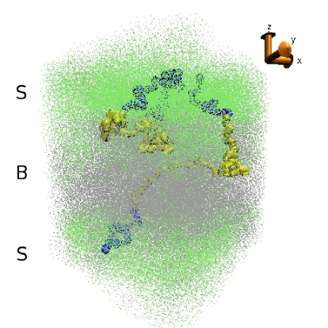
This one has then been applied in order to generate four types of triblocks according to the percentage of loop chains, namely $0\%$, $30\%$, $60\%$ and $100\%$. These loop chains are defined as chains that do not cross the entire material from a glassy phase $S$ to the opposite $S$ and by the way that also do not cross the whole rubbery phase $B$. Then, they loop back to their starting glassy phase while a part of the chain lies in the rubbery region. Such a chain is depicted in Fig. 1.

For each system, the number of obtained chains of desired length $N=200$ is respectively $M=192$, $M=188$, $M=194$ and $M=191$, and systems are kept under a $\langle P\rangle=0$ state after a run of $10^{6}$ MD steps. Finally, monomers dynamic in each phases has been checked by computing the incoherent intermediate scattering function $F_{s}(\mathbf{k},t)=\langle\frac{1}{N_{\alpha}}\sum_{j=1}^{N_{\alpha}}\exp{\left(i\mathbf{k}.\delta\mathbf{r}_{j}(t-t_{0})\right)}\rangle$ where $\delta\mathbf{r}(t-t_{0})=\mathbf{r}(t)-\mathbf{r}(t_{0})$, which depicts (not shown) a typical glassy behavior Bennemann99 in $S$ domains, and a rapid relaxation behavior in the rubbery $B$ domain.

In order to have a reference state, a homopolymer is also simulated using the $0\%$ configuration and setting $u^{0}_{\alpha\beta}=u^{0}_{SS}\equiv 1.0u^{0}$ this for all $(\alpha,\beta)$. A subsequent simulation run is performed during $10^{7}$ MD steps at $k_{B}T=0.3u^{0}_{SS}$ and $\langle P\rangle=0$ using the same anisotropic Nosé-Hoover barostat. After this run, the density of chain ends was checked to correspond to that of a directed homopolymer, namely, that chain ends are located in $z\sim 0$ and $z\sim L_{z}$. In the following, this directed homopolymer will be referred to as $hP$.

Finally, an isotropic homopolymer has also been generated by annealing the previous $hP$ polymer at $k_{B}T=1.0u^{0}_{SS}$ and $\langle P\rangle=0.5$ during $2\times 10^{7}$ MD steps, and cooling it to $k_{B}T=0.3u^{0}_{SS}$ for a time of $10^{6}$ MD steps. Then an additional run of $10^{6}$ MDS at the same temperature and pressure $\langle P\rangle=0$ has been performed. In this case, the density of chain ends was checked to be spatially homogeneous. In the following, we will refer to this sample as $iP$ polymer.

Glassy homopolymers and glassy phases in triblocks are then out of equilibrium. The $\alpha$ relaxation time $\tau_{\alpha}$ is defined as the time at which $F_{s}(\mathbf{k}_{1},\tau_{\alpha})=1/e$, where $\mathbf{k}_{1}$ is the first peak position in the structure factor. We found $\tau_{\alpha}$ of same order than the typical time used to perform the deformation experiment. In that sense, ageing effects may not significantly contribute to the glassy dynamics upon deformation, and are expected to not alter the mechanical response of the materials.

II.2 Boundary driven uniaxial tensile test

A method in which the deformation is applied first at boundaries and then is self-transmitted to the sample has been developed in order to mimic experiments Makke . The periodic boundary condition in the $z$-axis (direction of the applied deformation) is removed, while the other directions are kept periodic. Hence, chains that cross the periodic-image boundary in the $z$ direction were unwrapped and cut. This induces length polydispersity and then slightly decreases the total number of monomers per samples. For instance, it only alters the glassy parts of the triblocks. Another simulation run of $5\times 10^{6}$ MD steps is added to ensure all samples are still under an overall $\langle P\rangle=0$ state.

Grips are defined in the two glassy regions with a thickness of $2.6a_{SS}$, the upper one for $z>L_{z}-2.6a_{SS}$ and the lower for $z<2.6a_{SS}$. Then, forces and velocities are set to zero and $v_{0}$ respectively for all monomers lying in the grips, requesting a $v_{0}=0$ for lower grip. The lower grip is then coupled to an elastic spring with a force $\mathbf{F}^{l}=-K\left(\mathbf{r}^{l}_{cm}(t)-\mathbf{r}^{l}_{cm}(0)\right)$ adjusted so that the average lower grip velocity is null, as requested. The upper grip is also coupled to an elastic spring with a force also adjusted to preserve the requested upper grip velocity $v_{o}\mathbf{e_{z}}$, and is given by $\mathbf{F}^{u}=-K\left(\mathbf{r}^{u}_{cm}(t)-\mathbf{r}^{u}_{cm}(0)-v_{0}t\mathbf{e_{z}}\right)$. In both expressions, $\mathbf{r}_{cm}(t)$ denotes the center of mass position of grips at time $t$.

During this boundary driven deformation protocol, a Berendsen thermostat is used with a heat bath of $k_{B}T=0.3u^{0}_{\alpha\beta}$, while an anisotropic Nosé-Hoover barostat is applied in order to keep a lateral pressure $P_{xx}=P_{yy}=0$. The obtained deformation thus mimics a uniaxial tensile test. As discussed in Ref. Makke , the value of $K$ should be chosen as ten times as stiff as the initial sample, in order to lead to a numerically stable deformation scheme; such a condition is fulfilled in our numerical experiment.

sample code	$E_{Y}$	$G_{r}$	$\sigma_{flow}$	$\langle N_{e}\rangle$
$0\%$	$2.77$	$0.033$	$0.21$	$47$
$30\%$	$2.81$	$0.044$	$0.22$	$33$
$60\%$	$2.59$	$0.042$	$0.23$	$26$
$100\%$	$2.12$	$0.005$	$0.17$	$9$
$hP$	$13.4$	$0.27$	$0.42$	$60$
$iP$	$11.8$	$0.15$	$0.40$	$27$

Tab 1: Young’s modulus $E_{Y}$, hardening modulus $G_{r}$, and post-yield flow stress $\sigma_{flow}$ from stress-strain curve in Fig. 2, for all simulated systems. Also given, the average entanglement length $\langle N_{e}\rangle$ for undeformed samples and from the primitive path analysis.

II.3 Primitive Path Analysis

Several theories try to explain the deformation of polymer melts in both rubbery and glassy states. In the rubbery state, polymers can explore many conformations under the constraint of cross-link points (entanglements, covalent bonds…). Entropic-based classical theory of rubber elasticity Arruda1 ; Arruda2 ; Boyce , which neglects entanglements, may be used. However, in the glassy state, chains are slow down and may visit conformations in a noncontinuous way under deformation. This leads to stress dissipation effects Bocquet09 ; Hoy07 ; Hoy08 under deformation, noisy term currently not present in rubber elasticity theories.

Statistical mechanic theories improve the lack of cross-link effects by including entanglements to the constitutive relation via some additional terms Everaers96 ; Rubinstein02 , as well as by developing subnetwork deformation formalisms Rubinstein97 ; Uchida08 . It’s then supposed that entanglements depart from an initial distribution, while nothing more is said about its evolution upon deformation. This is a crucial point, as nothing compels polymer glasses and thermoplastic triblocks to not explore other sets of entanglement distributions.

Fig 2: (Color online) True stress $\sigma_{zz}$ measured during boundary driven tensile test against (a) true strain $\lambda=L_{z}(t)/L_{z}(0)$, and (b) Gaussian strain $g(\lambda)=\lambda^{2}-\lambda^{-1}$. Inset: Gaussian strain-hardening plot, in which stresses are normalized by $\sigma_{flow}$.

Under deformation, the stress-strain relation of these materials is expected to follow a superposition principle, with one contribution from inherent glassy structures and their contribution to energy landscape, leading to the so-called yield stress, and the other contribution from strain-hardening effects. Events from the latter may be related to thermally activated processes Haward93 ; Govaert04 ; Sarva07 ; Boyce90 , conformational effects McKechnie93 , or topological entanglement effects Vorselaars09 ; Fetters94 ; Fetters99 ; Lyulin05 . It was also shown in Hoy06 ; Uchida08 for a wide range of polymer glasses, that underlying entanglement effects contribute to the strain hardening.

The PPA framework Everaers04 ; Sukumaran05 furnishes a practical tool in order to identify the entanglements. Such an analysis has been performed on undeformed triblocks and $hP$ and $iP$ polymer glasses, averaging the number of monomers $N_{e}$ per Kuhn segment over all chains. Results are summarized in Tab. 1, in which it first appears for triblocks that $\langle N_{e}\rangle$ decreases with the increasing amount of loop chains, thus leading on the same manner to an increase of the entanglement density $\rho_{e}=\rho/2\langle N_{e}\rangle$. For polymer glasses, the entanglement density $\rho_{e}$ is higher for the isotropic $iP$ glass than for the directed $hP$ glass. This is also expected regarding to the average imposed chains conformations for the latter.

In order to study more precisely the evolution of entanglements during the tensile test numerical experiment, the PPA has been used every $10^{4}$ MD steps on dumped configurations, and $10^{4}$ times during the whole deformation process. For each dumped configuration to which PPA has been applied (hereinafter referred to PP chains), three quantities are extracted:

• for each PP polymer chain, the curvature between a monomer $i$ and its neighbors $j=i-\delta/2$ and $k=i+\delta/2$ is computed. The spatial position and monomer $Id$ where the bending angle is maximal is then stored. We refer to this ensemble as $MaxBend$, and $\delta=4$ is used in the following.

• according to a distance criterion $r_{l}\equiv\mu.r_{c}$, each monomer of a chain $1$ having another monomer of a chain $2$ at a distance less than $r_{l}$ is an element of the ensemble $Contacts$ for chains $1$ and $2$.

• a more restrictive ensemble per chain is built as the intersection of both previous ensembles. Entanglements taking part of this ensemble can be considered as $Mutual$ entanglements.

Both $Contacts$ and $Mutual$ ensembles depend on the value of the contact length $r_{l}=\mu.r_{c}$, with $\mu\in]0,\infty[$ and $r_{c}$ the cut-off distance in Eq.(1). Several values were tested. For $\mu<r_{c}^{-1}$, the distance criterion to build contacts is too restrictive, and the ensemble contains too few elements to perform a correct statistical analysis. In the limit of $\mu\rightarrow\infty$, one has $\mathcal{P}_{a^{+}/a^{-}}(\mu,t,t_{0})\rightarrow 0,\,\forall(t,t_{0})$ (see Sec. IV.1.1), as expected in this mean-field limit. We found optimal results for $\mu=r_{c}^{-1}$, and checked that varying it do not alter main results. This value will be used in the following.

Finally, from a computational point of view, the complete analysis, including parallel implementation of PPA on a $16$ processors computer and well optimized post-processing codes, took around $1300\,s$ CPU per dumped configuration.

III Response to deformation

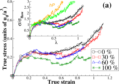
A uniaxial tensile test is performed at a temperature $k_{B}T=0.3u^{0}_{\alpha\beta}$ under anisotropic barostatic conditions $P_{xx}=P_{yy}=0$, with an applied upper grip velocity $v_{0}\mathbf{e_{z}}=10^{-4}a_{\alpha\beta}/\tau_{LJ}\mathbf{e_{z}}$. The true stress $\sigma_{zz}$ is monitored as a function of the elongation $\lambda=L_{z}(t)/L_{z}(0)$. Results are shown in Fig. 2(a) for all samples and versus the true strain $ln{(\lambda)}$. One can separate the stress-strain curve in three regions: (i) an elastic regime with possible localized irreversible monomer rearrangements Tanguy06 , (ii) a maximum $\sigma_{Y}$ which marks the onset of plasticity, directly followed by a strain softening regime, (iii) a quasi-ideal plastic flow $\sigma_{flow}$ and a strain hardening regime at large deformations. For triblocks, the first stage extends to strain less than $5-7\%$, while for $hP$ and $iP$ polymer glasses, this one covers the region with strain less than $2\%$. From this elastic regime, the Young’s modulus $E_{Y}$ is extracted, with higher values for polymer glasses compared to ones for triblocks. Results are given in Tab. 1.

The ratio of Young’s moduli for homopolymers to triblocks is in quantitative agreement with one observed experimentally Cohen00 . We also observe that Young’s modulus for directed polymer glass $hP$ is naturally higher than the one for the isotropic glass $iP$, for a deformation imposed along the $hP$ preferential chains average orientation. Depending the percentage of loop chains, different stiffness are observed for triblocks in the elastic regime. It appears that the $100\%$ loop seems to be weaker, while it is hard to conclude between other triblocks. Larger systems with several lamellae are needed to go further.

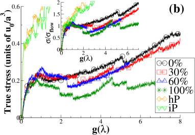
In Fig. 2(b), the true stress is also plotted in the Gaussian strain-hardening framework using the relation $\sigma=\sigma_{flow}+G_{r}g(\lambda)$, where $g(\lambda)=\lambda^{2}-\lambda^{-1}$. Fitting the stress-strain curves with this expression defines the hardening modulus $G_{r}$ and the offset yield stress $\sigma_{flow}$. Results are summarized on Tab. 1 for all systems. This kind of plot allows us to separate the plastic flow and stress-hardening regions for $g(\lambda)\gtrsim 1$, to the preyield one for $g(\lambda)\lesssim 0.8$. By this way, it also appears for triblocks that stress-strain curves seem to show two peaks around the yield zone.

In Figs. 2(a) and (b), we note different behaviors under deformation for triblocks and pure polymer glasses. The directed $hP$ glass displays a stronger strain-hardening than the isotropic $iP$ glass. Then polymer glasses have a stronger strain-hardening than triblocks. For triblocks, large stress drops appear suddenly and earlier when the amount of loop chains increases.

The presence of the elastomer also affects the response of triblocks. Instead of breaking, drops are nearly followed by local strain hardening zones, until another large drop appears, thus relaxing the stress in the whole material. This has an impact on chains orientation, mainly in the glassy phase, where a chevron-type structural change may occur Huy03 .

Fig 3: (Color online) Mean second Legendre polynomial $P_{2}$ between bond segments and applied deformation director $\textbf{e}_{z}$ upon deformation. $\langle P_{2}\rangle$ is plotted for triblocks, for chains in the rubbery phase, and on (inset), for chains in the glassy phase. Both plots are against the Gaussian strain $g(\lambda)=\lambda^{2}-\lambda^{-1}$. Also plotted is the Legendre polynomial for $hP$ and $iP$ homopolymers. The increase of $\langle P_{2}\rangle$ mimics the trend of polymer chain segments to align along to $\textbf{e}_{z}$, the direction of applied deformation.

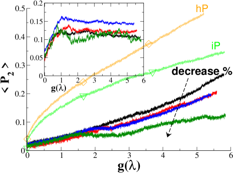
The orientation process of chains upon deformation can be monitored by the second Legendre polynomial $P_{2}=\frac{1}{2}\left(3\cos^{2}(\theta)-1\right)$, where $\theta$ is formed by the vector between monomers $[i,i+1]$ of the same chain and the direction of the applied deformation. The average orientation of the segments is taken as the ensemble average $\langle P_{2}\rangle$, where $\langle P_{2}\rangle=1$ means a tendency of chains to orient along the direction of the applied deformation, and $\langle P_{2}\rangle=0$ means an average random orientation of chains.

In Fig. 3, $\langle P_{2}\rangle$ is plotted, for triblocks, for monomers in the rubbery phase. Average chain orientation becomes weaker with the increase of the amount of loop chains. This is expected because of the average isotropic conformations of these chains. In the inset of the Fig. 3, an orientation process is activated in the glassy phase, until the yield point is reached around $g(\lambda)\sim 1$. After yield, glassy chains adopt an average different orientation that does not change anymore and with a strength that increases with the amount of loop chains. This tilting process is associated to a topological transition of conformations of glassy chains, due to the presence of discontinuities in the elastic medium of triblocks at the interfaces. The energy transferred to the material under the applied deformation leads to a localization of stresses (and/or specific monomer displacements) in the vicinity of the interfaces. This energy transferred to the glassy phase is strong enough after yield stress to cause an instability of the lamellae, leading to a transition from a lamellar to a chevron type structure Read99 .

Fig 4: (Color online) Spatially resolved distributions of entanglements from each ensemble (see Sec. II.3 for details) during deformation. Black lines represent the average position of the interfaces $S/B$ (for $z<0$) and $B/S$ (for $z>0$), and symbols are related to the considered ensemble. (a) For $0\%$ loop and (b) for $60\%$ loop triblocks.

We note that the $30\%$ and $60\%$ loop triblocks have a tendency to orient more in the glassy phase than the $0\%$ triblock. Thus the tilting process is more pronounced when the amount of loop chains increases, meaning that more energy is transferred trough the interface to the glassy phase. For the special case of the $100\%$ loop, large fluctuations are observed due to the higher capacity of chains to reorient. Furthermore, it clearly appears that the changes in trend of $\langle P_{2}\rangle$ in the rubbery phase can be well mapped onto the large stress drops in the stress-strain curve of Fig. 2(b). Hence, these ones find their origin in the release of topological constraints and average chain orientation.

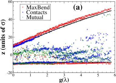
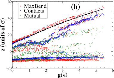
In Figs. 4(a) and (b), the time and space analysis of entanglements from ensembles $MaxBend$, $Contacts$ and $Mutual$, are plotted during the whole deformation process. In these figures, the black lines represent the average position of the interfaces between $S/B$ phases for $z<0.0$, and $B/S$ phases for $z>0.0$. For the $0\%$ loop triblock in Fig. 4(a), $MaxBend$ entanglements are mostly localized in the glassy regions, and in the vicinity of the interfaces. For the $60\%$ loop triblock in Fig. 4(b), another contribution appears in the rubbery phase, until the stress drop located at $g(\lambda)\sim 2$ (see Fig. 2) is reached and after which $MaxBend$ entanglements localize on both parts of the interfaces. $Contact$ entanglements probe the dynamics of relevant contacts between chains upon deformation. For both triblocks, relevant contacts disappear in the vicinity of the upper moving interface, nearby to the value of the yield point at $g(\lambda)\sim 1$. This lost of the interchain connectivity affects the balance with maximum curvature entanglements, then leading to a local interface morphology change, i.e. the chevron-type orientation transition.

For the $0\%$ loop triblock, these contacts persist in the rubbery phase and far from the moving interface. On the other way, they tend to be spatially distributed at a fixed distance from the moving interface for the $60\%$ loop triblock, and coincide with some maximum bending entanglements. This might be an effect of the loop chains, which preserve the material stiffness and stress transmission by adapting their conformations. It explains why strain-hardening for $30\%$ and $60\%$ loop triblocks is weakly dependent of the amount of loop chains, in regard to the $0\%$ loop triblock. On the other way, it is found (not shown) for $hP$ and $iP$ homopolymers that the same entanglement sets are well distributed over the whole simulation box.

Finally, we note that the ensemble $Mutual$, which is more restrictive, seems to be a good compromise in order to capture relevant entanglements. In the following, we will mainly focus on that ensemble.

IV Entanglements statistics

Using statistical ensembles for entanglements defined in the previous Sec. II.3, a specific attention is paid on the “participative dynamics” of these entanglements upon the tensile test numerical experiment depicted in Sec. III. To this aim, we split the contribution of these entanglements in two main contributions: from the initial distribution, and from the distributions on the fly.

IV.1 Contribution of initial entanglements

The initial distributions of entanglements form the initial networks of triblocks and polymer glasses. For their representation, we define the matrix $\underline{\underline{\mathbf{\Omega}}}_{t}$ of distributions of events from the $Mutual$ ensemble set at time $t$. This matrix has $M$ rows and each row represents a chain of $N$ monomers. Element of a row is equal to $0$ when the monomer $i$ is not an element of the considered ensemble and $1$ otherwise.

IV.1.1 Creation vs annihilation

We first define $a^{+}(\mu,t,t_{0})$ as the number of events present at time $t$ but not at time $t_{0}$ divided by the size of the ensemble set at time $t$ times the amount of time $(t-t_{0})$, thus characterizing the rate of created events at this time. Using the above representation:

$$a^{+}(\mu,t,t_{0})=\frac{1}{(t-t_{0})N_{t}}\mathrm{Tr}\left(\mbox{$\underline{\underline{\mathbf{\Omega}}}_{t}$}\cdot\mbox{${}^{T}\underline{\underline{\mathbf{\widetilde{\Omega}}}}_{t_{0}}$}\right)$$ (3)

where $N_{t}$ is the size of the ensemble set at time $t$ and ${}^{T}\underline{\underline{\mathbf{\widetilde{\Omega}}}}_{t_{0}}$ contains complementary elements (Boolean $NOT$) with respect to the universe $(0,1)$ for each state defining a monomer in the transposed matrix ${}^{T}\underline{\underline{\mathbf{\Omega}}}_{t_{0}}$ of $\underline{\underline{\mathbf{\Omega}}}_{t_{0}}$. Hence, the operation $\widetilde{\mathcal{O}}:\mbox{$\underline{\underline{\mathbf{\Omega}}}_{t_{0}}$}\longrightarrow\mbox{$\underline{\underline{\mathbf{\widetilde{\Omega}}}}_{t_{0}}$}$ is related to the Boolean $NOT$ transformation applied to elements of each row. In practice, if a monomer of a chain has a state $0$ in a row of $\underline{\underline{\mathbf{\Omega}}}_{t_{0}}$ at $t_{0}$, then such a monomer will have a value $1$ in the column of the associated transposed matrix ${}^{T}\underline{\underline{\mathbf{\widetilde{\Omega}}}}_{t_{0}}$.

Fig 5: (Color online) Relative ratio $\mathcal{P}_{a^{+}/a^{-}}(\mu,t,t_{0})$ of created vs annihilated entanglements during the whole deformation process. Events are taken from the initial $Mutual$ entanglements set. Main panel: results for triblocks. Inset: same ratio for the $iP$ and $hP$ polymer glasses. The dashed line represents the yield point for these glasses.

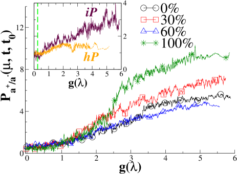
Conversely, we define $a^{-}(\mu,t,t_{0})$ as the number of events present at time $t_{0}$ but not at time $t$ and also divided by the size of the ensemble set at time $t$ times the time length $(t-t_{0})$, thus characterizing the rate of annihilated events at measuring time. In a more compact notation, one has:

$$a^{-}(\mu,t,t_{0})=\frac{1}{(t-t_{0})N_{t}}\mathrm{Tr}\left(\mbox{$\underline{\underline{\mathbf{\widetilde{\Omega}}}}_{t}$}\cdot\mbox{${}^{T}\underline{\underline{\mathbf{\Omega}}}_{t_{0}}$}\right)$$ (4)

where $\underline{\underline{\mathbf{\widetilde{\Omega}}}}_{t}$ contains complementary elements (Boolean $NOT$) with respect to $(0,1)$ for each state defining a monomer in the matrix $\underline{\underline{\mathbf{\Omega}}}_{t}$. Thus, if a monomer of a chain has a state $0$ in a row of $\underline{\underline{\mathbf{\Omega}}}_{t}$, it will become $1$ in the same row of $\underline{\underline{\mathbf{\widetilde{\Omega}}}}_{t}$.

The quantities Eq.(3) and Eq.(4) may differ during the deformation, leading to an asymmetric creation-annihilation process. The ratio $\mathcal{P}_{a^{+}/a^{-}}(\mu,t,t_{0})$ captures such a process.

In Fig. 5, the variation of the ratio $\mathcal{P}_{a^{+}/a^{-}}(\mu,t,t_{0})$ is plotted for the $Mutual$ ensemble set of entanglements. For triblocks, and before yield at $g(\lambda)\sim 1$, balance between alive and created events is achieved with regard to the initial entanglements set. Then after yield, more and more new events are created, which unbalances the ratio with annihilated ones, then leading to an asymmetric creation-annihilation process of entanglements. It coincides with the chevron-type transition in the inset of Fig. 3 that allows glassy chain ends to release some topological constraints. The asymmetric process has an higher magnitude in the case of the $100\%$ loop sample, with changes in slope that also correspond to the large drops appearing in the stress-strain curve in Fig. 2.

After yield, these more created or activated events can be seen as the result of “cascades” of disentanglements of older events, where such processes alter chain conformation and, this, in order to maintain the rigidity of the system. It means that the $100\%$ loop triblock is more affected by the deformation in the plastic flow regime than other triblocks and needs to explore more chain conformations in order to preserve a mechanical stability.

Intriguingly, it appears that the $30\%$ loop triblock follows the same trend when compared to the $60\%$ loop one. The latter is indeed closer to the $0\%$ loop behaviour. A lower balance is then achieved for this triblock, which means that it is not forced to explore more and more new sets and destroy older ones in order to preserve its mechanical stability. In that sense, this amount of loop chains seems to much preserve the triblock integrity, and plays in favour of the future metastable states during the deformation. This can be related to the more pronounced chevron-type process for this triblock, which compensates the loss of topological constraints due to the low amount of crossing chains. A this point, a more precise study is needed to explore this compensation effect, and how this one depends on the amount of loop chains.

In the inset of Fig. 5, the ratio $\mathcal{P}_{a^{+}/a^{-}}(\mu,t,t_{0})$ is plotted for the $iP$ and $hP$ polymer glasses. Before yield, balance between created and annihilated events is observed, followed after yield by an asymmetric process. Its magnitude for the $iP$ glass is higher than the one for the directed $hP$ glass, because new metastable topological intermediate configurations are more accessible for $iP$. Despite of the glassy state, and under deformation, energetic barriers have then an higher probability to be crossed, leading to this higher ratio. Finally, the ratio $\mathcal{P}_{a^{+}/a^{-}}(\mu,t,t_{0})$ for $iP$ and $hP$ glasses is also weaker than the one for triblocks. It is mainly due to the presence of a rubbery region in triblocks, in which chains can explore more conformations.

IV.1.2 Survival events

Additionally, we define the distribution $\mathcal{P}_{s}(\mu,t,t_{0})$ of $Mutual$ survival events between initial time $t_{0}$ and the measuring time $t$ during deformation. Using the same formalism for Eqs.(3) and (4), it can be written:

$$\mathcal{P}_{s}(\mu,t,t_{0})=\frac{1}{N_{t}}\mathrm{Tr}\left(\mbox{$\underline{\underline{\mathbf{\Omega}}}_{t}$}\cdot\mbox{${}^{T}\underline{\underline{\mathbf{\Omega}}}_{t_{0}}$}\right)$$ (5)

Such a distribution is plotted in Fig. 6. It clearly appears two distinct regimes with increasing $g(\lambda)$: a plateau until yield strain is reached, followed by a power law decrease of survival events $\mathcal{P}_{s}(\mu,t,t_{0})\sim g(\lambda)^{-\beta}$. For triblocks, $\beta\approx 0.83,\,0.74,\,0.68,\,0.97$ for $0,\,30,\,60$ and $100\%$ loop chains respectively. Hence, for the three first triblocks, the plateau value before yield is quantitatively the same. Except the $100\%$ loop triblock, the rate of loss of the contribution of initial mutual entanglements after yield decreases with the increase of the amount of loop chains. The triblock with the lowest amount explores more rapidly new entanglements set on deformation than ones with a higher amount; loop chains offer a longer memory effect of the initial mutual entanglements network.

Fig 6: (Color online) Distribution $\mathcal{P}_{s}(\mu,t,t_{0})$ of survival events between initial undeformed state $t_{0}$ and deformation time $t$. Events are part of the $Mutual$ ensemble set of entanglements, and data are plotted for triblocks. The $30\%$ loop chains triblock is omitted for clarity. Inset: same quantity for $hP$ and $iP$ polymer glasses. The vertical dashed line marks the onset of plastic flow.

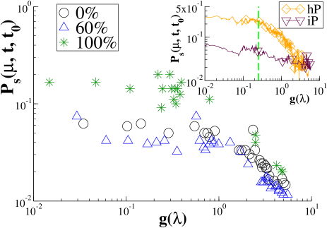
The plateau can be interpreted as the fact that initial $Mutual$ entanglements mainly contribute to the elastic linear (and nonlinear) part of the strain-stress curve, while their contribution to the plastic flow and strain-hardening regime decreases with increasing strain. An higher preyield “plateau” is observed for the $100\%$ loop chain triblock, in which chains more preserve the initial network of mutual entanglements, but on counterpart make the material stiffer and more sensible to high deformations. An higher postyield power-law exponent is also measured for this triblock, which means that this material needs to explore new states more rapidly.

Finally, in the inset of Fig. 6, Eq. (5) is plotted for the $hP$ and $iP$ glasses. Due to their chain average orientation, the preyield regime depicts a higher survival magnitude for the directed glass than for the isotropic one. In the postyield regime, the power law behavior is fitted with an exponent $\beta\approx 1.01$ for $hP$ polymer glass, and $\beta\approx 0.2$ for $iP$ glass. The rate of loss of initial mutual entanglements is then higher for the directed glass than for the isotropic one. It is because, given the initial $hP$ glass entanglement network, the chain average orientations are too constraining to expect a mechanical equilibrium in the postyield regime. This glass needs to explore new mutual entanglement states more rapidly upon deformation than the isotropic one.

IV.2 Contribution of on the fly entanglements

The participative dynamics of mutual entanglements is evaluated by monitoring the contribution of their distributions to the current deformation time $t$, given a spanning time $\Delta^{\ast}$. To this aim, we define the retarded distribution $\mathcal{P}_{s}(\mu,\Delta^{\ast})$ of survival events between time $t$ and a new origin $\widetilde{t_{0}}=t-\Delta^{\ast}$. This distribution can be written using the same formalism as for Eq.(5):

$$\mathcal{P}_{s}(\mu,\Delta^{\ast})=\frac{1}{N_{t}}\mathrm{Tr}\left(\mbox{$\underline{\underline{\mathbf{\Omega}}}_{t}$}\cdot\mbox{${}^{T}\underline{\underline{\mathbf{\Omega}}}_{\Delta^{\ast}}$}\right)$$ (6)

In Eq.(6), the quantity ${}^{T}\underline{\underline{\mathbf{\Omega}}}_{\Delta^{\ast}}$ is then related to the matrix of distribution of mutual entanglements at a given origin $\Delta^{\ast}$. The distribution $\mathcal{P}_{s}(\mu,\Delta^{\ast})$ is plotted in Fig. 7 for the different $SBS$ triblocks and their amount of loop chains, i.e. from $0\%$ to $100\%$, versus the Gaussian strain $g(\lambda)=\lambda^{2}-\lambda^{-1}$ and $\lambda=L_{z}(t)/L_{z}(0)$.

Fig 7: (Color online) Distribution $\mathcal{P}_{s}(\mu,\Delta^{\ast})$ of survival events between deformation times $t$ and $t-\Delta^{\ast}$. Events are part of the $Mutual$ ensemble set of entanglements, and distributions are plotted for triblocks with specified percentage of loop chains. The parameter $\Delta^{\ast}$ is given in $\tau_{LJ}$ units. Exponents $\alpha$ and $\gamma$ that characterize the two regimes discussed in the text are also drawn. The vertical dashed line marks the yield point.

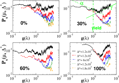
In Fig. 7, the “probe” times $\Delta^{\ast}$ are given in $\tau_{LJ}$ units, with all $\Delta^{\ast}<t_{tot}/2$ and the total amount of simulation time $t_{tot}=6\times 10^{5}\tau_{LJ}$ for all simulated systems. Values of the probe times are taken according to specific deformation zones of the stress-strain curves in Fig. 2. For the elastic zone, where $t_{elastic}$ is an estimate of the upper time for the elastic limit, we have $\Delta^{\ast}=1.2\times 10^{3},\,1.2\times 10^{4}<t_{elastic}$. The value $\Delta^{\ast}=6\times 10^{4}$ is chosen to lie between $t_{p1}$ and $t_{p2}$, which are estimates of the deformation time associated with the two peaks in the yielding zone of the stress-strain curve. Finally, both values $\Delta^{\ast}=1.2\times 10^{5},\,1.8\times 10^{5}>t_{hard}$, where $t_{hard}$ is the time after which strain-hardening occurs.

It appears in Fig. 7 before yield and $\Delta^{\ast}<t_{elastic}$, that distributions have a lower magnitude when the amount of loop chains increases, except for $100\%$ loop. If loop chains maintain the initial set of entanglements, the $0\%$ triblock is more stable than other triblocks with regard to new on the fly entanglement sets. The $100\%$ loop triblock depicts higher distributions, which is a direct effect of the special amount of these chains as already discussed in Sec. IV.1.

The $\mathcal{P}_{s}(\mu,\Delta^{\ast})$ curves seem to follow a master curve which can be split in three parts: (1) a plateau for $\Delta^{\ast}<t_{elastic}$, which stays until the yield strain at $g(\lambda)\sim 1$ is reached, (2) a power law decrease fitted with an exponent $\alpha$, and (3) a power low increase also expressed in terms of an exponent $\gamma$. The transition from the $\alpha$ to $\gamma$ regime gives rise to a minimum, which we denote $\mathit{min}\{\mathcal{P}_{s}(\mu,\Delta^{\ast})\}$.

Events in the $\alpha$ regime are related with initial events from the preyield zone, and quantify their contributions to events moving away from the yield point. The minimum $\mathit{min}\{\mathcal{P}_{s}(\mu,\Delta^{\ast})\}$ is related to the contribution of events at yield point to postyield ones. Finally, the $\gamma$ regime characterizes the contribution of events from the post-yield region to ones in the strain-hardening regime. Hence, an increase of the contributions in this regime marks the emergence of long-time correlations and memory effects.

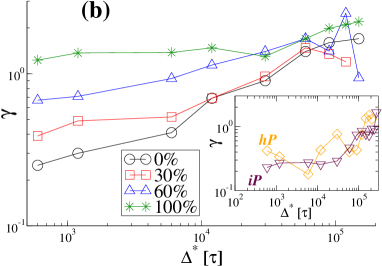
In the $\gamma$ regime, the distributions of survival mutual entanglements separated by the shortest $\Delta^{\ast}$ have a higher magnitude than ones for longer $\Delta^{\ast}$. On counterpart, the route to the memory effect is less pronounced for small probe times $\Delta^{\ast}$ than in the case of larger probe times if we relate this route to the $\gamma$ exponent. Thus, at larger probe times, survival distributions between postyield and in-strain-hardening entanglements tend to higher magnitudes more “rapidly” upon deformation. Finally, these trends in the $\gamma$ regime are also more and more pronounced when the amount of loop chains increases, as it is shown in Fig. 8(b), where the ”memory” exponent $\gamma$ is plotted against the probe time. Consequently, memory effects and long time correlations between sets of mutual entanglements are more and more important in the postyield regime, and the loop chains reinforce the memory effects.

Fig 8: (Color online) Variation of $\alpha$ (a) and $\gamma$ (b) exponents depicted in Fig. 7 against the probe time $\Delta^{\ast}$ that separates two measuring times upon deformation. Exponents characterize the two power-law behaviors for $\mathcal{P}_{s}(\mu,\Delta^{\ast})$. On both main panels, data are plotted for triblocks, and on insets for $hP$ and $iP$ polymer glasses.

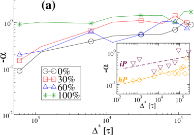
In Fig. 8(a), the increase of $|\alpha|$ with $\Delta^{\ast}$ denotes an increase of the loss of the contribution of preyield mutual entanglements to postyield ones. Thus, long-time correlations become weaker and weaker between the sets of mutual entanglements from these two regimes. The values of $|\alpha|$ for the $100\%$ loop triblock are also higher, especially for $\Delta^{\ast}<t_{p1,p2}$, which points out that this triblock experiences more chain conformations than others.

Exponents $\alpha$ and $\gamma$ for the polymer glasses are plotted in the insets of respectively Figs. 8(a) and (b). For the isotropic glass, the loss exponent $\alpha$ is higher than for the directed glass. It is because intermediate conformation states are more accessible for the isotropic glass, and thus it can explore more mutual entanglement sets. The slope of $|\alpha|$ with respect to $\Delta^{\ast}$ is also lower when compared to triblocks, because of the pure glassy state that slows down the debonding.

Finally, the memory exponent $\gamma$, which characterizes the postyield to strain-hardening contributions of sets of mutual entanglements, depicts, in Fig. 8(b), a common trend for both polymer glasses. With the increase of the probe time $\Delta^{\ast}$, it then appears that memory effect and long-time correlations become stronger. This trend seems to be more pronounced than for triblocks, which is again due to the pure glassy state.

V Concluding remarks and outlooks

During this study, an isotropic, a directed polymer glass and lamellar directed triblock copolymers were generated. The directed triblocks were developed in order to mimic the mechanical behavior of glassy/rubbery/glassy nanostructurated materials in the strong segregation regime. By tuning the amount of uncrossing or loop chains, it was possible to simulate different glassy/rubbery interface definitions. Material mechanical properties were investigated using a boundary driven tensile test experiment.

Using this methodology, the impact of loop chains on the mechanical response of triblocks has been approached. Their stress-strain curves depict large stress drops that come earlier upon deformation, with the increase of the amount of loop chains. A chevron-type transition is also observed, with a strength that increases with the same amount. Besides this facts, the global mechanical properties seem to not be deeply altered by these amounts, so that, it is hard to predict a critical amount of loop chains above which triblocks integrity is achieved. To overcome this fact, larger systems with repeated lamellar units should be considered in order to improve statistics, decrease fluctuations and reach a self-averaging regime.

The sets of mutual entanglements between chains were monitored during deformation, using a primitive path algorithm. A specific attention has been paid to the study of their statistics.

Given the initial undeformed sets of mutual entanglements, the evolution of the ratio of created over annihilated events, as well as the distributions of survival events, has been monitored. It has been shown that these quantities follow the two main parts of the stress-strain curve, namely, the preyield and postyield regimes. Monitoring on the fly sets of entanglements during the deformation allowed us to also approach the internal metastable cross-link states.

It appears that during the strain-hardening regime, the debonding of the initial mutual entanglement network occurs. Debonding of on the fly entanglement sets is correlated in time, depending the initial time window from which depart these sets. If one considers sets from the preyield regime, their contributions to the postyield regime decrease with a power-law behavior denoted by a loss exponent $\alpha$. On the other way, ones that depart from the postyield regime depict memory effects in the strain-hardening regime. In that case, a power-law behavior is observed, which is characterized by a memory exponent $\gamma$. The same trends occur for polymer glasses as well as for triblocks.

For triblocks with a non-null amount of crossing chains, the lower the amount is, the longer the memory effect of initial undeformed sets of mutual entanglements is. On the same way, loop chains also enhance long-time correlations and memory effects of internal metastable cross-link states continuously explored upon deformation.

Finally, it should be noted that the results obtained may depend on the applied strain rate. Further works should be employed in order to quantify this dependence.

The methodology developed during this study gives rise to further insights. First, the created and activated sets of mutual entanglements emerge from a complex process, which could contribute to new stable intermediate conformations as well as to participate to destabilization processes and related unstable states. The inner mechanisms of propagation of these ensemble sets should be more precisely studied, and especially how the large stress drops in Fig. 2 could be interpreted in terms of entanglements and how the amount of loop chains compensates the loss of topological constraints, as observed in Fig.5. With the methodology developed in this study, one could access these localized or delocalized (long-range) processes. A quasistatic protocol could be suitable in order to remove the thermally activated processes and distinguish the transmission mechanisms.

Furthermore, this methodology allowed us to deal with the problematic of the way external forcing is “internalized” by the systems via the cross-link process. The rheological response of these systems involves permanent cross-linked and uncross-linked sets, which can be described by some surviving probabilities $\zeta(t)$, until $t$ times of deformation occur after cross-linking. These states hold internal stresses. Under external forcing, they are metastable and require far from equilibrium operations in order to be created. In the studied systems, which depict rubbery phase or “interchain” connectivities, the generation of internal states as metastable states is closely related to the notion of plasticity. This notion is itself related, probably among many others, to some time scale competitions that take place during this generation process. This may lead to an instantaneous momentarily decrease of time scales, leading to a bias in favor of the future metastable state. Then, it would be also interesting to extend the notion of entanglement sets to the study of internal stress dissipation mechanisms and local displacement fields.

References

- (1) R. Seguela and J. Prud’homme, Macromolecules 14, 197 (1981).
- (2) Y. Cohen, R.J. Albalak, B.J. Dair, M.S. Capel, and E.L. Thomas, Macromolecules 33, 6502 (2000).
- (3) D. Kaelble, E. Cirlin, J Polym. Sci., Polym. Symp. 43, 131 (1973).
- (4) Y.D.M. Chen, R.E. Cohen, J. Appl. Polym. Sci. 21, 629 (1977).
- (5) G. Holden, E.T. Bishop, N.R. Legge, J. Polym. Sci. C: Polym. Symp. 26, 37 (1969).
- (6) T.A. Huy, R. Adhikari, and G.H. Michler, Polymer 44, 1247 (2003).
- (7) D.J. Read, R.A. Duckett, J. Sweeney, and T. McLeish, J. Phys. 32, 2087 (1999).
- (8) K. Kremer and G.S. Grest, J. Chem. Phys. 92, 5057 (1990).
- (9) J. Gao, J. Chem. Phys. 102, 1074 (1995).
- (10) M. Perez, O. Lame, F. Leonforte, and J.-L. Barrat, J. Chem. Phys. 128, 234904 (2007).
- (11) A. Makke, M. Perez, O. Lame, and J.-L. Barrat, J. Chem. Phys. 131, 014904 (2009).
- (12) C. Bennemann, J. Baschnagel and W. Paul, Eur. Phys. J. B 10, 323 (1999).
- (13) E.M. Arruda and M.C. Boyce, J. Mech. Phys. Solids 41, 389 (1993).
- (14) E.M. Arruda, M.C. Boyce, and H. Quintus-Bosz, International Journal of Plasticity 9, 783 (1993).
- (15) M.C. Boyce and E.M. Arruda, Math. and Mech. of Solids 6, 641 (2001).
- (16) L. Bocquet, A. Colin, and A. Adjari, Phys. Rev. Lett. 103, 036001 (2009).
- (17) R.S. Hoy and M.O. Robbins, Phys. Rev. Lett. 99, 117801 (2007).
- (18) R.S. Hoy and M.O. Robbins, Phys. Rev. E 77, 031801 (2008).
- (19) A. Tanguy, F. Leonforte, and J.-L. Barrat, Eur. Phys. Journal E 20, 355 (2006).
- (20) R.N. Haward, Macromolecules 26, 5860 (1993).
- (21) L.E. Govaert and T.A. Tervoort, J. Polym. Sci.:Polym. Phys. 42, 2041 (2004).
- (22) S.S. Sarva, S. Deschanel, M.C. Boyce, and W.N. Chen, Polymer, 48, 2208 (2007).
- (23) M.C. Boyce and E.M. Arruda, Polym. Eng. Sci., 30, 1288 (1990).
- (24) R. Everaers and K. Kremer, Phys. Rev. E 53, R37 (1996).
- (25) M. Rubinstein and S. Panyukov, Macomolecules 35, 6670 (2002).
- (26) M. Rubinstein and S. Panyukov, Macomolecules 30, 8036 (1997).
- (27) N. Uchida, G.S. Grest, and R. Everaers, J. Chem. Phys. 128, 044902 (2008).
- (28) J.I. McKechnie, R.N. Haward, D. Brown, and J.H.R. Clarke, Macromolecules 26, 198 (1993).
- (29) B. Vorselaars, A.V. Lyulin, M.A.J. Michels, J. Chem. Phys. 130, 074905 (2009).
- (30) R.S. Hoy and M.O. Robbins, J. Polym. Sci.:Polym. Phys. 44, 3487 (2006).
- (31) L.J. Fetters, D.J. Richter, T.A. Witten, and A. Zirkel, Macromolecules 27, 4639 (1994).
- (32) L.J. Fetters, D.J. Richter, S.T. Milner, and W.W Graessley, Macromolecules 32, 6847 (1999).
- (33) A.V. Lyulin, B. Vorselaars, M.A. Mazo, N.K. Balabaev, and M.A.J. Michels, Europhys. Lett. 71, 618 (2005).
- (34) R.S. Hoy and M.O. Robbins, Phys. Rev. E 72, 061802 (2005).
- (35) R. Everaers, S.K. Sukumaran, G.S. Grest, C. Svaneborg, A. Sivabramanian, and K. Kremer, Science 303 823 (2004).
- (36) S.K. Sukumaran, G.S. Grest, K. Kremer, and R. Everaers, J. Polym. Sci. Part B: Polym. Phys. 43, 917 (2005).