Population genetics in compressible flows

Abstract

We study competition between two biological species advected by a compressible velocity field. Individuals are treated as discrete Lagrangian particles that reproduce or die in a density-dependent fashion. In the absence of a velocity field and fitness advantage, number fluctuations lead to a coarsening dynamics typical of the stochastic Fisher equation. We then study three examples of compressible advecting fields: a shell model of turbulence, a sinusoidal velocity field and a linear velocity sink. In all cases, advection leads to a striking drop in the fixation time, as well as a large reduction in the global carrying capacity. Despite localization on convergence zones, one species goes extinct much more rapidly than in well-mixed populations. For a weak harmonic potential, one finds a bimodal distribution of fixation times. The long-lived states in this case are demixed configurations with a single boundary, whose location depends on the fitness advantage.

Challenging problems arise when spatial migrations of species are combined with population genetics. The population dynamics of a single species expanding into new territory was first studied in the pioneering works of Fisher, Kolmogorov, Petrovsky and Piscounov (FKPP) 1 ; 2 ; 3 . Later, Kimura and Weiss studied individual-based counterparts of the FKPP equation 6 , revealing the important role of number fluctuations. In particular, stochasticity is inevitable at a frontier, where the population size is small and the discrete nature of the individuals becomes essential. Depending on the parameter values, fluctuations can produce radical changes with respect to the deterministic predictions 3 ; 4 . If $f(x,t)$ is the population fraction of, say, a mutant species and $1-f(x,t)$ that of the wild type, the stochastic FKPP equation reads in one dimension 8 :

$$\partial_{t}f(x,t)=D\partial^{2}_{x}f+sf(1-f)+\sqrt{D_{g}f(1-f)}\xi(x,t)$$ (1)

where $D$ is the spatial diffusion constant, $D_{g}$ is the genetic diffusion constant (inversely proportional to the local population size $N_{l}$), $s$ is the genetic advantage of the mutant and $\xi=\xi(x,t)$ is a Gaussian noise, delta-correlated in time and space that must be interpreted using Ito calculus 8 ; 9 .

However, many species, from the distant past 11 up to the present, have competed in liquid environments, such as lakes, rivers and oceans. Interesting new phenomena arise when population dynamics is coupled to hydrodynamic flows 5 . For example, satellite observations of chlorophyll concentrations have identified long lived, segregated patches of marine microorganisms off the eastern coast of the southern tip of South America 12 , where species domains are largely determined by the tangential velocity field obtained from satellite altimetry. In cases such as these, the dynamics takes place in the presence of advecting flows, some of them at high Reynolds numbers 13 . It is often appropriate to consider a compressible velocity field, both because of inertial effects 14 associated with fairly large microorganisms (diameter 5-500$\mu$m), and because photosynthetic bacteria and plankton often control their buoyancy to stay close to the ocean surface 15 . In the latter case, the coarse-grained velocity field advecting the microorganisms will contain a compressible component to account for downwellings 16 . Recent works studied the dynamics of a single population in the presence of a compressible turbulent velocity field in one and two dimensions 17 ; 18 . Here, the interplay between turbulent dynamics and population growth leads to “quasilocation” on convergence zones and a remarkable reduction in the carrying capacity.

The study of competition in a hydrodynamics context, where both a compressible velocity field and stochasticity due to finite population sizes are present, calls for a nontrivial generalization of Eq. (1). One complication is that, because of compressibility, the sum of the concentrations of the two species is no longer invariant during the dynamics. Thus, we must clarify the definition of $f(x,t)$, the fraction of one particular species. A biologically important issue arises from overshooting: the density $f(x,t)$ can exceed unity near velocity sinks, resulting in an unphysical imaginary noise amplitude in Eq. (1).

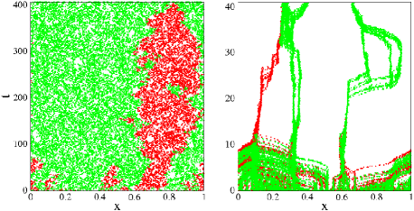
In this Letter, we overcome these problems by introducing a new model, designed to explore, for the first time, how compressible velocity flows affect the competition between two different species which can die and reproduce via cell division. In absence of an advecting field, the model reproduces the coarsening dynamics of spatial population genetics, as shown for one spatial dimension in Fig. 1a. Of particular importance in population genetics is the fixation time $\tau_{f}$, defined as the average time needed for one of the two species to reach extinction. The value of $\tau_{f}$ is proportional to the total population size in mean field approximation (i.e. assuming uniform spatial mixing) and grows to $L^{2}/D$ for a one dimensional system 8 . Conversely, Fig. 1b shows a typical simulation with our model using a high Reynold number synthetic velocity field extracted from a shell model of turbulence 17a . In striking contrast to the result without advecting flows (Fig. 1a and Ref. 8 ), one now finds competitions carried out on transient but persistent sinks in the velocity field. We find that turbulence not only compresses and reduces the overall population density, it also greatly reduces the fixation time $\tau_{f}$. Despite quasi-localization onto velocity sinks, the typical fixation time is much shorter than if particles were well mixed. We have also considered a compressible sinusoidal velocity field and a confining sink arising from a linear velocity profile. Remarkably, we find that these low Reynolds number compressible flows can also dramatically reduce fixation times. In the following, we investigate this phenomenon and propose a phenomenological explanation.

Eq. (1) is derived by assuming a fixed total concentration of individuals, so that if $f(x,t)$ is the concentration of one species, the other will have a concentration exactly equal to $1-f(x,t)$. To describe cases in which the total concentration can change due to an advecting flow, we introduce an off-lattice model in which two different organisms, $A$ and $B$, advect and diffuse in space, while undergoing duplication (i.e. cell division) and density-dependent annihilation (death). Specifically, we implement the following reactions: each particle of species $i=A,B$ duplicates with rate $\mu_{i}$ and annihilates with a rate $\bar{\mu}_{i}\widehat{n}_{i}$, where $\widehat{n}_{i}$ is the number of neighboring particles (of both types) in an interaction range $\delta\propto 1/N$, and $N$ is the total number of organisms that can be accomodated in the unit interval with total density $c_{A}+c_{B}=1$. To reduce the number of parameters, we set $\bar{\mu}_{A}=\bar{\mu}_{b}=\mu_{B}=\mu$, but take $\mu_{A}=\mu(1+s)$ to allow the possibility of a selective advantage (faster reproduction rate) of species $A$. We will start by analyzing in depth the neutral case $s=0$ and consider the effect of $s>0$ in the end of the Letter. In one dimension, our macroscopic coupled equations for the densities $c_{A}(x,t)$ and $c_{B}(x,t)$ of individuals of type $A$ and $B$ in an advecting field $v(x,t)$ read

$$\partial_{t}c_{A}\!\! =\!\! \!-\partial_{x}(vc_{A})\!+\!D\partial^{2}_{x}c_{A}\!+\!\mu c_{A}(1\!+\!s\!-\!c_{A}\!-\!c_{B})\!+\!\sigma_{A}\xi$$

$$\partial_{t}c_{B}\!\! =\!\! \!-\partial_{x}(vc_{B})\!+\!D\partial^{2}_{x}c_{B}\!+\!\mu c_{B}(1\!-\!c_{A}\!-\!c_{B})\!+\!\sigma_{B}\xi^{\prime}\$$ (2)

with $\sigma_{A}=\sqrt{\mu c_{A}(1+s+c_{A}+c_{B})/N}$ and $\sigma_{B}=\sqrt{\mu c_{B}(1+c_{A}+c_{B})/N}$. As discussed in suppl , for an interval of size $L$, let $N^{-1}\rightarrow L/N=\delta/N_{l}$, where $N_{l}$ is the local carrying capacity of a region of size $\delta$. $\xi(x,t)$ and $\xi^{\prime}(x,t)$ are independent delta-correlated noise sources with an Ito-calculus interpretation as in Eq. (1), and we have rescaled the particle densities so that the local carrying capacity is $1$ when $v=s=0$. Although $s=0$ may seem nongeneric in the context of dynamical systems theory, this is a case of particular interest in population genetics, where it corresponds to the neutral theory of Kimura 6 .

Figure 1: Space-time plot of the off-lattice particle model, (a) no advecting velocity field and (b) with a compressible turbulent velocity field. Simulations are run until fixation (disappearance of one of the two species); note the reduced carrying capacity and the much faster fixation time in (b). Parameters values: $N=10^{3}$, $D=10^{-4}$, $\mu=1$. Parameters of the shell model are as in 17 .

The above equations follow from a microscopic master equation via the Kramers-Moyal method suppl , at this order equivalent to Van Kampen inverse system size expansion 20 . Multi-species versions of the FKPP equations have been already considered in Refs 21 , but not in the presence of an advecting field or number fluctuations.

We first simulated the particle model directly for $v=s=0$, finding a dynamics similar to that of the stochastic FKPP equation, Eq. (1), for $s=0$, see Fig.(1a). In this simple limit, our model can be considered as a grandcanonical generalization of Eq (1), where the total density of individuals $c_{A}+c_{B}$ is now allowed to fluctuate around an average value $1$. Details of the numerical implementation and the role of density fluctuations are presented in suppl . Hereafter, we fix the following parameters: $N=10^{3}$, $D=10^{-4}$, $\mu=1$ and $L=1$ where $L$ is the one dimensional domain endowed with periodic boundary conditions. With these parameters, $\tau_{f}$ would be $\sim 10^{4}$ for the one dimensional FKKP equation, and $\sim 10^{3}$ for the well-mixed case.

Introducing a compressible velocity field $v(x,t)$, as shown in Fig.(1b), leads to radically different dynamics. Individuals tend to concentrate at sinks in the velocity field. Further, competition is enhanced and the total number of individuals $n(t)$ present at time $t$ is on average significantly smaller than the total carrying capacity $N$. We implemented three different velocity fields: 1) a velocity field $v(x,t)$ generated by a shell model of compressible turbulence 17a ; 17 , reproducing the power spectrum of a high Reynolds number turbulent velocity field of forcing intensity $F$ suppl , 2) a static sine wave, $v(x)=F\sin(2\pi x)$, and 3) a linear velocity profile, $v(x)=-kx$, confining particles near the origin. Periodic boundary conditions on the unit interval are used in cases (1) and (2), while in case (3) the system size is so large that particles never reach the boundaries.

Figure 2: Average fixation time $\tau_{f}$ for neutral competition in compressible turbulence and sine wave advection, as a function of (left) the reduced carrying capacity $\langle Z\rangle_{F}$ and (right) forcing intensity $F$ (smaller $\langle Z\rangle_{F}$ in the left panel corresponds to larger forcing in the right panel). In (a) red circles and blue triangles are particle simulations. Other symbols denote simulations of the continuum equations with different resolutions on the unit interval. The black dashed line is the mean field prediction, $\tau_{f}=N\langle Z\rangle_{F}/2$. In (b), only particle simulations are shown and dashed lines are the theoretical prediction $\tau_{f}=\tau_{0}+c/F$ based on boundary domains, with fitted parameters $\tau_{0}=9.5$, $c=3.5$ in the case of the shell model and $\tau_{0}=16$, $c=1.4$ in the case of the sine wave.

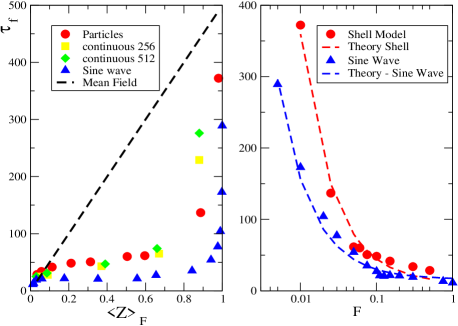
Fig.(2) shows the average fixation time $\tau_{f}$ for $s=0$ in the first two cases, at varying the intensity $F$ of advection. In the left panel, we plot the fixation times as a function of the time averaged reduced carrying capacity $\langle Z\rangle$, where $Z(t)=n(t)/N$ is the carrying capacity reduction, i.e. the ratio between the actual number of particles and the average number of particles $N$ observed in absence of the velocity field. Plotting vs. $\langle Z\rangle_{F}$ allows comparisons with the mean field prediction, $\tau_{f}=2N\langle Z\rangle_{F}/\mu$, valid for well mixed systems (black dashed line) 8 . For the shell model, we include simulations of the macroscopic equations (Population genetics in compressible flows) with different resolutions ($256$ and $512$ lattice sites on the unit interval), obtaining always similar results for $\tau_{f}$ vs. $\langle Z\rangle_{F}$.

In all cases, the presence of a spatially varying velocity field leads to a dramatic reduction of $\tau_{f}$, compared to the mean field theory. The fixation time drops abruptly as soon as $\langle Z\rangle<1$, even for very small $F$. Simulations suggest a singular limit of zero intensity ($F\sim 0$) of the velocity field (and consequently $\langle Z\rangle\rightarrow 1$ in Fig. 2), as we discuss later.

These observations can be understood by assuming that global fixation is determined by coalescence of allele boundaries like those shown in Fig. (1a). Although in the stochastic FKPP with $s=0$ the boundaries perform a random walk 8 , here they are also advected by the velocity field. In particular, the average position of one boundary $x$, neglecting diffusion and number fluctuations, will simply evolve according $\dot{x}=v(x,t)$. The fixation time is then determined by the time needed for the boundaries to reach the center of a sink and annihilate. Because periodic boundary conditions are imposed, the number of interfaces is necessarily even, so all of them annihilate pairwise. Upon expanding the velocity field around a sink position $x_{0}$, $v(x)=k(x_{0}-x)$, we find a fixation time $\sim k^{-1}$. Hence, we model the average time to fixation $\tau_{f}$ vs. the velocity field intensity as $\tau_{f}$=$\tau_{0}+ck^{-1}$, where $\tau_{0}$ represents the typical time to reach fixation at large strain rate $k$ and $c$ is an dimensionless constant of order unity. This phenomenological theory describes well the data of Fig. 2, right panel (dot-dashed lines), where in the turbulent case we take the forcing $F$ as a proxy for $k$ ($k=2\pi F$ for the sine wave and $k=\sqrt{\langle(\nabla v)^{2}\rangle}\propto F$ for turbulence).

We now study particles subject to a converging linear velocity, $v(x)=-kx$. When $k$ is large (and $\langle Z\rangle_{k}$ is small), the fixation time is comparable to the mean field prediction. However, as the forcing decreases, it becomes much larger than the mean field prediction (Fig. 3a, dashed line). In this regime, the fixation time probability distribution is bimodal (Fig. 3a, inset): roughly half of the realizations have a short fixation time (faster than mean field), while the other half maintain coexistence for an extended period. The space-time evolution of these configurations in Fig. 3b reveals that the two mutant species are demixed, one on the left and one on the right of the sink. Correspondingly, the average total heterozigosity $\langle H(t)\rangle$, defined as the probability of two random individuals to be of different type 8 , decays exponentially for very large $k$ (consistent with mean field theory 8 ), but tends to a constant, non-zero value when smaller values of $k$ are chosen (Fig 3c).

Figure 3: (a) Average fixation time $\tau_{f}$ in the presence of a linear converging flow $v=-kx$, as a function of the reduced carrying capacity $\langle Z\rangle_{k}$. Inset on left shows the distribution of fixation times in the case $k=0.075$ and $\langle Z\rangle_{k}\approx 0.38$, the right peak representing all realizations with fixation times $t>2000$. (b) Space-time plot of a realization with a very long fixation time. (c) Average heterozigosity as a function of time for different values of $k$.

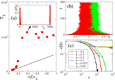
This remarkable behavior arises because of the different boundary conditions for the linear sink, such that the number of domain boundaries is no longer always even. Hence, the initial number of boundaries will be odd approximately half the time for random initial conditions, leading to the single surviving boundary as shown on the right of Fig. 3a. This configuration corresponds to a stable stationary solution of the deterministic version of Eqs Population genetics in compressible flows with $s=0$. We expect that this demixed solution, with $c_{A}(x)$ and $c_{B}(x)$ nonzero on opposite sides of the sink, should have a lifetime (inaccessible in numerical simulations) which grows exponentially with $N$ 9 ; 20 .

Figure 4: Coexistence of two species advected by a linear sink $k=0.075$, (left) species are neutral as in Fig. 3, (right) Red reproduces 30% faster. Notice the shift in the position of the boundary.

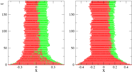
Finally, what happens for a selective advantage $s>0$? Fig. 4 shows a comparison between the neutral case of Fig. 3 and a simulation in which red particles reproduce $30\%$ faster ($s=0.3$). Even with such a large selective advantage, genetic interfaces are still present. In this case, we estimate the shift in the interface as $\delta x=k^{-1}2\sqrt{Ds}$, by equating the outward Fisher genetic wave velocity $v_{g}=2\sqrt{Ds}$ 1 with the inward advection velocity at distance $\delta x$ from the origin.

To conclude, we have introduced a new model which allows studies of how compressible advection affects Darwinian competition. A compressible flow leads to a radically new scenario, with the fixation time being largely determined by how species boundaries collapse into the sinks of the velocity field, rather than by diffusive annihilation. Our phenomenological theory suggests a significative effect even for very weak compressible fields. Compressible advection becomes irrelevant for the fixation time only when the time to drift into the sinks (of order $t\sim k^{-1}$) is much larger than the diffusion time (of order $L^{2}D^{-1}$, where $L$ is a typical linear size of the population). An obvious application of the model is the study of compressible flows in higher space dimensions, including flows relevant to biological oceanography of photosynthetic organisms near the water surface. Recent advances in experimental techniques could also lead to tests of the one dimensional results. Motility of bacteria has been studied in microstructures of diameter comparable or even smaller to that of the organisms mannik . In this setting, a compressible flow could be created by pumping liquid nutrient from the two ends of the tube and extracting it from the center via a semipermeable membrane. Another possibility could be to study floating microorganisms 15 ; rainey and make use of the compressible effects caused by the vertical component of a convecting velocity field 16 .

I SUPPLEMENTARY MATERIALS

In this note we present the technical derivations of the results in the Letter “Population Genetics in compressible flows” (“main text”). First, we describes the derivation of the macroscopic equations for the particle model introduced in the main text. Then, we describe details of the continuum simulations and of the shell model of turbulence. Finally, we discuss the relation between the model introduced in the main text and the simpler stochastic Fisher-Kolmogorov-Petrovsky-Piskounov (FKPP) equation (Eq. (1) of the main text).

II Macroscopic equations for the two species model

To derive the mean field version of the model discussed in the Letter. we consider first position-independent quantites $n_{A}$ and $n_{B}$ which represent the number of particles of species $A$ and $B$ respectively. This “zero-dimensional” limit corresponds to a single well mixed “deme” or island in a stepping stone model. The birth and death processes are characterized by the following transition rates:

$$W_{A}(+1,n_{A},n_{B}) = \mu n_{A}$$

$$W_{A}(-1,n_{A},n_{B}) = \tilde{\mu}n_{A}(n_{A}+n_{B})$$

$$W_{B}(+1,n_{A},n_{B}) = \mu n_{B}$$

$$W_{B}(-1,n_{A},n_{B}) = \tilde{\mu}n_{B}(n_{A}+n_{B})$$ (3)

where $W_{A}(+1,n_{A},n_{B})$ is the probability per unit time of population $A$ to increase its size by one unit when the total populations are $n_{A}$ and $n_{B}$, and similarly for $W_{A}(-1,n_{A},n_{B})$ and $W_{B}(\pm 1,n_{A},n_{B})$.

There exist several methods to derive macroscopic equations for particle models 9 ; risken ; 20 , most popular being the Van Kampen system size expansion and the Kramers-Moyal expansion. While the former is more rigorous when studying problems beyond the linear noise approximation, the latter is normally used because it leads to more transparent expressions. Moreover, it can be shown (see e.g. 9 , page 251) that at the order of the Fokker Planck equation the two methods are completely equivalent. The Kramers-Moyal method works as follows: consider a master equation, and call $W(\Delta n,n)$ the transition rate from $n$ particles to $n+\Delta n$ particles. When $n$ is typically large and $\Delta n$ relatively small ($\pm 1$ in the case of birth-death process considered here) a Taylor series expansion of the master equation in $\Delta n$ for the probability $P(n,t)$ of having $n$ particles at time $t$ is appropriate:

$$\partial_{t}P(n,t)=\sum\limits_{j=1}^{\infty}\frac{(-1)^{j}}{j!}\partial^{j}_{n}[\alpha_{j}(n)P(n,t)]$$ (4)

with

$$\alpha_{j}(n)=\int d\Delta n\ (\Delta n)^{j}W(\Delta n,n).$$ (5)

Truncating the Taylor expansion at the second order in $j$ leads to a Fokker-Planck equation.

It is straightforward to apply the above procedure to two species $A$ and $B$ and obtain the zero-dimensional Fokker-Planck equation for the joint probability distribution function $P(n_{A},n_{B},t)$. Substituting the expression of the transition rates of Eq. (II) into (4- 5) leads to:

$$\partial_{t}P(n_{A},n_{B},t)=-\partial_{A}[n_{A}(\mu-\tilde{\mu}n_{A}-\tilde{\mu}n_{B})P]-\partial_{B}[n_{B}(\mu-\tilde{\mu}n_{A}-\tilde{\mu}n_{B})P]+$$

$$+\frac{1}{2}\partial_{A}^{2}[n_{A}(\mu+\tilde{\mu}n_{A}+\tilde{\mu}n_{B})P]+\frac{1}{2}\partial_{B}^{2}[n_{B}(\mu+\tilde{\mu}n_{A}+\tilde{\mu}n_{B})P],$$ (6)

corresponding to the stochastic differential equations:

$$\frac{dn_{A}(t)}{dt}=n_{A}(\mu-\tilde{\mu}n_{A}-\tilde{\mu}n_{B})+\sqrt{n_{A}(\mu+\tilde{\mu}n_{A}+\tilde{\mu}n_{B})}\xi(t)$$

$$\frac{dn_{B}(t)}{dt}=n_{B}(\mu-\tilde{\mu}n_{A}-\tilde{\mu}n_{B})+\sqrt{n_{B}(\mu+\tilde{\mu}n_{A}+\tilde{\mu}n_{B})}\xi^{\prime}(t)$$ (7)

where $\xi(t)$ and $\xi^{\prime}(t)$ are delta-correlated Gaussian processes in time with unit amplitude, e.g. $\langle\xi(t_{1})\xi(t_{2})\rangle=\delta(t_{1}-t_{2})$ and are uncorrelated with each other, $\langle\xi(t_{1})\xi^{\prime}(t_{2})\rangle=0$ . For consistency we have to adopt the Ito prescription for interpreting the nonlinear noise term 9 .

From Eq. (II) we see that typical values of $n_{A}+n_{B}$ near the steady state are of order $N=\mu/\tilde{\mu}$. Upon defining the rescaled particle densities

$$c_{A}=\frac{n_{A}}{N}=\frac{\tilde{\mu}}{\mu}n_{A},\quad c_{B}=\frac{n_{B}}{N}=\frac{\tilde{\mu}}{\mu}n_{B},$$ (8)

we obtain

$$\frac{dc_{A}(t)}{dt}=\mu c_{A}(1-c_{A}-c_{B})+\sqrt{\frac{\mu c_{A}(1+c_{A}+c_{B})}{N}}\xi(t)$$

$$\frac{dc_{B}(t)}{dt}=\mu c_{B}(1-c_{A}-c_{B})+\sqrt{\frac{\mu c_{B}(1+c_{A}+c_{B})}{N}}\xi^{\prime}(t).$$ (9)

These coupled Langevin equations approximate well the master equation when $N=\mu/\tilde{\mu}$ is large. If $N$ is not large, the noise cannot be approximated by a Gaussian noise.

The model is generalized to include advection and diffusion in space as follows: Particles belonging to the two species advect and diffuse in space in a Lagrangian way, i.e. the position $x$ of a given particle evolves according to:

$$\frac{dx}{dt}=v(x)+\sqrt{2D}\zeta(t),$$ (10)

where $\zeta(t)$ is a unit amplitude Brownian noise source that implements diffusion with diffusion constant $D$. At each time step $dt$, a given particle duplicates with probability $\mu dt$ or annihilates due to competition with rate $\tilde{\mu}(\hat{n}_{A}+\hat{n}_{B})dt$, where $\hat{n}_{A,B}$ are now the number of particles of type $A,B$ in a region of size $\delta$ centered in the particle itself.

The macroscopic equations in the spatial case can be derived using arguments similar to the well mixed case. We assume that binary reactions can occur only when both particles are within a length $\delta$, and also take this as the size of our discretization volume. Although the total particle number in this region fluctuates, $\delta$ plays a role similar to an island spacing in a stepping stone model. We first write the discretized stochastic differential equation for the $n_{A}^{i}$ and $n_{B}^{i}$ , the number of particles in the $i^{th}$ cell of size $\delta$:

$$\frac{dn_{A}^{i}}{dt}=n_{A}^{i}(\mu-\tilde{\mu}n_{A}^{i}-\tilde{\mu}n_{B}^{i})+\mathrm{diffusion/advection}+\sqrt{n_{A}^{i}(\mu+\tilde{\mu}n_{A}^{i}+\tilde{\mu}n_{B}^{i})}\xi^{i}_{A}$$

$$\frac{dn_{B}^{i}}{dt}=n_{B}(\mu-\tilde{\mu}n_{A}^{i}-\tilde{\mu}n_{B}^{i})+\mathrm{diffusion/advection}+\sqrt{n_{B}^{i}(\mu+\tilde{\mu}n_{A}^{i}+\tilde{\mu}n_{B}^{i})}\xi^{i}_{B}$$ (11)

where the noise terms now obey $\langle\xi^{i}_{k}(t)\xi^{j}_{k^{\prime}}(t^{\prime})\rangle=\delta(t-t^{\prime})\delta_{j,j^{\prime}}\delta_{k,k^{\prime}}$.

Here, we assume the ration $N_{l}=\mu/\tilde{\mu}$ is adjusted to match the overall carrying capacity of the $i^{th}$ cell, and that $\delta$ is big enough to insure the local carrying capacity $N_{l}\gg 1$. When $N_{l}$ is sufficiently large, the diffusion and advection terms enter only in the deterministic part of our equations.

There are two possible choices for passing to the concentration equations:

1. Change variables to the integrated dimensionless concentration inside each cell: $c_{A,B}^{i}=n^{i}_{A,B}/N_{l}$.

2. Change variables to a normalized real concentration (number of particles per unit volume): $c_{A,B}^{i}=n^{i}_{A.B}/(N\delta^{d})$ in $d$ dimensions (we focus here on $d=1$).

In the first case, one is left with a discretized set of well defined Langevin equations, a natural generalization of the discrete stepping stone model with dimensionless species concentrations. The first procedure, after setting as before $N_{l}\tilde{\mu}=\mu$, results in:

$$\frac{dc_{A}^{i}}{dt} = \mu c_{A}^{i}(1-c_{A}^{i}-c_{B}^{i})+\mathrm{diffusion/advection}+\sqrt{\frac{\mu c_{A}^{i}(1+c_{A}^{i}+c_{B}^{i})}{N_{l}}}\xi^{i}_{A}$$

$$\frac{dc_{B}^{i}}{dt} = \mu c_{B}^{i}(1-c_{A}^{i}-c_{B}^{i})+\mathrm{diffusion/advection}+\sqrt{\frac{\mu c_{B}^{i}(1+c_{A}^{i}+c_{B}^{i})}{N_{l}}}\xi^{i}_{B}$$ (12)

which is a set of well defined stochastic differential equations, valid for a particular lattice spacing $\delta$.

The second procedure, however, leads to a more convenient passage to the continuum limit,

$$\frac{dc_{A}^{i}}{dt} = c_{A}^{i}[\mu-\tilde{\mu}N\delta(c_{A}^{i}-c_{B}^{i})]+\mathrm{diffusion/advection}+\sqrt{\frac{c_{A}^{i}[\mu+\tilde{\mu}N\delta(c_{A}^{i}+c_{B}^{i})]}{N\delta}}\xi^{i}_{A}$$

$$\frac{dc_{B}^{i}}{dt} = c_{B}^{i}[\mu-\tilde{\mu}N\delta(c_{A}^{i}-c_{B}^{i})]+\mathrm{diffusion/advection}+\sqrt{\frac{c_{B}^{i}[\mu+\tilde{\mu}N\delta(c_{A}^{i}+c_{B}^{i})]}{N\delta}}\xi^{i}_{B}$$ (13)

Starting with Eq.(II), a formal way to achieve the continuous limit is to set first $\tilde{\mu}N\delta=\mu$ by rescaling the densities. This choice corresponds to an average number of particles equal to $N_{l}$ in a cell in the absence of fluid flow when the total density $c_{A}+c_{B}$ is constant and equal to $1$. Then, we take the continuum limit at fixed $\mu$, leading to:

$$\partial_{t}c_{A}=-\partial_{x}(vc_{A})+D\partial^{2}_{x}c_{A}+\mu c_{A}(1-c_{A}-c_{B})+\sigma_{A}\xi$$ (14)

$$\partial_{t}c_{B}=-\partial_{x}(vc_{B})+D\partial^{2}_{x}c_{B}+\mu c_{B}(1-c_{A}-c_{B})+\sigma_{B}\xi^{\prime}$$ (15)

where now $<\xi(x,t)\xi^{\prime}(x^{\prime},t^{\prime})>=0$, $<\xi(x,t)\xi(x^{\prime},t^{\prime})>=\delta(t-t^{\prime})\delta(x-x^{\prime})$ and $<\xi^{\prime}(x,t)\xi^{\prime}(x^{\prime},t^{\prime})>=\delta(t-t^{\prime})\delta(x-x^{\prime})$ . We also defined $\sigma_{A}=\sqrt{\mu c_{A}(1+c_{A}+c_{B})/N}$ and $\sigma_{B}=\sqrt{\mu c_{B}(1+c_{A}+c_{B})/N}$. We have chosen units of length such that $L=1$. To return to dimensional units, simply let $1/N\rightarrow L/N$ in $\sigma_{A}$ and $\sigma_{B}$. To understand the connection with stepping stone models, it is helpful to note that $L/N=\delta/N_{l}$, so that the amplitude of the noise terms in Eqs. (14) and (15) can be written in a similar form as the “generic diffusion constant” discussed in Ref. 8 . Eqs. (14) and (15) correspond to the macroscopic equations presented in the Letter in absence of a selective advantage, $s=0$. The derivation of the non-neutral is a straightforward generalization in which the parameter $s$ controls the relative difference of the duplication rate of species $A$ with respect to that of species $B$. Mathematically, this correspondly to repeat the expansion but substituting to the first equation in (II) the more general expression:

$$W_{A}(+1,n_{A},n_{B})=\mu n_{A}\ \longrightarrow\ W_{A}(+1,n_{A},n_{B})=\mu(1+s)n_{A}$$ (16)

leading to the the expression of Eq. (2) in the main text.

The continuous limit of such reaction-diffusion-advection processes is only a concise summary of the stochastic dynamics; underlying this is always the space-discretized version (see Ref. 9 , page 314). One reason is that advection and diffusion terms can contribute significantly to the variance of the noise when the cells are small (9 , page 313); these terms can be neglected only if the equations will be discretized on a sufficiently coarse lattice. Moreover, the validity of the Kramers-Moyal (or Van Kampen) expansion relies on $N_{l}\gg 1$. Even in absence of a carrying capacity reduction due to compressible flows, the number of particles in a sufficiently small cell may not be particularly large. The macroscopic continuum equations will then be consistent with results from particle simulations only when there is a sufficiently large number of particles when we coarse-grain to scales small compared to the typical scales of the density gradients. This is the case for the parameter ranges considered in the main text.

III Continuous simulations and shell models

In addition to particle simulations, Eq.s (14-15) (i.e. Eqs. (2) in the main text) have been simulated numerically by using finite difference methods in space and the Euler-Cauchy method for time steps with a variety of velocity fields $v(x,t)$. The effect of number fluctuations (i.e. genetic drift) has been taken into account by using the method proposed by Doering et. al. doering : at each time step we compute the position-dependent quantities $\sigma_{A,B}=\mu c_{A,B}(1+c_{A}+c_{B})/N_{l}$. If $\sigma_{A,B}>0$ (i.e. if there is a non-zero number of particles of the appropriate type in the region of size $\delta$), then we add the noise term; otherwise we set the noise term equal to $0$. It has been shown by Doering et. al. that this numerical scheme converges, in a suitable norm, to the continuum limit. In our numerical simulations, we found excellent agreement between the results obtained by integrating eq.s (14-15) with this technique, compared to those obtained by particle methods, as will be discussed in details in a forthcoming paper.

Next we illustrate how we built the ”turbulent” velocity field $u(x,t)$ used in our high Reynolds number simulations. Although we focus primarily on one spatial dimension, our analysis of the statistical properties of $c(x,t)$ employs velocity fluctuations typical of three dimensional turbulent fluid mechanics. The statistical properties of our advecting velocity field $u(x,t)$ will be characterized by intermittency both in space and in time. To obtain a velocity field with generic space and time dynamics at high Reynolds number, we build up $u(x,t)$ by appealing to a simplified shell model of fluid turbulence biferale . Wavenumber space is divided into shells centered around $k_{n}=2^{n-1}k_{0}$, $n=1,2,...$. For each shell with characteristic wavenumber $k_{n}$, we describe turbulence by using the complex Fourier-like variable $u_{n}(t)$, satisfying the following equations of motion:

$$(\frac{d}{dt} + \nu k_{n}^{2})u_{n}=i[k_{n+1}u_{n+1}^{*}u_{n+2}-\Delta k_{n}u_{n-1}^{*}u_{n+1}$$ (17)

$$+ (1-\Delta)k_{n-1}u_{n-1}u_{n-2}]+f_{n}\ .$$

The model contains one free parameter, $\Delta$, and it conserves two quadratic invariants (when the force and the dissipation terms are absent) for all values of $\Delta$. The first is the total energy $\sum_{n}|u_{n}|^{2}$ and the second is $\sum_{n}(-1)^{n}k_{n}^{\alpha}|u_{n}|^{2}$, where $\alpha=\log_{2}(1-\Delta)$. We fix $\Delta=-0.4$, as this choice reproduces intermittency features of the real three dimensional Navier Stokes equation with surprising good accuracy biferale . Using $u_{n}$, we can build the real one dimensional velocity field $u(x,t)$ as

$$u(x,t)=F\sum_{n}[u_{n}(t)e^{ik_{n}x}+u^{*}_{n}(t)e^{-ik_{n}x}],$$ (18)

where the constant $F$ controls the strength of velocity fluctuations relative to other parameters in the model. In all numerical simulations we use a forcing function $f_{n}=[\epsilon(1+i)/u^{*}_{1}]\delta_{n,1}$, i.e. energy is supplied only to the largest scale corresponding to $n=1$, where $\epsilon$ is the injection rate of turbulent energy. With this choice, the power injected into the shell model is simply given by $1/2\sum_{n}[u^{*}_{n}f_{n}+u_{n}f^{*}_{n}]=\epsilon$ , i.e. it is constant in time. To solve Eqs. (14-15) and (17) we use a finite difference scheme with periodic boundary conditions in space.

IV Stochastic FKPP limit

In this section, we clarify the connection between the advection-free model described in the Letter and in Eqs. (14,15) and the stochastic FKPP (Fisher-Kolmogorov-Petrovsky-Piscounov) equation. To handle advecting flows, our model generalizates the FKPP equation by relaxing the constraint on the total density, $c_{A}(x,t)+c_{B}(x,t)=1$ for all values of $x$ and $t$, see Fig. (5).

Figure 5: Reaction plane. The dashed line is the steady state line with selective advantage $s=0$, $c_{A}+c_{B}=1$, where the model is equivalent to the stochastic FKPP equation . The trajectory is a zero-dimensional simulation of Eqs. (II) with $N=500$ and $\mu=1$.

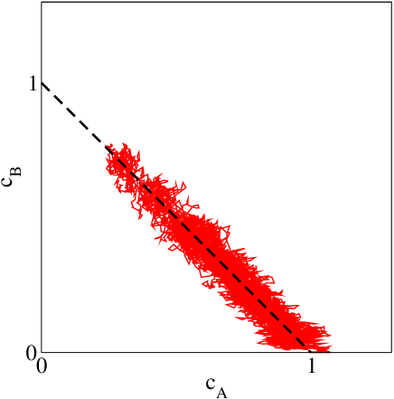
To understand this correspondence, it is helpful to change variables from the densities $c_{A}$, $c_{B}$ to the relative densities $f_{A,B}(x,t)=c_{A,B}(x,t)/c_{T}(x,t)$ where $c_{T}(x,t)=c_{A}(x,t)+c_{B}(x,t)$. Eqs. (14-15) now become:

$$\partial_{t}f_{A} = -[v-D\partial_{x}\log(c_{T})]\partial_{x}f_{A}+D\partial^{2}_{x}f_{A}+\sigma_{f_{A}}\xi$$

$$\partial_{t}f_{B} = -[v-D\partial_{x}\log(c_{T})]\partial_{x}f_{B}+D\partial^{2}_{x}f_{B}+\sigma_{f_{B}}\xi^{\prime}$$ (19)

where now the noise amplitudes are given by $\sigma^{2}_{f_{A},f_{B}}=\mu(1+c_{T})f_{A,B}(1-f_{A,B})/(Nc_{T})$ and by definition $f_{A}(x,t)+f_{B}(x,t)=1$.

Upon substituting $c_{T}=1$ and in absence of advection ($v=0$), each of the fractions evolves according to the stochastic FKPP equations for two neutral alleles.

A further issue is to understand if there is a limit in which the term $D\partial_{x}\log c_{T}$ can be neglected, so that one retrieves Eq. (IV) without having to impose any constraint. An estimate follows from studying the fluctuations of $c_{T}(x,t)=c_{A}(x,t)+c_{B}(x,t)$, which obeys a closed equation:

$$\partial_{t}c_{T}(x,t)=\mu c_{T}(1-c_{T})+D\partial^{2}_{x}c_{T}+\sqrt{\frac{\mu c_{T}(1+c_{T})}{N}}\xi(x,t)$$ (20)

where $\langle\xi(x,t)\xi(x^{\prime}t^{\prime})=\delta(x-x^{\prime})\delta(t-t^{\prime})$. By defining $\epsilon(x,t)=c_{T}(x,t)-1$ and assuming $\epsilon\ll 1$, we obtain a linear stochastic differential equation,

$$\partial_{t}\epsilon(x,t)=-\mu\epsilon+D\partial^{2}_{x}\epsilon+\sqrt{\frac{2\mu}{N}}\xi(x,t)$$ (21)

By means of a Fourier transform we can diagonalize the diffusion operator and find that the Fourier modes $\tilde{\epsilon}(k,t)=\int\ dx\exp(ikx)\epsilon(k,t)$ are independent Gaussian variables with zero mean and variance $\sigma^{2}(k)=2\mu/[N(\mu+Dk^{2})]$. It follows that

$$\langle|\epsilon(x,t)|^{2}\rangle\approx\frac{2\mu}{N}\int_{-\infty}^{+\infty}\frac{dk}{2\pi}\frac{1}{\mu+Dk^{2}}=\frac{1}{N}\sqrt{\frac{\mu}{D}}.$$ (22)

The fluctuations in $\epsilon(x,t)$ will be negligible when $N$ is large. In addition, it is interesting to study

$$\langle|D\partial_{x}\log c_{T}|^{2}\rangle\sim\langle|D\partial_{x}\epsilon|^{2}\rangle=\int_{-k_{max}}^{+k_{max}}\frac{dk}{2\pi N}\ \frac{2\mu D^{2}k^{2}}{\mu+Dk^{2}}$$ (23)

where we introduced a large $k$ cutoff (related to the discretization size, $|k_{max}|\sim\delta^{-1}$) in the above integral to avoid an ultraviolet divergence. With this premise, the above integral is small if $D$ is small, suggesting that the logarithmic terms in Eqs. (IV) can be neglected in this limit.

References

- (1) R. A. Fisher, Ann. Eugenics 7, 353-369 (1937).
- (2) A. Kolmogorov, N. Petrovsky, and N. Piscounov, Moscow Univ. Math. Bull. 1, 1-25 (1937).
- (3) W. van Saarloos, Phys. Rep. 386, 29-222 (2003).
- (4) M. Kimura and G. H. Weiss, Genetics 49, 561-576 (1964); J. F. Crow and M. Kimura An Introduction to Population Genetics, Blackburn Press, Caldwell, NJ (2009).
- (5) O. Hallatschek and K. Korolev, Phys. Rev. Lett. 103, 108103 (2009), and references therein.
- (6) For a recent review, see K. Korolev et al. Rev. Mod. Phys. 820, 1691-1718 (2010).
- (7) C. Gardiner Handbook of Stochastic Methods: for Physics, Chemistry and the Natural Sciences, Springer Series in Synergetics (2004).
- (8) B. A. Whitton and M. Potts The Ecology of Cyanobacteria: Their Diversity in Time and Space eds. Kluwer, Dordrecht, Netherlands (2000).
- (9) T .Tel et al., Physics Reports 413, 91–196 (2005).
- (10) F. D’Ovidio et al., Proc. Natl. Acad. Sci. 107, 18366-18370 (2010).
- (11) W. J. McKiver and Z. Neufeld, Phys. Rev. E 79, 061902 1-8 (2009).
- (12) J. Bec, Phys. Fluids 15, L81-L84 (2003).
- (13) A. P. Martin, Progr. Ocean. 57, 125-174 (2003).
- (14) J. R. Cressman et al., Europhys. Lett. 66, 219-225 (2004); G. Boffetta et al., Phys. Rev. Lett. 93, 134501 (2004).
- (15) R. Benzi, D. R. Nelson Physica D 238 2003-2015 (2009).
- (16) P. Perlekar et al., Phys. Rev. Lett. 105, 144501 (2010).
- (17) M. H. Jensen et al., Phys. Rev. A 43, 798-805 (1991) ; T. Bohr et al., Dynamical Systems Approach to Turbulence Cambridge University Press, Cambridge (1998).
- (18) Supplementary Material are available online.
- (19) N. G. van Kampen Stochastic Processes in Physics and Chemistry, Elsevier, Amsterdam (2007).
- (20) M. O. Vlad et al., Phys. Rev. E 65, 061110 (2002); M. O. Vlad et al., Proc. Natl. Acad. Sci. 13, 10249-10253 (2004).
- (21) J. Männik et al. Proc. Natl. Acad. Sci. 35, 14861-14866 (2009).
- (22) P. B. Raney and M. Travisano Nature 294, 69-72 (1998).
- (23) Risken H (1996) The Fokker-Planck Equation: Methods of Solution and Applications, Springer-Verlag, Berlin.
- (24) Biferale L (2003) Annu. Rev. Fluid Mech. 35, 441.
- (25) Doering CR, Sargsyan KV, Smereka P (2005) Physics Letters A 344: 149D155; see also Doering CR, Mueller C and Smereka P (2003) Physica A 325: 243-259.