Thermodynamics of the one-dimensional frustrated Heisenberg ferromagnet with arbitrary spin

Abstract

The thermodynamic quantities (spin-spin correlation functions $\langle{\bf S}_{0}{\bf S}_{n}\rangle$, correlation length $\xi$, spin susceptibility $\chi$, and specific heat $C_{V}$) of the frustrated one-dimensional $J_{1}$-$J_{2}$ Heisenberg ferromagnet with arbitrary spin quantum number $S$ below the quantum critical point, i.e. for $J_{2}<|J_{1}|/4$, are calculated using a rotation-invariant Green-function formalism and full diagonalization as well as a finite-temperature Lanczos technique for finite chains of up to $N=18$ sites. The low-temperature behavior of the susceptibility $\chi$ and the correlation length $\xi$ is well described by $\chi=\frac{2}{3}S^{4}\left(|J_{1}|-4J_{2}\right)T^{-2}+AS^{5/2}\left(|J_{1}|-4J_{2}\right)^{1/2}T^{-3/2}$ and $\xi=S^{2}\left(|J_{1}|-4J_{2}\right)T^{-1}+BS^{1/2}\left(|J_{1}|-4J_{2}\right)^{1/2}T^{-1/2}$ with $A\approx 1.1\ldots 1.2$ and $B\approx 0.84\ldots 0.89$. The vanishing of the factors in front of the temperature at $J_{2}=|J_{1}|/4$ indicates a change of the critical behavior of $\chi$ and $\xi$ at $T\to 0$. The specific heat may exhibit an additional frustration-induced low-temperature maximum when approaching the quantum critical point. This maximum appears for $S=1/2$ and $S=1$, but was not found for $S>1$.

I Introduction

The one-dimensional (1D) Heisenberg model with ferromagnetic nearest-neighbor (NN) exchange $J_{1}<0$ and frustrating antiferromagnetic next nearest-neighbor (NN) exchange $J_{2}\geq 0$ has recently attracted much attention, see, e.g., Refs. bader79, ; chubukov, ; honecker, ; krivnov07, ; krivnov08, ; hiki, ; haertel08, ; zinke09, ; lauchli09, ; sirker2010, ; haertel11, ; nishimoto, . This model may serve as the minimal model to describe the physical properties of edge-shared chain cuprates, e.g. Ca₂Y₂Cu₅O₁₀, Li₂ZrCuO₄, and Li₂CuO₂.Kudo05 ; drechsQneu ; malek ; nishimoto On the other hand, several materials considered as 1D ferromagnets, such as TMCuC[(CH₃)₄NCuCl₃],TMCuC , CsNiF₃,steiner Ni(4-cyanopyridine)₂Cl₂landee or deposited Co chainsCo_chains might have also a weak frustrating NNN exchange $J_{2}<-J_{1}/4$. Moreover, recent investigations suggest that Li₂CuO₂ as well as Ca₂Y₂Cu₅O₁₀ are quasi-1D spin systems with a dominant ferromagnetic $J_{1}$ and weak frustrating antiferromagnetic $J_{2}$ so that the inchain spin-spin correlations are predominantly ferromagnetic.Kudo05 ; malek ; nishimoto

The corresponding Hamiltonian of the 1D $J_{1}$-$J_{2}$ Heisenberg model considered in this paper is given by

$$H=\sum_{i}\left(J_{1}{\bf S}_{i}{\bf S}_{i+1}+J_{2}{\bf S}_{i}{\bf S}_{i+2}\right),$$ (1)

where $i$ runs over all lattice sites and ${\bf S}_{i}^{2}=S(S+1)$. We set $J_{1}=-1$ and consider $J_{2}\geq 0$. Although some of the above mentioned materials, namely CsNiF₃,steiner Ni(4-cyanopyridine)₂Cl₂landee or deposited Co chainsCo_chains , represent 1D ferromagnets with spin quantum number $S>1/2$, so far the focus of recent theoretical studies has been on the $S=1/2$ case. Since Haldane’s famous paperhaldane we know that in 1D Heisenberg systems the spin quantum number may play a crucial role. Recently it has been found that the frustrated model (1) in the extreme quantum case $S=1/2$ may exhibit a different behavior near the quantum critical point than the model for $S>1/2$.krivnov07 Moreover, in Ref. ihle_new, it has been found that for the unfrustrated 1D quantum ferromagnets a characteristic field-induced low-temperature maximum in the specific heat exists only for the small spin quantum numbers $S=1/2$ and $S=1$, see also Refs. haertel11, ; magfeld, ; antsyg, .

In the present paper we discuss the thermodynamics of the model (1) for arbitrary spin quantum number $S$ and focus on the parameter regime $J_{2}<|J_{1}|/4$, where the ferromagnetic ground state is realized. It has been recently demonstrated for low-dimensional frustrated ferromagnets,haertel08 ; haertel10 ; dmitriev_clas ; haertel11 that the frustrating $J_{2}$ may influence the thermodynamics substantially. In the 1D system a change in the low-temperature behavior of the susceptibility and the correlation length as well as an additional low-temperature maximum in the specific heat have been found when approaching the zero-temperature critical point at $J_{2}=|J_{1}|/4$ from the ferromagnetic side.haertel08 In particular, a different critical behavior of the susceptibility and the correlation length has been found for $J_{2}<|J_{1}|/4$ and at $J_{2}=|J_{1}|/4$.haertel08 ; dmitriev_clas

As in our previous papers on frustrated spin-$1/2$ ferromagnets,haertel08 ; haertel10 ; haertel11 we use a second-order Green-function techniquekondo to study the influence of the spin quantum number $S$ on the thermodynamic properties of the model (1). This technique has been applied successfully to several low-dimensional quantum spin systems. rgm_new ; magfeld ; antsyg ; ihle_new ; junger05 ; junger09 ; haertel08 ; haertel10 ; haertel11 ; kondo ; SSI94

To extend our Green’s function theoryhaertel08 to $S>1/2$, we follow Ref. junger09, , where the Green’s function technique was applied to a ferro- and antiferromagnetic layered square lattice with arbitrary $S$. We complement the Green’s function results by full exact diagonalization (ED) and finite-temperature Lanczos (FTL) technique data for finite systems of up to $N=18$ lattice sites.

II Full diagonalization and finite-temperature Lanczos technique for finite lattices

Using Schulenburg’s spinpackspinpack and exploiting the lattice symmetries and the fact that $S^{z}=\sum_{i}S_{i}^{z}$ commutes with $H$ we are able to calculate the exact thermodynamics for periodic chains of up to $N=14$ spins for spin quantum number $S=1$. For $N=8$ sites we found the exact thermodynamics up to $S=2$. Clearly, the full ED of finite systems for $S>1/2$ is less efficient as for $S=1/2$, since the accessible system size $N$ decreases with increasing of $S$.

In addition to the full ED we have also applied a FTL technique, see e.g. Refs. prelov, ; schnack, . This method allows an accurate calculation of thermodynamic quantities down to low temperatures for $S=1$ up to $N=18$.

III Spin-rotation-invariant Green-function theory

To study the thermodynamics of the model (1) for arbitrary $N$ we use the spin-rotation-invariant Green-function method (RGM). haertel08 ; kondo ; rgm_new ; haertel10 ; junger09 ; SSI94 The relevant thermodynamic quantities can be determined by calculating the two-time commutator Green function elk $\langle\langle S_{q}^{+};S_{-q}^{-}\rangle\rangle_{\omega}$, which is related to the transverse spin susceptibility by $\chi_{q}^{+-}\left(\omega\right)=-\langle\langle S_{q}^{+};S_{-q}^{-}\rangle\rangle_{\omega}$ . Using the equations of motion up to the second step and supposing rotational symmetry with $\langle S_{i}^{z}\rangle=0$, we obtain $\omega^{2}\langle\langle S_{q}^{+};S_{-q}^{-}\rangle\rangle_{\omega}=M_{q}+\langle\langle-\ddot{S}_{q}^{+};S_{-q}^{-}\rangle\rangle_{\omega}$ with $M_{q}=\langle\left[\left[S_{q}^{+},H\right],S_{-q}^{-}\right]\rangle$ and $-\ddot{S}_{q}^{+}=\left[\left[S_{q}^{+},H\right],H\right]$. For the moment $M_{q}$ the exact expression

$$M_{q}=-4\sum_{n=1,2}J_{n}C_{n}\left(1-\cos nq\right)$$ (2)

holds, where $C_{n}=\langle S_{0}^{+}S_{n}^{-}\rangle=2\langle S_{0}^{z}S_{n}^{z}\rangle$. The second derivative $-\ddot{S}_{q}^{+}$ is approximated in the spirit of Refs. SSI94, ; kondo, ; rgm_new, ; magfeld, ; antsyg, ; haertel10, ; ihle_new, ; junger05, ; junger09, , i.e., in $-\ddot{S}_{i}^{+}$ we use the decoupling $S_{i}^{+}S_{j}^{+}S_{k}^{-}=\alpha\langle S_{j}^{+}S_{k}^{-}\rangle S_{i}^{+}+\alpha\langle S_{i}^{+}S_{k}^{-}\rangle S_{j}^{+}$, and $S_{i}^{+}S_{j}^{-}S_{j}^{+}=\langle S_{j}^{-}S_{j}^{+}\rangle S_{i}^{+}+\lambda\langle S_{i}^{+}S_{j}^{-}\rangle S_{j}^{+}$ for products with two coinciding sites which occur for $S\geq 1$.ihle_new ; junger05 ; junger09 ; SSI94 Note that for $J_{2}<-J_{1}/4$, where the ground-state is ferromagnetic, the vertex parameters $\alpha$ and $\lambda$ can be assumed in a good approximation to be independent of the range of the associated spin correlators, cf. Ref. haertel08, . Then we obtain $-\ddot{S}_{q}^{+}=\omega_{q}^{2}S_{q}^{+}$ and

$$\chi_{q}^{+-}\left(\omega\right)=-\langle\langle S_{q}^{+};S_{-q}^{-}\rangle\rangle_{\omega}=\frac{M_{q}}{\omega_{q}^{2}-\omega^{2}},$$ (3)

with

$$\omega_{q}^{2}=\hskip-8.53581pt\sum_{n,m(=1,2)}\hskip-8.53581ptJ_{n}J_{m}\left(1-\cos nq\right)\left[K_{n,m}+4\alpha C_{n}\left(1-\cos mq\right)\right],$$ (4)

where $K_{n,n}=\frac{4}{3}S\left(S+1\right)+2\lambda C_{n}+2\alpha\left(C_{2n}-3C_{n}\right)$, $K_{1,2}=2\alpha\left(C_{3}-C_{1}\right)$, and $K_{2,1}=K_{1,2}+4\alpha\left(C_{1}-C_{2}\right)$. From the Green function (3) the correlation functions $C_{n}=\frac{1}{N}\sum_{q}C_{q}e^{iqn}$ are determined by the spectral theorem,elk

$$C_{q}=\langle S_{q}^{+}S_{-q}^{-}\rangle=\frac{M_{q}}{2\omega_{q}}\left[1+2n\left(\omega_{q}\right)\right],$$ (5)

where $n(\omega_{q})=\left(e^{\omega_{q}/T}-1\right)^{-1}$ is the Bose function. Using the operator identity ${\bf S}_{i}^{2}=S_{i}^{+}S_{i}^{-}-S_{i}^{z}+\left(S_{i}^{z}\right)^{2}$, we get the sum rule $C_{0}=\frac{1}{N}\sum_{q}C_{q}=\frac{2}{3}S\left(S+1\right)$. Following Ref. junger09, , as an additional equation to determine the vertex parameters we consider the ratio

$$r(T)=\frac{\lambda(T)-\lambda(\infty)}{\alpha(T)-\alpha(\infty)}=r(0)$$ (6)

as temperature independent, where $\lambda(\infty)=1-\frac{3}{4S(S+1)}$ and $\alpha(\infty)=1$, see Ref. junger05, . The uniform static spin susceptibility $\chi=\lim_{q\to 0}\chi_{q}$, where $\chi_{q}=\chi_{q}\left(\omega=0\right)$ and $\chi_{q}\left(\omega\right)=\frac{1}{2}\chi_{q}^{+-}\left(\omega\right)$, is given by

$$\chi=-\frac{2}{\Delta}\sum_{n=1,2}n^{2}J_{n}C_{n}\,;\quad\Delta=\hskip-2.84526pt\sum_{n,m(=1,2)}\hskip-2.84526ptn^{2}J_{n}J_{m}K_{n,m}.$$ (7)

The correlation length $\xi$ for a ferromagnet can be calculated from the expansion of the static spin susceptibility around $q=0$ (see, e.g., Refs. kondo, and ihle_new, ), $\chi_{q}=\chi/\left(1+\xi^{2}q^{2}\right)$. The ferromagnetic long-range order, occurring in the 1D model at zero temperature only, is related to the condensation term $C$ (see Ref. kondo, ) via $C_{n}\left(0\right)=\frac{1}{N}\sum_{q(\neq 0)}\left(M_{q}/2\omega_{q}\right)e^{iqn}+C$. Equating this expression to the exact result $C_{n}\left(0\right)=\frac{2}{3}S\delta_{n,0}+\frac{2}{3}S^{2}$ leads to $C(0)=\frac{2}{3}S^{2}$ and $M_{q}(0)/2\omega_{q}(0)=\frac{2}{3}S$.junger09 This requires $\alpha(0)=\frac{3}{2}$ and $K_{n,m}(0)=0$ [cf. Eqs. (2) and (4)] which leads to $\lambda(0)=2-\frac{1}{S}$. The parameter $\Delta$ in Eq. (7) is zero at $T=0$, i.e., $\chi$ diverges as $T\to 0$ according to the ferromagnetic phase transition. Moreover, using these results we find at zero temperature $\omega_{q}=2\rho_{s}{q}^{2}$ ($|{q}|\ll 1$), $\rho_{s}=\frac{S}{2}(|J_{1}|-4J_{2})$, where $\rho_{s}$ is the spin stiffness.

Since we will compare the RGM data with ED data for finite lattices, see Sec. IV, we have to adopt the RGM to finite $N$. In this case the quantity $C$ is not related to the magnetisation and stays nonzero in the whole temperature region. In Ref. junger05, it was shown that $C=2T\chi/N$.

Finally, to solve the equation of motion and to evaluate the thermodynamic quantities we have to determine the correlators $C_{l}$ ($l=1,\ldots,4$) and the vertex parameters $\alpha$ and $\lambda$ (for finite systems, also $C$) as the numerical solution of a coupled system of six (seven) non-linear algebraic self-consistency equations: $C_{l}$ according to Eq. (5) including the sum rule $C_{0}=\frac{1}{2}$, and the ratio Eq. (6). To find the numerical solution of the RGM equations for $T>0$, we start at high temperatures and decrease $T$ in small steps. Below a certain (low) temperature $T_{0}(J_{2},S)$ no solutions of the RGM equations (except at $T=0$) could be found, since the quantity $\Delta(T,J_{2},S)$ in Eq. (7) becomes exponentially small which leads to numerical uncertainties. We find that $T_{0}(J_{2},S)/S(S+1)$ is of the order of $10^{-3}$ for all values of $J_{2}$ and $S$ considered here. Moreover, we find that the RGM solution at very low temperatures becomes less trustworthy for $J_{2}$ approaching the quantum critical point $J_{2}=|J_{1}|/4$, cf. also Refs. haertel08, and haertel11, . Therefore, below we will present RGM results for $J_{2}\leq 0.22|J_{1}|$ only.

Figure 1: Spin-spin correlation functions $\langle{\bf S}_{0}{\bf S}_{1}\rangle/S^{2}$ (NN), $\langle{\bf S}_{0}{\bf S}_{2}\rangle/S^{2}$ (NNN), and $\langle{\bf S}_{0}{\bf S}_{10}\rangle/S^{2}$ obtained by the RGM for spin quantum numbers $S=1$ (solid), $3/2$ (long-dashed), and $S=2$ (short-dashed) and frustration parameters $J_{2}=0$ (black), $0.1$ (red), and $0.2$ (blue).

IV Results

Motivated by the high-temperature behavior of the physical quantitiesdomb_green ; OHZ06 we use as the renormalized temperature scale $t=T/S(S+1)$, since for large temperatures physical quantities exhibit $t$-dependence which is independent of $S$.

IV.1 Spin-spin correlation functions

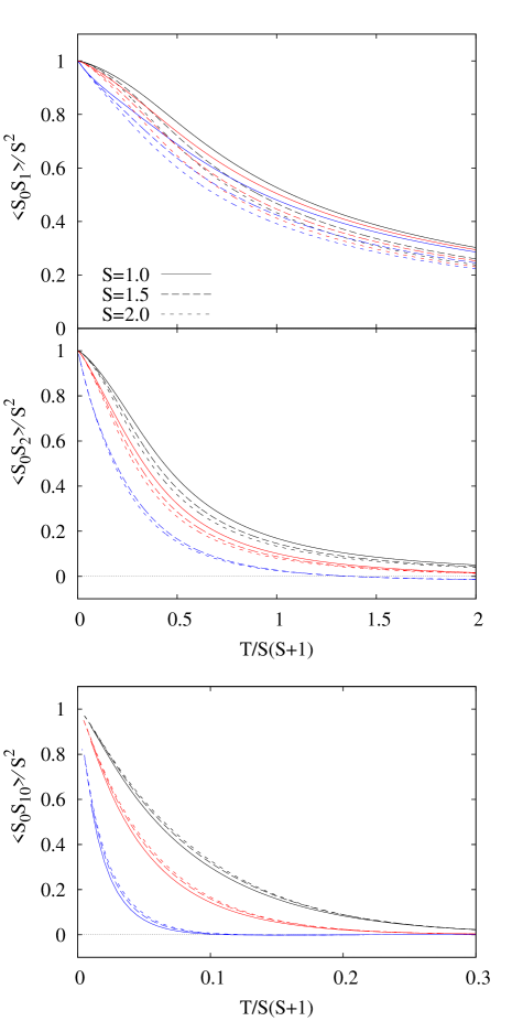
Let us first consider the spin-spin correlation functions $\langle{\bf S}_{0}{\bf S}_{n}\rangle$ depicted in Fig. 1 for NN, NNN and tenth-nearest neighbors. Analogously to the frustrated $S=1/2$ chain,haertel08 with increasing frustration the correlation functions decrease more rapidly. Obviously the spin quantum number $S$ has only a small influence on the correlation functions as functions of $t$. Interestingly, an increase of $S$ yields a slight weakening of the short-range spin-spin correlation at fixed $t>0$ (see upper and middle panels in Fig. 1), but an enhancement of larger-distant correlations (see lower panel in Fig. 1). Moreover, the NNN correlation function for $J_{2}=0.2$ becomes negative at $t=t_{0}\approx 1.35,1.37,1.38$ for $S=1,3/2,2$, respectively. (Note that for $S=1/2$ the corresponding temperature is $t_{0}\approx 1.27$.haertel08 )

Figure 2: Susceptibility $\chi$ for spin quantum number $S=1$ and frustration parameters $J_{2}=0$ (black), $0.1$ (red), $0.2$ (blue), and $0.22$ (violet) [solid lines: RGM for $N\to\infty$, dashed lines: RGM for $N=12$, symbols: ED for $N=12$]. Inset: Susceptibility $\chi$ for $J_{2}=0.1$ and $S=1/2$, $1$, $3/2$, and $2$ (from bottom to top). The data for $S=1/2$ are taken from Ref. haertel08, .

Figure 3: Correlation length $\xi$ for spin quantum number $S=1$ and frustration parameters $J_{2}=0$ (black), $0.1$ (red), $0.2$ (blue), and $0.22$ (violet). Inset: Correlation length $\xi$ for $J_{2}=0.1$ and $S=1/2$, $1$, $3/2$, and $2$ (from bottom to top). The data for $S=1/2$ are taken from Ref. haertel08, .

IV.2 Susceptibility and correlation length

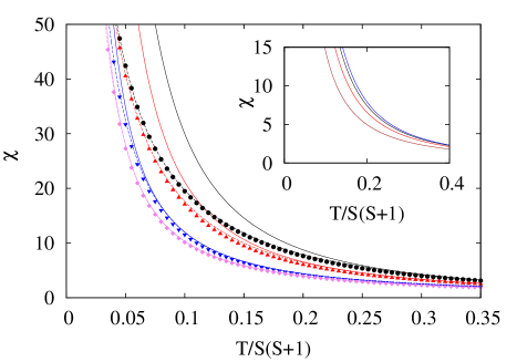
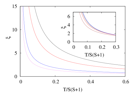
The behavior of the correlation functions is reflected in the susceptibility $\chi$ and the correlation length $\xi$ shown in Figs. 2 and 3. We illustrate the influence of frustration for a fixed spin quantum number $S=1$, whereas in the insets we show the influence of $S$ for a fixed frustration parameter $J_{2}=0.1$. Since the ground state is ferromagnetic, both quantities diverge at $T=0$. With increasing of frustration the rapid increase in $\chi$ and $\xi$ is shifted to lower temperatures. The comparison of RGM and ED results for finite chains of $N=12$ presented in Fig. 2 demonstrates a very good agreement of the susceptibility data obtained by both methods. It can also be seen that the renormalized temperature $t$, where finite-size effects become relevant, is shifted to lower values of $t$ with increasing frustration (in Fig. 2 the curves for $N=12$ and $N\to\infty$ for $J_{2}=0.2$ and $J_{2}=0.22$ almost coincide). The curves shown in the insets again illustrate that the influence of the spin quantum number is small; only for $S=1/2$ the curves are noticeably separated from the bundle of curves for $S>1/2$. Moreover, it is evident that $\chi$ and $\xi$ at fixed $t$ and $J_{2}$ increase with growing $S$.

Figure 4: RGM results for $\frac{3}{2}\chi T^{2}/S^{4}$ (upper panel) and $\xi T/S^{2}$ (lower panel) versus $\sqrt{T}$ for spin quantum numbers $S=1$ (solid), $3/2$ (long-dashed), and $S=2$ (short-dashed) and frustration parameters $J_{2}=0$ (black), $0.1$ (red), and $0.2$ (blue).

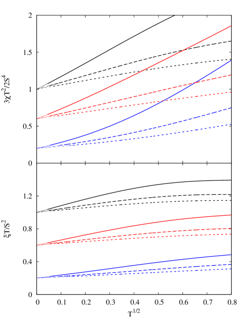
Next we consider the critical behavior of $\chi$ and $\xi$ for $T\to 0$ by analyzing the RGM data at low temperatures. From Ref. SSI94, it is known that within the RGM the low-temperature behavior of $\chi$ and $\xi$ of the unfrustrated ferromagnet ($J_{2}=0$) is given by $\lim_{T\to 0}\chi T^{2}=2S^{4}|J_{1}|/3$ and $\lim_{T\to 0}\xi T=S^{2}|J_{1}|$. These results agree with those obtained by modified spin-wave theory.takahashi ; yamada2 Moreover, for $S=1/2$ they coincide with the exact Bethe-ansatz analysis.yamada1 ; yamada2 (Note that $\chi$ defined in Refs. takahashi, and yamada1, is larger by a factor of four than $\chi$ given by Eq. (7).) Including higher-order terms in $T$ for 1D Heisenberg ferromagnets the low-temperature behavior of the susceptibility and the correlation length reads $\chi T^{2}=y_{0}+y_{1}\sqrt{T}+y_{2}T+{\cal O}(T^{3/2})$ and $\xi T=x_{0}+x_{1}\sqrt{T}+x_{2}T+{\cal O}(T^{3/2})$, see, e.g., Refs. yamada1, ; yamada2, ; takahashi, ; haertel08, . The dependence of $\chi T^{2}$ and $\xi T$ on $T^{1/2}$ is shown in Fig. 4 for various values of $S$ and $J_{2}$. The validity of linear relations $\chi T^{2}\propto T^{1/2}$ and $\xi T\propto T^{1/2}$ at low temperatures is clearly seen. To determine the parameters $y_{0}$, $y_{1}$, $y_{2}$, $x_{0}$, $x_{1}$, and $x_{2}$, we follow the lines of Ref. haertel08, and fit the RGM results for $\chi$ and $\xi$ using the relations given above. For the fits we use low-temperature data points between $T_{0}$ and $T_{0}+T_{cut}$, where $T_{0}$ is the lowest temperature for which solutions of the RGM equations can be found, see Sec. III. For $T_{cut}$ we chose $T_{cut}=0.005$, cf. Ref. haertel08, . By analyzing data for $J_{2}=0$ and $S=1$, $3/2$, $2$ and $5$ we have numerically confirmed the relations $y_{0}=2S^{4}/3$ and $x_{0}=S^{2}$ with an accuracy of at least three digits. For the next-to-leading coefficients we adopt the relations $y_{1}/S^{4}=\alpha_{0}S^{\alpha_{1}}$ and $x_{1}/S^{2}=\beta_{0}S^{\beta_{1}}$ found by modified spin-wave theory for the unfrustrated model.takahashi ; yamada2 We find $\alpha_{0}=1.106$, $\alpha_{1}=-1.497$, $\beta_{0}=0.834$, and $\beta_{1}=-1.495$, which is in good agreement with the results of Refs. takahashi, and yamada2, , where $\alpha_{0}=0.824$, $\alpha_{1}=-1.5$, $\beta_{0}=0.412$, and $\beta_{1}=-1.5$ were reported.

Now we determine the parameters $y_{0}$, $y_{1}$, $y_{2}$, $x_{0}$, $x_{1}$, and $x_{2}$ for finite frustration $J_{2}>0$. The results for the leading coefficients $y_{0}$ and $x_{0}$ are shown in the insets of Fig. 5. Both coefficients $y_{0}$ and $x_{0}$ obey with high precision the linear relations $y_{0}/S^{4}=\frac{2}{3}\left(|J_{1}|-4J_{2}\right)\,$ and $x_{0}/S^{2}=|J_{1}|-4J_{2}$, i.e., the leading coefficients decrease with growing frustration and vanish finally at the quantum critical point $J^{c}_{2}=|J_{1}|/4$, thus indicating a change of the critical exponent of $\chi$ and $\xi$ at $J^{c}_{2}$. This linear decrease of $y_{0}$ and $x_{0}$ found by fitting the low-temperature behavior of $\chi$ and $\xi$ is the same as that obtained analytically for the zero-temperature spin stiffness $\rho_{s}$, see Sec. III. This correspondence between the spin stiffness and the divergence of the susceptibility and the correlation length is in accordance with general argumentsivanov ; kopietz91 concerning the low-temperature physics of low-dimensional Heisenberg ferromagnets. Moreover, these linear relations agree with the findings for $S=1/2$ (Ref. haertel08, ) and $S\to\infty$ (Ref. dmitriev_clas, ).

Figure 5: Next-to-leading coefficients $y_{1}/S^{5/2}$ (upper panel) and $x_{1}/S^{1/2}$ (lower panel) in dependence on $J_{2}$ obtained by fitting the low-temperature data of $\chi$ and $\xi$ (see main text). The symbols represent the data points for $S=1/2$, $1$, $3/2$, $2$, and $S=5$, and the lines of the same color show the corresponding fit curves of these points using the fit function $f(J_{2})=a\sqrt{1-bJ_{2}}$. The thick black solid line shows the quadratic fit for $S=1/2$ without the data point at $J_{2}=0.22$ as used in Ref. haertel08, .
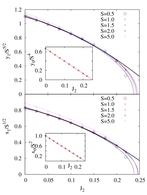
Insets: Leading coefficients $y_{0}$ (upper panel) and $x_{0}$ (lower panel) in dependence on $J_{2}$ obtained by fitting the low-temperature data of $\chi$ and $\xi$ (see main text). The values for $y_{0}/S^{4}$ as well as for $x_{0}/S^{2}$ practically coincide for $S=1/2$, $1$, $3/2$, $2$, and $S=5$ used to determine $y_{0}/S^{4}$ and $x_{0}/S^{2}$.

Next we determine the coefficients $y_{1}$ and $x_{1}$ as functions of $J_{2}$ again using the fit of the RGM data for $S=1$, $3/2$, $2$ and $5$ described above. Moreover, we reanalyze our data for $S=1/2$ from Ref. haertel08, . Using an improved computer code we are able to add $S=1/2$ data for $J_{2}=0.22$ not given in Ref. haertel08, . Similar as for $y_{0}/S^{4}$ and $x_{0}/S^{2}$, the data for $y_{1}$ and $x_{1}$ shown in Fig. 5 yield evidence for a universal $J_{2}$ dependence of $y_{1}/S^{5/2}$ and $x_{1}/S^{1/2}$. However, the coincidence of the data points is less pronounced (in particular for $S=5$) than for $y_{0}$ and $x_{0}$. The dependence of $y_{1}/S^{5/2}$ and $x_{1}/S^{1/2}$ on $J_{2}$ is clearly not linear. As suggested by the behavior of $y_{1}/S^{5/2}$ and $x_{1}/S^{1/2}$ at larger $J_{2}$ we chose $f(J_{2})=a\sqrt{1-bJ_{2}}$ to fit the data points presented in Fig. 5. These fits suggest, that $y_{1}$ and $x_{1}$ also vanish approaching the quantum critical point. Indeed, we find for the fit parameter $b\approx 4.08$ for most of the fits; only for $S=1/2$ we have $b\approx 4.20$. For comparison, we also show the previous quadratic fit for $S=1/2$ of Ref. haertel08, , where the data point at $J_{2}=0.22$ was not included. It is obvious that the square-root fit is more reasonable than the qadratic fit (which leads to a finite $y_{1}$ and $x_{1}$ at $J_{2}=|J_{1}|/4$). Moreover, a square-root dependence of $y_{1}$ and $x_{1}$ on the exchange couplings is also suggested by modified spin-wave theory.takahashi ; yamada2 ; sirker2011 Based on the results for $y_{0}$, $y_{1}$, $x_{0}$, and $x_{1}$ discussed above we finally argue that the low-temperature behavior of the susceptibility and the correlation length for $J_{2}<|J_{1}|/4$ is well described by

$$\chi T^{2}=\frac{2}{3}S^{4}\left(|J_{1}|-4J_{2}\right)+AS^{5/2}\sqrt{\left(|J_{1}|-4J_{2}\right)}\sqrt{T}$$ (8)

and

$$\xi T=S^{2}\left(|J_{1}|-4J_{2}\right)+BS^{1/2}\sqrt{\left(|J_{1}|-4J_{2}\right)}\sqrt{T}$$ (9)

with $A\approx 1.1$ ($A\approx 1.2$) and $B\approx 0.84$ ($B\approx 0.89$) for $S=1/2$, $1$, $3/2$, and $2$ ($S=5$). Therefore, we conclude that, in accordance with previous results for $S=1/2$ and $S=\infty$, see Refs. haertel08, and dmitriev_clas, , the critical behavior of $\chi$ and $\xi$ is changed at the quantum critical point over the entire range of spin quantum numbers, $1/2\leq S\leq\infty$. We may speculate, that the expansion $\chi T^{2}=y_{0}+y_{1}\sqrt{T}+y_{2}T+{\cal O}(T^{3/2})$ and $\xi T=x_{0}+x_{1}\sqrt{T}+x_{2}T+{\cal O}(T^{3/2})$ valid for $J_{2}<|J_{1}|/4$ breaks down at the quantum critical point $J^{c}_{2}=|J_{1}|/4$, and the critical behavior found for the classical system at $J^{c}_{2}$, $\chi\propto T^{-4/3}$ and $\xi\propto T^{-1/3}$, may hold also for the quantum model. However, recent numerical studiessirker2011 indicate a slightly different critical behavior for $S=1/2$.

IV.3 Specific heat

Finally we discuss the specific heat $C_{V}$, see Figs. 6 and 7.

Figure 6: Specific heat for $S=1/2$ (green), $S=1$ (black), $S=3/2$ (red), and $S=2$ (blue) obtained by RGM for $J_{2}=0$ (solid), $J_{2}=0.2$ (long-dashed), and $J_{2}=0.22$ (short-dashed). Inset: ED results for $N=8$ and $S=1$ (black), $3/2$ (red) and $2$ (blue) for $J_{2}=0.2$ (solid) and $J_{2}=0.22$ (dashed).

Figure 7: Exact diagoalization (ED) and finite-temperature Lanczos (FTL) results for the low-temperature maximum in the specific heat for $S=1$ and $J_{2}=0.2$ (upper panel) and $J_{2}=0.22$ (lower panel) for chain lengths $N=10,12,14,16$ and $18$. For $N=14$ we present both the exact ED and the approximate FTL data to demonstrate the accruracy of the FTL technique down to very low temperatures.

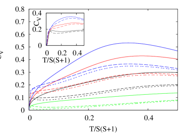
With increasing of $S$ there is a shift of the broad maximum typical for spin systems to lower values of the renormalized temperature $t=T/S(S+1)$ and an increase of its height, see Fig. 6. For fixed $S$ the frustration $J_{2}$ leads to a decrease of this maximum. Of particular interest is the low-temperature behavior of the specific heat. In Ref. haertel08, an additional frustration-induced low-temperature maximum in the specific heat was found for the $S=1/2$ model studied by RGM and ED. From Fig. 6 it is obvious that for higher values of $S$ this additional maximum disappears. Note that this observation is similar to the findings in Ref. ihle_new, for a field-induced low-temperature maximum in $C_{V}$, which appears for low values of $S$ only. To be more specific, we find that for $S>1$ no extra maximum appears in the RGM data for $C_{V}$ in the whole range of $0<J_{2}\leq 0.22$ accessible within the RGM approach. The frustration-induced low-temperature maximum for $S=1/2$ appears in the RGM for $J_{2}\geq 0.16$ (Ref. haertel08, ). For $S=1$ we find that a double-maximum structure in $C_{V}$ calculated by RGM appears for $J_{2}\geq 0.21$.

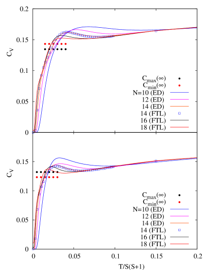
These RGM based results are supported by finite-size data (see inset of Fig. 6), i.e. we find also in the ED data for $N=8$ a clear tendency to suppress the extra low-temperature maximum if $S$ increases. In more detail we analyze finite-size data for $S=1$, where the larger systems are accessible by numerical methods. In Fig. 7 we illustrate the finite size-effects in $C_{V}$ for $S=1$ and $J_{2}=0.2$ and $0.22$. It is obvious that the extra low-temperature maximum is appreciably affected by finite-size effects. However, from Fig. 7 it is also evident that the height of the extra low-temperature maximum as well as the nearby minimum behave monotonously with $N$. Hence a finite-size extrapolation of the height $C_{max}(N)$ of the extra maximum and the related minimum $C_{min}(N)$ is reasonable. Analogously to Ref. haertel08, we find that $a(N)=a_{0}+a_{1}/N^{2}+a_{2}/N^{4}$ as a reasonable extrapolation scheme. The results of the extrapolation are shown in Fig. 7 by black [for the extrapolated value $C_{max}(\infty)$] and red [for the extrapolated value of $C_{min}(\infty)$] filled circles. These extrapolated data for $C_{max}$ and $C_{min}$ indicate, that there is most likely no extra low-temperature maximum for $J_{2}=0.2$, but such a maximum appears for $J_{2}=0.22$. Hence, the finite-size data support the RGM predictions that the double-peak structure appears for $S=1$ at $J_{2}\geq 0.21$.

V Summary

In this paper we have studied the influence of a frustrating NNN coupling $J_{2}$ on the thermodynamics of the 1D spin-$S$ $J_{1}$-$J_{2}$ Heisenberg model with ferromagnetic $J_{1}$ and antiferromagnetic $J_{2}$ with $J_{2}\leq|J_{1}|/4$. For that we have used the RGM for infinite chains and full ED as well as the FTL technique for finite chains. We find a universal dependence of the thermodynamic quantities on the renormalized temperature $t=T/S(S+1)$ at large temperatures. At low temperatures such a universal behavior is found for the critical properties of the susceptibility $\chi T^{2}/S^{4}=(2/3)(|J_{1}|-4J_{2})$ and the correlation length $\xi T/S^{2}=|J_{1}|-4J_{2}$, i.e., the critical exponents of $\chi$ and $\xi$ for $T\to 0$ are not changed by a frustrating $J_{2}<0.25|J_{1}|$. However, our data suggest that at the quantum critical point $J_{2}=|J_{1}|/4$ the critical behavior of $\chi$ and $\xi$ is changed.

For $S=1/2$ and $S=1$ an additional low-temperature maximum in the specific heat $C_{V}$ emerges when $J_{2}$ approaches the quantum critical point. Since we did not observe such an additional maximum in $C_{V}$ for $S>1$, it can be attributed to strong quantum fluctuations present at small values of $S$.

Acknowledgment: We thank the DFG for financial support (grants DR269/3-1 and RI615/16-1). Computing time at the Leibniz Computing Center in Garching is gratefully acknowledged.

References

- (1) H.P. Bader and R. Schilling, Phys. Rev. B 19, 3556 (1979).
- (2) A.V. Chubukov, Phys. Rev. B 44, 4693 (1991).
- (3) F. Heidrich-Meisner, A. Honecker, and T. Vekua, Phys. Rev. B 74 020403(R) (2006).
- (4) D.V. Dmitriev, V.Ya. Krivnov, and J. Richter, Phys. Rev. B 75, 014424 (2007).
- (5) D.V. Dmitriev and V.Ya. Krivnov, Phys. Rev. B 77, 024401 (2008).
- (6) T. Hikihara, T. Momoi , A. Furusaki, and H. Kawamura Phys. Rev. B 78, 144404 (2008).
- (7) M. Härtel, J. Richter, D. Ihle, and S.-L. Drechsler, Phys. Rev. B 78, 174412 (2008); J. Richter, M. Härtel, D. Ihle, and S.-L. Drechsler, J.Phys.:Conf.Ser. 145, 012064 (2009).
- (8) R. Zinke, S.-L. Drechsler, and J. Richter, Phys. Rev. B 79, 094425 (2009).
- (9) J. Sudan, A. Luscher, and A. Läuchli, Phys. Rev. B 80, 140402(R) (2009).
- (10) J. Sirker, Phys. Rev. B 81, 014419 (2010).
- (11) M. Härtel, J. Richter, and D. Ihle, arXiv:1102.3531 (accepted Phys.Rev.B).
- (12) S. Nishimoto, S.-L. Drechsler, R.O. Kuzian, J. van den Brink, J. Richter, Y. Skourski, W.E.A. Lorenz, R. Klingeler, and B. Büchner, arXiv:1004.3300 (2010) and Phys. Rev. Lett. (in press).
- (13) K. Kudo, S. Kurogi, Y. Koike, T. Nishizaki, and N. Kobayashi Phys. Rev. B 71, 104413 (2005).
- (14) S.-L. Drechsler, O. Volkova, A.N. Vasiliev, N. Tristan, J. Richter, M. Schmitt, H. Rosner, J. Málek, R. Klingeler, A.A. Zvyagin, and B. Büchner, Phys. Rev. Lett. 98, 077202 (2007).
- (15) J. Málek, S.-L. Drechsler, U. Nitzsche, H. Rosner, and H. Eschrig, Phys. Rev. B 78, 060508 (2008).
- (16) C.P. Landee and R.D. Willett, Phys. Rev. Lett. 43, 463 (1979); C. Dupas, J.P. Renard, J. Seiden, and A. Cheikh-Rouhou, Phys. Rev. B 25, 3261 (1982).
- (17) J. K. Kjems and M. Steiner, Phys. Rev. Lett. 41, 1137 (1978); T. Delica, W.J. de Jonge, K. Kopinga, H. Leschke, and H.J. Mikeska, Phys. Rev. B 44, 11773 (1991).
- (18) W. Zhang, C. P. Landee, M. M. Turnbull, and R. D. Willett, J. Appl. Phys. 73, 5379 (1993)
- (19) P. Gambardella, A. Dallmeyer, K. Maiti, M.C. Malagoli, W. Eberhardt, K. Kern, and C. Carbone, Nature 416, 301 (2002); A. Vindigni, A. Rettori, M.G. Pini, C. Carbone, and P. Gambardella, Appl. Phys. A 82, 385 (2006).
- (20) F.D.M. Haldane, Phys. Lett. A 93, 464 (1983); Phys. Rev. Lett. A 50, 1153 (1983).
- (21) I. Juhász Junger, D. Ihle, L. Bogacz, and W. Janke, Phys. Rev. B 77, 174411 (2008).
- (22) I. Junger, D. Ihle, J. Richter, and A. Klümper, Phys. Rev. B 70, 104419 (2004).
- (23) T.N. Antsygina, M.I. Poltavskaya, I.I. Poltavsky, and K.A. Chishko, Phys. Rev. B 77, 024407 (2008).
- (24) M. Härtel, J. Richter, D. Ihle, and S.-L. Drechsler, Phys. Rev. B 81, 174421 (2010).
- (25) D.V. Dmitriev and V.Y. Krivnov, Phys. Rev. B 82, 054407 (2010); arXiv:1007.4536 (unpublished)
- (26) J. Kondo and K. Yamaji, Prog. Theor. Phys. 47, 807 (1972); H. Shimahara and S. Takada, J. Phys. Soc. Jpn. 60, 2394 (1991); S. Winterfeldt and D. Ihle, Pys. Rev. B 56, 5535 (1997).
- (27) F. Suzuki, N. Shibata, and C. Ishi, J. Phys. Soc. Jpn. 63, 1539 (1994).
- (28) W. Yu and S. Feng, Eur. Phys. J. B 13, 265 (2000); L. Siurakshina, D. Ihle, and R. Hayn, Phys. Rev. B 64, 104406 (2001); B.H. Bernhard, B. Canals, and C. Lacroix, Phys. Rev. B 66, 024422 (2002); D. Schmalfuß, J. Richter, and D. Ihle, Phys. Rev. B 70, 184412 (2004); D. Schmalfuß, J. Richter, and D. Ihle, Phys. Rev. B 72, 224405 (2005); D. Schmalfuß, R. Darradi, J. Richter, J. Schulenburg, and D. Ihle, Phys. Rev. Lett. 97, 157201 (2006).
- (29) I. Juhász Junger, D. Ihle, and J. Richter, Phys. Rev. B 72, 064454 (2005).
- (30) I. Juhász Junger, D. Ihle, and J. Richter, Phys. Rev. B 80, 064425 (2009).
-
(31)
J. Schulenburg, program package spinpack,
http:://www-e.uni-magdeburg.de/jschulen/spin/ - (32) W. Gasser, E. Heiner and K. Elk, Greensche Funktionen in Festkörper- und Vielteilchenphysik (WILEY-VCH Verlag, Berlin 2001).
- (33) J. Jaklic and P. Prelovsek, Phys. Rev. B 49, 5065 (1994); Adv. Phys. 49, 1 (2000).
- (34) J. Schnack and O. Wendland, Eur. Phys. J. B 78, 535 (2010).
- (35) H.-J. Mikeska and A.K. Kolezhuk, in Quantum Magnetism, eds. U. Schollwöck, J. Richter, D.J.J. Farnell, and R.F. Bishop, Eds., Lecture Notes in Physics 645 (Springer, Berlin, 2004), p. 1.
- (36) T. Hamada, J. Kane, S. Nakagawa, and Y. Natsume, J. Phys. Soc. Jpn. 57, 1891 (1988); 58, 3869 (1989).
- (37) G.S. Rushbrooke, G.A. Baker, and P.J. Wood, in Phase Transitions and Critical Phenomena, Vol. 3, p. 245; eds. C. Domb and M.S. Green, Academic Press, london, 1974.
- (38) J. Oitmaa, C.J. Hamer, and W.H. Zheng, Series Expansion Methods. Cambridge University Press, 2006.
- (39) M. Takahashi, Prog. Theor. Phys. Supp. 87, 233 (1986); M. Takahashi, Phys. Rev. Lett. 58 168 (1987).
- (40) M. Yamada, J. Phys. Soc. Jpn. 59, 848 (1990).
- (41) M. Yamada and M. Takahashi, J. Phys. Soc. Jpn. 55, 2024 (1986).
- (42) P. Kopietz and G. Castilla, Phys. Rev. B 43 11100 (1991).
- (43) N.B. Ivanov, Condens. Matter Phys. (L’viv) 12, 435 (2009) (see also arXiv:0909.2182).
- (44) J. Sirker, V.Y. Krivnov, D.V. Dmitriev, A. Herzog, S. Nishimoto, S.-L. Drechsler, O. Janson, and J. Richter, in preparation.