Critical gravity on AdS2 spacetimes


Yun Soo Myung1,a, Yong-Wan Kim 1,b, and Young-Jai Park2,c


1Institute of Basic Science and School of Computer Aided Science,

Inje University, Gimhae 621-749, Korea

2Department of Physics and Department of Service Systems Management and Engineering,

Sogang University, Seoul 121-742, Korea

Abstract

We study the critical gravity in two dimensional AdS (AdS2) spacetimes, which was obtained from the cosmological topologically massive gravity (TMGΞ›) in three dimensions by using the Kaluza-Klein dimensional reduction. We perform the perturbation analysis around AdS2, which may correspond to the near-horizon geometry of the extremal BTZ black hole obtained from the TMGΞ› with identification upon uplifting three dimensions. A massive propagating scalar mode $\delta F$ satisfies the second-order differential equation away from the critical point of $K=l$, whose solution is given by the Bessel functions. On the other hand, $\delta F$ satisfies the fourth-order equation at the critical point. We exactly solve the fourth-order equation, and compare it with the log-gravity in two dimensions. Consequently, the critical gravity in two dimensions could not be described by a massless scalar $\delta F_{\rm ml}$ and its logarithmic partner $\delta F^{\rm 4th}_{\rm log}$.

PACS numbers: 04.70.Bw, 04.60.Rt, 04.60.Kz, 04.70.-s
Keywords: Critical gravity; Topologically massive gravity; 2D dilaton gravity; BTZ black holes.


aysmyung@inje.ac.kr
bywkim65@gmail.com
cyjpark@sogang.ac.kr

1 Introduction

The gravitational Chern-Simons (gCS) terms in three dimensional (3D) Einstein gravity produce a physically propagating massive graviton [1]. This topologically massive gravity with a negative cosmological constant $\Lambda=-1/l^{2}$ (TMGΞ› [2]) gives us the AdS3 solution [3]. For the positive Newton’s constant $G_{3}$, a massive graviton mode carries ghost (negative energy) on the AdS3. In this sense, the AdS3 is not a stable vacuum. The opposite case of $G_{3}<0$ may cure the problem, but it may induce a negative Deser-Tekin mass for the BTZ black hole [4]. It seems that there is one way of avoiding negative energy by choosing the chiral (critical) point of $K=l$ with the gCS coupling constant $K$. At this point, a massive graviton becomes a massless left-moving graviton, which carries no energy. It may be considered as gauge-artefact. However, the critical point has raised many questions on physical degrees of freedom (DOF) [5, 6, 7, 8, 9, 10, 11, 12].

The gCS terms are not invariant under coordinate transformations though they are conformally invariant [13, 14]. It is known that the 3D Einstein gravity is locally trivial, and thus, does not have any physically propagating modes. However, all solutions to the Einstein gravity are also solutions to the TMGΞ›. Therefore, it would be better to seek another method to find a propagating massive mode in the TMGΞ› since it is likely a candidate for a nontrivial 3D gravity, in addition to the new massive gravity [15]. To this end, one may introduce a conformal transformation and then, the Kaluza-Klein reduction can be used to obtain an effective two-dimensional action (2DTMGΞ›), which becomes a gauge and coordinate invariant action. Saboo and Sen [16, 17] have used the 2DTMGΞ› to derive the entropy of extremal BTZ black hole [18] by using the entropy function formalism (AdS2 attractor equation). When using the Achucarro-Ortiz type of dimensional reduction, it turned out that there is no propagating massive mode on AdS2 background [19].

In this work, we will focus on the chiral point of $K=l$, where a massive graviton $\psi^{M}_{mn}$ turned out to be a left-moving graviton $\psi^{L}_{mn}$ [3, 20]. Grumiller and Johanson have introduced a new field $\psi^{\rm new}_{mn}=\partial_{l/K}\psi^{M}_{mn}|_{K=l}$ as a logarithmic parter of $\psi^{L}_{mn}$ [6] based on the logarithmic conformal field theory (LCFT) with $c_{L}=0$ [21, 22, 23, 24]. However, it was reported that $\psi^{\rm new}_{mn}$ might not be a physical field at the chiral point, since it belongs to the nonunitary theory. This is so because $(\psi^{L}_{mn},\psi^{\rm new}_{mn})$ become a pair of dipole ghost fields [25]. At this stage, we would like to mention that the linearized higher dimensional critical gravities were recently investigated in the AdS spacetimes [26], but the nonunitary issue of the log-gravity is not still resolved, indicating that the log-gravity suffers from the ghost problem.

A few years ago, we have carried out perturbation analysis of the 2DTMGΞ› around AdS2 background [27]. We have shown that the dual scalar $\delta F$ of the Maxwell field is a gauge-invariant massive mode propagating in the AdS2 background. Recently, we have studied the critical gravity arisen from the new massive gravity by investigating quasinormal modes to check the stability of the BTZ black hole [28].

Hence it is interesting to study the critical gravity arisen from the 2DTMGΞ›, which shows a fourth-order differential equation on AdS2 background.

The organization of our work ia as follows. In Section 2, we study the 2DTMGΞ›, which was obtained from the TMGΞ› by using the Kaluza-Klein dimensional reduction. In Section 3, we briefly review the perturbation analysis around AdS2, which may correspond to the near-horizon geometry of the extremal BTZ black hole obtained from the TMGΞ› with identification upon uplifting three dimensions. We find an explicit solution of a physically propagating scalar mode $\delta F$ satisfying the second-order differential equation away from the critical point of $K=l$. At the critical point, in Section 4, the 2DTMGΞ› turns out to be the 2D dilaton gravity including the Maxwell field obtained from 3D Einstein gravity, which shows that there are no propagating modes. We exactly solve the fourth order equation at the critical point, and compare it with the log-gravity ansatz in two dimensions. Discussion is given in Section 5.

2 2DTMGΞ›

We start with the action for the TMGΞ› given by [1]

$$I_{\rm TMG_{\Lambda}}=\frac{1}{16\pi G_{3}}\int d^{3}x\sqrt{-g}\Bigg{[}R_{3}-2\Lambda-\frac{K}{2}\varepsilon^{lmn}\Gamma^{p}_{~{}lq}\Big{(}\partial_{m}\Gamma^{q}_{~{}np}+\frac{2}{3}\Gamma^{q}_{~{}mr}\Gamma^{r}_{~{}np}\Big{)}\Bigg{]},$$ (1)

where $\varepsilon$ is the tensor defined by $\epsilon/\sqrt{-g}$ with $\epsilon^{012}=1$. We choose the positive Newton’s constant $G_{3}>0$ and the negative cosmological constant $\Lambda=-1/l^{2}$. The Latin indices of $l,m,n,\cdots$ denote three dimensional tensors. The $K$-term is called the gCS terms. Here we choose β€œβˆ’-” sign in the front of $K$ [17]. Varying this action leads to the Einstein equation

$$G_{mn}-KC_{mn}=0,$$ (2)

where the Einstein tensor is given by

$$G_{mn}=R_{3mn}-\frac{R_{3}}{2}g_{mn}-\frac{1}{l^{2}}g_{mn},$$ (3)

and the Cotton tensor is defined by

$$C_{mn}=\varepsilon_{m}~{}^{pq}\nabla_{p}\Big{(}R_{3qn}-\frac{1}{4}g_{qn}R_{3}\Big{)}.$$ (4)

We note that the Cotton tensor $C_{mn}$ vanishes for any solution to the 3D Einstein gravity, so all solutions of the Einstein gravity are also solutions of the TMGΞ›. Hence, the BTZ black hole with $K=0$ [18] appears as a solution to the full equation (2)

$$ds^{2}_{\rm BTZ}=-N^{2}(r)dt^{2}+\frac{dr^{2}}{N^{2}(r)}+r^{2}\Big{[}d\theta+N^{\theta}(r)dt\Big{]}^{2},$$ (5)

where the squared lapse $N^{2}(r)$ and the angular shift $N^{\theta}(r)$ take the forms

$$N^{2}(r)=-8G_{3}m+\frac{r^{2}}{l^{2}}+\frac{16G_{3}^{2}j^{2}}{r^{2}},~{}~{}N^{\theta}(r)=-\frac{4G_{3}j}{r^{2}}.$$ (6)

Here $m$ and $j$ are the mass and angular momentum of the BTZ black hole, respectively.

We first make a conformal transformation and then perform Kaluza-Klein dimensional reduction by choosing the metric [13, 14]

$$ds^{2}_{\rm KK}=\phi^{2}\Big{[}g_{\mu\nu}(x)dx^{\mu}dx^{\nu}+\Big{(}d\theta+A_{\mu}(x)dx^{\mu}\Big{)}^{2}\Big{]}$$ (7)

because the gCS terms are invariant under the conformal transformation. Here $\theta$ is a coordinate that parameterizes an $S^{1}$ with a period $2\pi l$. Hence, its isometry is factorized as ${\cal G}\times U(1)$. After the β€œΞΈπœƒ\theta”-integration, the action (1) reduces to an effective two-dimensional action called the 2DTMGΞ› as

$\displaystyle I_{\rm 2DTMG_{\Lambda}}$ $\displaystyle=$ $\displaystyle\frac{l}{8G_{3}}\int d^{2}x\sqrt{-g}\left(\phi R+\frac{2}{\phi}g^{\mu\nu}\nabla_{\mu}\phi\nabla_{\nu}\phi+\frac{2}{l^{2}}\phi^{3}-\frac{1}{4}\phi F_{\mu\nu}F^{\mu\nu}\right)$ (8)
$\displaystyle-$ $\displaystyle\frac{Kl}{32G_{3}}\int d^{2}x\left(R\epsilon^{\mu\nu}F_{\mu\nu}+\epsilon^{\mu\nu}F_{\mu\rho}F^{\rho\sigma}F_{\sigma\nu}\right),$

which is our main action to study the critical gravity in two dimensions. Here $R$ is the 2D Ricci scalar with $R_{\mu\nu}=Rg_{\mu\nu}/2$, and $\phi$ is a dilaton. Also, the Maxwell field is defined by $F_{\mu\nu}=2\partial_{[\mu}A_{\nu]}$, and $\epsilon^{\mu\nu}$ is a tensor density. The Greek indices of $\mu,\nu,\rho,\cdots$ represent two dimensional tensors. Hereafter we choose $G_{3}=l/8$ for simplicity. It is again noted that this action was actively used to derive the entropy of extremal BTZ black hole by applying the entropy function approach [16, 17, 27]. Introducing a dual scalar $F$ of the Maxwell field defined by [13, 14]

$$F\equiv-\frac{1}{2\sqrt{-g}}\epsilon^{\mu\nu}F_{\mu\nu},$$ (9)

equations of motion for $\phi$ and $A_{\mu}$ are given, respectively, by

$\displaystyle R+\frac{2}{\phi^{2}}(\nabla\phi)^{2}-\frac{4}{\phi}\nabla^{2}\phi+\frac{6}{l^{2}}\phi^{2}+\frac{1}{4}F^{2}=0,$ (10)
$\displaystyle\epsilon^{\mu\nu}\partial_{\nu}\left[\phi F+\frac{K}{2}(R+3F^{2})\right]=0.$ (11)

The equation of motion for the metric $g_{\mu\nu}$ takes the form

$\displaystyle g_{\mu\nu}\left(\nabla^{2}\phi-\frac{1}{l^{2}}\phi^{3}+\frac{1}{4}\phi F^{2}-\frac{1}{\phi}(\nabla\phi)^{2}\right)+\frac{2}{\phi}\nabla_{\mu}\phi\nabla_{\nu}\phi-\nabla_{\mu}\nabla_{\nu}\phi$
$\displaystyle+\frac{K}{2}\left[g_{\mu\nu}\left(\nabla^{2}F+F^{3}+\frac{1}{2}RF\right)-\nabla_{\mu}\nabla_{\nu}F\right]=0.$ (12)

The trace part of Eq. (2)

$$\nabla^{2}\phi-\frac{2}{l^{2}}\phi^{3}+\frac{1}{2}\phi F^{2}+K\left(\frac{1}{2}RF+F^{3}+\frac{1}{2}\nabla^{2}F\right)=0$$ (13)

is relevant to our perturbation study. On the other hand, the traceless part is given by

$$g_{\mu\nu}\left(\frac{1}{2}\nabla^{2}\phi-\frac{1}{\phi}(\nabla\phi)^{2}\right)+\frac{2}{\phi}\nabla_{\mu}\phi\nabla_{\nu}\phi-\nabla_{\mu}\nabla_{\nu}\phi+\frac{K}{4}g_{\mu\nu}\nabla^{2}F-\frac{K}{2}\nabla_{\mu}\nabla_{\nu}F=0$$ (14)

which may provide a redundant constraint [19]. Now, we are in a position to find AdS2 spacetimes as a vacuum solution to (10), (11), and (13). In case of a constant dilaton, from (10) and (13), we have the condition of a vacuum state

$$(3KF+2\phi)\left(\frac{\phi^{2}}{l^{2}}-\frac{1}{4}F^{2}\right)=0,$$ (15)

which provides two distinct relations between $\phi$ and $F$

$\displaystyle\phi_{\pm}=\pm\frac{l}{2}F.$ (16)

Assuming the line element preserving ${\cal G}=SL(2,R)$ isometry

$$ds^{2}_{\rm AdS_{2}}=\bar{g}_{\mu\nu}dx^{\mu}dx^{\nu}=v\left(-r^{2}dt^{2}+\frac{dr^{2}}{r^{2}}\right),$$ (17)

we have the AdS2 spacetimes, which satisfy

$$\bar{R}=-\frac{2}{v},~{}~{}~{}\bar{\phi}=u,~{}~{}~{}\bar{F}=\frac{e}{v~{}}(\bar{F}_{10}=e).$$ (18)

Here $\bar{F}_{10}=\partial_{1}\bar{A}_{0}-\partial_{0}\bar{A}_{1}$ with $\bar{A}_{0}=er$ and $\bar{A}_{1}=0$. This background may correspond to the near-horizon geometry of the extremal BTZ black hole (NHEB), factorized as AdS${}_{2}\times S^{1}$ as

$$ds^{2}_{\rm\pm NHEB}=\frac{l^{2}}{4}\Bigg{[}-r^{2}dt^{2}+\frac{dr^{2}}{r^{2}}+(dz\mp rdt)^{2}\Bigg{]},$$ (19)

where $v=l^{2}/4$ and $z=l\theta/|e|$ with the identification of $z\sim 2\pi ln\frac{l}{|e|}$. Here $n$ is an integer. As was pointed out in Ref. [29], the NHEB is a self-dual orbifold of AdS3. This geometry has a null circle on its boundary and thus, the dual conformal field theory is a Discrete Light Cone Quantized (DLCQ) of CFT2. The kinematics of the DLCQ show that in a consistent quantum field theory of gravity in these backgrounds, there is no dynamics in AdS2, which is consistent with the Kaluza-Klein reduction of the 3D Einstein gravity. However, the gCS terms in the TMGΞ› are odd under parity, and as a result, the theory shows a single massive propagating degree of freedom of a given helicity, whereas the other helicity mode remains massless. The single massive field is realized as a massive scalar $\varphi=z^{3/2}h_{zz}$ when using the Poincare coordinates $x^{\pm}$ and $z$ covering the AdS3 spacetimes [5, 10]. We have shown that a propagating massive mode is a dual scalar $\delta F$ of the Maxwell field on a self dual orbifold of AdS3 (AdS2 background) [27].

3 Perturbation around AdS2

We briefly review the perturbation around the AdS2 and find the explicit form of a massive propagating mode. Let us first consider the perturbation modes of the dilaton, graviton, and dual scalar around the AdS2 background as

$\displaystyle\phi$ $\displaystyle=$ $\displaystyle\bar{\phi}+\varphi,$ (20)
$\displaystyle g_{\mu\nu}$ $\displaystyle=$ $\displaystyle\bar{g}_{\mu\nu}+h_{\mu\nu},~{}~{}h_{\mu\nu}=-h\bar{g}_{\mu\nu}$ (21)
$\displaystyle F$ $\displaystyle=$ $\displaystyle\bar{F}(1+\delta F),~{}~{}\delta F=\left(h-\frac{f}{e}\right)$ (22)

where the bar variables denote the AdS2 background (17) and (18). The Maxwell field has a scalar perturbation $f$ around the background: $F_{10}=\bar{F}_{10}+\delta F_{10}$, where $\delta F_{10}=-f$. We note that two scalars of $\delta F$ and $\varphi$ are gauge-invariant quantities in AdS2 spacetimes although $f$ is not [27]. Then, considering $\delta R(h)=\bar{\nabla}^{2}h-\frac{2}{v}h$, the perturbed equations of motion to (10), (11) and (13) are given, respectively, by

$\displaystyle\bar{\nabla}^{2}h-\frac{2}{v}h-\frac{4}{u}\bar{\nabla}^{2}\varphi+\frac{12}{l^{2}}u\varphi+\frac{e^{2}}{v^{2}}\delta F=0,$ (23)
$\displaystyle\epsilon^{\mu\nu}\partial_{\nu}\Bigg{[}\frac{e}{v}\Big{(}\varphi+u\delta F\Big{)}+\frac{K}{2}\Big{(}\bar{\nabla}^{2}h-\frac{2}{v}h+\frac{6e^{2}}{v^{2}}\delta F\Big{)}\Bigg{]}=0,$ (24)
$\displaystyle\bar{\nabla}^{2}\varphi-\frac{6}{l^{2}}u^{2}\varphi+\frac{e^{2}}{2v^{2}}\varphi+\frac{ue^{2}}{v^{2}}\delta F$
$\displaystyle+K\Bigg{(}\frac{e}{2v}\bar{\nabla}^{2}h-\frac{e}{v^{2}}h+\frac{e(3e^{2}-v)}{v^{3}}\delta F+\frac{e}{2v}\bar{\nabla}^{2}\delta F\Bigg{)}=0.$ (25)

Solving (24) for $\delta F$ and inserting it into Eq. (3) leads to

$$\left(\bar{\nabla}^{2}-\frac{2}{v}\right)\left(\varphi+\frac{Ke}{2v}\delta F\right)=0$$ (26)

Also, solving (24) for $(\bar{\nabla}^{2}-\frac{2}{v})h$ and then, inserting it into Eq. (23) arrives at

$$\left(\bar{\nabla}^{2}-\frac{2}{v}\right)\varphi-\left(\frac{ue}{2vK}+\frac{5}{4v}\right)\Big{(}\varphi+u\delta F\Big{)}=0.$$ (27)

Making use of (26) and (27), $\delta F$ and $\varphi$ satisfy the coupled equation

$$\left(\bar{\nabla}^{2}-\frac{2}{v}\right)\delta F-\frac{2v}{Ke}\left(\frac{ue}{2vK}+\frac{5}{4v}\right)\Big{(}\varphi+u\delta F\Big{)}=0,$$ (28)

Acting $\left(\bar{\nabla}^{2}-\frac{2}{v}\right)$ on (28), and then eliminating $\varphi$ again by using (26), one finds the fourth-order equation for $\delta F$ as follows

$$\left(\bar{\nabla}^{2}-\frac{2}{v}\right)\left[\bar{\nabla}^{2}-\left(\frac{2}{v}+m^{2}_{\pm}\right)\right]\delta F=0,$$ (29)

for the two AdS2 solutions of $u=\pm\ell e/2v$ in (16). Here, the mass squared $m^{2}_{\pm}$ is given by

$$m^{2}_{\pm}=\frac{1}{4v}\left(\pm\frac{l}{K}-1\right)\left(5\pm\frac{l}{K}\right).$$ (30)

Here we stress that our mass squared is defined differently from the Ref. [27].
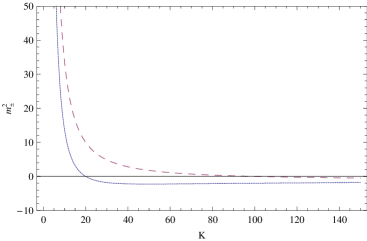
Refer to caption
Figure 1: Mass $m^{2}_{\pm}$ for the AdS2 solution for $l=100$ and $v=1$: The dotted curve is for the negative mass squared $m^{2}_{-}$, while the dashed curve is for the positive mass squared $m^{2}_{+}=m^{2}$. Since the AdS2 solution with a positive charge $q$ is valid for $K\leq l$ [17], the permitted region is $0\leq K\leq 100$.

For $0\leq K\leq l$, one requires $m^{2}\geq 0$, which selects $m^{2}_{+}\equiv m^{2}$ (see Fig. 1). Hereafter we consider this case only. For m2β‰ 0superscriptπ‘š20m^{2}\neq 0, the fourth order equation (29) implies two second order equations: one is for a massless field

$$\left[\bar{\nabla}^{2}-\frac{2}{v}\right]\delta F=0,$$ (31)

while the other is for a massive scalar

$$\left[\bar{\nabla}^{2}-\left(\frac{2}{v}+m^{2}\right)\right]\delta F=0,$$ (32)

In order to solve the massive equation (32), we transform the AdS2 metric as

$\displaystyle ds^{2}_{\rm AdS_{2}}$ $\displaystyle=$ $\displaystyle v\left(-r^{2}dt^{2}+\frac{dr^{2}}{r^{2}}\right)$ (33)
$\displaystyle\to$ $\displaystyle-\left(\frac{x^{2}}{v}\right)dt^{2}+\left(\frac{v}{x^{2}}\right)dx^{2}$ (34)
$\displaystyle\to$ $\displaystyle\frac{ds^{2}}{v}=\left(\frac{1}{x^{2}_{*}}\right)\Big{[}-dt^{2}+dx^{2}_{*}\Big{]},$ (35)

in the second line, we used $x=vr$, and in the last line, $x_{*}=v/x=1/r$. We note that in the last line, $(t,x_{*})$ corresponds to the PoincarΓ© coordinates $(T,y)$ used in Ref. [30] to construct the Hadamard Green function for the PoincarΓ©.

Finally, we wish to find a positive frequency mode for $\delta F$ as

$$\delta F(t,x_{*})=e^{-i\omega t}\delta f(x_{*}).$$ (36)

Then, the second-order equation (32) becomes

$$\frac{d^{2}}{dx^{2}_{*}}\delta f+\left[\omega^{2}-\frac{(m^{2}v+2)}{x^{2}_{*}}\right]\delta f=0,$$ (37)

whose solution is given by the Bessel functions

$$\delta f(x_{*})=c_{1}\sqrt{x_{*}}J_{\nu}(\omega x_{*})+c_{2}\sqrt{x_{*}}Y_{\nu}(\omega x_{*})$$ (38)

where $\nu={\sqrt{m^{2}v+\frac{9}{4}}}$ satisfying $\nu^{2}-1/4=m^{2}v+2$. Also, we observe that the event horizon is located at $r\to 0~{}(x_{*}\to\infty)$, while the infinity is located at $r\to\infty~{}(x_{*}\to 0)$. In order to have the normalizable solution, we choose $c_{2}=0$ because $Y_{\nu}(\omega x_{*})$ blows up at $x_{*}=0$.

4 Critical gravity in two dimensions

At the critical point of $m^{2}=0~{}(K=l)$, (29) becomes the fourth-order differential equation

$$\left(\bar{\nabla}^{2}-\frac{2}{v}\right)^{2}\delta F^{\rm 4th}=0.$$ (39)

In order to solve this equation, first of all, we observe that the Bessel function of order $\nu=3/2$ satisfies the second-order equation for a massless scalar on AdS2 spacetimes as follows:

$\displaystyle\left(\bar{\nabla}^{2}-\frac{2}{v}\right)\delta F_{\rm ml}=0,$ (40)

whose normalizable solution is given by

$$\delta F_{\rm ml}(t,x_{*})=e^{-i\omega t}\delta f_{\rm ml}(x_{*})$$ (41)

where

$$\delta f_{\rm ml}(x_{*})\simeq\sqrt{x_{*}}J_{3/2}(\omega x_{*})=\sqrt{\frac{2}{\pi\omega}}\Bigg{[}-\cos(\omega x_{*})+\frac{\sin(\omega x_{*})}{\omega x_{*}}\Bigg{]}.$$ (42)

At this stage, we remind the reader that two equations (39) and (40) with $K=l$ are the same equations

$$\left(\bar{\nabla}^{2}-\frac{2}{v}\right)^{2}h=0,~{}~{}\left(\bar{\nabla}^{2}-\frac{2}{v}\right)\varphi=0.$$ (43)

for the graviton and dilaton as found from the 3D Einstein gravity with $K=0$ [27]. Here we observe the important correspondence as

$$\delta F_{\rm ml}\leftrightarrow\varphi,~{}~{}~{}\delta F^{\rm 4th}\leftrightarrow h.$$ (44)

In the 3D linearized Einstein gravity, one confirms the connection between dilaton and dual scalar

$$\frac{\varphi}{u}=-\delta F.$$ (45)

This means that there are no propagating massive modes at the critical point, showing apparently that all modes of $h,\varphi,$ and $\delta F$ from the 3D Einstein gravity are gauge-artefacts. However, it was proposed that any critical gravity has a new field on AdS spacetimes. In order to explore this idea on the AdS2 spacetimes, we consider a positive frequency fourth-order field

$$\delta F^{\rm 4th}(t,x_{*})=e^{-i\omega t}\delta f^{\rm 4th}(x_{*}).$$ (46)

Then, the fourth order equation (39) takes the form

$$\left[\frac{d^{2}}{dx^{2}_{*}}+\left(\omega^{2}-\frac{2}{x^{2}_{*}}\right)\right]^{2}\delta f^{\rm 4th}=0.$$ (47)

Replacing $\omega x_{*}=\omega/r$ by $r_{*}$ and considering

$$\delta f^{\rm 4th}(r_{*})=g(r_{*})\delta f_{\rm ml}(r_{*}),$$ (48)

(47) reduces to the second-order equation for $g(r_{*})$ as

$$\Big{[}g^{\prime\prime}(r_{*})-1\Big{]}=-\frac{2\delta f^{\prime}_{\rm ml}(r_{*})}{\delta f_{\rm ml}(r_{*})}g^{\prime}(r_{*}),$$ (49)

where the prime β€² denotes the differentiation with respect to its argument. Plugging (42) into (49) leads to the exact solution for $g(r_{*})$

$$g(r_{*})=C_{2}+\frac{2C_{1}\cos(r_{*})+r_{*}(r_{*}+2C_{1})\sin(r_{*})}{2[r_{*}\cos(r_{*})-\sin(r_{*})]}$$ (50)

with two undetermined parameters $C_{1}$ and $C_{2}$. Hereafter we set $C_{1}=-1$ and $C_{2}=1$ for simplicity. Now, making use of the two identities

$\displaystyle\sin(r_{*})$ $\displaystyle=$ $\displaystyle\sqrt{\frac{\pi}{2}}\left(\frac{3}{2\sqrt{x}}J_{3/2}(r_{*})+\sqrt{r_{*}}J^{\prime}_{3/2}(r_{*})\right),$
$\displaystyle\cos(r_{*})$ $\displaystyle=$ $\displaystyle\sqrt{\frac{\pi}{2}}\left(\frac{(3-2r^{2}_{*})}{2r^{3/2}_{*}}J_{3/2}(r_{*})+\frac{1}{\sqrt{r_{*}}}J^{\prime}_{3/2}(r_{*})\right),$ (51)

we have finally obtained a solution to the fourth-order equation (47) as

$$\delta f^{\rm 4th}(r_{*})=-\left(\frac{3+r^{2}_{*}-\frac{1}{2}r^{3}_{*}}{2r^{5/2}_{*}}\right)J_{3/2}(r_{*})-\left(\frac{1+r^{2}_{*}+\frac{1}{2}r^{3}_{*}}{r^{3/2}_{*}}\right)J^{\prime}_{3/2}(r_{*}),$$ (52)

where $J^{\prime}_{3/2}(r_{*})$ can be expressed in terms of the lower order Bessel functions as

$$J^{\prime}_{3/2}(r_{*})=\Big{(}1-\frac{3}{r_{*}^{3}}\Big{)}J_{1/2}+\frac{2}{2r_{*}^{3/2}}J_{-1/2}.$$ (53)

This shows that $J^{\prime}_{3/2}(r_{*})$ does not contain any singularity at infinity $r=\infty~{}(r_{*}=0)$. Fig. (2a) shows its behavior on $r_{*}$ clearly. To see it more explicitly, $g(r_{*})$ takes a series form near $r_{*}\sim 0~{}(r\rightarrow\infty)$

$$g(r_{*})\simeq-\frac{3}{r^{3}_{*}}-\frac{9}{5r_{*}}-\frac{1}{2}+\frac{36}{175}r_{*}+\frac{1}{10}r^{2}_{*}+\frac{47}{7875}r_{*}^{3}+\frac{1}{350}r^{4}_{*}\cdots.$$ (54)

Therefore, $\delta f^{\rm 4th}(r_{*})$ shows a negative infinity as

$$-\frac{1}{r_{*}}~{}~{}{\rm as}~{}~{}r_{*}\to 0$$ (55)

by observing the first term of

$$\delta f^{\rm 4th}(r_{*})=g(r_{*})\delta f_{\rm ml}(r_{*})\simeq\sqrt{\frac{2}{\pi}}\Bigg{(}-\frac{1}{r_{*}}-\frac{r_{*}}{2}-\frac{r_{*}^{2}}{6}+\frac{r^{3}_{*}}{8}+\frac{r^{4}_{*}}{20}-\frac{r^{5}_{*}}{144}-\frac{r^{6}_{*}}{336}\cdots\Bigg{)}.$$ (56)

For $C_{1}=-1$ and $C_{2}=1$, we have a positive infinity of $\delta f^{\rm 4th}(r_{*})\to\frac{1}{r_{*}}$ as $r_{*}\to 0$.

Refer to caption
Figure 2: Graphs of two functions $\delta f^{\rm 4th}(r_{*})$ and the logarithmic partner $\delta f^{\rm 4th}_{\rm log}(r_{*})$ of a normalizable function $\delta f_{\rm ml}(r_{*})=\sqrt{r_{*}}J_{3/2}(r_{*})$. Although the former is a truly solution to the fourth-order equation (47), it shows singular behavior at infinity of $r\to\infty~{}(r_{*}\to 0)$, which may not be acceptable as a true solution. On the other hand, even though the logarithmic partner $\delta f^{\rm 4th}_{\rm log}(r_{*})$ approaches zero at $r_{*}=0$, but it is unlikely a solution to the fourth-order equation (47).

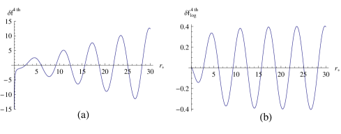
On the other hand, inspired by the log-gravity [6, 25], we suggest that a solution to the fourth-order equation (47) may take the form as a logarithmic partner of $\delta F_{\rm ml}$ [31]

$$\delta F^{\rm 4th}_{\rm log}(r_{*})=e^{-i\omega t}\delta f^{\rm 4th}_{\rm log}(r_{*}),$$ (57)

where

$\displaystyle\delta f^{\rm 4th}_{\rm log}(r_{*})$ $\displaystyle=$ $\displaystyle\left.\frac{\partial}{\partial m^{2}}\{\sqrt{r_{*}}J_{\nu}(r_{*})\}\right|_{m^{2}=0}$ (58)
$\displaystyle=$ $\displaystyle\frac{v\sqrt{r_{*}}}{3}\Bigg{[}J_{3/2}(r_{*})\ln(r_{*}/2)-\Big{(}\frac{r_{*}}{2}\Big{)}^{3/2}\sum^{\infty}_{k=0}(-1)^{k}\frac{\psi(5/2+k)}{\Gamma(5/2+k)}\frac{(\frac{1}{4}r^{2}_{*})^{k}}{k!}\Bigg{]}.$

Here $\Gamma(z)$ is the Gamma function and $\psi(z)$ is a diagamma function defined by $\psi(z)=\frac{d\ln\Gamma(z)}{dz}$. Fig. (2b) describes $\delta f^{\rm 4th}_{\rm log}(r_{*})$. In the case of $r_{*}\to 0$, one has a series form for $\delta f^{\rm 4th}_{\rm log}(r_{*})$ as

$\displaystyle\delta f^{\rm 4th}_{\rm log}(r_{*})$ $\displaystyle\simeq$ $\displaystyle\frac{v}{27}\sqrt{\frac{2}{\pi}}\Bigg{(}[-8+3\gamma+3\ln(2r_{*})]r_{*}^{2}-\frac{[-46+15\gamma+15\ln(2r_{*})]r_{*}^{4}}{50}$ (59)
$\displaystyle~{}~{}~{}~{}~{}~{}~{}~{}~{}~{}+\frac{[-352+105\gamma+105\ln(2r_{*})]r_{*}^{6}}{9800}+\cdots\Bigg{)}$

with $\gamma$ the Euler constant. From this form, we find that $\delta f^{\rm 4th}_{\rm log}(r_{*})$ approaches zero as $r_{*}\to 0$ even though the logarithmic terms are present. Applying the l’Hospital’s rule to $r^{n}_{*}\ln(r_{*}/2)$ with $n\geq 1$ [equivalently, $J_{3/2}(r_{*})\ln(r_{*}/2)]$ as $r_{*}\to 0$, one finds immediately that these approach 0. This shows clearly a different divergent behavior from (55). Unfortunately, it is unlikely that $\delta f^{\rm 4th}_{\rm log}(r_{*})$ satisfies the fourth-order equation (47). Hence we exclude it as a solution at the critical point.

Since the solution to the fourth-order solution (52) is singular at $r_{*}\to 0~{}(r\to\infty)$, it has a problem to be considered as the normalizable function at infinity. Hence we need to care the divergence of $\frac{1}{r_{*}}$ as $r_{*}\to 0$ (equivalently, $r$ as $r\to\infty$).

On the other hand, we may choose the second kind of Bessel function $Y_{3/2}$ as a solution of the second-order equation for a massless scalar on the AdS2 spacetimes even it belongs to the nonnormalizable function at infinity as

$$\delta\tilde{f}_{ml}(x_{*})\simeq\sqrt{r_{*}}Y_{3/2}(\omega x_{*})=\sqrt{\frac{2}{\pi\omega}}\Bigg{[}-\sin(\omega x_{*})-\frac{\cos(\omega x_{*})}{\omega x_{*}}\Bigg{]}.$$ (60)

After replacing $\omega x_{*}=\omega/r$ by $r_{*}$, and solving (49), we have

$$\tilde{g}(r_{*})=\tilde{C}_{2}+\frac{\tilde{C}_{1}\sin(r_{*})-r_{*}(2r_{*}+\tilde{C}_{1})\cos(r_{*})}{4[\cos(r_{*})+r_{*}\sin(r_{*})]}$$ (61)

instead of (50). Near $r_{*}\sim 0$, we have a regular behavior as

$$\tilde{g}(r_{*})\simeq 1-\frac{r^{2}_{*}}{2}+\frac{r^{3}_{*}}{12}+\frac{r^{4}_{*}}{2}-\frac{r^{5}_{*}}{20}-\frac{r^{6}_{*}}{3}\cdots,$$ (62)

with $\tilde{C}_{1}=\tilde{C}_{2}=1$. Making use of the two identities

$\displaystyle\sin(r_{*})$ $\displaystyle=$ $\displaystyle\sqrt{\frac{\pi}{2}}\Bigg{[}\frac{(3-2r^{2}_{*})}{2r^{3/2}_{*}}Y_{3/2}(r_{*})+\frac{1}{\sqrt{r_{*}}}Y^{\prime}_{3/2}(r_{*})\Bigg{]},$
$\displaystyle\cos(r_{*})$ $\displaystyle=$ $\displaystyle-\sqrt{\frac{\pi}{2}}\Bigg{[}\frac{3}{2\sqrt{r_{*}}}Y_{3/2}(r_{*})+\sqrt{r_{*}}Y^{\prime}_{3/2}(r_{*})\Bigg{]},$ (63)

we find another solution to the fourth-order equation (47) as

$$\delta\tilde{f}^{\rm 4th}(r_{*})=\left(\frac{-3-r^{2}_{*}+2r^{3}_{*}}{8r^{5/2}_{*}}\right)Y_{3/2}(r_{*})-\left(\frac{1+r^{2}_{*}+2r^{3}_{*}}{4r^{3/2}_{*}}\right)Y^{\prime}_{3/2}(r_{*}).$$ (64)

However, Fig. (3a) shows its singular behavior as $r_{*}\to 0$, too. Near $r_{*}\sim 0~{}(r\rightarrow\infty)$, one has a divergence of $-\frac{1}{0}$ as

$$\delta\tilde{f}^{\rm 4th}(r_{*})=\tilde{g}(r_{*})\delta\tilde{f}_{\rm ml}(r_{*})\simeq\sqrt{\frac{2}{\pi}}\left(-\frac{1}{r_{*}}-\frac{r^{2}_{*}}{12}-\frac{r^{3}_{*}}{8}+\frac{r^{4}_{*}}{120}+\frac{r^{5}_{*}}{72}-\frac{r^{6}_{*}}{3360}\cdots\right).$$ (65)
Refer to caption
Figure 3: Graphs of two functions $\delta\tilde{f}^{\rm 4th}(r_{*})$ and the logarithmic partner $\delta\tilde{f}^{\rm 4th}_{\rm log}(r_{*})$ of a nonnormalizable function $\delta\tilde{f}_{\rm ml}(r_{*})=\sqrt{r_{*}}Y_{3/2}(r_{*})$. Although the former is a solution to the fourth-order equation (47), it shows singular behavior at infinity of $r\to\infty~{}(r_{*}\to 0)$, which may not be acceptable as a true solution. On the other hand, the logarithmic partner $\delta\tilde{f}^{\rm 4th}_{\rm log}(r_{*})$ shows a singular behavior at $r_{*}=0$ and it is unlikely a solution to the fourth-order equation (47).

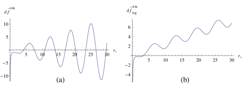
Finally, introducing the log-gravity, a suggested solution as a logarithmic partner of $\delta\tilde{f}_{ml}$ takes the form [31] of

$$\delta\tilde{F}^{\rm 4th}_{\rm log}(r_{*})=e^{-i\omega t}\delta\tilde{f}^{\rm 4th}_{\rm log}(r_{*}),$$ (66)

where

$\displaystyle\delta\tilde{f}^{\rm 4th}_{\rm log}(r_{*})=\left.\frac{\partial}{\partial m^{2}}\{\sqrt{r_{*}}Y_{\nu}(r_{*})\}\right|_{m^{2}=0}$
$\displaystyle=\frac{v\sqrt{r_{*}}}{3}\left[\ \cot[3\pi/2]\left(J_{3/2}(r_{*})\ln(r_{*}/2)-\Big{(}\frac{r_{*}}{2}\Big{)}^{3/2}\sum^{\infty}_{k=0}(-1)^{k}\frac{\psi(5/2+k)}{\Gamma(5/2+k)}\frac{(\frac{1}{4}r^{2}_{*})^{k}}{k!}-\pi Y_{3/2}(r_{*})\right)\right.$
$\displaystyle~{}~{}~{}~{}+\csc[3\pi/2]\left(J_{-3/2}(r_{*})\ln(r_{*}/2)-\Big{(}\frac{r_{*}}{2}\Big{)}^{-3/2}\sum^{\infty}_{k=0}(-1)^{k}\frac{\psi(-1/2+k)}{\Gamma(-1/2+k)}\frac{(\frac{1}{4}r^{2}_{*})^{k}}{k!}\right)-\pi J_{3/2}(r_{*})\Bigg{]}$
$\displaystyle=\frac{v}{3}\left(\frac{3a}{\sqrt{2\pi}}r_{*}-\pi\sqrt{r_{*}}J_{3/2}(r_{*})-\ln(r_{*}/2)Y_{3/2}(r_{*})\right)$ (67)

with $a=0.616108$. Fig. (3b) indicates $\delta\tilde{f}^{\rm 4th}_{\rm log}(r_{*})$ is singular at $r_{*}=0$. To show it explicitly, one finds a series expansion of $\tilde{f}^{\rm 4th}_{\rm log}(r_{*})$ as

$\displaystyle\tilde{f}^{\rm 4th}_{\rm log}(r_{*})$ $\displaystyle\simeq$ $\displaystyle v\sqrt{\frac{2}{\pi}}\left[\left(\frac{1}{3r_{*}}+\frac{1}{6}r_{*}-\frac{1}{24}r^{3}_{*}+\frac{1}{432}r^{5}_{*}\right)\ln(r_{*}/2)+\left(\frac{a}{2}r_{*}-\frac{\pi}{9}r^{2}_{*}+\frac{\pi}{90}r^{4}_{*}\right)+\cdots\right].$

Here we note that the first term in $\ln(r_{*}/2)$ shows a singular behavior as $r_{*}\to 0$, while the remaining terms makes a finite graph as an oscillatory increasing function for large $r_{*}$.

5 Discussions

We have studied the critical gravity in AdS2 spacetimes, which was obtained from the topologically massive gravity in three dimensions by using the Kaluza-Klein dimensional reduction. We have performed the perturbation analysis around the AdS2, which corresponds to the near-horizon geometry of the extremal BTZ black hole obtained from the topological massive gravity with identification upon uplifting three dimensions. A physically massive scalar mode $\delta F$ satisfies the second-order differential equation away from the critical point of $K=l$, while it satisfies the fourth-order equation at the critical point. At the critical point, the 2DTMGΞ› turns out to be the 2D dilaton gravity including the Maxwell field obtained from the 3D Einstein gravity, which shows implicitly that there are no propagating modes.

Based on that the critical gravity has a new field in AdS spacetimes, we have exactly solved the fourth-order equation, and compared it with the log-gravity ansatz in two dimensions. The critical gravity is described by $\delta f^{\rm 4th}$ (52) precisely, which, however, it becomes divergent linearly ($r\to\infty$) as the infinity of $r_{*}=0~{}(r=\infty)$ is approached. This means that the solution to the fourth-order equation is not a precisely normalizable function and thus, it requires to introduce an appropriate boundary condition which accommodates a linear divergence.

More importantly, it has turned out that the critical gravity could not be described by the massless scalar $\delta f_{\rm ml}$ and its logarithmic partner $\delta f^{\rm 4th}_{\rm log}$ (58), which approaches zero as $r_{*}\to 0$. This is so because $\delta f^{\rm 4th}_{\rm log}$ unlikely satisfies the fourth-order equation.

Finally, we would like to comment that the linearized higher dimensional critical gravities were widely investigated in the AdS spacetimes [26] but the non-unitarity issue of the log-gravity is not still resolved, indicating that any log-gravity suffers from the ghost problem. Furthermore, the critical gravity on the Schwarzschild-AdS black hole has suffered from the ghost problem when the cross term $E_{\rm cross}$ is non-vanishing [32].


Acknowledgements

Y.S. Myung and Y.-W. Kim were supported by Basic Science Research Program through the National Research Foundation (KRF) of Korea funded by the Ministry of Education, Science and Technology (2010-0028080). Y.-J. Park was supported by World Class University program funded by the Ministry of Education, Science and Technology through the National Research Foundation of Korea(No. R31-20002). Y. S. Myung and Y.-J. Park were also supported by the National Research Foundation of Korea (NRF) grant funded by the Korea government (MEST) through the Center for Quantum Spacetime (CQUeST) of Sogang University with grant number 2005-0049409.

References

  • [1] S. Deser, R. Jackiw and S. Templeton, Annals Phys.  140, 372 (1982) [Erratum-ibid.  185, 406 (1988)] [Annals Phys.  185, 406 (1988)] [Annals Phys.  281, 409 (2000)].
  • [2] S. Deser, β€œCosmological Topological Supergravity” in Quantum Theory of Gravity, ed. S.M. Christensen, Adam Hilger, London (1984).
  • [3] W. Li, W. Song and A. Strominger, JHEP 0804, 082 (2008) [arXiv:0801.4566 [hep-th]].
  • [4] S. Deser and B. Tekin, Phys. Rev. Lett.  89, 101101 (2002) [arXiv:hep-th/0205318]; S. Deser and B. Tekin, Phys. Rev.  D 67, 084009 (2003) [arXiv:hep-th/0212292].
  • [5] S. Carlip, S. Deser, A. Waldron and D. K. Wise, Class. Quant. Grav.  26, 075008 (2009) [arXiv:0803.3998 [hep-th]].
  • [6] D. Grumiller and N. Johansson, JHEP 0807, 134 (2008) [arXiv:0805.2610 [hep-th]].
  • [7] G. Giribet, M. Kleban and M. Porrati, JHEP 0810, 045 (2008) [arXiv:0807.4703 [hep-th]].
  • [8] M. I. Park, JHEP 0809, 084 (2008) [arXiv:0805.4328 [hep-th]].
  • [9] D. Grumiller, R. Jackiw and N. Johansson, arXiv:0806.4185 [hep-th].
  • [10] S. Carlip, S. Deser, A. Waldron and D. K. Wise, Phys. Lett.  B 666, 272 (2008) [arXiv:0807.0486 [hep-th]].
  • [11] S. Carlip, JHEP 0810, 078 (2008) [arXiv:0807.4152 [hep-th]].
  • [12] A. Strominger, arXiv:0808.0506 [hep-th].
  • [13] G. Guralnik, A. Iorio, R. Jackiw and S. Y. Pi, Annals Phys.  308, 222 (2003) [arXiv:hep-th/0305117].
  • [14] D. Grumiller and W. Kummer, Annals Phys. 308, 211 (2003) [arXiv:hep-th/0306036].
  • [15] E. A. Bergshoeff, O. Hohm and P. K. Townsend, Phys. Rev. Lett.  102, 201301 (2009) [arXiv:0901.1766 [hep-th]].
  • [16] B. Sahoo and A. Sen, JHEP 0607, 008 (2006) [arXiv:hep-th/0601228].
  • [17] M. Alishahiha, R. Fareghbal and A. E. Mosaffa, JHEP 0901, 069 (2009) [arXiv:0812.0453 [hep-th]].
  • [18] M. Banados, C. Teitelboim and J. Zanelli, Phys. Rev. Lett.  69, 1849 (1992) [arXiv:hep-th/9204099].
  • [19] Y. W. Kim, Y. S. Myung and Y. J. Park, Eur. Phys. J.  C 67, 533 (2010) [arXiv:0901.4390 [hep-th]].
  • [20] I. Sachs and S. N. Solodukhin, JHEP 0808, 003 (2008) [arXiv:0806.1788 [hep-th]].
  • [21] M. A. I. Flohr, Int. J. Mod. Phys.  A 11, 4147 (1996) [arXiv:hep-th/9509166].
  • [22] I. I. Kogan and A. Lewis, Phys. Lett.  B 431, 77 (1998) [arXiv:hep-th/9802102].
  • [23] A. M. Ghezelbash, M. Khorrami and A. Aghamohammadi, Int. J. Mod. Phys.  A 14, 2581 (1999) [arXiv:hep-th/9807034].
  • [24] Y. S. Myung and H. W. Lee, JHEP 9910, 009 (1999) [arXiv:hep-th/9904056].
  • [25] Y. S. Myung, Phys. Lett.  B 670, 220 (2008) [arXiv:0808.1942 [hep-th]].
  • [26] H. Lu and C. N. Pope, arXiv:1101.1971 [hep-th]; S. Deser, H. Liu, H. Lu, C. N. Pope, T. C. Sisman and B. Tekin, Phys. Rev.  D 83, 061502 (2011) [arXiv:1101.4009 [hep-th]]; M. Alishahiha and R. Fareghbal, Phys. Rev.  D 83, 084052 (2011) [arXiv:1101.5891 [hep-th]]; E. A. Bergshoeff, O. Hohm, J. Rosseel and P. K. Townsend, arXiv:1102.4091 [hep-th]; M. Porrati and M. M. Roberts, arXiv:1104.0674 [hep-th].
  • [27] Y. S. Myung, Y. W. Kim and Y. J. Park, JHEP 0906, 043 (2009) [arXiv:0901.2141 [hep-th]].
  • [28] Y. S. Myung, Y. W. Kim, T. Moon and Y. J. Park, arXiv:1105.4205 [hep-th].
  • [29] V. Balasubramanian, J. de Boer, M. M. Sheikh-Jabbari and J. Simon, JHEP 1002, 017 (2010) [arXiv:0906.3272 [hep-th]].
  • [30] M. Spradlin and A. Strominger, JHEP 9911, 021 (1999) [arXiv:hep-th/9904143].
  • [31] M. Abramowitz and I. Stegan, Handbook of Matematical Functions (Academic Press, New York, 1966).
  • [32] H. Liu, H. Lu and M. Luo, arXiv:1104.2623 [hep-th].