Beta processes, stick-breaking, and power laws

Abstract

The beta-Bernoulli process provides a Bayesian nonparametric prior for models involving collections of binary-valued features. A draw from the beta process yields an infinite collection of probabilities in the unit interval, and a draw from the Bernoulli process turns these into binary-valued features. Recent work has provided stick-breaking representations for the beta process analogous to the well-known stick-breaking representation for the Dirichlet process. We derive one such stick-breaking representation directly from the characterization of the beta process as a completely random measure. This approach motivates a three-parameter generalization of the beta process, and we study the power laws that can be obtained from this generalized beta process. We present a posterior inference algorithm for the beta-Bernoulli process that exploits the stick-breaking representation, and we present experimental results for a discrete factor-analysis model.

1 Introduction

Large data sets are often heterogeneous, arising as amalgams from underlying sub-populations. The analysis of large data sets thus often involves some form of stratification in which groupings are identified that are more homogeneous than the original data. While this can sometimes be done on the basis of explicit covariates, it is also commonly the case that the groupings are captured via discrete latent variables that are to be inferred as part of the analysis. Within a Bayesian framework, there are two widely employed modeling motifs for problems of this kind. The first is the Dirichlet-multinomial motif, which is based on the assumption that there are $K$ “clusters” that are assumed to be mutually exclusive and exhaustive, such that allocations of data to clusters can be modeled via a multinomial random variable whose parameter vector is drawn from a Dirichlet distribution. A second motif is the beta-Bernoulli motif, where a collection of $K$ binary “features” are used to describe the data, and where each feature is modeled as a Bernoulli random variable whose parameter is obtained from a beta distibution. The latter motif can be converted to the former in principle—we can view particular patterns of ones and zeros as defining a cluster, thus obtaining $M=2^{K}$ clusters in total. But in practice models based on the Dirichlet-multinomial motif typically require $O(M)$ additional parameters in the likelihood, whereas those based on the beta-Bernoulli motif typically require only $O(K)$ additional parameters. Thus, if the combinatorial structure encoded by the binary features captures real structure in the data, then the beta-Bernoulli motif can make more efficient usage of its parameters.

The Dirichlet-multinomial motif can be extended to a stochastic process known as the Dirichlet process. A draw from a Dirichlet process is a random probability measure that can be represented as follows (McCloskey, 1965; Patil and Taillie, 1977; Ferguson, 1973; Sethuraman, 1994):

$$G=\sum_{i=1}^{\infty}\pi_{i}\delta_{\psi_{i}},$$ (1)

where $\delta_{\psi_{i}}$ represents an atomic measure at location $\psi_{i}$, where both the $\{\pi_{i}\}$ and the $\{\psi_{i}\}$ are random, and where the $\{\pi_{i}\}$ are nonnegative and sum to one (with probability one). Conditioning on $G$ and drawing $N$ values independently from $G$ yields a collection of $K$ distinct values, where $K\leq N$ is random and grows (in expectation) at rate $O(\log N)$. Treating these distinct values as indices of clusters, we obtain a model in which the number of clusters is random and subject to posterior inference.

A great deal is known about the Dirichlet process—there are direct connections between properties of $G$ as a random measure (e.g., it can be obtained from a Poisson point process), properties of the sequence of values $\{\pi_{i}\}$ (they can be obtained from a “stick-breaking process”), and properties of the collection of distinct values obtained by sampling from $G$ (they are characterized by a stochastic process known as the Chinese restaurant process). These connections have helped to place the Dirichlet process at the center of Bayesian nonparametrics, driving the development of a wide variety of inference algorithms for models based on Dirichlet process priors and suggesting a range of generalizations (e.g. MacEachern, 1999; Ishwaran and James, 2001; Walker, 2007; Kalli et al., 2009).

It is also possible to extend the beta-Bernoulli motif to a Bayesian nonparametric framework, and there is a growing literature on this topic. The underlying stochastic process is the beta process, which is an instance of a family of random measures known as completely random measures (Kingman, 1967). The beta process was first studied in the context of survival analysis by Hjort (1990), where the focus is on modeling hazard functions via the random cumulative distribution function obtained by integrating the beta process. Thibaux and Jordan (2007) focused instead on the beta process realization itself, which can be represented as

$$G=\sum_{i=1}^{\infty}q_{i}\delta_{\psi_{i}},$$

where both the $q_{i}$ and the $\psi_{i}$ are random and where the $q_{i}$ are contained in the interval $(0,1)$. This random measure can be viewed as furnishing an infinite collection of coins, which, when tossed repeatedly, yield a binary featural description of a set of entities in which the number of features with non-zero values is random. Thus, the resulting beta-Bernoulli process can be viewed as an infinite-dimensional version of the beta-Bernoulli motif. Indeed, Thibaux and Jordan (2007) showed that by integrating out the random $q_{i}$ and $\psi_{i}$ one obtains—by analogy to the derivation of the Chinese restaurant process from the Dirichlet process—a combinatorial stochastic process known as the Indian buffet process, previously studied by Griffiths and Ghahramani (2006), who derived it via a limiting process involving random binary matrices obtained by sampling finite collections of beta-Bernoulli variables.

Stick-breaking representations of the Dirichlet process have been particularly important both for algorithmic development and for exploring generalizations of the Dirichlet process. These representations yield explicit recursive formulas for obtaining the weights $\{\pi_{i}\}$ in Eq. (1). In the case of the beta process, explicit non-recursive representations can be obtained for the weights $\{q_{i}\}$, based on size-biased sampling (Thibaux and Jordan, 2007) and inverse Lévy measure (Wolpert and Ickstadt, 2004; Teh et al., 2007). Recent work has also yielded recursive constructions that are more closely related to the stick-breaking representation of the Dirichlet process (Teh et al., 2007; Paisley et al., 2010).

Stick-breaking representations of the Dirichlet process permit ready generalizations to stochastic processes that yield power-law behavior (which the Dirichlet process does not), notably the Pitman-Yor process (Ishwaran and James, 2001; Pitman, 2006). Power-law generalizations of the beta process have also been studied (Teh and Görür, 2009) and stick-breaking-like representations derived. These latter representations are, however, based on the non-recursive sized-biased sampling and inverse-Lévy methods rather than the recursive representations of Teh et al. (2007) and Paisley et al. (2010).

Teh et al. (2007) and Paisley et al. (2010) derived their stick-breaking representations of the beta process as limiting processes, making use of the derivation of the Indian buffet process by Griffiths and Ghahramani (2006) as a limit of finite-dimensional random matrices. In the current paper we show how to derive stick-breaking for the beta process directly from the underlying random measure. This approach not only has the advantage of conceptual clarity (our derivation is elementary), but it also permits a unified perspective on various generalizations of the beta process that yield power-law behavior. We show in particular that it yields a power-law generalization of the stick-breaking representation of Paisley et al. (2010).

To illustrate our results in the context of a concrete application, we study a discrete factor analysis model previously considered by Griffiths and Ghahramani (2006) and Paisley et al. (2010). The model is of the form

$$X=Z\Phi+E,$$ (2)

where $X\in\mathbb{R}^{N\times P}$ is the data and $E\in\mathbb{R}^{N\times P}$ is an error matrix. The matrix $\Phi\in\mathbb{R}^{K\times P}$ is a matrix of factors, and $Z\in\mathbb{R}^{N\times K}$ is a binary matrix of factor loadings. The dimension $K$ is infinite, and thus the rows of $\Phi$ comprise an infinite collection of factors. The matrix $Z$ is obtained via a draw from a beta-Bernoulli process; its $n$th row is an infinite binary vector of features (i.e., factor loadings) encoding which of the infinite collection of factors are used in modeling the $n$th data point.

The remainder of the paper is organized as follows. We introduce the beta process, and its conjugate measure the Bernoulli process, in Section 2. In order to consider stick-breaking and power law behavior in the beta-Bernoulli framework, we first review stick-breaking for the Dirichlet process in Section 3 and power laws in clustering models in Section 4.1. We consider potential power laws that might exist in featural models in Section 4.2. Our main theoretical results come in the following two sections. First, in Section 5, we provide a proof that the stick-breaking representation of Paisley et al. (2010), expanded to include a third parameter, holds for a three-parameter extension of the beta process. Our proof takes a measure-theoretic approach based on a Poisson process. We then make use of the Poisson process framework to establish asymptotic power laws, with exact constants, for the three-parameter beta process in Section 6.1. We also show, in Section 6.2, that there are aspects of the beta-Bernoulli framework that cannot exhibit a power law. We illustrate the asymptotic power laws on a simulated data set in Section 7. We present experimental results in Section 8, and we present an MCMC algorithm for posterior inference in Appendix A.

2 The beta process and the Bernoulli process

The beta process and the Bernoulli process are instances of the general family of random measures known as completely random measures (Kingman, 1967). A completely random measure $H$ on a probability space $(\Psi,{\cal S})$ is a random measure such that, for any disjoint measurable sets $A_{1},\ldots,A_{n}\in{\cal S}$, the random variables $H(A_{1}),\ldots,H(A_{n})$ are independent.

Completely random measures can be obtained from an underlying Poisson point process. Let $\nu(d\psi,du)$ denote a $\sigma$-finite measure on the product space $\Psi\times\mathbb{R}$. Draw a realization from a Poisson point process with rate measure $\nu(d\psi,du)$. This yields a set of points $\Pi=\{(\psi_{i},U_{i})\}_{i}$, where the index $i$ may range over a countable infinity. Finally, construct a random measure as follows:

$$B=\sum_{i=1}^{\infty}U_{i}\delta_{\psi_{i}},$$ (3)

where $\delta_{\psi_{i}}$ denotes an atom at $\psi_{i}$. This discrete random measure is such that for any measurable set $T\in{\cal S}$,

$$B(T)=\sum_{i:\psi_{i}\in T}U_{i}.$$

That $B$ is completely random follows from the Poisson point process construction.

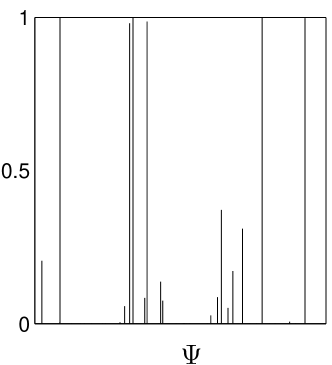
In addition to the representation obtained from a Poisson process, completely random measures may include a deterministic measure and a set of atoms at fixed locations. The component of the completely random measure generated from a Poisson point process as described above is called the ordinary component. As shown by Kingman (1967), completely random measures are essentially characterized by this representation. An example is shown in Figure 1.

Figure 1: The gray surface illustrates the rate density in Eq. (4) corresponding to the beta process. The base measure $B_{0}$ is taken to be uniform on $\Psi$. The non-zero endpoints of the line segments plotted below the surface are a particular realization of the Poisson process, and the line segments themselves represent a realization of the beta process.

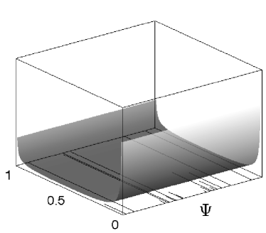
The beta process, denoted $B\sim\textrm{BP}(\theta,B_{0})$, is an example of a completely random measure. As long as the base measure $B_{0}$ is continuous, which is our assumption here, $B$ has only an ordinary component with rate measure

$$\nu_{\textrm{BP}}(d\psi,du)=\theta(\psi)u^{-1}(1-u)^{\theta(\psi)-1}\;du\;B_{0}(d\psi),\quad\psi\in\Psi,u\in[0,1],$$ (4)

where $\theta$ is a positive function on $\Psi$. The function $\theta$ is called the concentration function (Hjort, 1990). In the remainder we follow Thibaux and Jordan (2007) in taking $\theta$ to be a real-valued constant and refer to it as the concentration parameter. We assume $B_{0}$ is nonnegative and fixed. The total mass of $B_{0}$, $\gamma:=B_{0}(\Psi)$, is called the mass parameter. We assume $\gamma$ is strictly positive and finite. The density in Eq. (4), with the choice of $B_{0}$ uniform over $[0,1]$, is illustrated in Figure 1.

Figure 2: Upper left: A draw $B$ from the beta process. Lower left: 50 draws from the Bernoulli process $BeP(B)$. The vertical axis indexes the draw number among the 50 exchangeable draws. A point indicates a one at the corresponding location on the horizontal axis, $\psi\in\Psi$. Right: We can form a matrix from the lower left plot by including only those $\psi$ values with a non-zero number of Bernoulli successes among the 50 draws from the Bernoulli process. Then, the number of columns $K$ is the number of such $\psi$, and the number of rows $N$ is the number of draws made. A black square indicates a one at the corresponding matrix position; a white square indicates a zero.

The beta process can be viewed as providing an infinite collection of coin-tossing probabilities. Tossing these coins corresponds to a draw from the Bernoulli process, yielding an infinite binary vector that we will treat as a latent feature vector.

More formally, a Bernoulli process $Y\sim BeP(B)$ is a completely random measure with potentially both fixed atomic and ordinary components. In defining the Bernoulli process we consider only the case in which $B$ is discrete, i.e., of the form in Eq. (3), though not necessarily a beta process draw or even random for the moment. Then $Y$ has only a fixed atomic component and has the form

$$Y=\sum_{i=1}^{\infty}b_{i}\delta_{\psi_{i}},$$ (5)

where $b_{i}\sim\textrm{Bern}(u_{i})$ for $u_{i}$ the corresponding atomic mass in the measure $B$. We can see that $\mathbb{E}(Y|B)=B(\Psi)$ from the mean of the Bernoulli distribution, so the number of non-zero points in any realization of the Bernoulli process is finite when $B$ is a finite measure.

We can link the beta process and $N$ Bernoulli process draws to generate a random feature matrix $Z$. To that end, first draw $B\sim\textrm{BP}(\theta,B_{0})$ for fixed hyperparameters $\theta$ and $B_{0}$ and then draw $Y_{n}\stackrel{{\scriptstyle iid}}{{\sim}}\textrm{BeP}(B)$ for $n\in\{1,\ldots,N\}$. Note that since $B$ is discrete, each $Y_{n}$ will be discrete as in Eq. (5), with point masses only at the atoms $\{\psi_{i}\}$ of the beta process $B$. Note also that $\mathbb{E}B(\Psi)=\gamma<\infty$, so $B$ is a finite measure, and it follows that the number of non-zero point masses in any draw $Y_{n}$ from the Bernoulli process will be finite. Therefore, the total number of non-zero point masses $K$ across $N$ such Bernoulli process draws is finite.

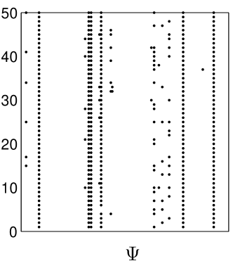
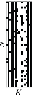
Now reorder the $\{\psi_{i}\}$ so that the first $K$ are exactly those locations where some Bernoulli process in $\{Y_{n}\}_{n=1}^{N}$ has a non-zero point mass. We can form a matrix $Z\in\{0,1\}^{N\times K}$ as a function of the $\{Y_{n}\}_{n=1}^{N}$ by letting the $(n,k)$ entry equal one when $Y_{n}$ has a non-zero point mass at $\psi_{k}$ and zero otherwise. If we wish to think of $Z$ as having an infinite number of columns, the remaining columns represent the point masses of the $\{Y_{n}\}_{n=1}^{N}$ at $\{\psi_{k}\}_{k>K}$, which we know to be zero by construction. We refer to the overall procedure of drawing $Z$ according to, first, a beta process and then repeated Bernoulli process draws in this way as a beta-Bernoulli process, and we write $Z\sim\textrm{BP-BeP}(N,\gamma,\theta)$. Note that we have implicitly integrated out the $\{\psi_{k}\}$, and the distribution of the matrix $Z$ depends on $B_{0}$ only through its total mass, $\gamma$. As shown by Thibaux and Jordan (2007), this process yields the same distribution on row-exchangeable, infinite-column matrices as the Indian buffet process (Griffiths and Ghahramani, 2006), which describes a stochastic process directly on (equivalence classes of) binary matrices. That is, the Indian buffet process is obtained as an exchangeable distribution on binary matrices when the underlying beta process measure is integrated out. This result is analogous to the derivation of the Chinese restaurant process as the exchangeable distribution on partitions obtained when the underlying Dirichlet process is integrated out. The beta-Bernoulli process is illustrated in Figure 2.

3 Stick-breaking for the Dirichlet process

Figure 3: A stick-breaking process starts with the unit interval (far left). First, a random fraction $V_{1}$ of the unit interval is broken off; the remaining stick has length $1-V_{1}$ (middle left). Next, a random fraction $V_{2}$ of the remaining stick is broken off, i.e., a fragment of size $V_{2}(1-V_{1})$; the remaining stick has length $(1-V_{1})(1-V_{2})$. This process proceeds recursively and generates stick fragments $V_{1},V_{2}(1-V_{1}),\ldots,V_{i}\prod_{j<i}(1-V_{j}),\ldots$. These fragments form a random partition of the unit interval (far right).

The stick-breaking representation of the Dirichlet process (McCloskey, 1965; Patil and Taillie, 1977; Sethuraman, 1994) provides a simple recursive procedure for obtaining the weights $\{\pi_{i}\}$ in Eq. (1). This procedure provides an explicit representation of a draw $G$ from the Dirichlet process, one which can be usefully instantiated and updated in posterior inference algorithms (Ishwaran and James, 2001; Blei and Jordan, 2006). We begin this section by reviewing this stick-breaking construction as well as some of the extensions to this construction that yield power-law behavior. We then turn to a consideration of stick-breaking and power laws in the setting of the beta process.

Stick-breaking is the process of recursively breaking off random fractions of the unit interval. In particular, let $V_{1},V_{2},\ldots$ be some countable sequence of random variables, each with range $[0,1]$. Each $V_{i}$ represents the fraction of the remaining stick to break off at step $i$. Thus, the first stick length generated by the stick-breaking process is $V_{1}$. At this point, a fragment of length $1-V_{1}$ of the original stick remains. Breaking off $V_{2}$ fraction of the remaining stick yields a second stick fragment of $V_{2}(1-V_{1})$. This process iterates such that the stick length broken off at step $i$ is $V_{i}\prod_{j<i}(1-V_{j})$. The stick-breaking recursion is illustrated in Figure 3.

The Dirichlet process arises from the special case in which the $V_{i}$ are independent draws from the $\textrm{Beta}(1,\theta)$ distribution (McCloskey, 1965; Patil and Taillie, 1977; Sethuraman, 1994). Thus we have the following representation of a draw $G\sim\textrm{DP}(\theta,G_{0})$:

$$G = \sum_{i=1}^{\infty}\left[V_{i}\prod_{j=1}^{i-1}(1-V_{j})\right]\delta_{\psi_{i}}$$

$$V_{i} \stackrel{{\scriptstyle iid}}{{\sim}} \textrm{Beta}(1,\theta)$$

$$\psi_{i} \stackrel{{\scriptstyle iid}}{{\sim}} G_{0},$$ (6)

where $G_{0}$ is referred to as the base measure and $\theta$ is referred to as the concentration parameter.

4 Power law behavior

Consider the process of sampling a random measure $G$ from a Dirichlet process and subsequently drawing independently $N$ times from $G$. The number of unique atoms sampled according to this process will grow as a function of $N$. The growth associated with the Dirichlet process is relatively slow, however, and when the Dirichlet process is used as a prior in a clustering model one does not obtain the heavy-tailed behavior commonly referred to as a “power law.” In this section we first provide a brief exposition of the different kinds of power law that we might wish to obtain in a clustering model and discuss how these laws can be obtained via an extension of the stick-breaking representation. We then discuss analogous laws for featural models.

4.1 Power laws in clustering models

First, we establish some notation. Given a number $N$ of draws from a discrete random probability measure $G$ (where $G$ is not necessarily a draw from the Dirichlet process), let $(N_{1},N_{2},\ldots)$ denote the sequence of counts associated with the unique values obtained among the $N$ draws, where we view these unique values as “clusters.” Let

$$K_{N,j}=\sum_{i=1}^{\infty}\mathbbm{1}(N_{i}=j),$$ (7)

and let

$$K_{N}=\sum_{i=1}^{\infty}\mathbbm{1}(N_{i}>0).$$ (8)

That is, $K_{N,j}$ is the number of clusters that are drawn exactly $j$ times, and $K_{N}$ is the total number of clusters.

There are two types of power-law behavior that a clustering model might exhibit. First, there is the type of power law behavior reminiscent of Heaps’ law (Heaps, 1978; Gnedin et al., 2007):

$$K_{N}\stackrel{{\scriptstyle a.s.}}{{\sim}}cN^{a},\quad N\rightarrow\infty$$ (9)

for some constants $c>0,a\in(0,1)$. Here, $\sim$ means that the limit of the ratio of the left-hand and right-hand side, when they are both real-valued and non-random, is one as the number of data points $N$ grows large. We denote a power law in the form of Eq. (9) as Type I. Second, there is the type of power law behavior reminiscent of Zipf’s law (Zipf, 1949; Gnedin et al., 2007):

$$K_{N,j}\stackrel{{\scriptstyle a.s.}}{{\sim}}\frac{a\Gamma(j-a)}{j!\Gamma(1-a)}cN^{a}\quad N\rightarrow\infty$$ (10)

again for some constants $c>0,a\in(0,1)$. We refer to the power law in Eq. (10) as Type II.

Sometimes in the case of Eq. (10), we are interested in the behavior in $j$; therefore we recall $j!=\Gamma(j+1)$ and note the following fact about the $\Gamma$-function ratio in Eq. (10) (cf. Tricomi and Erdélyi, 1951):

$$\frac{\Gamma(j-a)}{\Gamma(j+1)}\sim j^{-1-a}\quad j\rightarrow\infty$$ (11)

Again, we see behavior in the form of a power law at work.

Power-law behavior of Types I and II (and equivalent formulations; see Gnedin et al., 2007) has been observed in a variety of real-world clustering problems including, but not limited to: the number of species per plant genus, the in-degree or out-degree of a graph constructed from hyperlinks on the Internet, the number of people in cities, the number of words in documents, the number of papers published by scientists, and the amount each person earns in income (Mitzenmacher, 2004; Goldwater et al., 2006). Bayesians modeling these situations will prefer a prior that reflects this distributional attribute.

While the Dirichlet process exhibits neither type of power-law behavior, the Pitman-Yor process yields both kinds of power law (Pitman and Yor, 1997; Goldwater et al., 2006) though we note that in this case $c$ is a random variable (still with no dependence on $N$ or $j$). The Pitman-Yor process, denoted $G\sim\textrm{PY}(\theta,\alpha,G_{0})$, is defined via the following stick-breaking representation:

$$G = \sum_{i=1}^{\infty}\left[V_{i}\prod_{j=1}^{i-1}(1-V_{j})\right]\delta_{\psi_{i}}$$

$$V_{i} \stackrel{{\scriptstyle indep}}{{\sim}} \textrm{Beta}(1-\alpha,\theta+i\alpha)$$

$$\psi_{i} \stackrel{{\scriptstyle iid}}{{\sim}} G_{0},$$ (12)

where $\alpha$ is known as a discount parameter. The case $\alpha=0$ returns the Dirichlet process (cf. Eq. (6)).

Note that in both the Dirichlet process and Pitman-Yor process, the weights $\{V_{i}\prod_{j=1}^{i-1}(1-V_{j})\}$ are the weights of the process in size-biased order (Pitman, 2006). In the Pitman-Yor case, the $\{V_{i}\}$ are no longer identically distributed.

4.2 Power laws in featural models

The beta-Bernoulli process provides a specific kind of feature-based representation of entities. In this section we study general featural models and consider the power laws that might arise for such models.

In the clustering framework, we considered $N$ draws from a process that put exactly one mass of size one on some value in $\Psi$ and mass zero elsewhere. In the featural framework we consider $N$ draws from a process that places some non-negative integer number of masses, each of size one, on an almost surely finite set of values in $\Psi$ and mass zero elsewhere. As $N_{i}$ was the sum of masses at a point labeled $\psi_{i}\in\Psi$ in the clustering framework, so do we now let $N_{i}$ be the sum of masses at a point labeled $\psi_{i}\in\Psi$. We use the same notation as in Section 4.1, but now we note that the counts $N_{i}$ no longer sum to $N$ in general.

In the case of featural models, we can still talk about Type I and II power laws, both of which have the same interpretation as in the case of clustering models. In the featural case, however, it is also possible to consider a third type of power law. If we let $k_{n}$ denote the number of features present in the $n$th draw, we say that $k_{n}$ shows power law behavior if

$$\mathbb{P}(k_{n}>M)\sim cM^{-a}$$

for positive constants $c$ and $a$. We call this last type of power law Type III.

5 Stick-breaking for the beta process

The weights $\{q_{i}\}$ for the beta process can be derived by a variety of procedures, including size-biased sampling (Thibaux and Jordan, 2007) and inverse Lévy measure (Wolpert and Ickstadt, 2004; Teh et al., 2007). The procedures that are closest in spirit to the stick-breaking representation for the Dirichlet process are those due to Paisley et al. (2010) and Teh et al. (2007). Our point of departure is the former, which has the following form:

$$B = \sum_{i=1}^{\infty}\sum_{j=1}^{C_{i}}V_{i,j}^{(i)}\prod_{l=1}^{i-1}(1-V_{i,j}^{(l)})\delta_{\psi_{i,j}}$$

$$C_{i} \stackrel{{\scriptstyle iid}}{{\sim}} \textrm{Pois}(\gamma)$$

$$V_{i,j}^{(l)} \stackrel{{\scriptstyle iid}}{{\sim}} \textrm{Beta}(1,\theta)$$

$$\psi_{i,j} \stackrel{{\scriptstyle iid}}{{\sim}} \frac{1}{\gamma}B_{0}.$$ (13)

This representation is analogous to the stick-breaking representation of the Dirichlet process in that it represents a draw from the beta process as a sum over independently drawn atoms, with the weights obtained by a recursive procedure. However, it is worth noting that for every $(i,j)$ tuple subscript for $V_{i,j}^{(l)}$, a different stick exists and is broken across the superscript $l$. Thus, there are no special additive properties across weights in the sum in Eq. (13); by contrast, the weights in Eq. (12) sum to one almost surely.

The generalization of the one-parameter Dirichlet process to the two-parameter Pitman-Yor process suggests that we might consider generalizing the stick-breaking representation of the beta process in Eq. (13) as follows:

$$B = \sum_{i=1}^{\infty}\sum_{j=1}^{C_{i}}V_{i,j}^{(i)}\prod_{l=1}^{i-1}(1-V_{i,j}^{(l)})\delta_{\psi_{i,j}}$$

$$C_{i} \stackrel{{\scriptstyle iid}}{{\sim}} \textrm{Pois}(\gamma)$$

$$V_{i,j}^{(l)} \stackrel{{\scriptstyle indep}}{{\sim}} \textrm{Beta}(1-\alpha,\theta+i\alpha)$$

$$\psi_{i,j} \stackrel{{\scriptstyle iid}}{{\sim}} \frac{1}{\gamma}B_{0}.$$ (14)

In Section 6 we will show that introducing the additional parameter $\alpha$ indeed yields Type I and II power law behavior (but not Type III).

In the remainder of this section we present a proof that these stick-breaking representations arise from the beta process. In contradistinction to the proof of Eq. (13) by Paisley et al. (2010), which used a limiting process defined on sequences of finite binary matrices, our approach makes a direct connection to the Poisson process characterization of the beta process. Our proof has several virtues: (1) it relies on no asymptotic arguments and instead comes entirely from the Poisson process representation; (2) it is, as a result, simpler and shorter; and (3) it demonstrates clearly the ease of incorporating a third parameter analogous to the discount parameter of the Pitman-Yor process and thereby provides a strong motivation for the extended stick-breaking representation in Eq. (14).

Aiming toward the general stick-breaking representation in Eq. (14), we begin by defining a three-parameter generalization of the beta process. We say that $B\sim\textrm{BP}(\theta,\alpha,B_{0})$, where we call $\alpha$ a discount parameter, if, for $\psi\in\Psi,u\in[0,1])$, we have

$$\nu_{\textrm{BP}}(d\psi,du)=\frac{\Gamma(1+\theta)}{\Gamma(1-\alpha)\Gamma(\theta+\alpha)}u^{-1-\alpha}(1-u)^{\theta+\alpha-1}\;du\;B_{0}(d\psi).$$ (15)

It is straightforward to show that this three-parameter density has similar properties to that of the two-parameter beta process. For instance, choosing $\alpha\in(0,1)$ and $\theta>-\alpha$ is necessary for the beta process to have finite total mass almost surely; in this case,

$$\int_{\Psi\times\mathbb{R}_{+}}u\;\nu_{\textrm{BP}}(d\psi,du)=\frac{\Gamma(1-\alpha)\Gamma(\theta+\alpha)}{\Gamma(1+\theta)}<\infty.$$ (16)

We now turn to the main result of this section.

Proposition 1.

$B$ can be represented according to the process described in Eq. (14) if and only if $B\sim\textrm{BP}(\theta,\alpha,B_{0})$.

Proof.

First note that the points in the set

$$P_{1}:=\left\{(\psi_{1,1},V_{1,1}^{(1)}),(\psi_{1,2},V_{1,2}^{(1)}),\ldots,(\psi_{1,C_{1}},V_{1,C_{1}}^{(1)})\right\}$$

are by construction independent and identically distributed conditioned on $C_{1}$. Since $C_{1}$ is Poisson-distributed, $P_{1}$ is a Poisson point process. The same logic gives that in general, for

$$P_{i}:=\left\{\left(\psi_{i,1},V_{i,1}^{(i)}\prod_{l=1}^{i-1}(1-V_{i,1}^{(l)})\right),\ldots,\left(\psi_{i,C_{i}},V_{i,C_{i}}^{(i)}\prod_{l=1}^{i-1}(1-V_{i,C_{i}}^{(l)})\right)\right\},$$

$P_{i}$ is a Poisson point process.

Next, define

$$P:=\bigcup_{i=1}^{\infty}P_{i}$$

As the countable union of Poisson processes with finite rate measures, $P$ is itself a Poisson point process.

Notice that we can write $B$ as the completely random measure $B=\sum_{(\psi,U)\in P}U\delta_{\psi}$. Also, for any $B^{\prime}\sim\textrm{BP}(\theta,d,B_{0})$, we can write $B^{\prime}=\sum_{(\psi^{\prime},U^{\prime})\in\Pi}U^{\prime}\delta_{\psi^{\prime}}$, where $\Pi$ is Poisson point process with rate measure $\nu_{\textrm{BP}}=B_{0}\times\mu_{\textrm{BP}}$, and $\mu_{\textrm{BP}}$ is a $\sigma$-finite measure with density

$$\frac{\Gamma(1+\theta)}{\Gamma(1-\alpha)\Gamma(\theta+\alpha)}u^{-1-\alpha}(1-u)^{\theta+\alpha-1}\;du.$$ (17)

Therefore, to show that $B$ has the same distribution as $B^{\prime}$, it is enough to show that $P$ and $\Pi$ have the same rate measures.

To that end, let $\nu$ denote the rate measure of $P$:

$$\nu(A\times\tilde{A}) =\mathbb{E}\#\{(\psi_{i},U_{i})\in A\times\tilde{A})\}$$

$$=\frac{1}{\gamma}B_{0}(A)\cdot\mathbb{E}\sum_{i=1}^{\infty}\sum_{j=1}^{C_{i}}\mathbbm{1}\{V_{ij}^{(i)}\prod_{l=1}^{i-1}(1-V_{ij}^{(l)})\in\tilde{A}\}$$

$$=\frac{1}{\gamma}B_{0}(A)\cdot\sum_{i=1}^{\infty}\mathbb{E}\sum_{j=1}^{C_{i}}\mathbbm{1}\{V_{ij}^{(i)}\prod_{l=1}^{i-1}(1-V_{ij}^{(l)})\in\tilde{A}\},$$ (18)

where the last line follows by monotone convergence. Each term in the outer sum can be further decomposed as

$$\mathbb{E}\sum_{j=1}^{C_{i}}\mathbbm{1}\{V_{ij}^{(i)}\prod_{l=1}^{i-1}(1-V_{ij}^{(l)})\in\tilde{A}\} =\mathbb{E}\left[\mathbb{E}\left[\left.\sum_{j=1}^{C_{i}}\mathbbm{1}\{V_{ij}^{(i)}\prod_{l=1}^{i-1}(1-V_{ij}^{(l)})\in\tilde{A}\}\right|C_{i}\right]\right]$$

$$=\mathbb{E}\left[C_{i}\right]\mathbb{E}\left[\mathbbm{1}\{V_{i1}^{(i)}\prod_{l=1}^{i-1}(1-V_{i1}^{(l)})\in\tilde{A}\}\right]$$

since the $$V_{ij}^{(l)} j C_{i}$$ are iid across and independent of

$$=\gamma\;\mathbb{E}\mathbbm{1}\{V_{i}\prod_{l=1}^{i-1}(1-V_{l})\in\tilde{A}\}$$ (19)

$$\textrm{for $V_{i}\stackrel{{\scriptstyle indep}}{{\sim}}\textrm{Beta}(1-\alpha,\theta+i\alpha)$},$$

where the last equality follows since the choice of $\{V_{i}\}$ gives $V_{i}\prod_{l=1}^{i-1}(1-V_{l})\stackrel{{\scriptstyle d}}{{=}}V_{i1}^{(i)}\prod_{l=1}^{i-1}(1-V_{i1}^{(l)})$.

Substituting Eq. (19) back into Eq. (18), canceling $\gamma$ factors, and applying monotone convergence again yields

$$\nu(A\times\tilde{A}) =B_{0}(A)\cdot\mathbb{E}\sum_{i=1}^{\infty}\mathbbm{1}\{V_{i}\prod_{l=1}^{i-1}(1-V_{l})\in\tilde{A}\}.$$

We note that both of the measures $\nu$ and $\nu_{\textrm{BP}}$ factorize:

$$\nu(A\times\tilde{A}) = B_{0}(A)\cdot\mathbb{E}\sum_{i=1}^{\infty}\mathbbm{1}\{V^{\prime}_{i}\prod_{l=1}^{i-1}(1-V^{\prime}_{l})\in\tilde{A}\}$$

$$\nu_{BP}(A\times\tilde{A}) = B_{0}(A)\mu_{\textrm{BP}}(\tilde{A}),$$

so it is enough to show that $\mu=\mu_{\textrm{BP}}$ for the measure $\mu$ defined by

$$\mu(\tilde{A}):=\mathbb{E}\sum_{i=1}^{\infty}\mathbbm{1}\{V_{i}\prod_{l=1}^{i-1}(1-V_{l})\in\tilde{A}\}.$$ (20)

At this point and later in proving Proposition 3, we will make use of part of Campbell’s theorem, which we copy here from Kingman (1993) for completeness.

Theorem 2 (Part of Campbell’s Theorem).

Let $\Pi$ be a Poisson process on $S$ with rate measure $\mu$, and let $f:S\rightarrow\mathbb{R}$ be measurable. If $\int_{S}\min(|f(x)|,1)\;\mu(dx)<\infty$, then

$$\mathbb{E}\left[\sum_{X\in\Pi}f(X)\right]=\int_{S}f(x)\;\mu(dx).$$ (21)

Now let $\tilde{U}$ be a size-biased pick from $\{V_{i}\prod_{l=1}^{i-1}(1-V_{l})\}_{i=1}^{\infty}$. By construction, for any bounded, measurable function $g$, we have

$$\mathbb{E}\left[g(\tilde{U})|\{V_{i}\}\right]=\sum_{i=1}^{\infty}V_{i}\prod_{l=1}^{i-1}(1-V_{l})\cdot g(V_{i}\prod_{l=1}^{i-1}(1-V_{l})).$$

Taking expectations yields

$$\mathbb{E}g(\tilde{U})=\mathbb{E}\left[\sum_{i=1}^{\infty}V_{i}\prod_{l=1}^{i-1}(1-V_{l})g(V_{i}\prod_{l=1}^{i-1}(1-V_{l}))\right]=\int ug(u)\mu(du),$$

where the final equality follows by Campbell’s theorem with the choice $f(u)=ug(u)$. Since this result holds for all bounded, measurable $g$, we have that

$$\mathbb{P}(\tilde{U}\in du)=u\mu(du).$$ (22)

Finally, we note that, by Eq. (20), $\tilde{U}$ is a size-biased sample from probabilities generated by stick-breaking with proportions $\{\textrm{Beta}(1-\alpha,\theta+i\alpha)\}$. Such a sample is then distributed $\textrm{Beta}(1-\alpha,\theta+\alpha)$ since, as mentioned above, the Pitman-Yor stick-breaking construction gives the size-biased frequencies in order. So, rearranging Eq. (22), we can write

$$\mu(du) = u^{-1}\mathbb{P}(\tilde{U}\in du)$$

$$= u^{-1}\frac{\Gamma(1+\theta)}{\Gamma(1-\alpha)\Gamma(\theta+\alpha)}u^{(1-\alpha)-1}(1-u)^{(\theta+\alpha)-1}$$

using the $$\textrm{Beta}(1-\alpha,\theta+\alpha)$$ density

$$= \mu_{\textrm{BP}}(du),$$

as was to be shown. ∎

6 Power law derivations

By linking the three-parameter stick-breaking representation to the power-law beta process in Eq. (15), we can use the results of the following section to conclude that the feature assignments in the three-parameter model follow both Type I and Type II power laws and that they do not follow a Type III power law (Section 4.2). We note that Teh and Görür (2009) found big-O behavior for Types I and II in the three-parameter Beta and a Poisson distribution for the Type III distribution. We can strengthen these results to obtain exact asymptotic behavior with constants in the first two cases and also conclude that Type III power laws can never hold in the featural framework whenever the sum of the feature probabilities is almost surely finite, an assumption that would appear to be a necessary component of any physically realistic model.

6.1 Type I and II power laws

Our subsequent derivation expands upon the work of Gnedin et al. (2007). In that paper, the main thrust of the argument applies to the case in which the feature probabilities are fixed rather than random. In what follows, we obtain power laws of Type I and II in the case in which the feature probabilities are random, in particular when the probabilities are generated from a Poisson process. We will see that this last assumption becomes convenient in the course of the proof. Finally, we apply our results to the specific example of the beta-Bernoulli process.

Recall that we defined $K_{N}$, the number of represented clusters in the first $N$ data points, and $K_{N,j}$, the number of clusters represented $j$ times in the first $N$ data points, in Eqs. (8) and (7), respectively. In Section 4.2, we noted that same definitions in Eqs. (8) and (7) hold for featural models if we now let $N_{i}$ denote the number of data points at time $N$ in which feature $i$ is represented. In terms of the Bernoulli process, $N_{i}$ would be the number of Bernoulli process draws, out of $N$, where the $i$th atom has unit (i.e., nonzero) weight. It need not be the case that the $N_{i}$ sum to $N$.

Working directly to find power laws in $K_{N}$ and $K_{N,j}$ as $N$ increases is challenging in part due to $N$ being an integer. A standard technique to surmount this difficulty is called Poissonization. In Poissonizing $K_{N}$ and $K_{N,j}$, we consider new functions $K(t)$ and $K_{j}(t)$ where the argument $t$ is continuous, in contrast to the integer argument $N$. We will define $K(t)$ and $K_{j}(t)$ such that $K(N)$ and $K_{j}(N)$ have the same asymptotic behavior as $K_{N}$ and $K_{N,j}$, respectively.

In particular, our derivation of the asymptotic behavior of $K_{N}$ and $K_{N,j}$ will consist of three parts and will involve working extensively with the mean feature counts

$$\Phi_{N}:=\mathbb{E}[K_{N}]\quad\textrm{and}\quad\Phi_{N,j}:=\mathbb{E}[K_{N,j}]\quad(j>1)$$

with $N\in\{1,2,\ldots\}$ and the Poissonized mean feature counts

$$\Phi(t):=\mathbb{E}[K(t)]\quad\textrm{and}\quad\Phi_{j}(t):=\mathbb{E}[K_{j}(t)]\quad(j>1).$$

with $t>0$. First, we will take advantage of Poissonization to find power laws in $\Phi(t)$ and $\Phi_{j}(t)$ as $t\rightarrow\infty$ (Proposition 3). Then, in order to relate these results back to the original process, we will show that $\Phi_{N}$ and $\Phi(N)$ have the same asymptotic behavior and also that $\Phi_{N,j}$ and $\Phi_{j}(N)$ have the same asymptotic behavior (Lemma 5). Finally, to obtain results for the random process values $K_{N}$ and $K_{N,j}$, we will conclude by showing that $K_{N}$ almost surely has the same asymptotic behavior as $\Phi_{N}$ and that $\sum_{k<j}K_{N,k}$ almost surely has the same asymptotic behavior as $\sum_{k<j}\Phi_{N,k}$ (Proposition 6).

To obtain power laws for the Poissonized process, we must begin by defining $K(t)$ and $K_{j}(t)$. To do so, we will construct Poisson processes on the positive half-line, one for each feature. $K(t)$ will be the number of such Poisson processes with points in the interval $[0,t]$; similarly, $K_{j}(t)$ will be the number of Poisson processes with $j$ points in the interval $[0,t]$. This construction is illustrated in Figure 4. It remains to specify the rates of these Poisson processes.

Figure 4: The first five sets of points, starting from the top of the figure, illustrate Poisson processes on the positive half-line in the range $t\in(0,5)$ with respective rates $q_{1},\ldots,q_{5}$. The bottom set of points illustrates the union of all points from the preceding Poisson point processes and is, therefore, itself a Poisson process with rate $\sum_{i}q_{i}$. In this example, we have for instance that $K(1)=2$, $K(4)=5$, and $K_{2}(4)=1$.

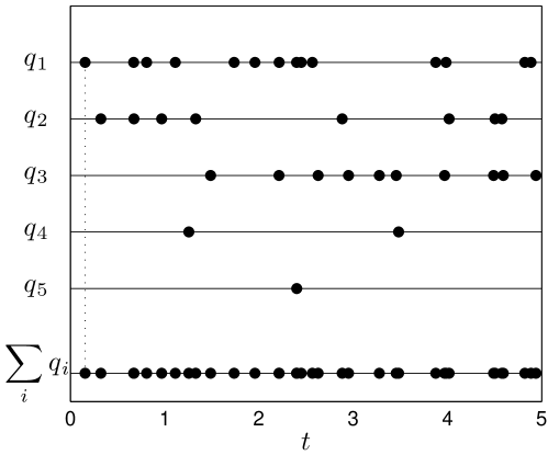
Let $(q_{1},q_{2},\ldots)$ be a countably infinite vector of feature probabilities. We begin by putting minimal restrictions on the $q_{i}$. We assume that they are strictly positive, decreasing real numbers. They need not necessarily sum to one, and they may be random. Indeed, we will eventually consider the case where the $q_{i}$ are the (random) atom weights of a beta process, and then we will have $\sum_{i}q_{i}\neq 1$ with probability one.

Let $\Pi_{i}$ be a standard Poisson process on the positive real line generated with rate $q_{i}$ (see, e.g., the top five lines in Figure 4). Then $\Pi:=\bigcup_{i}\Pi_{i}$ is a standard Poisson process on the positive real line with rate $\sum_{i}q_{i}$ (see, e.g., the lowermost line in Figure 4), where we henceforth assume $\sum_{i}q_{i}<\infty$ a.s.

Finally, as mentioned above, we define $K(t)$ to be the number of Poisson processes $\Pi_{i}$ with any points in $[0,t]$:

$$K(t):=\sum_{i}\mathbbm{1}\{|\Pi_{i}\cap[0,t]|>0\}.$$

And we define $K_{j}(t)$ to be the number of Poisson processes $\Pi_{i}$ with exactly $j$ points in $[0,t]$:

$$K_{j}(t):=\sum_{i}\mathbbm{1}\{|\Pi_{i}\cap[0,t]|=j\}.$$

These definitions are very similar to the definitions of $K_{N}$ and $K_{N,j}$ in Eqs. (8) and (7), respectively. The principal difference is that the $K_{N}$ are incremented only at integer $N$ whereas the $K(t)$ can have jumps at any $t\in\mathbb{R}_{+}$. The same observation holds for the $K_{N,j}$ and $K_{j}(t)$.

In addition to Poissonizing $K_{N}$ and $K_{N,j}$ to define $K(t)$ and $K_{j}(t)$, we will also find it convenient to assume that the $\{q_{i}\}$ themselves are derived from a Poisson process with rate measure $\nu$. We note that Poissonizing from a discrete index $N$ to a continuous time index $t$ is an approximation and separate from our assumption that the $\{q_{i}\}$ are generated from a Poisson process though both are fundamentally tied to the ease of working with Poisson processes.

We are now able to write out the mean feature counts in both the Poissonized and original cases. First, the Poissonized definitions of $\Phi$ and $K$ allow us to write

$$\Phi(t):=\mathbb{E}[K(t)]=\mathbb{E}[\mathbb{E}[K(t)|q]]=\mathbb{E}[\mathbb{E}[\sum_{i}\mathbbm{1}\{|\Pi_{i}\cap[0,t]|>0\}|q]].$$

With a similar approach for $\Phi_{j}(t)$, we find

$$\Phi(t)=\mathbb{E}[\sum_{i}(1-e^{-tq_{i}})],\quad\Phi_{j}(t)=\mathbb{E}[\sum_{i}\frac{(tq_{i})^{j}}{j!}e^{-tq_{i}}].$$

With the assumption that the $\{q_{i}\}$ are drawn from a Poisson process with measure measure $\nu$, we can apply Campbell’s theorem (Theorem 2) to both the original and Poissonized versions of the process to derive the final equality in each of the following lines

$$\Phi(t) =\mathbb{E}[\sum_{i}(1-e^{-tq_{i}})]=\int_{0}^{1}(1-e^{-tx})\;\nu(dx)$$ (23)

$$\Phi_{N} =\mathbb{E}[\sum_{i}(1-(1-q_{i})^{N})]=\int_{0}^{1}(1-(1-x)^{N})\;\nu(dx)$$ (24)

$$\Phi_{j}(t) =\mathbb{E}[\sum_{i}\frac{(tq_{i})^{j}}{j!}e^{-tq_{i}}]=\frac{t^{j}}{j!}\int_{0}^{1}x^{j}e^{-tx}\;\nu(dx)$$ (25)

$$\Phi_{N,j} =\binom{N}{j}\mathbb{E}[\sum_{i}q_{i}^{j}(1-q_{i})^{N-j}]=\binom{N}{j}\int_{0}^{1}x^{j}(1-x)^{N-j}\;\nu(dx).$$ (26)

Now we establish our first result, which gives a power law in $\Phi(t)$ and $\Phi_{j}(t)$ when the Poisson process rate measure $\nu$ has corresponding power law properties.

Proposition 3.

Asymptotic behavior of the integral of $\nu$ of the following form

$$\nu_{1}[0,x]:=\int_{0}^{x}u\;\nu(du)\sim\frac{\alpha}{1-\alpha}x^{1-\alpha}l(1/x),\quad x\rightarrow 0$$ (27)

where $l$ is a regularly varying function and $\alpha\in(0,1)$ implies

$$\Phi(t) \sim \Gamma(1-\alpha)t^{\alpha}l(t),\quad t\rightarrow\infty$$

$$\Phi_{j}(t) \sim \frac{\alpha\Gamma(j-\alpha)}{j!}t^{\alpha}l(t),\quad t\rightarrow\infty\quad(j>1).$$

Proof.

The key to this result is in the repeated use of Abelian or Tauberian theorems. Let $A$ be a map $A:F\rightarrow G$ from one function space to another: e.g., an integral or a Laplace transform. For $f\in F$, an Abelian theorem gives us the asymptotic behavior of $A(f)$ from the asymptotic behavior of $f$, and a Tauberian theorem gives us the asymptotic behavior of $f$ from that of $A(f)$.

First, integrating by parts yields

$$\nu_{1}[0,x]=-x\bar{\nu}(x)+\int_{0}^{x}\bar{\nu}(u)\;du,\quad\bar{\nu}(x):=\int_{x}^{\infty}\nu(u)\;du,$$

so the stated asymptotic behavior in $\nu_{1}$ yields $\bar{\nu}(x)\sim l(1/x)x^{-\alpha}(x\rightarrow 0)$ by a Tauberian theorem (Feller, 1966; Gnedin et al., 2007) where the map $A$ is an integral.

Second, another integration by parts yields

$$\Phi(t)=t\int_{0}^{\infty}e^{-tx}\bar{\nu}(x)\;dx.$$

The desired asymptotic behavior in $\Phi$ follows from the asymptotic behavior in $\bar{\nu}$ and an Abelian theorem (Feller, 1966; Gnedin et al., 2007) where the map $A$ is a Laplace transform. The result for $\Phi_{j}(t)$ follows from a similar argument when we note that repeated integration by parts of Eq. (25) also yields a Laplace transform. ∎

The importance of assuming that the $q_{i}$ are distributed according to a Poisson process is that this assumption allowed us to write $\Phi$ as an integral and thereby make use of classic Abelian and Tauberian theorems. The importance of Poissonizing the processes $K_{j}$ and $K_{N,j}$ is that we can write their means as in Eqs. (23) and (25), which are—up to integration by parts—in the form of Laplace transforms.

Proposition 3 is the most significant link in the chain of results needed to show asymptotic behavior of the feature counts $K_{N}$ and $K_{N,j}$ in that it relates power laws in the known feature probability rate measure $\nu$ to power laws in the mean behavior of the Poissonized version of these processes. It remains to show this mean behavior translates back to $K_{N}$ and $K_{N,j}$, first by relating the means of the original and Poissonized processes and then by relating the means to the almost sure behavior of the counts. The next two lemmas address the former concern. Together they establish that the mean feature counts $\Phi_{N}$ and $\Phi_{N,j}$ have the same asymptotic behavior as the corresponding Poissonized mean feature counts $\Phi(N)$ and $\Phi_{j}(N)$.

Lemma 4.

Let $\nu$ be $\sigma$-finite with $\int_{0}^{\infty}\nu(du)=\infty$ and $\int_{0}^{\infty}u\;\nu(du)<\infty$. Then the number of represented features has unbounded growth almost surely. The expected number of represented features has unbounded growth, and the expected number of features has sublinear growth. That is,

$$K(t)\uparrow\infty\textrm{ a.s}.,\quad\Phi(t)\uparrow\infty,\quad\Phi(t)\ll t.$$

Proof.

As in Gnedin et al. (2007), the first statement follows from the fact that $q$ is countably infinite and each $q_{i}$ is strictly positive. The second statement follows from monotone convergence. The final statement is a consequence of $\sum_{i}q_{i}<\infty$ a.s. ∎

Lemma 5.

Suppose the $\{q_{i}\}$ are generated according to a Poisson process with rate measure as in Lemma 4. Then, for $N\rightarrow\infty$,

$$|\Phi_{N}-\Phi(N)| <\frac{2}{N}\Phi_{2}(N)\rightarrow 0$$

$$|\Phi_{N,j}-\Phi_{j}(N)| <\frac{c_{j}}{N}\max\{\Phi_{j}(N),\Phi_{j+2}(N)\}\rightarrow 0.$$

for some constants $c_{j}$.

Proof.

The proof is the same as that of Lemma 1 of Gnedin et al. (2007). Establishing the inequalities results from algebraic manipulations. The convergence to zero is a consequence of Lemma 4. ∎

Finally, before considering the specific case of the three-parameter beta process, we wish to show that power laws in the means $\Phi_{N}$ and $\Phi_{N,j}$ extend to almost sure power laws in the number of represented features.

Proposition 6.

Suppose the $\{q_{i}\}$ are generated from a Poisson process with rate measure as in Lemma 4. For $N\rightarrow\infty$,

$$K_{N}\stackrel{{\scriptstyle a.s.}}{{\sim}}\Phi_{N},\quad\sum_{k<j}K_{N,k}\stackrel{{\scriptstyle a.s.}}{{\sim}}\sum_{k<j}\Phi_{N,k}.$$

Proof.

We wish to show that $K_{N}/\Phi_{N}\stackrel{{\scriptstyle a.s.}}{{\rightarrow}}1$ as $N\rightarrow\infty$. By Borel-Cantelli, it is enough to show that, for any $\epsilon>0$,

$$\sum_{N}\mathbb{P}\left(\left|\frac{K_{N}}{\Phi_{N}}-1\right|>\epsilon\right)<\infty.$$

To that end, note

$$\mathbb{P}\left(\left|K_{N}-\Phi_{N}\right|>\epsilon\Phi_{N}\right)\leq\mathbb{P}\left(\Phi_{N}>\epsilon\Phi_{N}+K_{N}\right)+\mathbb{P}\left(K_{N}>\epsilon\Phi_{N}+\Phi_{N}\right).$$

The note after Theorem 4 in Freedman (1973) gives that

$$\mathbb{P}\left(\Phi_{N}>\epsilon\Phi_{N}+K_{N}\right) \leq \exp\left(-\epsilon^{2}\Phi_{N}\right)$$

$$\mathbb{P}\left(K_{N}>\epsilon\Phi_{N}+\Phi_{N}\right) \leq \exp\left(-\frac{\epsilon^{2}}{1+\epsilon}\Phi_{N}\right).$$

So

$$\mathbb{P}\left(\left|\frac{K_{N}}{\Phi_{N}}-1\right|>\epsilon\right) \leq 2\exp\left(-2\epsilon^{2}\Phi_{N}\right)$$

$$\leq c\exp\left(-2\epsilon^{2}N\right)$$

for some constant $c$ and sufficiently large $N$ by Lemmas 4 and 5. The last expression is summable in $N$, and Borel-Cantelli holds.

The proof that $\quad\sum_{k<j}K_{N,k}\stackrel{{\scriptstyle a.s.}}{{\sim}}\sum_{k<j}\Phi_{N,j}$ follows the same argument. ∎

It remains to show that we obtain Type I and II power laws in our special case of the three-parameter beta process, which implies a particular rate measure $\nu$ in the Poisson process representation of the $\{q_{i}\}$. For the three-parameter beta process density in Eq. (15), we have

$$\nu_{1}[0,x] = \int_{\Psi\times(0,x]}u\;\nu_{BP}(d\psi,du)$$

$$= \gamma\cdot\frac{\Gamma(1+\theta)}{\Gamma(1-\alpha)\Gamma(\theta+\alpha)}\int_{0}^{x}u^{-\alpha}(1-u)^{\theta+\alpha-1}\;du$$

$$\sim \gamma\cdot\frac{\Gamma(1+\theta)}{\Gamma(1-\alpha)\Gamma(\theta+\alpha)}\int_{0}^{x}u^{-\alpha}\;du,\quad x\downarrow 0$$

$$= \gamma\cdot\frac{\Gamma(1+\theta)}{\Gamma(1-\alpha)\Gamma(\theta+\alpha)}\cdot\frac{1}{1-\alpha}x^{1-\alpha}.$$

The final line is exactly the form required by Eq. (27) in Proposition 3, with $l(y)$ equal to the constant function of value

$$C:=\frac{\gamma}{\alpha}\cdot\frac{\Gamma(1+\theta)}{\Gamma(1-\alpha)\Gamma(\theta+\alpha)}.$$ (28)

Then Proposition 3 implies that the following power laws hold for the mean of the Poissonized process:

$$\Phi(t) \stackrel{{\scriptstyle a.s.}}{{\sim}} \Gamma(1-\alpha)Ct^{\alpha},\quad t\rightarrow\infty$$

$$\Phi_{j}(t) \stackrel{{\scriptstyle a.s.}}{{\sim}} \frac{\alpha\Gamma(j-\alpha)}{j!}Ct^{\alpha},\quad t\rightarrow\infty\quad(j>1).$$

Lemma 5 further yields

$$\Phi_{N} \stackrel{{\scriptstyle a.s.}}{{\sim}} \Gamma(1-\alpha)CN^{\alpha},\quad N\rightarrow\infty$$

$$\Phi_{N,j} \stackrel{{\scriptstyle a.s.}}{{\sim}} \frac{\alpha\Gamma(j-\alpha)}{j!}CN^{\alpha},\quad N\rightarrow\infty\quad(j>1),$$

and finally Proposition 6 implies

$$K_{N} \stackrel{{\scriptstyle a.s.}}{{\sim}} \Gamma(1-\alpha)CN^{\alpha},\quad N\rightarrow\infty$$ (29)

$$K_{N,j} \stackrel{{\scriptstyle a.s.}}{{\sim}} \frac{d\Gamma(j-\alpha)}{j!}CN^{\alpha},\quad N\rightarrow\infty\quad(j>1).$$ (30)

These are exactly the desired Type I and II power laws (Eqs. (9) and (10)) for appropriate choices of the constants.

6.2 Exponential decay in the number of features

Next we consider a single data point and the number of features which are expressed for that data point in the featural model. We prove results for the general case where the $i$th feature has probability $q_{i}\geq 0$ such that $\sum_{i}q_{i}<\infty$. Let $Z_{i}$ be a Bernoulli random variable with success probability $q_{i}$ and such that all the $Z_{i}$ are independent. Then $\mathbb{E}[\sum_{i}Z_{i}]=\sum_{i}q_{i}=:Q$. In this case, a Chernoff bound (Chernoff, 1952; Hagerup and Rub, 1990) tells us that, for any $\delta>0$, we have

$$\mathbb{P}[\sum_{i}Z_{i}\geq(1+\delta)Q]\leq e^{\delta Q}(1+\delta)^{-(1+\delta)Q}.$$

When $M$ is large enough such that $M>Q$, we can choose $\delta$ such that $(1+\delta)Q=M$. Then this inequality becomes

$$\mathbb{P}[\sum_{i}Z_{i}\geq M]\leq e^{M-Q}Q^{M}M^{-M}\quad\textrm{for $M>Q$}.$$ (31)

We see from Eq. (31) that the number of features $\sum_{i}Z_{i}$ that are expressed for a data point exhibits super-exponential tail decay and therefore cannot have a power law probability distribution when the sum of feature probabilities $\sum_{i}q_{i}$ is finite. For comparison, let $Z\sim\textrm{Pois}(Q)$. Then (Franceschetti et al., 2007)

$$\mathbb{P}[Z\geq M]\leq e^{M-Q}Q^{M}M^{-M}\quad\textrm{for $M>Q$},$$

the same tail bound as in Eq. (31).

To apply the tail-behavior result of Eq. (31) to the beta process (with two or three parameters), we note that the total feature probability mass is finite by Eq. (16). Since the same set of feature probabilities is used in all subsequent Bernoulli process draws for the beta-Bernoulli process, the result holds.

7 Simulation

To illustrate the three types of power laws discussed above, we simulated beta process atom weights under three different choices of the discount parameter $\alpha$, namely $\alpha=0$ (the classic, two-parameter beta process), $\alpha=0.3$, and $\alpha=0.6$. In all three simulations, the remaining beta process parameters were kept constant at total mass parameter value $\gamma=3$ and concentration parameter value $\theta=1$.

The simulations were carried out using our extension of the Paisley et al. (2010) stick-breaking construction in Eq. (14). We generated 2,000 rounds of feature probabilities; that is, we generated 2,000 random variables $C_{i}$ and $\sum_{i=1}^{2,000}C_{i}$ feature probabilities. With these probabilities, we generated $N$ = 1,000 data points, i.e., 1,000 vectors of (2,000) independent Bernoulli random variables with these probabilities. With these simulated data, we were able to perform an empirical evaluation of our theoretical results.

Figure 5: Growth in the number of represented features $K_{N}$ (left) and the number of features represented by exactly one data point $K_{N,1}$ (right) as the total number of data points $N$ grows. The points in the scatterplot are derived by simulation; blue for $\alpha=0$, center black is $\alpha=0.3$, and upper black for $\alpha=0.6$. The red lines in the left plot show the theoretical mean $\Phi_{N}$ (Eq. (24)); in the right plot, they show the theoretical mean $\Phi_{N,1}$ (Eq. (26)). The green lines show the theoretical asymptotic behavior, Eq. (29) on the left (Type I power law) and Eq. (30) on the right (Type II power law).

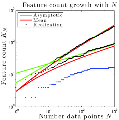
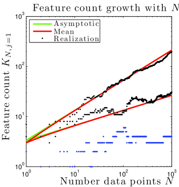
Figure 5 illustrates power laws in the number of represented features $K_{N}$ on the left (Type I power law) and the number of features represented by exactly one data point $K_{N,1}$ on the right (Type II power law). Both of these quantities are plotted as functions of the increasing number of data points $N$. The blue points show the simulated values for the classic, two-parameter beta process case with $\alpha=0$. The center set of black points in each case corresponds to $\alpha=0.3$, and the upper set of black points in each case corresponds to $\alpha=0.6$.

We also plot curves obtained from our theoretical results in order to compare them to the simulation. Recall that in our theoretical development, we noted that there are two steps to establishing the asymptotic behavior of $K_{N}$ and $K_{N,j}$ as $N$ increases. First, we compare the random quantities $K_{N}$ and $K_{N,j}$ to their respective means, $\Phi_{N}$ and $\Phi_{N,j}$. These means, as computed via numerical quadrature from Eq. (24) and directly from Eq. (26), are shown by red curves in the plots. Second, we compare the means to their own asymptotic behavior. This asymptotic behavior, which we ultimately proved was shared with the respective $K_{N}$ or $K_{N,j}$ in Eqs. (29) and (30), is shown by green curves in the plots.

We can see in both plots that the $\alpha=0$ behavior is distinctly different from the straight-line behavior of the $\alpha>0$ examples. In both cases, we can see that any growth in $\alpha$ is slower than can be described by straight-line growth. In particular, when $\alpha=0$, the expected number of features is

$$\phi_{N}=\mathbb{E}[K_{N}]=\mathbb{E}\left[\sum_{n=1}^{N}\textrm{Pois}\left(\gamma\frac{\theta}{n+\theta}\right)\right]\\ =\sum_{n=1}^{N}\gamma\frac{\theta}{n+\theta}\\ \sim\gamma\theta\log(N).$$ (32)

Similarly, when $\alpha=0$, the expected number of features represented by exactly one data point, $K_{N,1}$, is (by Eq. (26))

$$\Phi_{N,1} =\mathbb{E}[K_{N,1}]=\binom{N}{1}\int_{0}^{1}x^{1}(1-x)^{N-1}\cdot\theta x^{-1}(1-x)^{\theta-1}\;dx$$

$$=N\theta\cdot\frac{\Gamma(1)\Gamma(N-1+\theta)}{\Gamma(N+\theta)}=\theta\frac{N}{N-1+\theta}\sim\theta,$$

where the second line follows from using the normalization constant of the (proper) beta distribution. Interestingly, while $K_{N,1}$ grows as a power law when $\alpha>0$, its expectation is constant when $\alpha=0$. While many new features are instantiated as $N$ increases in the $\alpha=0$ case, it seems that they are quickly represented by more data points than just the first one.

Figure 6: Left: Change in the number of features with exactly $j$ representatives among $N$ data points for fixed $N$ as a function of $j$. The blue points, with connecting lines, are for $\alpha=0$; middle black are for $\alpha=0.3$, upper black for $\alpha=0.6$. The green lines show the theoretical asymptotic behavior in $j$ (Eqs. (10) and (11)) for the two $\alpha>0$ cases. Right: Change in the number of data points, indexed by $n$, with number of feature assignments $k_{n}$ greater than some positive, real-valued $M$ as $M$ increases. Neither the $\alpha=0$ case (blue) nor the $\alpha>0$ cases (black) exhibit Type III power laws.

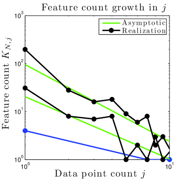
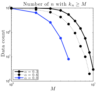
Type I and II power laws are somewhat easy to visualize since we have one point in our plots for each data point simulated. The behavior of $K_{N,j}$ as a function of $j$ for fixed $N$ and type III power laws (or lack thereof) are somewhat more difficult to visualize. In the case of $K_{N,j}$ as a function of $j$, we might expect that a large number of data points $N$ is necessary to see many groups of size $j$ for $j$ much greater than one. In the Type III case, we have seen that in fact power laws do not hold for any value of $\alpha$ in the beta process. Rather, the number of data points exhibiting more than $M$ features decreases more quickly in $M$ than a power law would predict; therefore, we cannot plot many values of $M$ before this number effectively goes to zero.

Nonetheless, Figure 6 compares our simulated data to the approximation of Eq. (10) with Eq. (11) (left) and Type III power laws (right). On the left, blue points as usual denote simulated data under $\alpha=0$; middle black points show $\alpha=0.3$, and upper black points show $\alpha=0.6$. Here, we use connecting lines between plotted points to clarify $\alpha$ values. The green lines for the $\alpha>0$ case illustrate the approximation of Eq. (11). Around $j=10$, we see that the number of feaures exhibited by $j$ data points, $K_{N,j}$, degenerates to mainly zero and one values. However, for smaller values of $j$ we can still distinguish the power law trend.

On the right-hand side of Figure 6, we display the number of data points exhibiting more than $M$ features for various values of $M$ across the three values of $\alpha$. Unlike the previous plots in Figure 5 and Figure 6, there is no power-law behavior for the cases $\alpha>0$, as predicted in Section 6.2. We also note that here the $\alpha=0.3$ curve does not lie between the $\alpha=0$ and $\alpha=0.6$ curves. Such an occurrence is not unusual in this case since, as we saw in Eq. (31), the rate of decrease is modulated by the total mass of the feature probabilities drawn from the beta process, which is random and not necessarily smaller when $\alpha$ is smaller.

Figure 7: Feature probabilities from the beta process plotted in decreasing size order. Blue points represent probabilities from the $\alpha=0$ case; center black points show $\alpha=0.3$, and upper black points show $\alpha=0.6$. The green lines show theoretical asymptotic behavior of the ranked probabilities (Eq. (33)).

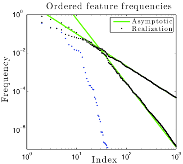
Finally, since our experiment involves generating the underlying feature probabilities from the beta process as well as the actual feature assignments from repeated draws from the Bernoulli process, we may examine the feature probabilities themselves; see Figure 7. As usual, the blue points represent the classic, two-parameter ($\alpha=0$) beta process. Black points represent $\alpha=0.3$ (center) and $\alpha=0.6$ (upper). Perhaps due to the fact that there is only the beta process noise to contend with in this aspect of the simulation (and not the combined randomness due to the beta process and Bernoulli process), we see the most striking demonstration of both power law behavior in the $\alpha>0$ cases and faster decay in the $\alpha=0$ case in this figure. The two $\alpha>0$ cases clearly adhere to a power law that may be predicted from our results above and the Gnedin et al. (2007) results with $C$ as in Eq. (28):

$$\#\{i:q_{i}\geq x\}\stackrel{{\scriptstyle a.s.}}{{\sim}}Cx^{-\alpha}\quad x\downarrow 0.$$ (33)

Note that ranking the probabilities merely inverts the plot that would be created with $x$ on the horizontal axis and $\{i:q_{i}\geq x\}$ on the vertical axis. The simulation demonstrates little noise about these power laws beyond the 100th ranked probability. The decay for $\alpha=0$ is markedly faster than the other cases.

8 Experimental results

We have seen that the Poisson process formulation allows for an easy extension of the beta process to a three-parameter model. In this section we study this model empirically in the setting of the modeling of handwritten digits. Paisley et al. (2010) present results for this problem using a two-parameter beta process coupled with a discrete factor analysis model; we repeat those experiments with the three-parameter beta process. The data consists of 3,000 examples of handwritten digits, in particular 1,000 handwriting samples of each of the digits 3, 5, and 8 from the MNIST Handwritten Digits database (LeCun and Cortes, 1998; Roweis, 2007). Each handwritten digit is represented by a matrix of 28$\times$28 pixels; we project these matrices into 50 dimensions using principal components analysis. Thus, our data takes the form $X\in\mathbb{R}^{50\times 3000}$, and we may apply the beta process factor model from Eq. (2) with $P=50$ and $N$ = 3,000 to discover latent structure in this data.

The generative model for $X$ that we use is as follows (see Paisley et al., 2010):

$$X =(W\circ Z)\Phi+E$$

$$Z \sim\textrm{BP-BeP}(N,\gamma,\theta,\alpha)$$

$$\Phi_{k,p} \stackrel{{\scriptstyle iid}}{{\sim}}N(0,\rho_{p})$$

$$W_{n,k} \stackrel{{\scriptstyle iid}}{{\sim}}N(0,\zeta)$$

$$E_{n,p} \stackrel{{\scriptstyle iid}}{{\sim}}N(0,\eta),$$ (34)

with hyperparameters $\theta,\alpha,\gamma,B_{0},\{\rho_{p}\}_{p=1}^{P},\zeta,\eta$. Recall from Eq. (2) that $X\in\mathbb{R}^{N\times P}$ is the data, $\Phi\in\mathbb{R}^{K\times P}$ is a matrix of factors, and $E\in\mathbb{R}^{N\times P}$ is an error matrix. Here, we introduce the weight matrix $W\in\mathbb{R}^{N\times K}$, which modulates the binary factor loadings $Z\in\mathbb{R}^{N\times K}$. In Eq. (34), $\circ$ denotes elementwise multiplication, and the indices have ranges $n\in\{1,\ldots,N\},k\in\{1,\ldots,K\},p\in\{1,\ldots,P\}$. Since we draw $Z$ from a beta-Bernoulli process, the dimension $K$ is theoretically infinite in the generative model notation of Eq. (34). However, we have seen that the number of columns of $Z$ with nonzero entries is finite a.s. We use $K$ to denote this number.

We initialized both the two-parameter and the three-parameter models with the same number of latent features, $K=200$, and the same values for all shared parameters (i.e., every variable except the new discount parameter $\alpha$). We ran the experiment for 2,000 MCMC iterations, noting that the MCMC runs in both models seem to have reached equilibrium by 500 iterations (see Figures 8 and 9).

Figure 8: The number of latent features $K$ as a function of the MCMC iteration. Results for the original, two-parameter model are represented on the left, and results for the new, three-parameter model are illustrated on the right.

Figure 9: The random values drawn for the hyperparameters as a function of the MCMC iteration. Draws for the concentration parameter $\theta$ under the two-parameter model are shown on the left, and draws for $\theta$ under the three-parameter model are shown in the middle. On the right are draws of the new discount parameter $\alpha$ under the three-parameter model.

Figure 10: Autocorrelation of the number of factors $K$, concentration parameter $\theta$, and discount parameter $\alpha$ for the MCMC samples after burn-in (where burn-in is taken to end at 500 iterations) under the two-parameter model (left) and three-parameter model (right).

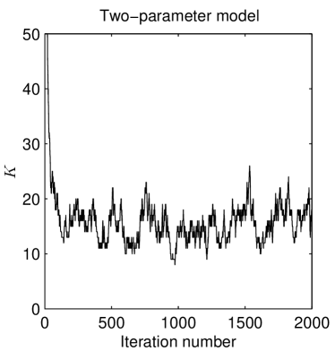
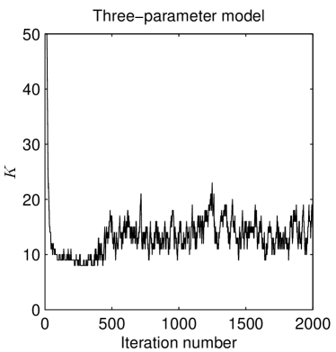
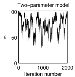
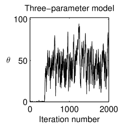
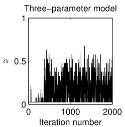
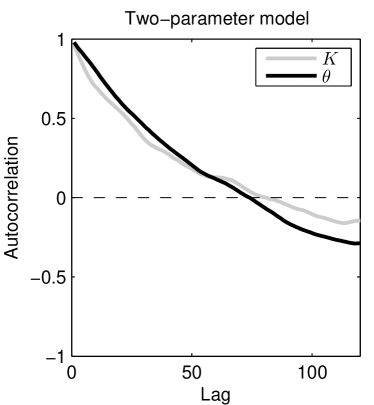
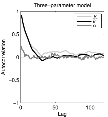
Figures 8 and 9 show the sampled values of various parameters as a function of MCMC iteration. In particular, we see how the number of features $K$ (Figure 8), the concentration parameter $\theta$, and the discount parameter $\alpha$ (Figure 9) change over time. All three graphs illustrate that the three-parameter model takes a longer time to reach equilibrium than the two-parameter model (approximately 500 iterations vs. approximatively 100 iterations). However, once at equilibrium, the sampling time series associated with the three-parameter iterations exhibit lower autocorrelation than the samples associated with the two-parameter iterations (Figure 10). In the implementation of both the original two-parameter model and the three-parameter model, the range for $\theta$ is considered to be bounded above by approximately 100 for computational reasons (in accordance with the original methodology of Paisley et al. (2010)). As shown in Figure 9, this bound affects sampling in the two-parameter experiment whereas, after burn-in, the effect is not noticeable in the three-parameter experiment. While the discount parameter $\alpha$ also comes close to the lower boundary of its discretization (Figure 9)—which cannot be exactly zero due to computational concerns—the samples nonetheless seem to explore the space well.

We can see from Figure 10 that the estimated value of the concentraton parameter $\theta$ is much lower when the discount parameter $\alpha$ is also estimated. This behavior may be seen to result from the fact that the power law growth of the expected number of represented features $\Phi_{N}$ in the $\alpha>0$ case yields a generally higher expected number of features than in the $\alpha=0$ case for a fixed concentration parameter $\theta$. Further, we see from Eq. (32) that the expected number of features when $\alpha=0$ is linear in $\theta$. Therefore, if we instead fix the number of features, the $\alpha=0$ model can compensate by increasing $\theta$ over the $\alpha>0$ model. Indeed, we see in Figure 8 that the number of features discovered by both models is roughly equal; in order to achieve this number of features, the $\alpha=0$ model seems to be compensating by overestimating the concentration parameter $\theta$.

Two-parameter model

Three-parameter model

Figure 11: Upper: The top nine features by sampled representation across the data set on the final MCMC iteration for the original, two-parameter model. Lower: The top nine features determined in the same way for the new, three-parameter model.

To get a sense of the actual output of the model, we can look at some of the learned features. In particular, we collected the set of features from the last MCMC iteration in each model. The $k$th feature is expressed or not for the $n$th data point according to whether $Z_{nk}$ is one or zero. Therefore, we can find the most-expressed features across the data set using the set of features on this iteration as well as the sampled $Z$ matrix on this iteration. We plot the nine most-expressed features under each model in Figure 11. In both models, we can see how the features have captured distinguishing features of the 3, 5, and 8 digits.

Finally, we note that the three-parameter version of the algorithm is competitive with the two-parameter version in running time once equilibrium is reached. After the burn-in regime of 500 iterations, the average running time per iteration under the three-parameter model is 14.5 seconds, compared with 11.7 seconds average running time per iteration under the two-parameter model.

9 Conclusions

We have shown that the stick-breaking representation of the beta process due to Paisley et al. (2010) can be obtained directly from the representation of the beta process as a completely random measure. With this result in hand the set of connections between the beta process, stick-breaking, and the Indian buffet process are essentially as complete as those linking the Dirichlet process, stick-breaking, and the Chinese restaurant process.

We have also shown that this approach motivates a three-parameter generalization of the stick-breaking representation of Paisley et al. (2010), which is the analog of the Pitman-Yor generalization of the stick-breaking representation for the Dirichlet process. We have shown that Type I and Type II power laws follow from this three-parameter model. We have also shown that Type III power laws cannot be obtained within this framework. It is an open problem to discover useful classes of stochastic processes that provide such power laws.

10 Acknowledgments

We wish to thank Alexander Gnedin for useful discussions and Lancelot James for helpful suggestions. We also thank John Paisley for useful discussions and for kindly providing access to his code, which we used in our experimental work. Tamara Broderick was funded by a National Science Foundation Graduate Research Fellowship. Michael Jordan was supported in part by IARPA-BAA-09-10, “Knowledge Discovery and Dissemination.” Jim Pitman was supported in part by the National Science Foundation Award 0806118 “Combinatorial Stochastic Processes.”

Appendix A A Markov chain Monte Carlo algorithm

Posterior inference under the three-parameter model can be performed with a Markov chain Monte Carlo (MCMC) algorithm. Many conditionals have simple forms that allow Gibbs sampling although others require further approximation. Most of our sampling steps are as in Paisley et al. (2010) with the notable exceptions of a new sampling step for the discount parameter $\alpha$ and integration of the discount parameter $\alpha$ into the existing framework. We describe the full algorithm here.

A.1 Notation and auxiliary variables

Call the index $i$ in Eq. (14) the round. Then introduce the round-indicator variables $r_{k}$ such that $r_{k}=i$ exactly when the $k$th atom, where $k$ indexes the sequence $(\psi_{1,1},\ldots,\psi_{1,C_{1}},\psi_{2,1},\ldots,\psi_{2,C_{2}},\ldots)$, occurs in round $i$. We may write

$$r_{k}:=1+\sum_{i=1}^{\infty}\mathbbm{1}\left\{\sum_{j=1}^{i}C_{j}<k\right\}.$$

To recover the round lengths $C$ from $r=(r_{1},r_{2},\ldots)$, note that

$$C_{i}=\sum_{k=1}^{\infty}\mathbbm{1}(r_{k}=i).$$ (35)

With the definition of the round indicators $r$ in hand, we can rewrite the beta process $B$ as

$$B=\sum_{k=1}^{\infty}V_{k,r_{k}}\prod_{j=1}^{r_{k}}(1-V_{k,j})\delta_{\psi_{k}},$$

where $V_{k,j}\stackrel{{\scriptstyle iid}}{{\sim}}\textrm{Beta}(1-\alpha,\theta+i\alpha)$ and $\psi_{k}\stackrel{{\scriptstyle iid}}{{\sim}}\gamma^{-1}B_{0}$ as usual although the indexing is not the same as in Eq. (14). It follows that the expression of the $k$th feature for the $n$th data point is given by

$$Z_{n,k}\sim\textrm{Bern}\left(\pi_{k}\right),\quad\pi_{k}:=V_{k,r_{k}}\prod_{j=1}^{r_{k}-1}(1-V_{k,j}).$$

We also introduce notation for the number of data points in which the $k$th feature is, respectively, expressed and not expressed:

$$m_{1,k}:=\sum_{n=1}^{N}\mathbbm{1}(Z_{n,k}=1),\quad m_{0,k}:=\sum_{n=1}^{N}\mathbbm{1}(Z_{n,k}=0)$$

Finally, let $K$ be the number of represented features; i.e., $K:=\#\{k:m_{1,k}>0\}$. Without loss of generality, we assume the represented features are the first $K$ features in the index $k$. The new quantities $\{r_{k}\}$, $\{m_{1,k}\}$, $\{m_{0,k}\}$, and $K$ will be used in describing the sampler steps below.

A.2 Latent indicators

First, we describe the sampling of the round indicators $\{r_{k}\}$ and the latent feature indicators $\{Z_{n,k}\}$. In these and other steps in the MCMC algorithm, we integrate out the stick-breaking proportions $\{V_{i}\}$.

A.2.1 Round indicator variables

We wish to sample the round indicator $r_{k}$ for each feature $k$ with $1\leq k\leq K$. We can write the conditional for $r_{k}$ as

$$p(r_{k}=i|\{r_{l}\}_{l=1}^{k-1},\{Z_{n,k}\}_{n=1}^{N},\theta,\alpha,\gamma)$$ (36)

$$\propto p(\{Z_{n,k}\}_{n=1}^{N}|r_{k}=i,\theta,\alpha)p(r_{k}=i|\{r_{l}\}_{l=1}^{k-1}).$$

It remains to calculate the two factors in the product.

For the first factor in Eq. (36), we write out the integration over stick-breaking proportions and approximate with a Monte Carlo integral:

$$p(\{Z_{n,k}\}_{n=1}^{N}|r_{k}=i,\theta,\alpha) = \int_{[0,1]^{i}}\pi_{k}^{m_{1,k}}(1-\pi_{k})^{m_{0,k}}\;dV$$ (37)

$$\approx \frac{1}{S}\sum_{s=1}^{S}(\pi_{k}^{(s)})^{m_{1,k}}(1-\pi_{k}^{(s)})^{m_{0,k}}.$$

Here, $\pi^{(s)}_{k}:=V^{(s)}_{k,r_{k}}\prod_{j=1}^{r_{k}-1}(1-V^{(s)}_{k,j})$, and $V_{k,j}^{(s)}\stackrel{{\scriptstyle indep}}{{\sim}}\textrm{Beta}(1-\alpha,\theta+j\alpha)$. Also, $S$ is the number of samples in the sum approximation. Note that the computational trick employed in Paisley et al. (2010) for sampling the $\{V_{i}\}$ relies on the first parameter of the beta distribution being equal to one; therefore, the sampling described above, without further tricks, is exactly the sampling that must be used in this more general parameterization.

For the second factor in Eq. (36), there is no dependence on the $\alpha$ parameter, so the draws are the same as in Paisley et al. (2010). For $R_{k}:=\sum_{j=1}^{k}\mathbbm{1}(r_{j}=r_{k})$, we have

$$p(r_{k}=r|\gamma,\{r_{l}\}_{l=1}^{k-1})$$

$$= \left\{\begin{array}[]{ll}0&r<r_{k-1}\\ \frac{1-\sum_{i=1}^{R_{k-1}}\textrm{Pois}(i|\gamma)}{1-\sum_{i=1}^{R_{k-1}-1}\textrm{Pois}(i|\gamma)}&r=r_{k-1}\\ \left(1-\frac{1-\sum_{i=1}^{R_{k-1}}\textrm{Pois}(i|\gamma)}{1-\sum_{i=1}^{R_{k-1}-1}\textrm{Pois}(i|\gamma)}\right)\left(1-\textrm{Pois}(0|\gamma)\right)\textrm{Pois}(0|\gamma)^{h-1}&r=r_{k-1}+h\end{array}\right.$$

for each $h\geq 1$. Note that these draws make the approximation that the first $K$ features correspond to the first $K$ tuples $(i,j)$ in the double sum of Eq. (14); these orderings do not in general agree.

To complete the calculation of the posterior for $r_{k}$, we need to sum over all values of $i$ to normalize $p(r_{k}=i|\{r_{l}\}_{l=1}^{k-1},\{Z_{n,k}\}_{n=1}^{N},\theta,\alpha,\gamma)$. Since this is not computationally feasible, an alternative method is to calculate Eq. (36) for increasing values of $i$ until the result falls below a pre-determined threshold.

A.2.2 Factor indicators

In finding the posterior for the $k$th feature indicator in the $n$th latent factor, $Z_{n,k}$, we can integrate out both $\{V_{i}\}$ and the weight variables $\{W_{n,k}\}$. The conditional for $Z_{n,k}$ is

$$p(Z_{n,k}|X_{n,\cdot},\Phi,Z_{n,-k},r,\theta,\alpha,\eta,\zeta)$$ (39)

$$= p(X_{n,\cdot}|Z_{n,\cdot},\Phi,\eta,\zeta)p(Z_{n,k}|r,\theta,\alpha,Z_{n,-k}).$$

First, we consider the likelihood. For this factor, we integrate out $W$ explicitly:

$$p(X_{n,\cdot}|Z_{n,\cdot},\Phi,\eta,\zeta)$$

$$= \int_{W}p(X_{n,\cdot}|Z_{n,\cdot},\Phi,W,\eta)p(W|\zeta)$$

$$= \int_{W_{n,I}}N(X_{n,\cdot}|W_{n,I}\Phi_{I,\cdot},\eta I_{P})N(W_{n,I}|0_{|I|},\zeta I_{|I|})dW_{n,I}$$

where $$I=\{i:Z_{n,i}=1\}$$

$$= N\left(X_{n,\cdot}|0_{P},\left[\eta^{-1}I_{P}-\eta^{-2}\Phi_{I,\cdot}\left(\eta^{-1}\Phi_{I,\cdot}^{\top}\Phi_{I,\cdot}+\zeta^{-1}I_{|I|}\right)^{-1}\Phi_{I,\cdot}^{\top}\right]^{-1}\right)$$

$$= N\left(X_{n,\cdot}|0_{P},\eta I_{P}+\zeta\Phi_{I,\cdot}\Phi_{I,\cdot}^{\top}\right),$$

where the final step follows from the Sherman-Morrison-Woodbury lemma.

For the second factor in Eq. (39), we can write

$$p(Z_{n,k}|r,\theta,\alpha,Z_{n,-k}) = \frac{p(Z_{n}|r,\theta,\alpha)}{p(Z_{n,-k}|r,\theta,\alpha)},$$

and the numerator and denominator can both be estimated as integrals over $V$ using the same Monte Carlo integration trick as in Eq. (37).

A.3 Hyperparameters

Next, we describe sampling for the three parameters of the beta process. The mass and concentration parameters are shared by the two-parameter process; the discount parameter is unique to the three-parameter beta process.

A.3.1 Mass parameter

With the round indicators $\{r_{k}\}$ in hand as from Appendix A.2.1 above, we can recover the round lengths $\{C_{i}\}$ with Eq. (35). Assuming an improper gamma prior on $\gamma$—with both shape and inverse scale parameters equal to zero—and recalling the iid Poisson generation of the $\{C_{i}\}$, the posterior for $\gamma$ is

$$p(\gamma|r,Z,\theta,\alpha)=\textrm{Ga}(\gamma|\sum_{i=1}^{r_{K}}C_{i},r_{K}).$$

Note that it is necessary to sample $\gamma$ since it occurs in, e.g., the conditional for the round indicator variables (Appendix A.2.1).

A.3.2 Concentration parameter

The conditional for $\theta$ is

$$p(\theta|Z,r,\alpha)\propto p(\theta)\prod_{k=1}^{K}p(Z|r,\theta,\alpha).$$

Again, we calculate the likelihood factors $p(Z|r,\theta,\alpha)$ with a Monte Carlo approximation as in Eq. (37). In order to find the conditional over $\theta$ from the likelihood and prior, we further approximate the space of $\theta>0$ by a discretization around the previous value of $\theta$ in the Monte Carlo sampler: $\{\theta_{prev}+t\Delta\theta\}_{t=S}^{t=T}$, where $S$ and $T$ are chosen so that all potential new $\theta$ values are nonnegative and so that the tails of the distribution fall below a pre-determined threshold. To complete the description, we choose the improper prior $p(\theta)\propto 1$.

A.3.3 Discount parameter

We sample the discount parameter $\alpha$ in a similar manner to $\theta$. The conditional for $\alpha$ is

$$p(\alpha|Z,r,\theta)\propto p(\alpha)\prod_{k=1}^{K}p(Z|r,\theta,\alpha).$$

As usual, we calculate the likelihood factors $p(Z|r,\theta,\alpha)$ with a Monte Carlo approximation as in Eq. (37). While we discretize the sampling of $\alpha$ as we did for $\theta$, note that sampling $\alpha$ is more straightforward since $\alpha$ must lie in $[0,1]$. Therefore, the choice of $\Delta\alpha$ completely characterizes the discretization of the interval. In particular, to avoid endpoint behavior, we consider new values of $\alpha$ among $\{\Delta\alpha/2+t\Delta\alpha\}_{t=0}^{(\Delta\alpha)^{-1}-1}$. Moreover, the choice of $p(\alpha)\propto 1$ is, in this case, a proper prior for $\alpha$.

A.4 Factor analysis components

In order to use the beta process as a prior in the factor analysis model described in Eq. (2), we must also describe samplers for the feature matrix $\Phi$ and weight matrix $W$.

A.4.1 Feature matrix

The conditional for the feature matrix $\Phi$ is

$$p(\Phi_{\cdot,p}|X,W,Z,\eta,\rho_{p}) \propto p(X_{\cdot,p}|\Phi_{\cdot,p},W,Z,\eta I_{N})p(\Phi_{\cdot,p}|\rho_{p})$$

$$= N(X_{\cdot,p}|(W\circ Z)\Phi_{\cdot,p},\eta I_{N})N(\Phi_{\cdot,p}|0_{K},\rho_{p}I_{K})$$

$$\propto N\left(\Phi_{\cdot,p}|\mu,\Sigma\right),$$

where, in the final line, the variance is defined as follows:

$$\Sigma:=\left(\eta^{-1}(W\circ Z)^{\top}(W\circ Z)+\rho_{p}^{-1}I_{K}\right)^{-1},$$

and similarly for the mean:

$$\mu:=\Sigma\eta^{-1}(W\circ Z)^{\top}X_{\cdot,p}.$$

A.4.2 Weight matrix

Let $I=\{i:Z_{n,i}=1\}$. Then the conditional for the weight matrix $W$ is

$$p(W_{n,I}|X,Z,\Phi,\eta) \propto p(X_{n,\cdot}|\Phi_{I,\cdot},W_{n,I},\eta)p(W_{n,I}|\zeta)$$

$$= N(X_{n,\cdot}|W_{n,I}\Phi_{I,\cdot},\eta I_{p})N(W_{n,I}|0_{|I|},\zeta I_{|I|})$$

$$\propto N(W_{n,I}|\tilde{\mu},\tilde{\Sigma}),$$

where, in the final line, the variance is defined as $\tilde{\Sigma}:=\left(\eta^{-1}\Phi_{I,\cdot}\Phi_{I,\cdot}^{\top}+\zeta^{-1}I_{|I|}\right)^{-1}$, and the mean is defined as $\tilde{\mu}:=\tilde{\Sigma}\eta^{-1}X_{n,\cdot}\Phi_{I,\cdot}^{\top}$.

References

- Blei and Jordan [2006] D. M. Blei and M. I. Jordan. Variational inference for Dirichlet process mixtures. Bayesian Analysis, 1(1):121–144, 2006.
- Chernoff [1952] H. Chernoff. A measure of asymptotic efficiency for tests of a hypothesis based on the sum of observations. The Annals of Mathematical Statistics, pages 493–507, 1952.
- Feller [1966] W. Feller. An Introduction to Probability Theory and Its Applications, Vol. II. John Wiley, New York, 1966.
- Ferguson [1973] T. S. Ferguson. A Bayesian analysis of some nonparametric problems. The Annals of Statistics, 1(2):209–230, 1973. ISSN 0090-5364.
- Franceschetti et al. [2007] M. Franceschetti, O. Dousse, D. N. C. Tse, and P. Thiran. Closing the gap in the capacity of wireless networks via percolation theory. Information Theory, IEEE Transactions on, 53(3):1009–1018, 2007.
- Freedman [1973] D. Freedman. Another note on the Borel–Cantelli lemma and the strong law, with the Poisson approximation as a by-product. The Annals of Probability, 1(6):910–925, 1973.
- Gnedin et al. [2007] A. Gnedin, B. Hansen, and J. Pitman. Notes on the occupancy problem with infinitely many boxes: General asymptotics and power laws. Probability Surveys, 4:146–171, 2007.
- Goldwater et al. [2006] S. Goldwater, T. Griffiths, and M. Johnson. Interpolating between types and tokens by estimating power-law generators. In Advances in Neural Information Processing Systems, 18, Cambridge, MA, 2006. MIT Press.
- Griffiths and Ghahramani [2006] T. Griffiths and Z. Ghahramani. Infinite latent feature models and the Indian buffet process. In Advances in Neural Information Processing Systems, 18, volume 18, Cambridge, MA, 2006. MIT Press.
- Hagerup and Rub [1990] T. Hagerup and C. Rub. A guided tour of Chernoff bounds. Information Processing Letters, 33(6):305–308, 1990.
- Heaps [1978] H. S. Heaps. Information Retrieval: Computational and Theoretical Aspects. Academic Press, Orlando, FL, 1978. ISBN 0123357500.
- Hjort [1990] N. L. Hjort. Nonparametric Bayes estimators based on beta processes in models for life history data. The Annals of Statistics, 18(3):1259–1294, 1990. ISSN 0090-5364.
- Ishwaran and James [2001] H. Ishwaran and L. F. James. Gibbs sampling methods for stick-breaking priors. Journal of the American Statistical Association, 96(453):161–173, 2001. ISSN 0162-1459.
- Kalli et al. [2009] M. Kalli, J. E. Griffin, and S. G. Walker. Slice sampling mixture models. Statistics and Computing, 21:93–105, 2009.
- Kim and Lee [2001] Y. Kim and J. Lee. On posterior consistency of survival models. Annals of Statistics, pages 666–686, 2001.
- Kingman [1967] J. F. C. Kingman. Completely random measures. Pacific Journal of Mathematics, 21(1):59–78, 1967.
- Kingman [1993] J. F. C. Kingman. Poisson Processes. Oxford University Press, 1993. ISBN 0198536933.
- LeCun and Cortes [1998] Y. LeCun and C. Cortes. The MNIST database of handwritten digits, 1998.
- MacEachern [1999] S. N. MacEachern. Dependent nonparametric processes. In ASA Proceedings of the Section on Bayesian Statistical Science, pages 50–55, 1999.
- McCloskey [1965] J. W. McCloskey. A model for the distribution of individuals by species in an environment. PhD thesis, Michigan State University, 1965.
- Mitzenmacher [2004] M. Mitzenmacher. A brief history of generative models for power law and lognormal distributions. Internet Mathematics, 1(2):226–251, 2004. ISSN 1542-7951.
- Paisley et al. [2010] J. Paisley, A. Zaas, C. W. Woods, G. S. Ginsburg, and L. Carin. A stick-breaking construction of the beta process. In International Conference on Machine Learning, Haifa, Israel, 2010.
- Paisley et al. [2011] J. Paisley, D. Blei, and M. I. Jordan. The stick-breaking construction of the beta process as a poisson process. Pre-print arXiv:1109.0343v1 [math.ST], 2011.
- Patil and Taillie [1977] G. P. Patil and C. Taillie. Diversity as a concept and its implications for random communities. In Proceedings of the 41st Session of the International Statistical Institute, pages 497–515, New Delhi, 1977.
- Pitman [2006] J. Pitman. Combinatorial stochastic processes, volume 1875 of Lecture Notes in Mathematics. Springer-Verlag, Berlin, 2006. URL http://bibserver.berkeley.edu/csp/april05/bookcsp.pdf.
- Pitman and Yor [1997] J. Pitman and M. Yor. The two-parameter Poisson-Dirichlet distribution derived from a stable subordinator. The Annals of Probability, 25(2):855–900, 1997. ISSN 0091-1798.
- Roweis [2007] S. Roweis. MNIST handwritten digits, 2007. URL http://www.cs.nyu.edu/~roweis/data.html.
- Sethuraman [1994] J. Sethuraman. A constructive definition of Dirichlet priors. Statistica Sinica, 4(2):639–650, 1994.
- Teh and Görür [2009] Y. W. Teh and D. Görür. Indian buffet processes with power-law behavior. In Advances in Neural Information Processing Systems, Cambridge, MA, 2009. MIT Press.
- Teh et al. [2007] Y. W. Teh, D. Görür, and Z. Ghahramani. Stick-breaking construction for the Indian buffet process. In Proceedings of the International Conference on Artificial Intelligence and Statistics, 11, San Juan, Puerto Rico, 2007.
- Thibaux and Jordan [2007] R. Thibaux and M. I. Jordan. Hierarchical beta processes and the Indian buffet process. In International Conference on Artificial Intelligence and Statistics, San Juan, Puerto Rico, 2007.
- Tricomi and Erdélyi [1951] F. G. Tricomi and A. Erdélyi. The asymptotic expansion of a ratio of gamma functions. Pacific Journal of Mathematics, 1(1):133–142, 1951.
- Walker [2007] S. G. Walker. Sampling the Dirichlet mixture model with slices. Communications in Statistics—Simulation and Computation, 36(1):45–54, 2007.
- Wolpert and Ickstadt [2004] R. L. Wolpert and K. Ickstadt. Reflecting uncertainty in inverse problems: A Bayesian solution using Lévy processes. Inverse Problems, 20:1759–1771, 2004.
- Zipf [1949] G. K. Zipf. Human Behaviour and the Principle of Least-Effort. Addison-Wesley, 1949.