Activity-Based Search
for Black-Box Contraint-Programming Solvers

Abstract

Robust search procedures are a central component in the design of black-box constraint-programming solvers. This paper proposes activity-based search, the idea of using the activity of variables during propagation to guide the search. Activity-based search was compared experimentally to impact-based search and the wdeg heuristics. Experimental results on a variety of benchmarks show that activity-based search is more robust than other heuristics and may produce significant improvements in performance.

1 Introduction

Historically, the constraint-programming (CP) community has focused on developing open, extensible optimization tools, where the modeling and the search procedure can be specialized to the problem at hand. This focus stems partially from the roots of CP in programming languages and partly from the rich modeling language typically found in CP systems. While this flexibility is appealing for experts in the field, it places significant burden on practitioners, reducing its acceptance across the wide spectrum of potential users. In recent years however, the constraint-programming community devoted increasing attention to the development of black-box constraint solvers. This new focus was motivated by the success of Mixed-Integer Programming (MIP) and SAT solvers on a variety of problem classes. MIP and SAT solvers are typically black-box systems with automatic model reformulations and general-purpose search procedures. As such, they allow practitioners to focus on modeling aspects and may reduce the time to solution significantly.

This research is concerned with one important aspect of black-box solvers: the implementation of a robust search procedure. In recent years, various proposals have addressed this issue. Impact-based search (Ibs) [10] is motivated by concepts found in MIP solvers such as strong branching and pseudo costs. Subsequent work about solution counting can be seen as an alternative to impacts [8] that exploits the structure of CP constraints. The weighted-degree heuristic (wdeg) [1] is a direct adaptation of the SAT heuristic Vsids[5] to CSPs that relies on information collected from failures to define the variable ordering.

This paper proposes Activity-Based Search (Abs), a search heuristic that recognizes the central role of constraint propagation in constraint-programming systems. Its key idea is to associate with each variable a counter which measures the activity of a variable during propagation. This measure is updated systematically during search and initialized by a probing process. Abs has a number of advantages compared to earlier proposals. First, it does not deal explicitly with variable domains which complicates the implementation and runtime requirements of Ibs. Second, it does not instrument constraints which is a significant burden in solution-counting heuristics. Third, it naturally deals with global constraints, which is not the case of wdeg since all variables in a failed constraint receive the same weight contribution although only a subset of them is relevant to the conflict. Abs was compared experimentally to Ibs and wdeg on a variety of benchmarks. The results show that Abs is the most robust heuristic and can produce significant improvements in performance over Ibs and wdeg, especially when the problem complexity increases.

The rest of the paper is organized as follows. Sections 2 and 3 review the Ibs and wdeg heuristics. Section 4 presents Abs. Section 5 presents the experimental results and Section 6 concludes the paper.

2 Impact-Based Search

Impact-based search was motivated by the concept of pseudo-cost in MIP solvers. The idea is to associate with a branching decision $x=v$ a measure of how effectively it shrinks the search space. This measure is called the impact of the branching decision.

Formalization

Let $P=\langle X,D,C\rangle$ be a CSP defined over variables $X$, domains $D$, and constraints $C$. Let $D(x_{i})$ denote the domain of variable $x_{i}\in X$ and $|D(x_{i})|$ denote the size of this domain. A trivial upper-bound on the size of the search space of ${\cal S}(P)$ is given by the product of the domain sizes:

$${\cal S}(P)=\prod_{x\in X}|D(x)|$$

At node $k$, the search procedure receives a CSP $P_{k-1}=\langle X,D_{k-1},C_{k-1}\rangle$, where $C_{k-1}=C\cup\{c_{0},c_{1},c_{2},\cdots,c_{k-1}\}$ and $c_{i}$ is the constraint posted at node $i$. Labeling a variable $x$ with value $a\in D_{k-1}(x)$ adds a constraint $x=a$ to $C_{k-1}$ to produce, after propagation, the CSP $P_{k}=\langle X,D_{k},C_{k}\rangle$.

The contraction of the search space induced by a labeling $x=a$ is defined as

$$I(x=a)=1-\frac{{\cal S}(P_{k})}{{\cal S}(P_{k-1})}$$

$I(x=a)=1$ when the assignment produces a failure since ${\cal S}(P_{k})=0$ and $I(x=a)\approx 0$ whenever ${\cal S}(P_{k})\approx{\cal S}(P_{k-1})$, i.e., whenever there is almost no domain reduction. An estimate of the impact of the labeling constraint $x=a$ over a set of search tree nodes ${\cal K}$ can then be defined as

$$\bar{I}(x=a)=\frac{\sum_{k\in{\cal K}}1-\frac{{\cal S}(P_{k})}{{\cal S}(P_{k-1})}}{|\cal K|}$$

Actual implementations (e.g., [7]) rely instead on

$$\bar{I}_{1}(x=a)=\frac{\bar{I}_{0}(x=a)\cdot(\alpha-1)+I(x=a)}{\alpha}$$

where $\alpha$ is a parameter of the engine and the subscripts in $\bar{I}_{0}$ and $\bar{I}_{1}$ denote the impact before and after the update. Clearly, $\alpha=1$ yields a forgetful strategy, $\alpha=2$ gives a running average that progressively decays past impacts, while a choice $\alpha>2$ favors past information over most recent observations.

The (approximate) impact of a variable $x$ at node $k$ is defined as

$${\cal I}(x)=\sum_{a\in D_{k}(x)}1-\bar{I}(x=a)$$

To obtain suitable estimates of the assignment and variable impacts at the root node, Ibs simulates all the $\sum_{x\in X}|D(x)|$ possible assignments. For large domains, domain values are partitioned in blocks. Namely, for a variable $x$, let $D(x)=\cup_{i=1}^{b}B_{i}$ with $B_{i}\cap B_{j}=\emptyset\>\>\forall i,j:i\neq j\in 1..b$. The impact of a value $a\in B_{i}$ ($i\in 1..b$) is then set to $I(x=a)=I(x\in B_{i})$. With partitioning, the initialization costs drop from $|D(x)|$ propagations to $b$ propagations (one per block). The space requirement for Ibs is $\Theta(\sum_{x\in X}|D(x)|)$, since it stores the impacts of all variable/value pairs.

The Search Procedure

Ibs defines a variable and a value selection heuristic. Ibs first selects a variable $x$ with the largest impact, i.e., $x\in\mbox{argMax}_{x\in X}{{\cal I}(x)}$. It then selects a value $a$ with the least impact, i.e., $a\in\mbox{argMin}_{v\in D(x)}\bar{I}(x=v)$. Neither $\mbox{argMax}_{x\in X}{{\cal I}(x)}$ nor $\mbox{argMin}_{v\in D(x)}\bar{I}(x=v)$ are guaranteed to be a singleton and, in case of ties, Ibs breaks the ties uniformly at random.

As any randomized search procedure, Ibs can be augmented with a restart strategy. A simple restarting scheme limits the number of failures in round $i$ to $l_{i}$ and increases the limit between rounds to $l_{i+1}=\rho\cdot l_{i}$ where $\rho>1$.

3 The WDEG Heuristic

wdeg maintains, for each constraint, a counter (weight) representing the number of times a variable appears in a failed constraint, i.e., a constraint whose propagation removes all values in the domain of a variable. The weighted degree of variable $x$ is defined as

$$\alpha_{wdeg}(x)=\sum_{c\in C}weight[c]\mbox{ s.t. }x\in vars(c)x\wedge|FutVars(c)|>1$$

where $FutVars(c)$ is the set of uninstantiated variables in $c$.

wdeg only defines a variable selection heuristic: It first selects a variable $x$ with the smallest ratio $\frac{|D(x)|}{\alpha_{wdeg}(x)}$. All the weights are initialized to 1 and, when a constraint fails, its weight is incremented. The space overhead of wdeg is $\Theta(|C|)$ for a CSP $\langle X,D,C\rangle$.

4 Activity-Based Search

Abs is motivated by the key role of propagation in constraint-programming solvers. Contrary to SAT solvers, CP uses sophisticated filtering algorithms to prune the search space by removing values that cannot appear in solutions. Abs exploits this filtering information and maintains, for each variable $x$, a measure of how often the domain of $x$ is reduced during the search. The space requirement for this statistic is $\Theta(|X|)$. Abs can optionally maintain a measure of how much activity can be imputed to each assignments $x=a$ in order to drive a value-selection heuristic. If such a measure is maintained, the space requirement is proportional to the number of distinct assignments performed during the search and is bounded by ${\cal O}(\sum_{x\in X}|D(x)|)$. Abs relies on a decaying sum to forget the oldest statistics progressively, using an idea from Vsids. It also initializes the activity of the variables by probing the search space.

Abs is simple to implement and does not require sophisticated constraint instrumentation. It scales to large domains without special treatment and is independent of the domain sizes when the value heuristic is not used. Also, Abs does not favor variables appearing in failed constraints, since a failure in a CP system is typically the consequence of many filtering algorithms.

Formalization

Given a CSP $P=\langle X,D,C\rangle$, a CP solver applies a constraint-propagation algorithm $F$ after a labeling decision. $F$ produces a new domain store $D^{\prime}\subseteq D$ enforcing the required level of consistency. Applying $F$ to $P$ identifies a subset $X^{\prime}\subseteq X$ of affected variables defined by

$$\begin{array}[]{ll}\forall x\in X^{\prime}&:D^{\prime}(x)\subset D(x);\\ \forall x\in X\setminus X^{\prime}&:D^{\prime}(x)=D(x).\end{array}$$

The activity of $x$, denoted by $A(x)$, is updated at each node $k$ of the search tree by the following two rules:

$$\begin{array}[]{lcl}\forall x\in X\mbox{ s.t. }|D(x)|>1&:&A(x)=A(x)\cdot\gamma\\ \forall x\in X^{\prime}&:&A(x)=A(x)+1\end{array}$$

where $X^{\prime}$ is the subset of affected variables and $\gamma$ be an age decay parameter satisfying $0\leq\gamma\leq 1$. The aging only affects free variables since otherwise it would quickly erase the activity of variables labeled early in the search.

The activity of an assignment $x=a$ at a search node $k$ is defined as the number of affected variables in $|X^{\prime}|$ when applying $F$ on $C\cup\{x=a\}$, i.e.,

$$A_{k}(x=a)=|X^{\prime}|.$$

As for impacts, the activity of $x=a$ over the entire tree can be estimated by an average over all the tree nodes seen so far, i.e., over the set of nodes ${\cal K}$. The estimation is thus defined as

$$\tilde{A}(x=a)=\frac{\sum_{k\in{\cal K}}A_{k}(x=a)}{|{\cal K}|}$$

Once again, it is simpler to favor a weighted sum instead

$$\tilde{A}_{1}(x=a)=\frac{\tilde{A}_{0}(x=a)\cdot(\alpha-1)+A_{k}(x=a)}{\alpha}$$

where the subscripts on $\tilde{A}$ capture the estimate before and after the update. When the value heuristic is not used, it is not necessary to maintain $\tilde{A}(x=a)$ which reduces the space requirements without affecting variable activities.

The Search Procedure

Abs defines a variable ordering and possibly a value ordering. It selects the variable $x$ with the largest ratio $\frac{A(x)}{|D(x)|}$, i.e., the most active variable per domain value. Ties are broken uniformly at random. When a value heuristic is used, Abs selects a value $a$ with the least activity, i.e., $a\in\mbox{argMin}_{v\in D(x)}\tilde{A}(x=v)$. The search procedure can be augmented with restarts. The activities can be used “as-is” to guide the search after a restart. It is also possible to reinitialize activities in various ways, but this option was not explored so far in the experimentations.

Initializing Activities

Abs uses probing to initialize the activities. Consider a path $\pi$ going from the root to a leaf node $k$ in a search tree for the CSP $P=\langle X,D,C\rangle$. This path $\pi$ corresponds to a sequence of labeling decisions $(x_{0}=v_{0},x_{1}=v_{1},\cdots,x_{k}=v_{k})$ in which the $j^{th}$ decision labels variable $x_{j}$ with $v_{j}\in D_{j}(x_{j})$. If $X_{j}\subseteq X$ is the subset of variables whose domains are filtered as a result of applying $F$ after decision $x_{j}=v_{j}$, the activity of variable $x$ along path $\pi$ is defined as $A^{\pi}(x)={A}^{\pi}_{k}(x)$ where

$$\left\{\begin{array}[]{lclll}{A}_{0}^{\pi}(x)&=&0&\\ {A}_{j}^{\pi}(x)&=&{A}_{j-1}^{\pi}(x)+1&\Leftrightarrow x\in X_{j}&(1\leq j\leq k)\\ {A}_{j}^{\pi}(x)&=&{A}_{j-1}^{\pi}(x)&\Leftrightarrow x\notin X_{j}&(1\leq j\leq k)\end{array}\right.$$

${A}^{\pi}(x)=0$ if $x$ was never involved in any propagation along $\pi$ and ${A}^{\pi}(x)=k$ if the domain of $x$ was filtered by each labeling decision in $\pi$. Also, ${A}^{\pi}(x)=A(x)$ when $\gamma=1$ (no aging) and path $\pi$ is followed.

Now let us now denote $\Pi$ the set of all paths in some search tree of $P$. Each such path $\pi\in\Pi$ defines an activity ${A}^{\pi}(x)$ for each variable $x$. Ideally, we would want to initialize the activities of $x$ as the average over all paths in $\Pi$, i.e.,

$$\mu_{{A}}(x)=\frac{\sum_{\pi\in\Pi}{A}^{\pi}(x)}{|\Pi|}.$$

Abs initializes the variables activities by sampling $\Pi$ to obtain an estimate of the mean activity $\tilde{\mu_{{A}}}(x)$ from a sample $\tilde{\Pi}\subset\Pi$. More precisely, Abs repeatedly draws paths from $\Pi$. These paths are called probes and the $j^{th}$ assignment $x_{j}=v_{j}$ in a probe $p$ is selected uniformly at random as follows: (1) $x_{j}$ is a free variable and (2) value $v_{j}$ is picked from $D_{j}(x_{j})$. During the probe execution, variable activities are updated normally but no aging is applied in order to ensure that all probes contribute equally to $\tilde{\mu_{{A}}}(x)$. Observe that some probes may terminate prematurely since a failure may be encountered; others may actually find a solution if they reach a leaf node. Moreover, if if a failure is discovered at the root node, singleton arc-consistency [9] has been established and the value is removed from the domain permanently.

The number of probes is chosen to provide a good estimate of the mean activity over the paths. The probing process delivers an empirical distribution $\tilde{A}(x)$ of the activity of each variable $x$ with mean $\tilde{\mu_{{A}}}(x)$ and standard deviation $\tilde{\sigma_{{A}}}(x)$. Since the probes are iid, the distribution can be approximated by a normal distribution and the probing process is terminated when the 95% confidence interval of the t-distribution, i.e., when

$$[\tilde{\mu_{{A}}}(x)-t_{0.05,n-1}\cdot\frac{\tilde{\sigma_{{A}}}(x)}{\sqrt{n}},\tilde{\mu_{{A}}}(x)+t_{0.05,n-1}\cdot\frac{\tilde{\sigma_{{A}}}(x)}{\sqrt{n}}]$$

is sufficiently small (e.g., within $\delta\%$ of the empirical mean) for all variables $x$ with $n$ being the number of probes,

Observe that this process does not require a separate instrumentation. It uses the traditional activity machinery with $\gamma=1$. In addition, the probing process does not add any space requirement: the sample mean $\tilde{\mu_{{A}}}(x)$ and the sample standard deviation $\tilde{\sigma_{{A}}}(x)$ are computed incrementally, including the activity vector ${A}^{p}$ for each probe as it is completed. If a value heuristic is used the sampling process also maintains $A(x=a)$ for every labeling decision $x=a$ attempted during the probes.

5 Experimental Results

5.1 The Experimental Setting

The Configurations

All the experiments were done on a Macbook Pro with a core i7 at 2.66Ghz running MacOS 10.6.7. Ibs, wdeg, and Abs were were all implemented in the Comet system [3]. Since the search algorithms are in general randomized, the empirical results are based on 50 runs and the tables report the average ($\mu_{T}$) and the standard deviation $\sigma_{T}$ of the running times in seconds. Unless specified otherwise, a timeout of 5 minutes was used and runs that timeout were assigned a $300s$ runtime. The following parameter values were used for the experimental results: $\alpha=8$ in both Ibs and Abs, $\gamma=0.999$ (slow aging), and $\delta=20\%$. Experimental results on the sensitivities of these parameters will also be reported. For every heuristic, the results are given for three strategies: no restarts ($NR$), fast restarting ($\rho=1.1$) or slow restarting ($\rho=2$). depending on which strategy is best across the board. The initial failure limit is set to $3\cdot|X|$.

Search Algorithms

The search algorithms were run on the exact same models, with a single line changed to select the search procedure. In our experiments, Ibs does not partition the domains when initializing the impacts and always computes the impacts exactly. Both the variable and value heuristics break ties randomly. In wdeg, no value heuristic is used: The values are tried in the sequential order of the domain. Ties in the variable selection are broken randomly. All the instances are solved using the same parameter values as explained earlier. No comparison with model-counting heuristic is provided, since these are not available in publicly available CP solvers.

Benchmarks

The experimental evaluation uses benchmarks that have been widely studied, often by different communities. The multi-knapsack and magic square problems both come from the Ibs paper [10]. The progressive party has been a standard benchmark in the local search, mathematical-programming, and constraint-programming communities, and captures a complex, multi-period allocation problem. The nurse rostering problem [11] originated from a mathematical-programming paper and constraint programming was shown to be a highly effective and scalable approach. The radiation problem is taken from the 2008 MiniZinc challenge [6] and has also been heavily studied. These benchmarks typically exploit many features of constraint-programming systems including numerical, logical, reified, element, and global constraints.

5.2 The Core Results

Multi-Knapsack

Figure 1: Knapsack, no-restart, decision-variant.

Figure 2: Knapsack, no-restart, Optimization variant.

B		CSP			COP
Bench	Model	$\mu(T)$	$\sigma(T)$	$F$	$\mu(T)$	$\sigma(T)$	$F$
1-2	Abs$|$NR	0.01	0.01	50	0.97	0.13	50
	Abs$|$R(2)	0.01	0.01	50	0.74	0.08	50
	Ibs$|$NR	0.01	0	50	36.61	15.19	50
	Ibs$|$R(2)	0.01	0	50	18.84	5.98	50
	wdeg$|$NR	0	0	50	0.52	0.14	50
	wdeg$|$R(2)	0	0	50	0.60	0.11	50
1-3	Abs$|$NR	0.04	0.01	50	2.03	0.27	50
	Abs$|$R(2)	0.04	0.01	50	1.85	0.20	50
	Ibs$|$NR	0.02	0.01	50	14.45	8.63	50
	Ibs$|$R(2)	0.03	0.01	50	14.01	10.15	50
	wdeg$|$NR	0.01	0.01	50	2	0.47	50
	wdeg$|$R(2)	0.01	0.01	50	2.55	0.72	50
1-4	Abs$|$NR	0.13	0.03	50	26.16	7.71	50
	Abs$|$R(2)	0.16	0.05	50	16.35	2.11	50
	Ibs$|$NR	0.15	0.07	50	200.96	41.91	50

Bench		CSP			COP
B	Model	$\mu(T)$	$\sigma(T)$	$F$	$\mu(T)$	$\sigma(T)$	$F$
1-4	Ibs$|$R(2)	0.20	0.1	50	199.53	69.35	45
	wdeg$|$NR	0.17	0.09	50	112.95	33.57	50
	wdeg$|$R(2)	0.25	0.17	50	195.32	36.50	48
1-5	Abs$|$NR	0.78	0.26	50	53.67	13.37	50
	Abs$|$R(2)	0.84	0.46	50	38.68	5.26	50
	Ibs$|$NR	2.1	1.22	50	148.89	106.74	38
	Ibs$|$R(2)	2.42	1.43	50	101.53	83.29	45
	wdeg$|$NR	1.97	0.99	50	300.01	0	0
	wdeg$|$R(2)	3.98	2.12	50	300.01	0	0
1-6	Abs$|$NR	14.48	7.55	50
	Abs$|$R(2)	19.81	12.66	50
	Ibs$|$NR	61.57	38.66	50
	Ibs$|$R(2)	107.91	59	49
	wdeg$|$NR	233.61	81.65	28
	wdeg$|$R(2)	289.37	31.61	7

Table 1: Experimental Results on Multi-Knapsack.

This benchmark is from [10] and our implementation follows Refalo’s informal description. The satisfaction model uses an arithmetic encoding of the binary knapsacks (not a global constraint) where the objective is replaced by a linear equality with a right-hand-side set to the known optimal value. All the constraints use traditional bound-consistency algorithms for filtering linear constraints. A second set of experiments considers the optimization variant. The COP uses $n$ global binary knapsack constraints (binaryKnapsackAtmost in Comet) based on the filtering algorithm in [13]. These benchmarks contain up to $50$ variables.

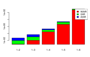
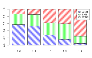
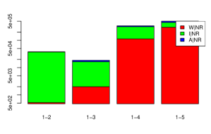
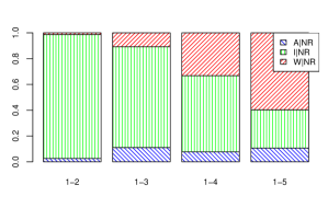
Figure 1 is a pictorial depiction of the behavior of the three search algorithms with no restarts. The chart on the left gives the absolute running time (in seconds) with a logarithmic scale. The stacked bar chart on the right reports the same data using a relative scale instead where the height of the bar is the normalized sum of the running time of all three algorithms and the length of each segment is its normalized running time. Note that, since this view is not logarithmic, adjacent bars correspond to different totals. The results clearly show that, as the difficulty of the problem increases, the quality of wdeg sharply decreases and the quality of Abs significantly improves. On the harder instances, Abs is clearly superior to Ibs and vastly outperforms wdeg. Figure 2 conveys the same information for the optimization variant with similar observations.

Table 1 gives the numerical results for instances $1-2$ to $1-6$. The first column specifies the instance, while the remaining columns report the average run times, the standard deviations, and the number of runs that did not time-out. The results are given for no-restart and slow-restart strategies for all heuristics. On the decision instance $1-6$, wdeg often fails to find a solution within the time limit and, in general, takes considerable time. Abs always finds solutions and is about 5 times faster than Ibs for the no-restart strategy which is most effective on the decision variant. On the optimization variant, wdeg cannot solve instance $1-5$ in any of the 50 runs and Ibs does not always find a solution. Abs, in contrast, finds a solution in all 50 runs well within the time limit.

In summary, on this benchmark, wdeg is vastly outperformed by Ibs and Abs as soon as the instances are not easy. Abs is clearly the most robust heuristic and produces significant improvements in performance on the most difficult instances, both in the decision and optimization variants.

Magic Square

This benchmark is also from [10] and the model is based on a direct algebraic encoding with $2\cdot n$ linear equations for the rows and columns (the square side is $n$), 2 linear equations for the diagonals, one alldifferent constraint (not enforcing domain consistency) for the entire square, $2\cdot n$ binary inequalities to order the elements in the diagonals, and two binary inequalities to order the top-left corner against the bottom-left and top-right corners. Table 2 report results for squares of size $7$ to size $10$. The $F$ column in Table 2 reports the number of successful runs (no timeout).

On magic squares, wdeg is completely dominated by Ibs and Abs: It has poor performance and is not robust even on the simpler instances. The best performance for Ibs and Abs is obtained using a fast restart, in which case Abs provides a slight improvement over Ibs. Ibs is more effective than Abs with slow or no restarts.

B	Model	$\mu_{C}$	$\mu_{T}$	$\sigma_{T}$	$F$
7	Abs$|$NR	8218.06	0.53	1.54	50
	Abs$|$R(1.1)	2094.56	0.212	0.12	50
	Abs$|$R(2)	2380.06	0.24	0.11	50
	Ibs$|$NR	1030.8	0.09	0.04	50
	Ibs$|$R(1.1)	1172.88	0.17	0.08	50
	Ibs$|$R(2)	961.78	0.11	0.05	50
	wdeg$|$NR	3294520	105.48	138.24	34
	wdeg$|$R(1.1)	4144754.2	146.25	142.82	30
	wdeg$|$R(2)	218408.26	8.03	42.77	49
8	Abs$|$NR	154783.76	7.52	42.36	49
	Abs$|$R(1.1)	5084.18	0.48	0.24	50
	Abs$|$R(2)	5941.92	0.48	0.37	50
	Ibs$|$NR	1889.4	0.21	0.16	50
	Ibs$|$R(1.1)	2694.34	0.50	0.24	50
	Ibs$|$R(2)	2524.08	0.31	0.22	50
	wdeg$|$NR	2030330.7	79.24	127.69	38
	wdeg$|$R(1.1)	644467.4	28.77	79.38	47
	wdeg$|$R(2)	339115.4	14.96	59.24	48

B	Model	$\mu_{C}$	$\mu_{T}$	$\sigma_{T}$	$F$
9	Abs$|$NR	624461.66	37.21	95.16	45
	Abs$|$R(1.1)	12273.72	0.96	0.66	50
	Abs$|$R(2)	17552.9	1.15	1.08	50
	Ibs$|$NR	630145.78	34.19	91.62	45
	Ibs$|$R(1.1)	7239.14	1.37	0.73	50
	Ibs$|$R(2)	7622.44	0.87	1.12	50
	wdeg$|$NR	5178690.7	243.38	113.08	11
	wdeg$|$R(1.1)	3588191.4	201.01	126.23	22
	wdeg$|$R(2)	1930318.7	96.67	131.75	36
10	Abs$|$NR	856210.12	55.01	111.94	42
	Abs$|$R(1.1)	32404.9	2.59	2.18	50
	Abs$|$R(2)	43621.08	3.24	5.04	50
	Ibs$|$NR	282909.94	18.50	61.00	48
	Ibs$|$R(1.1)	21936.46	3.77	2.90	50
	Ibs$|$R(2)	23336.1	2.62	3.04	50
	wdeg$|$NR	4508166.9	245.92	112.18	10
	wdeg$|$R(1.1)	-	-	-	0
	wdeg$|$R(2)	1825065.5	99.70	125.56	34

Table 2: Experimental Results on Magic Squares.

Progressive Party

The progressive party problem [12] is a constraint satisfaction problem featuring a mix of global constraint and has been used frequently for benchmarking CP, LS, and MIP solvers. The instance considered here is the $2-8$ instance with 29 guests, 8 periods and 13 hosts, i.e., 232 variables with domains of size 13. The goal is to find a schedule for a social event taking place over $k$ time periods subject to constraints on the sizes of the venues (the boats), sizes of the group, and social constraints (two groups cannot meet more than once and one group cannot go back to the same boat more than once). The model relies on multiple global alldifferent, multi-knapsacks and arithmetic constraints with reifications. This model breaks the search in $k$ phases (one per period) and uses the black-box heuristic within each period.

Row Labels	$\mu(C)$	$\mu(T)$	$\sigma(T)$	$F$
Abs$|$NR	153848.80	46.49	90.24	45
Abs$|$R(1.1)	2338.18	4.91	0.87	50
Abs$|$R(2)	4324.88	5.47	2.10	50
Ibs$|$NR	1041257.62	112.31	136.07	34
Ibs$|$R(1.1)	15357.24	5.24	2.23	50

Row Labels	$\mu(C)$	$\mu(T)$	$\sigma(T)$	$F$
Ibs$|$R(2)	60083.46	10.03	16.89	50
wdeg$|$NR	405027.32	93.91	128.18	37
wdeg$|$R(1.1)	14424.60	3.49	2.79	50
wdeg$|$R(2)	19594.12	4.00	4.50	50

Table 3: Experimental Results on the Progressive Party $2-8$.

The results are given in Table 3. Abs clearly dominates Ibs on this benchmark for all restarting strategies. Abs is also clearly superior to wdeg when no restarts are used but is slightly slower than wdeg when slow or fast restarts are used.

Nurse Rostering

This benchmark is taken from [11] and is a rostering problem assigning nurses to infants in an hospital ward, while balancing the workload. The multi-zone model can be found in Listing 1.2 in [11]. The custom search procedure is removed and replaced by a call to one of the generic searches (Ibs,Abs,wdeg). Table 4 reports the performance results for the three heuristics and 3 restarting strategies on the one-zone instances (z1-z5,z8). Note that the custom procedure in [11] relies on a dynamic-symmetry breaking on values and sophisticated variable/value ordering. Results for wdeg beyond z5 are not reported as it times out systematically. As before, column $F$ reports the number of runs that finish (out of 50), $C$ reports the number of choice points and the $T$ columns reports the mean and standard deviation of the running time.

wdeg exhibits extremely poor performance and robustness on this benchmark. Abs is clearly the most robust procedure as it solves all instances in all its runs for all the restarting strategies. It is also significantly faster than Ibs on z4 and z8. Ibs behaves well in general, except on z4 and z8 for which it sometimes fails to find solutions and takes significantly more time than Abs. It is faster than Abs on z3 and z5.

B	Model	$\mu(C)$	$\mu(T)$	$\sigma(T)$	$F$
z1	Abs$|$NR	282.12	0.02	0.00	50
	Abs$|$R(1.1)	235.52	0.02	0.01	50
	Abs$|$R(2)	267.58	0.02	0.01	50
	Ibs$|$NR	1113.26	0.07	0.01	50
	Ibs$|$R(1.1)	1028.38	0.08	0.01	50
	Ibs$|$R(2)	820.52	0.07	0.01	50
	wdeg$|$NR	45043.22	1.77	0.08	50
	wdeg$|$R(1.1)	63783.44	2.46	0.17	50
	wdeg$|$R(2)	47162.36	1.87	0.08	50
z2	Abs$|$NR	45223.02	2.42	0.65	50
	Abs$|$R(1.1)	372174.98	19.49	9.03	50
	Abs$|$R(2)	98057.72	5.03	2.53	50
	Ibs$|$NR	82182.32	3.84	0.91	50
	Ibs$|$R(1.1)	656035.56	24.86	7.60	50
	Ibs$|$R(2)	177432.42	6.78	1.96	50
	wdeg$|$NR	6361685.84	300.00	0.00	1
	wdeg$|$R(1.1)	5372380.94	300.00	0.00	3
	wdeg$|$R(2)	4944998.26	300.00	0.00	1
z3	Abs$|$NR	326902.20	23.32	10.88	50
	Abs$|$R(1.1)	1944533.10	139.55	81.15	50
	Abs$|$R(2)	488344.88	35.26	25.40	50
	Ibs$|$NR	214032.16	14.96	4.45	50
	Ibs$|$R(1.1)	893297.88	62.27	12.23	50
	Ibs$|$R(2)	287935.30	19.62	7.01	50

B	Model	$\mu(C)$	$\mu(T)$	$\sigma(T)$	$F$
z3	wdeg$|$NR	4679035.24	300.00	0.00	2
	wdeg$|$R(1.1)	5517976.00	300.00	0.00	0
	wdeg$|$R(2)	4812533.43	300.00	0.00	2
z4	Abs$|$NR	30221.04	1.41	0.09	50
	Abs$|$R(1.1)	257205.36	11.60	0.21	50
	Abs$|$R(2)	54855.60	2.53	0.08	50
	Ibs$|$NR	2794820.62	118.25	38.18	50
	Ibs$|$R(1.1)	8241949.70	300.00	0.00	2
	Ibs$|$R(2)	5817294.96	221.15	42.75	47
	wdeg$|$NR	6386541.00	300.00	0.00	0
	wdeg$|$R(1.1)	5707406.00	300.00	0.00	0
	wdeg$|$R(2)	5000897.00	300.00	0.00	0
z5	Abs$|$NR	344187.52	17.89	3.91	50
	Abs$|$R(1.1)	3899344.36	185.81	38.09	50
	Abs$|$R(2)	902142.38	43.40	12.82	50
	Ibs$|$NR	120571.44	6.16	3.61	50
	Ibs$|$R(1.1)	468481.40	24.03	18.69	50
	Ibs$|$R(2)	192116.32	9.84	5.27	50
z8	Abs$|$NR	59314.68	3.52	0.18	50
	Abs$|$R(1.1)	599777.70	36.04	3.70	50
	Abs$|$R(2)	119224.04	7.00	0.53	50
	Ibs$|$NR	7204787.00	273.18	40.34	8
	Ibs$|$R(1.1)	8201719.08	300.00	0.00	0
	Ibs$|$R(2)	4301537.08	161.61	54.71	46

Table 4: Experimental Results on Nurse Rostering.

Radiation

$B$	$\sum x\times|D(x)|$
6	1x144 + 10x37 + 296x37
7	1x178 + 10x37 + 333x37
8	1x149 + 10x37 + 333x37
9	1x175 + 10x37 + 333x37
10	1x233 + 10x50 + 441x50

Table 5: Description of the Radiation Instances.

B	Model	$\mu(C)$	$\mu(T)$	$\sigma(T)$	$F$
6	Abs$|$NR	14934.94	1.99	0.65	50
	Abs$|$R(1.1)	10653.36	1.49	0.39	50
	Abs$|$R(2)	10768.98	1.50	0.44	50
	Ibs$|$NR	65418.78	6.89	0.72	50
	Ibs$|$R(1.1)	86200.18	8.60	0.98	50
	Ibs$|$R(2)	67003.40	7.07	0.70	50
	wdeg$|$NR	23279.70	1.77	0.41	50
	wdeg$|$R(1.1)	3798.00	0.30	0.12	50
	wdeg$|$R(2)	2918.68	0.23	0.08	50
7	Abs$|$NR	17434.30	2.73	1.84	50
	Abs$|$R(1.1)	8481.62	1.53	0.35	50
	Abs$|$R(2)	9229.80	1.62	0.51	50
	Ibs$|$NR	90055.32	10.42	0.44	50
	Ibs$|$R(1.1)	161022.24	15.93	6.43	50
	Ibs$|$R(2)	98742.94	11.13	1.73	50
	wdeg$|$NR	7868.16	0.65	0.24	50
	wdeg$|$R(1.1)	2762.26	0.24	0.10	50
	wdeg$|$R(2)	2824.00	0.24	0.12	50
8	Abs$|$NR	33916.58	4.31	1.04	50
	Abs$|$R(1.1)	48638.90	6.01	0.89	50
	Abs$|$R(2)	18294.96	2.46	0.52	50
	Ibs$|$NR	84329.16	8.98	1.08	50
	Ibs$|$R(1.1)	187346.80	16.94	4.97	50

B	Model	$\mu(C)$	$\mu(T)$	$\sigma(T)$	$F$
8	Ibs$|$R(2)	88117.48	9.36	1.34	50
	wdeg$|$NR	38591.42	2.90	0.58	50
	wdeg$|$R(1.1)	20396.80	1.72	0.39	50
	wdeg$|$R(2)	6907.14	0.55	0.12	50
9	Abs$|$NR	40339.62	5.79	3.36	50
	Abs$|$R(1.1)	20599.88	3.21	0.35	50
	Abs$|$R(2)	14101.00	2.28	0.51	50
	Ibs$|$NR	85205.62	9.70	0.61	50
	Ibs$|$R(1.1)	141311.76	14.40	3.03	50
	Ibs$|$R(2)	92431.06	10.34	0.60	50
	wdeg$|$NR	90489.62	7.33	1.35	50
	wdeg$|$R(1.1)	48641.80	4.49	1.73	50
	wdeg$|$R(2)	12806.06	1.20	0.58	50
10	Abs$|$NR	210181.18	34.56	17.00	50
	Abs$|$R(1.1)	102777.38	17.19	3.53	50
	Abs$|$R(2)	50346.82	9.10	1.65	50
	Ibs$|$NR	2551543.8	300.01	0.00	0
	Ibs$|$R(1.1)	2504564.1	300.01	0.00	0
	Ibs$|$R(2)	2525199.8	300.01	0.00	0
	wdeg$|$NR	629073.46	60.09	39.47	49
	wdeg$|$R(1.1)	232572.16	27.88	2.28	50
	wdeg$|$R(2)	47175.04	5.60	1.30	50

Table 6: Experimental Results on Radiation Benchmarks.

This last benchmark is a constrained optimization problem for radiation therapy taken from the 2008 MiniZinc challenge [6]. The objective is to find a setup of a radiation therapy machine to deliver a desired radiation intensity to a tumor. The problem uses algebraic constraint and the formulation can be found in the mini-zinc repository [4]. The search procedure must deal with all the variables at once. In 2008, several solvers were unable to solve most instances in a reasonable amount of time as seen in [4], which indicates the difficulty of the instances. The instance sizes are specified in Table 5. A row gives a term for each array in the problem with its size and the size of the domains. For instance, instance 9 has one variable with domain size 175, ten variables with domain size 37, and 333 variables with domain sizes 37.

Table 6 reports the results for 5 instances. Abs clearly dominates Ibs on all instances and Ibs cannot solve the largest instance within the time limit for any restarting strategy. wdeg performs well in general on this benchmark. It is slightly faster than Abs on the largest instance for the slow and fast restarts, but is slower with no restarts. On instance 9, it is faster with no restart and slower when slow or fast restart are used. Both wdeg and Abs are effective on this problem and clearly superior to Ibs.

Summary

On this collection of benchmarks, Abs is clearly the most robust and effective heuristic. It is robust across all benchmarks and restarting strategies and is, in general, the fastest heuristic. wdeg has significant robustness and performance issues on the multi-knapsack, magic square, and nurse rostering benchmarks. Ibs has some robustness issues on radiation, some rostering instances, and the optimization variant of the large knapsack problems. It is in general significantly less efficient than Abs on the knapsack, rostering, and radiation benchmarks.

5.3 Sensitivity Analysis

Criticality of the Variable Ordering

Table 7 reports the performance of activity-based search when no value ordering is used. The value heuristic simply tries the value in increasing order as in wdeg. The results indicate that the value selection heuristic of Abs does not play a critical role and is only marginally faster/more robust on the largest instances.

B	Method	$\mu(C)$	$\mu(T)$	$\sigma(T)$	S
6	Abs$|$NR	11224.80	1.48	0.58	50
	Abs$|$R(1.1)	18803.18	2.30	0.86	50
	Abs$|$R(2)	12248.46	1.57	0.43	50
7	Abs$|$NR	7147.90	1.27	0.39	50
	Abs$|$R(1.1)	12161.34	1.92	0.68	50
	Abs$|$R(2)	10926.12	1.74	0.54	50
8	Abs$|$NR	27702.00	3.53	0.78	50
	Abs$|$R(1.1)	63755.24	7.80	2.27	50
	Abs$|$R(2)	16708.46	2.23	0.47	50

B	Method	$\mu(C)$	$\mu(T)$	$\sigma(T)$	S
9	Abs$|$NR	36534.92	5.06	1.18	50
	Abs$|$R(1.1)	46948.84	6.76	1.99	50
	Abs$|$R(2)	23600.68	3.46	1.02	50
10	Abs$|$NR	213094.82	33.70	9.23	50
	Abs$|$R(1.1)	239145.34	40.75	7.55	50
	Abs$|$R(2)	87626.36	14.87	4.14	50

Table 7: The Influence of the Value Ordering.

Sensitivity to the Sample Size

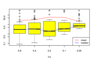
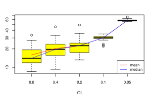
Figure 3 illustrates graphically the sensitivy of Abs to the confidence interval parameter $\delta$ used to control the number of probes in the initialization process. The statistics are based on 50 runs of the non-restarting strategy. The boxplots show the four main quartiles for the running time (in seconds) of Abs with $\delta$ ranging from 0.8 down to 0.05. The blue line connects the medians whereas the red line connects the means. The circles beyond the extreme quartiles are outliers. The left boxplot shows results on msq-10 while the right one shows results on the optimization version of knap1-4.

The results show that, as the number of probes increases (i.e., $\delta$ becomes smaller), the robustness of the search heuristic improves and the median and the mean tend to converge. This is especially true on knap1-4, while msq-10 still exhibits some variance when $\delta=0.05$. Also, the mean decreases with more probes on msq-10, while the mean increases on knap1-4 as the probe time becomes more important. The value $\delta=0.2$ used in the core experiments seem to be a reasonable compromise.

Figure 3: Sensitivity to the Sample Size as Specified by $\delta$.

Sensitivity to $\gamma$ (Aging)

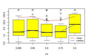
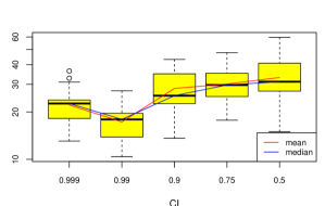
Figure 4 illustrates the sensitivity to the aging parameter. The two boxplots are once again showing the distribution of running times in seconds for 50 runs of msq-10 (left) and knap1-4 (right). What is not immediately visible on the figure is that the number of timeouts for msq-10 increases from $0$ for $\gamma=0.999$ to $9$ for $\gamma=0.5$. Overall, the results seem to indicate that the slow aging process is desirable.

Figure 4: Sensitivity to the Aging Process as Specified by $\gamma$.

5.4 Some Behavioral Observations

Figure 5 depicts the behavior of Abs and Ibs on radiation #9 under all three restarting strategies. The $x$ axis is the running time in a logarithmic scale and the $y$ axis is the objective value each time a new upper bound is found. The three red curves depict the performance of activity-based search, while the three blue curves correspond to impact-based search. What is striking here is the difference in behavior between the two searches. Abs quickly dives to the optimal solution and spends the remaining time proving optimality. Without restarts, activity-based search hits the optimum within 3 seconds. With restarts, it finds the optimal solution within one second and the proof of optimality is faster too. Ibs slowly reaches the optimal solution but then proves optimality quickly. Restarts have a negative effect on Ibs. We conjecture that the reduction of large domains may not be such a good indicator of progress and may bias the search toward certain variables.

Figure 5: The Radiation-9 Objective over Time.

Figure 6: Frequencies and Distribution of Activity Levels on Radiation-9.

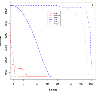
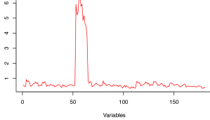
Figure 6 provide interesting data about activities on radiation #9. In particular, Figure 6 gives the frequencies of activity levels at the root, and plots the activity levels for all the variables. (Only the variables not fixed by singleton arc-consistency are shown in the figures). The two figures highlight that the probing process has isolated a small subset of the variables with very high activity levels, indicating that, on this benchmark, there are relatively few very active variables. It is tempting to conjecture that this benchmark has backdoors [14] or good cycle-cutsets [2] and that activity-based search was able to discover them, but more experiments are needed to confirm or disprove this conjecture.

6 Conclusion

Robust search procedures is a central component in the design of black-box constraint-programming solvers. This paper proposed activity-based search, the idea of using the activity of variables during propagation to guide the search. A variable activity is incremented every time the propagation step filters its domain and is aged otherwise. A sampling process is used to initialize the variable activities prior to search. Activity-based search was compared experimentally to the Ibs and wdeg heuristics on a variety of benchmarks. The experimental results have shown that Abs was significantly more robust than both Ibs and wdeg on these classes of benchmarks and often produces significant performance improvements.

References

- [1] F. Boussemart, F. Hemery, C. Lecoutre, and L. Sais. Boosting systematic search by weighting constraints. In R. L. de Mántaras and L. Saitta, editors, ECAI, pages 146–150. IOS Press, 2004.
- [2] R. Dechter and J. Pearl. The cycle-cutset method for improving search performance in ai applications. In Proceedings of IEEE conference on AI Applications, Orlando, FL, 1987.
- [3] I. Dynadec. Comet v2.1 user manual. Technical report, Providence, RI, 2009.
- [4] G12. http://www.g12.cs.mu.oz.au/minizinc/, 2008.
- [5] M. W. Moskewicz, C. F. Madigan, Y. Zhao, L. Zhang, and S. Malik. Chaff: engineering an efficient sat solver. In Proceedings of the 38th annual Design Automation Conference, DAC ’01, pages 530–535, New York, NY, USA, 2001. ACM.
- [6] N. Nethercote, P. J. Stuckey, R. Becket, S. Brand, G. J. Duck, and G. Tack. Minizinc: Towards a standard cp modelling language. In In: Proc. of 13th International Conference on Principles and Practice of Constraint Programming, pages 529–543. Springer, 2007.
- [7] L. Perron. http://code.google.com/p/or-tools/, 2010.
- [8] G. Pesant. Counting and estimating lattice points: Special polytopes for branching heuristics in constraint programming. Optima Newsletter, 81:9–14, 2009.
- [9] P. Prosser, K. Stergiou, and T. Walsh. Singleton consistencies. In CP’02, pages 353–368, London, UK, 2000. Springer-Verlag.
- [10] P. Refalo. Impact-based search strategies for constraint programming. In M. Wallace, editor, CP, volume 3258 of Lecture Notes in Computer Science, pages 557–571. Springer, 2004.
- [11] P. Schaus, P. Van Hentenryck, and J.-C. RÈgin. Scalable load balancing in nurse to patient assignment problems. In W.-J. van Hoeve and J. Hooker, editors, Integration of AI and OR Techniques in Constraint Programming for Combinatorial Optimization Problems, volume 5547 of Lecture Notes in Computer Science, pages 248–262. Springer Berlin / Heidelberg, 2009.
- [12] B. Smith, S. Brailsford, P. Hubbard, and H. Williams. The Progressive Party Problem: Integer Linear Programming and Constraint Programming Compared. Constraints, 1:119–138, 1996.
- [13] M. A. Trick. A dynamic programming approach for consistency and propagation for knapsack constraints. In Annals of Operations Research, pages 113–124, 2001.
- [14] R. Williams, C. P. Gomes, and B. Selman. Backdoors to typical case complexity. In Proceedings of the 18th international joint conference on Artificial intelligence, 1173–1178, San Francisco, CA, USA, 2003.