Iterative Algorithms for Ptychographic Phase Retrieval

Chao Yang    Jianliang Qian    Andre Schirotzek    Filipe Maia    Stefano Marchesini
Abstract

Ptychography promises diffraction limited resolution without the need for high resolution lenses. To achieve high resolution one has to solve the phase problem for many partially overlapping frames. Here we review some of the existing methods for solving ptychographic phase retrieval problem from a numerical analysis point of view, and propose alternative methods based on numerical optimization.

\definecolor

MyGrayrgb0.92,0.93,0.94

\address

Computational Research Division, Lawrence Berkeley National Laboratory, Berkeley, CA 94720. \emailcyang@lbl.gov \addressDepartment of Mathematics, Michigan State University, East Lansing, MI. \emailqian@math.msu.edu \addressAdvanced Light Source, Lawrence Berkeley National Laboratory, Berkeley, CA 94720. \emailaschirotzek@lbl.gov \addressNERSC, Lawrence Berkeley National Laboratory, Berkeley, CA 94720. \emailfrmaia@lbl.gov \addressAdvanced Light Source, Lawrence Berkeley National Laboratory, Berkeley, CA 94720. \emailsmarchesini@lbl.gov

References

  • [1] R Hegerl and W Hoppe. Dynamic theory of crystalline structure analysis by electron diffraction in inhomogeneous primary wave field. Berichte Der Bunsen-Gesellschaft Fur Physikalische Chemie, 74:1148, 1970.
  • [2] P. D. Nellist, B. C. McCallum, and J. M. Rodenburg. Resolution beyond the ’information limit’ in transmission electronmicroscopy. 374:630–632, 04 1995.
  • [3] H N Chapman. Phase-retrieval x-ray microscopy by wigner-distribution deconvolution. Ultramicroscopy, 66:153–172, 1996.
  • [4] H. M. L. Faulkner and J. M. Rodenburg. Movable aperture lensless transmission microscopy: a novel phase retrieval algorithm. Phy. Rev. Lett., 93:023903, 2004.
  • [5] J. M. Rodenburg and H. M. L. Faulkner. A phase retrieval algorithm for shifting illumination. Appl. Phy. Lett., 85:4795–4797, 2004.
  • [6] J M Rodenburg. Ptychography and related diffractive imaging methods. volume 150 of Advances in Imaging and Electron Physics, chapter Ptychography and Related Diffractive Imaging Methods, pages 87–184. Elsevier, 2008.
  • [7] M. Guizar-Sicairos and J. R. Fineup. Phase retrieval with transverse translation diversity: a nonlinear optimization approach. Opt. Express, 16:7264–7278, 2008.
  • [8] P. Thibault, M. Dierolf, O. Bunk, A. Menzel, and F. Pfeiffer. Probe retrieval in ptychographic coherent diffractive imaging. Ultramicroscopy, 109:338–343, 2009.
  • [9] J. M. Rodenburg and R. H. T. Bates. The theory of super-resolution electron microscopy via wigner-distribution deconvolution. Phil. Trans. R. Soc. Lond. A, 339:521–553, 1992.
  • [10] R. Remmert. Theory of Complex Functions. Springer-Verlag, 1991.
  • [11] K. Kreutz-Delgado. The Complex Gradient Operator and the \mathbb{CR}-Calculus. UCSD, 2003.
  • [12] T. Steihaug. The conjugate gradient method and trust regions in large scale optimization. SIAM J. Num. Anal., 20:626–637, 1983.
  • [13] S Marchesini. A unified evaluation of iterative projection algorithms for phase retrieval. Rev Sci Instrum, 78:011301, Jan 2007.
  • [14] J. Moré and D. J. Thuente. Line search algorithms with guaranteed sufficient decrease. ACM Trans. Math. Software, 20(3):286–307, 1994.
  • [15] J. Nocedal and S. J. Wright. Numerical Optimization. Springer-Verlag, New York, 1999.
  • [16] J. R. Fienup. Phase retrieval algorithms: a comparison. Appl. Opt., 21:2758–2769, 1982.
  • [17] R. Luke. Relaxed averaged alternating reflections for diffraction imaging. Inverse Problems, 21:37–50, 2005.
  • [18] S. Marchesini. Phase-retrieval and saddle-point optimization. arXiv:physics, 0611233v5:1–8, 2007.
  • [19] J. M. Rodenburg. Ptychography and related diffractive imaging methods. Advances in Imaging and Electron Physics, 150, 2008.
  • [20] C. T. Kelley. Iterative Methods for Optimization. SIAM, Philadelphia, 1999.

1 Introduction

An emerging imaging technique in X-ray science is to use a localized moving probe to collect multiple diffraction measurements of an unknown object [1, 2, 3, 4, 5, 6, 7, 8]. This technique is called “ptychography”. In a ptychography experiment, one collects a sequence of diffraction images of dimension m×m𝑚𝑚m\times m. Each image frame y𝐱(𝐫)subscript𝑦𝐱superscript𝐫y_{{\bf x}}({\bf r}^{\prime}) represents the magnitude of the Fourier transform of a(𝐫)ψ^(𝐫+𝐱)𝑎𝐫^𝜓𝐫𝐱a({\bf r})\hat{\psi}({\bf r}+{\bf x}), where a(𝐫)𝑎𝐫a({\bf r}) is a localized illumination (window) function or a probe, ψ^(𝐫)^𝜓𝐫\hat{\psi}({\bf r}) is the unknown object of interest, and 𝐱𝐱{\bf x} is a translational vector. We can express y𝐱subscript𝑦𝐱y_{{\bf x}} as

y𝐱(𝐫)=|{a(𝐫)ψ^(𝐫+𝐱)}|,subscript𝑦𝐱superscript𝐫𝑎𝐫^𝜓𝐫𝐱y_{{\bf x}}({\bf r}^{\prime})=|\mathcal{F}\{a({\bf r})\hat{\psi}({\bf r}+{\bf x})\}|, (1)

where {f}𝑓\mathcal{F}\{f\} denotes the Fourier transform of f𝑓f with respect to 𝐫𝐫{\bf r}.

In order to reconstruct the unknown object, we must retrieve the phases of the measured images. A number of methods have been proposed to recover ψ^(𝐫)^𝜓𝐫\hat{\psi}({\bf r}) from ptychographic measurements y𝐱(𝐫)subscript𝑦𝐱superscript𝐫y_{{\bf x}}({\bf r}^{\prime}) [9, 4, 5, 7, 8]. The connection among these methods is not entirely clear from the existing literature. Furthermore, little detail is provided on the convergence rate or computational efficiency of these methods.

In this paper, we review some of the existing methods for solving ptychographic phase retrieval problem from a numerical analysis point of view, and propose to solve the problem by alternative methods that are standard in the numerical optimization community. In particular, we formulate the ptychographic phase retrieval problem as an unconstrained nonlinear minimization problem in section 2, and compare the convergence of several well known iterative methods for solving this type of problem in section 6. We discuss computational details such as line search and preconditioning that are important for achieving optimal performance in these methods in section 2. We also describe the connection between optimization based algorithms and projection algorithms that are often discussed in the phase retrieval literature in section 4.

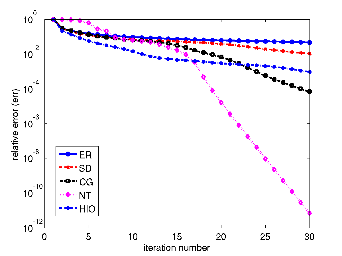
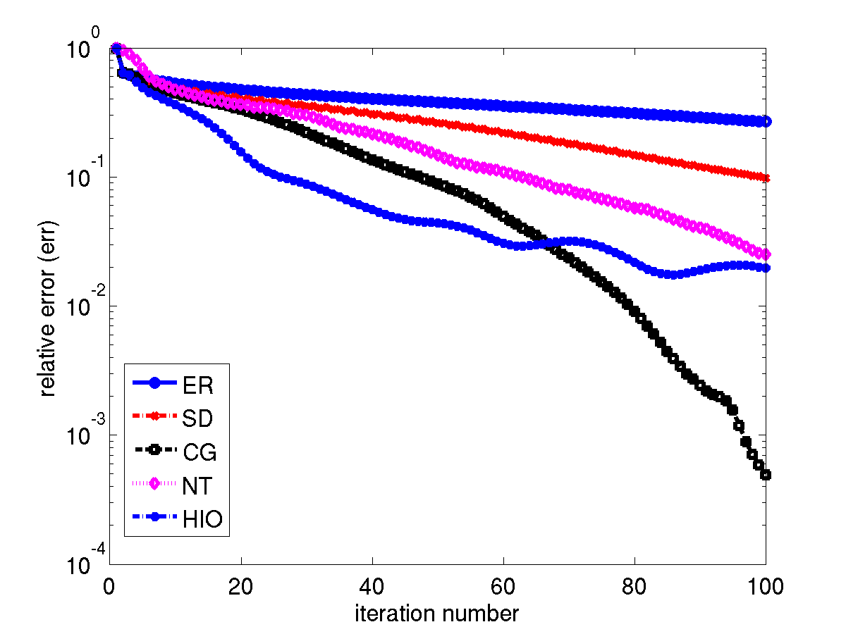
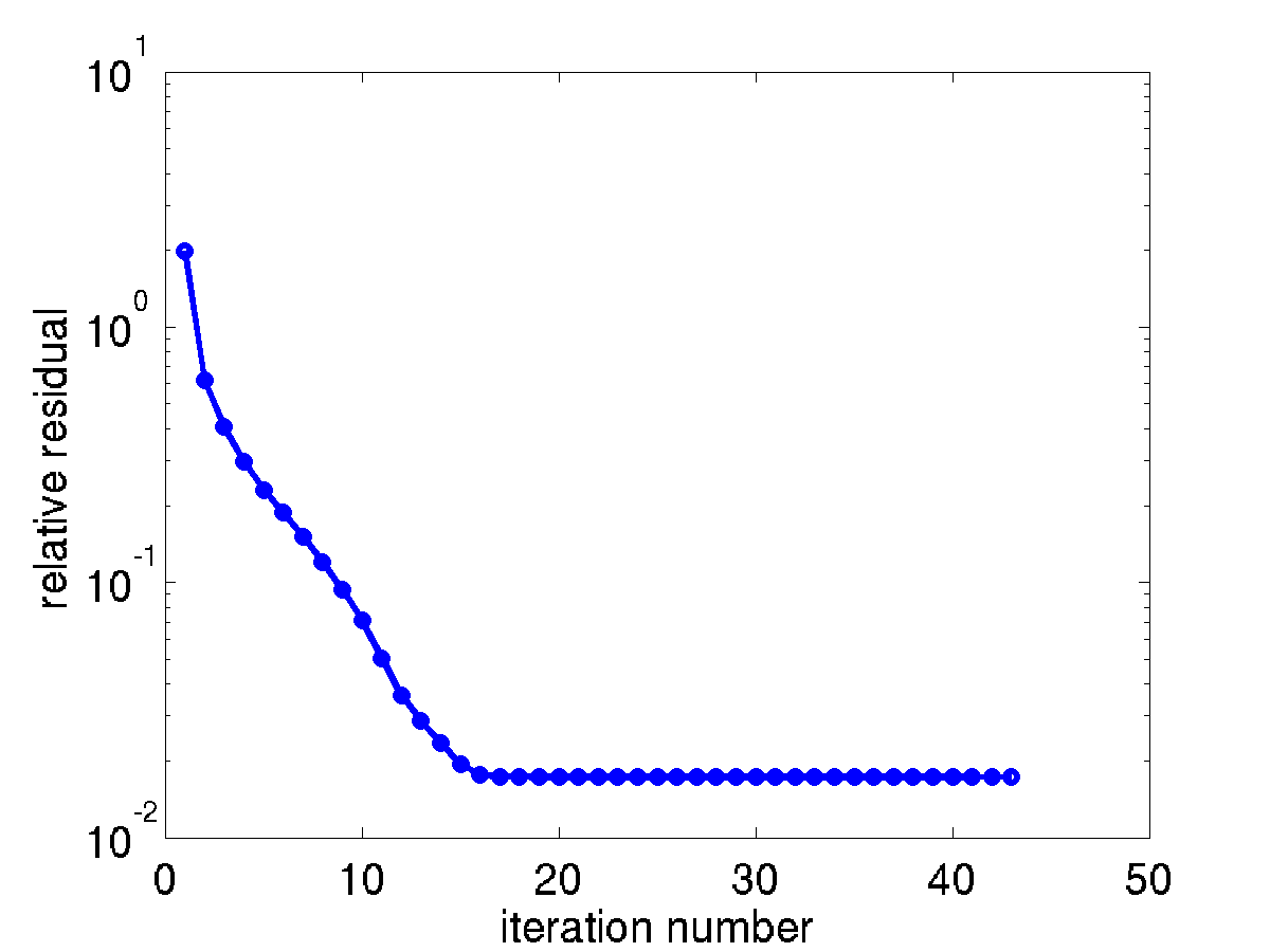
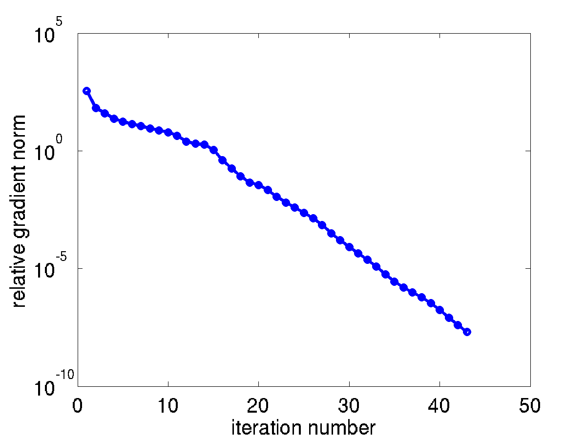
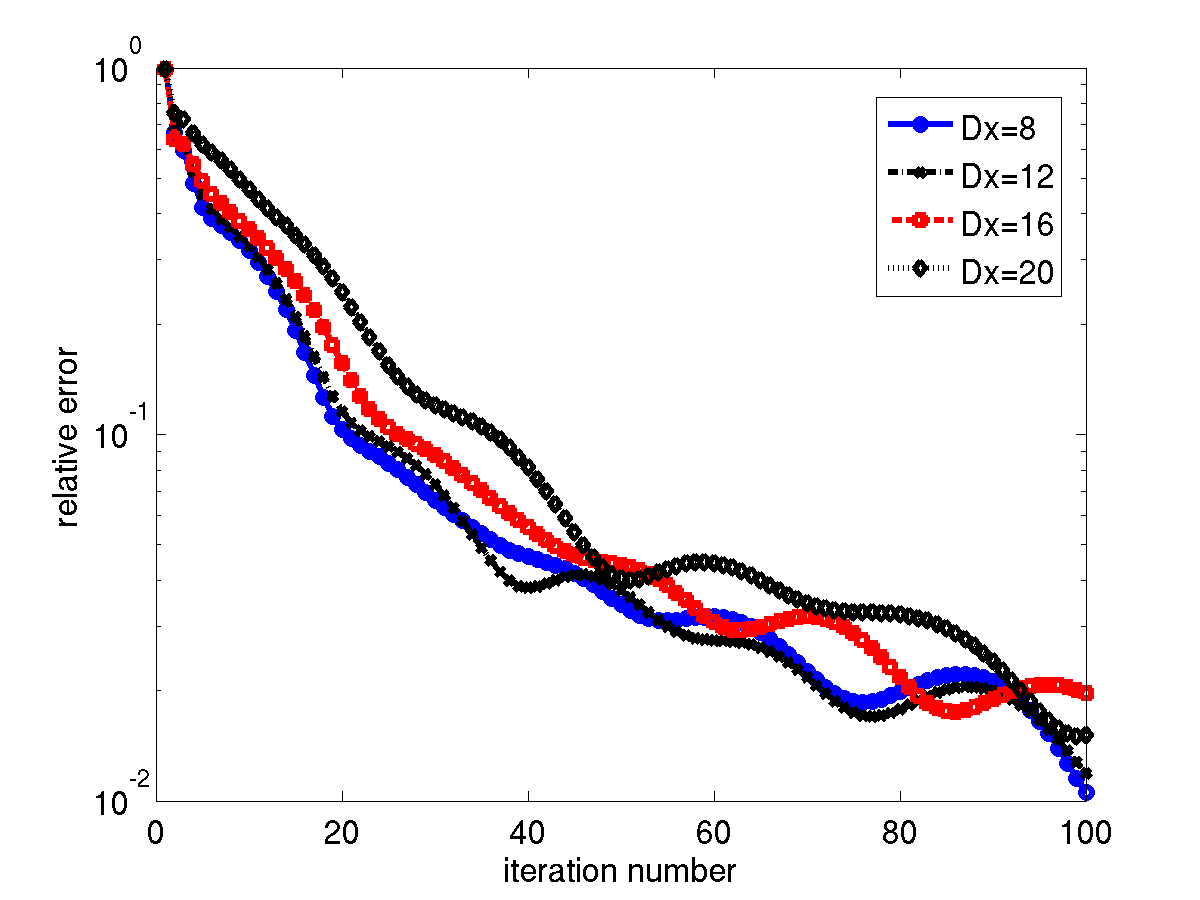
We point out that ptychographic minimization problem is not globally convex, which means that iterative methods can be trapped at a local minimizer if a poor starting guess is chosen. We show by a numerical example that one way to escape from a local minimizer is to switch to a different objective function in section 6.

We observed that the convergence of the optimization based iterative algorithms used to perform ptychographic phase retrieval is accelerated when the amount of overlap between two adjacent image frames increases. We provide an intuitive explaination on why the amount of overlap between adjacent frames affects the convergence of iterative optimization algorithms in section 6.

An alternative approach for performing ptychographic phase retrieval is a method known as Wigner deconvolution. We review this approach in section 5 and point out its connection to iterative algorithms and its limitations.

We use standard linear algebra notation whenever possible to describe various quantities evaluated in the iterative algorithms we present. To simplify notation we use a/b𝑎𝑏a/b to denote an element-wise division between two vectors a𝑎a and b𝑏b. Similarly, we use ab𝑎𝑏a\cdot b to denote an element-wise multiplication of a𝑎a and b𝑏b. We also use a2superscript𝑎2a^{2} and a1/2superscript𝑎12a^{1/2} occasionally to denote the element-wise square and square root of a𝑎a respectively. The conjugate of a complex variable a𝑎a is denoted by a¯¯𝑎\bar{a}. The real part of a𝑎a is denoted by Re(a)Re𝑎\mbox{Re}(a). The conjugate transpose of a matrix (or a vector) A𝐴A is denoted by Asuperscript𝐴A^{\ast}. The |x|𝑥|x| symbol is reserved for the magnitude (or absolute value) of x𝑥x. The Euclidean norm of x𝑥x is denoted by x=xxnorm𝑥superscript𝑥𝑥\|x\|=\sqrt{x^{\ast}x}. We use Diag(x)Diag𝑥\mbox{Diag}\left(x\right) to represent a diagonal matrix with the vector x𝑥x on its diagonal.

2 Ptychographic reconstruction formulated as an optimization problem

The problem we would like to solve is to recover ψ^^𝜓\hat{\psi} from a number of intensity measurements represented by (1). For a finite set of translational vectors 𝐱isubscript𝐱𝑖{\bf x}_{i}, we will denote each measurement by

bi=|FQiψ^|,i=1,2,,k,formulae-sequencesubscript𝑏𝑖𝐹subscript𝑄𝑖^𝜓𝑖12𝑘b_{i}=|FQ_{i}\hat{\psi}|,\ \ i=1,2,...,k,

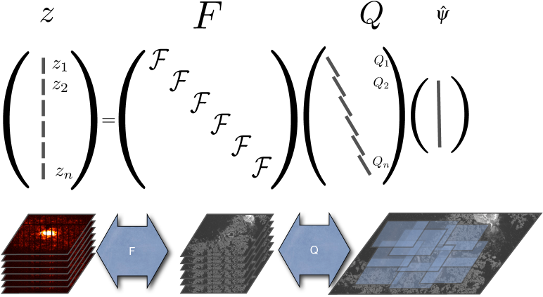
where ψ^^𝜓\hat{\psi} is the sampled unknown object that contains n𝑛n pixels, bisubscript𝑏𝑖b_{i} is a sampled measurement that contains m𝑚m pixels, F𝐹F is the matrix representation of a discrete Fourier transform, and Qisubscript𝑄𝑖Q_{i} is an m×n𝑚𝑛m\times n “illumination matrix” that extracts a frame containing m𝑚m pixels out of an image containing n𝑛n pixels. Each row of Qisubscript𝑄𝑖Q_{i} contains at most one nonzero element. The nonzero values in Qisubscript𝑄𝑖Q_{i} are determined by the illumination function a(𝐫)𝑎𝐫a({\bf r}).

Refer to caption
Figure 1: An unknown object of interest ψ^^𝜓\hat{\psi}, and the measured amplitudes zxsubscript𝑧𝑥z_{x} related by matrix operations

Given a set of measurements, b1subscript𝑏1b_{1}, b2subscript𝑏2b_{2}, …, bksubscript𝑏𝑘b_{k}, we may attempt to recover ψ^^𝜓\hat{\psi} by solving the least squares problem

minψ12i=1k|zi|bi2,subscript𝜓12superscriptsubscript𝑖1𝑘superscriptnormsubscript𝑧𝑖subscript𝑏𝑖2\min_{\psi}\frac{1}{2}\sum_{i=1}^{k}\||z_{i}|-b_{i}\|^{2}, (2)

where ziFQiψsubscript𝑧𝑖𝐹subscript𝑄𝑖𝜓z_{i}\equiv FQ_{i}\psi, and the factor of 1/2121/2 is included here merely for convenience.

An alternative objective function we may use to recover ψ^^𝜓\hat{\psi} is

ϵ=12i=1k|zi|2bi22,italic-ϵ12superscriptsubscript𝑖1𝑘superscriptnormsuperscriptsubscript𝑧𝑖2superscriptsubscript𝑏𝑖22\epsilon=\frac{1}{2}\sum_{i=1}^{k}\||z_{i}|^{2}-b_{i}^{2}\|^{2}, (3)

where |zi|2superscriptsubscript𝑧𝑖2|z_{i}|^{2} and bi2superscriptsubscript𝑏𝑖2b_{i}^{2} denote vectors obtained from squaring each component of |zi|subscript𝑧𝑖|z_{i}| and bisubscript𝑏𝑖b_{i} respectively. The advantage of using (3) is that it is more differentiable, hence more amenable to analysis. In practice, we found the objective function in (2) to be a better choice in terms of computational efficiency in most cases.

To obtain the minimizers of (2) or (3) using numerical optimization techniques, we often need to evaluate the gradient and possibly the Hessian of these objective functions. Because both (2) and (3) are real-valued functions of a (potentially) complex vector ψ𝜓\psi, derivative calculations must be done with care. One can either take the derivative of (2) and (3) with respect to the real and imaginary parts of ψ𝜓\psi independently or follow the \mathbb{CR}-calculus formalism established in [10, 11] by treating ψ𝜓\psi and ψ¯¯𝜓\bar{\psi} as two independent variables. The latter approach is what we use throughout this paper.

2.1 Gradient

If we let ri|zi|2bi2subscript𝑟𝑖superscriptsubscript𝑧𝑖2superscriptsubscript𝑏𝑖2r_{i}\equiv|z_{i}|^{2}-b_{i}^{2}, and define

r(r1r2rk),𝑟subscript𝑟1subscript𝑟2subscript𝑟𝑘r\equiv\left(\begin{array}[]{c}r_{1}\\ r_{2}\\ \vdots\\ r_{k}\end{array}\right),

we can rewrite (3) as ϵ(ψ)=rTr/2italic-ϵ𝜓superscript𝑟𝑇𝑟2\epsilon(\psi)=r^{T}r/2. Let the matrix Ji=ri/ψsubscript𝐽𝑖subscript𝑟𝑖𝜓J_{i}=\partial r_{i}/\partial\psi be the Jacobian of risubscript𝑟𝑖r_{i} with respect to ψ𝜓\psi. It follows from the chain rule that the gradient of ϵitalic-ϵ\epsilon in vector form is

ϵ(ψ)=(ϵψ)=(ϵrrψ)=Jr,italic-ϵ𝜓superscriptitalic-ϵ𝜓superscriptitalic-ϵ𝑟𝑟𝜓superscript𝐽𝑟\nabla\epsilon(\psi)=\biggl{(}\frac{\partial{\epsilon}}{\partial\psi}\biggr{)}^{\ast}=\biggl{(}\frac{\partial\epsilon}{\partial r}\frac{\partial r}{\partial\psi}\biggr{)}^{\ast}=J^{\ast}r, (4)

where

J(J1J2Jk).𝐽subscript𝐽1subscript𝐽2subscript𝐽𝑘J\equiv\left(\begin{array}[]{c}J_{1}\\ J_{2}\\ \vdots\\ J_{k}\end{array}\right).

Note that we may rewrite |zi|2superscriptsubscript𝑧𝑖2|z_{i}|^{2} as Diag(zi)ziDiagsuperscriptsubscript𝑧𝑖subscript𝑧𝑖\mbox{Diag}(z_{i})^{\ast}z_{i}, where Diag(x)Diag𝑥\mbox{Diag}(x) denotes a diagonal matrix that contains the vector x𝑥x on its diagonal and ziFQiψsubscript𝑧𝑖𝐹subscript𝑄𝑖𝜓z_{i}\equiv FQ_{i}\psi. Using this observation, we can show that

Ji=|zi|2ψ=Diag(z¯i)ziziziψ+Diag(zi)z¯iz¯iz¯iψ=Diag(z¯i)FQi=Diag(FQiψ)FQi.subscript𝐽𝑖superscriptsubscript𝑧𝑖2𝜓Diagsubscript¯𝑧𝑖subscript𝑧𝑖subscript𝑧𝑖subscript𝑧𝑖𝜓Diagsubscript𝑧𝑖subscript¯𝑧𝑖subscript¯𝑧𝑖subscript¯𝑧𝑖𝜓Diagsubscript¯𝑧𝑖𝐹subscript𝑄𝑖Diagsuperscript𝐹subscript𝑄𝑖𝜓𝐹subscript𝑄𝑖J_{i}=\frac{\partial|z_{i}|^{2}}{\partial\psi}=\frac{\partial\mbox{Diag}\left(\bar{z}_{i}\right)z_{i}}{\partial z_{i}}\frac{\partial z_{i}}{\partial\psi}+\frac{\partial\mbox{Diag}\left(z_{i}\right)\bar{z}_{i}}{\partial\bar{z}_{i}}\frac{\partial\bar{z}_{i}}{\partial\psi}=\mbox{Diag}(\bar{z}_{i})FQ_{i}=\mbox{Diag}(FQ_{i}\psi)^{\ast}FQ_{i}. (5)

It follows from (4) and the above expression that

ϵ=i=1kQiFDiag(zi)[|zi|2bi2].italic-ϵsuperscriptsubscript𝑖1𝑘superscriptsubscript𝑄𝑖superscript𝐹Diagsubscript𝑧𝑖delimited-[]superscriptsubscript𝑧𝑖2superscriptsubscript𝑏𝑖2\nabla\epsilon=\sum_{i=1}^{k}Q_{i}^{\ast}F^{\ast}\mbox{Diag}(z_{i})[|z_{i}|^{2}-b_{i}^{2}]. (6)

The gradient of the objective function in (2), which we will denote by ρ(ψ)𝜌𝜓\rho(\psi), is slightly more complicated. By rewriting |zi|subscript𝑧𝑖|z_{i}| as (|zi|2)1/2superscriptsuperscriptsubscript𝑧𝑖212(|z_{i}|^{2})^{1/2}, with the understanding that the square root is taken component-wise, and by using the chain rule and replacing |zi|2/ψsuperscriptsubscript𝑧𝑖2𝜓{\partial|z_{i}|^{2}}/{\partial\psi} with the expression given in (5), we obtain

Ji=|zi|ψ=(|zi|2)1/2|zi|2|zi|2ψ=12Diag(z¯i/|zi|)FQi,subscript𝐽𝑖subscript𝑧𝑖𝜓superscriptsuperscriptsubscript𝑧𝑖212superscriptsubscript𝑧𝑖2superscriptsubscript𝑧𝑖2𝜓12Diagsubscript¯𝑧𝑖subscript𝑧𝑖𝐹subscript𝑄𝑖J_{i}=\frac{\partial|z_{i}|}{\partial\psi}=\frac{\partial(|z_{i}|^{2})^{1/2}}{\partial|z_{i}|^{2}}\cdot\frac{\partial|z_{i}|^{2}}{\partial\psi}=\frac{1}{2}\mbox{Diag}\left(\bar{z}_{i}/|z_{i}|\right)FQ_{i},

if |zi|subscript𝑧𝑖|z_{i}| does not contain any zero element for all i=1,2,,m𝑖12𝑚i=1,2,...,m.

Consequently, we may now express ρ(ψ)𝜌𝜓\nabla\rho(\psi) as

ρ(ψ)=Jr𝜌𝜓superscript𝐽𝑟\displaystyle\nabla\rho(\psi)=J^{\ast}r =\displaystyle= i=1kJirisuperscriptsubscript𝑖1𝑘superscriptsubscript𝐽𝑖subscript𝑟𝑖\displaystyle\sum_{i=1}^{k}J_{i}^{\ast}r_{i} (7)
=\displaystyle= 12i=1kQiFDiag(zi|zi|)(|zi|bi)12superscriptsubscript𝑖1𝑘superscriptsubscript𝑄𝑖superscript𝐹Diagsubscript𝑧𝑖subscript𝑧𝑖subscript𝑧𝑖subscript𝑏𝑖\displaystyle\frac{1}{2}\sum_{i=1}^{k}Q_{i}^{\ast}F^{\ast}\mbox{Diag}\left(\frac{z_{i}}{|z_{i}|}\right)(|z_{i}|-b_{i})
=\displaystyle= 12i=1kQiF[ziDiag(zi|zi|)bi]12superscriptsubscript𝑖1𝑘superscriptsubscript𝑄𝑖superscript𝐹delimited-[]subscript𝑧𝑖Diagsubscript𝑧𝑖subscript𝑧𝑖subscript𝑏𝑖\displaystyle\frac{1}{2}\sum_{i=1}^{k}Q_{i}^{\ast}F^{\ast}\left[z_{i}-\mbox{Diag}\left(\frac{z_{i}}{|z_{i}|}\right)b_{i}\right]
=\displaystyle= 12i=1kQiF[FQiψDiag(zi|zi|)bi]12superscriptsubscript𝑖1𝑘superscriptsubscript𝑄𝑖superscript𝐹delimited-[]𝐹subscript𝑄𝑖𝜓Diagsubscript𝑧𝑖subscript𝑧𝑖subscript𝑏𝑖\displaystyle\frac{1}{2}\sum_{i=1}^{k}Q_{i}^{\ast}F^{\ast}\left[FQ_{i}\psi-\mbox{Diag}\left(\frac{z_{i}}{|z_{i}|}\right)b_{i}\right]
=\displaystyle= 12i=1k[QiQiψQiFDiag(zi|zi|)bi].12superscriptsubscript𝑖1𝑘delimited-[]superscriptsubscript𝑄𝑖subscript𝑄𝑖𝜓superscriptsubscript𝑄𝑖superscript𝐹Diagsubscript𝑧𝑖subscript𝑧𝑖subscript𝑏𝑖\displaystyle\frac{1}{2}\sum_{i=1}^{k}\left[Q_{i}^{\ast}Q_{i}\psi-Q_{i}^{\ast}F^{\ast}\mbox{Diag}\left(\frac{z_{i}}{|z_{i}|}\right)b_{i}\right].

Recall that zi=FQiψsubscript𝑧𝑖𝐹subscript𝑄𝑖𝜓z_{i}=FQ_{i}\psi. Thus, the expression Diag(FQiψ)Diag(|zi|)1biDiag𝐹subscript𝑄𝑖𝜓Diagsuperscriptsubscript𝑧𝑖1subscript𝑏𝑖\mbox{Diag}(FQ_{i}\psi)\mbox{Diag}(|z_{i}|)^{-1}b_{i} simply represents projecting ψ𝜓\psi onto the Fourier magnitude constraint imposed by the data bisubscript𝑏𝑖b_{i}. Note that the expression given above for the gradient of ρ(ψ)𝜌𝜓\rho(\psi) is only valid when |zi|subscript𝑧𝑖|z_{i}| does not contain any zero for all i=1,2,,m𝑖12𝑚i=1,2,...,m. If |zi|subscript𝑧𝑖|z_{i}| contains a zero component for some i𝑖i, and if the corresponding component in bisubscript𝑏𝑖b_{i} is nonzero, ρ𝜌\nabla\rho is not well defined, i.e., ψ𝜓\nabla\psi has singularities at ψ𝜓\psi’s where FQiψ𝐹subscript𝑄𝑖𝜓FQ_{i}\psi contains a zero element for some i𝑖i.

Note that both (6) and (7) remain real when ψ𝜓\psi is real and when bisubscript𝑏𝑖b_{i} is obtained from a discrete Fourier transform of a real image (so that conjugate symmetry is preserved in Diag(zi/|zi|)biDiagsubscript𝑧𝑖subscript𝑧𝑖subscript𝑏𝑖\mbox{Diag}\left(z_{i}/|z_{i}|\right)b_{i}.)

The directional derivatives of ϵitalic-ϵ\epsilon and ρ𝜌\rho along a direction ϕitalic-ϕ\phi are defined by

ϵψϕ+ϵψ¯ϕ¯=2i=1kRe[(|zi|2bi2)TDiag(zi)FQiϕ]italic-ϵ𝜓italic-ϕitalic-ϵ¯𝜓¯italic-ϕ2superscriptsubscript𝑖1𝑘Redelimited-[]superscriptsuperscriptsubscript𝑧𝑖2superscriptsubscript𝑏𝑖2𝑇Diagsuperscriptsubscript𝑧𝑖𝐹subscript𝑄𝑖italic-ϕ\frac{\partial\epsilon}{\partial\psi}\phi+\frac{\partial\epsilon}{\partial\bar{\psi}}\bar{\phi}=2\sum_{i=1}^{k}\mbox{Re}\biggl{[}(|z_{i}|^{2}-b_{i}^{2})^{T}\mbox{Diag}\left(z_{i}\right)^{\ast}FQ_{i}\phi\biggr{]} (8)

and

ρψϕ+ρψ¯ϕ¯=i=1kRe[ϕQiQiψϕQiFDiag(zi|zi|)bi]𝜌𝜓italic-ϕ𝜌¯𝜓¯italic-ϕsuperscriptsubscript𝑖1𝑘Redelimited-[]superscriptitalic-ϕsuperscriptsubscript𝑄𝑖subscript𝑄𝑖𝜓superscriptitalic-ϕsuperscriptsubscript𝑄𝑖superscript𝐹Diagsubscript𝑧𝑖subscript𝑧𝑖subscript𝑏𝑖\frac{\partial\rho}{\partial\psi}\phi+\frac{\partial\rho}{\partial\bar{\psi}}\bar{\phi}\\ =\sum_{i=1}^{k}\mbox{Re}\biggl{[}\phi^{\ast}Q_{i}^{\ast}Q_{i}\psi-\phi^{\ast}Q_{i}^{\ast}F^{\ast}\mbox{Diag}\left(\frac{z_{i}}{|z_{i}|}\right)b_{i}\biggr{]} (9)

respectively

2.2 Hessian

The Hessian of ϵ(ψ)italic-ϵ𝜓\epsilon(\psi) and ρ(ψ)𝜌𝜓\rho(\psi) provides information on the convexity of these objective functions. A globally convex function has a unique minimizer. Such a minimizer can be obtained by standard optimization techniques that we will describe in the next section. If the objective function is not convex everywhere, a standard optimization algorithm may produce a local minimizer that is not the true solution to ptychographic reconstruction problem.

Again, because both ϵ(ψ)italic-ϵ𝜓\epsilon(\psi) and ρ(ψ)𝜌𝜓\rho(\psi) are real valued functions of a potentially complex vector ψ𝜓\psi, their Hessians are defined as

Ho=(HψψoHψψ¯oHψ¯ψoHψ¯ψ¯o),superscript𝐻𝑜superscriptsubscript𝐻𝜓𝜓𝑜superscriptsubscript𝐻𝜓¯𝜓𝑜superscriptsubscript𝐻¯𝜓𝜓𝑜superscriptsubscript𝐻¯𝜓¯𝜓𝑜H^{o}=\left(\begin{array}[]{cc}H_{\psi\psi}^{o}&H_{\psi\bar{\psi}}^{o}\\ H_{\bar{\psi}\psi}^{o}&H_{\bar{\psi}\bar{\psi}}^{o}\end{array}\right),

where

Hψψoψ(fψ),Hψ¯ψoψ¯(fψ),Hψψ¯oψ(fψ¯),Hψ¯ψ¯oψ¯(fψ¯),formulae-sequencesuperscriptsubscript𝐻𝜓𝜓𝑜𝜓superscript𝑓𝜓formulae-sequencesuperscriptsubscript𝐻¯𝜓𝜓𝑜¯𝜓superscript𝑓𝜓formulae-sequencesuperscriptsubscript𝐻𝜓¯𝜓𝑜𝜓superscript𝑓¯𝜓superscriptsubscript𝐻¯𝜓¯𝜓𝑜¯𝜓superscript𝑓¯𝜓H_{\psi\psi}^{o}\equiv\frac{\partial}{\partial\psi}\biggl{(}\frac{\partial f}{\partial\psi}\biggr{)}^{\ast},\ \ H_{\bar{\psi}\psi}^{o}\equiv\frac{\partial}{\partial\bar{\psi}}\biggl{(}\frac{\partial f}{\partial\psi}\biggr{)}^{\ast},\ \ H_{\psi\bar{\psi}}^{o}\equiv\frac{\partial}{\partial\psi}\biggl{(}\frac{\partial f}{\partial\bar{\psi}}\biggr{)}^{\ast},\ \ H_{\bar{\psi}\bar{\psi}}^{o}\equiv\frac{\partial}{\partial\bar{\psi}}\biggl{(}\frac{\partial f}{\partial\bar{\psi}}\biggr{)}^{\ast},

and o𝑜o is either ϵitalic-ϵ\epsilon or ρ𝜌\rho.

It is not difficult to show that

Hψψϵsuperscriptsubscript𝐻𝜓𝜓italic-ϵ\displaystyle H_{\psi\psi}^{\epsilon} =\displaystyle= iQiFDiag(2|zi|2bi2)FQi,subscript𝑖superscriptsubscript𝑄𝑖superscript𝐹Diag2superscriptsubscript𝑧𝑖2superscriptsubscript𝑏𝑖2𝐹subscript𝑄𝑖\displaystyle\sum_{i}Q_{i}^{\ast}F^{\ast}\mbox{Diag}\left(2|z_{i}|^{2}-b_{i}^{2}\right)FQ_{i}, (10)
Hψ¯ψ¯ϵsuperscriptsubscript𝐻¯𝜓¯𝜓italic-ϵ\displaystyle H_{\bar{\psi}\bar{\psi}}^{\epsilon} =\displaystyle= iQiTFTDiag(2|zi|2bi2)F¯Q¯i,subscript𝑖superscriptsubscript𝑄𝑖𝑇superscript𝐹𝑇Diag2superscriptsubscript𝑧𝑖2superscriptsubscript𝑏𝑖2¯𝐹subscript¯𝑄𝑖\displaystyle\sum_{i}Q_{i}^{T}F^{T}\mbox{Diag}\left(2|z_{i}|^{2}-b_{i}^{2}\right)\bar{F}\bar{Q}_{i}, (11)
Hψψ¯ϵsuperscriptsubscript𝐻𝜓¯𝜓italic-ϵ\displaystyle H_{\psi\bar{\psi}}^{\epsilon} =\displaystyle= iQiFDiag(zi)2F¯Q¯i,subscript𝑖superscriptsubscript𝑄𝑖superscript𝐹Diagsuperscriptsubscript𝑧𝑖2¯𝐹subscript¯𝑄𝑖\displaystyle\sum_{i}Q_{i}^{\ast}F^{\ast}\mbox{Diag}\left(z_{i}\right)^{2}\bar{F}\bar{Q}_{i}, (12)
Hψ¯ψϵsuperscriptsubscript𝐻¯𝜓𝜓italic-ϵ\displaystyle H_{\bar{\psi}\psi}^{\epsilon} =\displaystyle= (Hψψ¯ϵ)=iQiTFTDiag(z¯i)2FQi.superscriptsuperscriptsubscript𝐻𝜓¯𝜓italic-ϵsubscript𝑖superscriptsubscript𝑄𝑖𝑇superscript𝐹𝑇Diagsuperscriptsubscript¯𝑧𝑖2𝐹subscript𝑄𝑖\displaystyle\left(H_{\psi\bar{\psi}}^{\epsilon}\right)^{\ast}=\sum_{i}Q_{i}^{T}F^{T}\mbox{Diag}\left(\bar{z}_{i}\right)^{2}FQ_{i}. (13)

If we let tji|tji|eiμjisubscript𝑡𝑗𝑖subscript𝑡𝑗𝑖superscript𝑒𝑖subscript𝜇𝑗𝑖t_{ji}\equiv|t_{ji}|e^{i\mu_{ji}}, ζji|ζji|eiθjisubscript𝜁𝑗𝑖subscript𝜁𝑗𝑖superscript𝑒𝑖subscript𝜃𝑗𝑖\zeta_{ji}\equiv|\zeta_{ji}|e^{i\theta_{ji}} and βjisubscript𝛽𝑗𝑖\beta_{ji} be the j𝑗jth component of ti=FQiϕsubscript𝑡𝑖𝐹subscript𝑄𝑖italic-ϕt_{i}=FQ_{i}\phi, zi=FQiψsubscript𝑧𝑖𝐹subscript𝑄𝑖𝜓z_{i}=FQ_{i}\psi and bisubscript𝑏𝑖b_{i} respectively, then the curvature τϵ(ψ,ϕ)subscript𝜏italic-ϵ𝜓italic-ϕ\tau_{\epsilon}(\psi,\phi) at ψ𝜓\psi along any direction ϕitalic-ϕ\phi can be calculated as follows

τϵ(ψ,ϕ)subscript𝜏italic-ϵ𝜓italic-ϕ\displaystyle\tau_{\epsilon}(\psi,\phi) =\displaystyle= (ϕϕT)(HψψϵHψψ¯ϵHψ¯ψϵHψ¯ψ¯ϵ)(ϕϕ¯)superscriptitalic-ϕsuperscriptitalic-ϕ𝑇superscriptsubscript𝐻𝜓𝜓italic-ϵsuperscriptsubscript𝐻𝜓¯𝜓italic-ϵsuperscriptsubscript𝐻¯𝜓𝜓italic-ϵsuperscriptsubscript𝐻¯𝜓¯𝜓italic-ϵitalic-ϕ¯italic-ϕ\displaystyle(\phi^{\ast}\ \ \phi^{T})\left(\begin{array}[]{cc}H_{\psi\psi}^{\epsilon}&H_{\psi\bar{\psi}}^{\epsilon}\\ H_{\bar{\psi}\psi}^{\epsilon}&H_{\bar{\psi}\bar{\psi}}^{\epsilon}\end{array}\right)\left(\begin{array}[]{c}\phi\\ \bar{\phi}\end{array}\right) (18)
=\displaystyle= i(titiT)(Diag(2|zi|2bi2)Diag(zi)2Diag(z¯i)2Diag(2|zi|2bi2))(titi¯)subscript𝑖superscriptsubscript𝑡𝑖superscriptsubscript𝑡𝑖𝑇Diag2superscriptsubscript𝑧𝑖2superscriptsubscript𝑏𝑖2Diagsuperscriptsubscript𝑧𝑖2Diagsuperscriptsubscript¯𝑧𝑖2Diag2superscriptsubscript𝑧𝑖2superscriptsubscript𝑏𝑖2subscript𝑡𝑖¯subscript𝑡𝑖\displaystyle\sum_{i}(t_{i}^{\ast}\ \ t_{i}^{T})\left(\begin{array}[]{cc}\mbox{Diag}\left(2|z_{i}|^{2}-b_{i}^{2}\right)&\mbox{Diag}\left(z_{i}\right)^{2}\\ \mbox{Diag}\left(\bar{z}_{i}\right)^{2}&\mbox{Diag}\left(2|z_{i}|^{2}-b_{i}^{2}\right)\end{array}\right)\left(\begin{array}[]{c}t_{i}\\ \bar{t_{i}}\end{array}\right)
=\displaystyle= i2tiDiag(2|zi|2bi2)ti+2Re[tiTDiag(z¯i)2ti]subscript𝑖2superscriptsubscript𝑡𝑖Diag2superscriptsubscript𝑧𝑖2superscriptsubscript𝑏𝑖2subscript𝑡𝑖2Redelimited-[]superscriptsubscript𝑡𝑖𝑇Diagsuperscriptsubscript¯𝑧𝑖2subscript𝑡𝑖\displaystyle\sum_{i}2t_{i}^{\ast}\mbox{Diag}\left(2|z_{i}|^{2}-b_{i}^{2}\right)t_{i}+2\mbox{Re}[t_{i}^{T}\mbox{Diag}\left(\bar{z}_{i}\right)^{2}t_{i}]
=\displaystyle= i2tiDiag(|zi|2bi2)ti+2(tiDiag(|zi|)2ti+Re[tiTDiag(z¯i)2ti])subscript𝑖2superscriptsubscript𝑡𝑖Diagsuperscriptsubscript𝑧𝑖2superscriptsubscript𝑏𝑖2subscript𝑡𝑖2superscriptsubscript𝑡𝑖Diagsuperscriptsubscript𝑧𝑖2subscript𝑡𝑖Redelimited-[]superscriptsubscript𝑡𝑖𝑇Diagsuperscriptsubscript¯𝑧𝑖2subscript𝑡𝑖\displaystyle\sum_{i}2t_{i}^{\ast}\mbox{Diag}\left(|z_{i}|^{2}-b_{i}^{2}\right)t_{i}+2\biggl{(}t_{i}^{\ast}\mbox{Diag}\left(|z_{i}|\right)^{2}t_{i}+\mbox{Re}[t_{i}^{T}\mbox{Diag}\left(\bar{z}_{i}\right)^{2}t_{i}]\biggr{)}
=\displaystyle= 2i=1kj=1n|tji|2(|zji|2βji2)+(|tji|2|zji|2+Re[(tjiz¯ji)2])2superscriptsubscript𝑖1𝑘superscriptsubscript𝑗1𝑛superscriptsubscript𝑡𝑗𝑖2superscriptsubscript𝑧𝑗𝑖2superscriptsubscript𝛽𝑗𝑖2superscriptsubscript𝑡𝑗𝑖2superscriptsubscript𝑧𝑗𝑖2Redelimited-[]superscriptsubscript𝑡𝑗𝑖subscript¯𝑧𝑗𝑖2\displaystyle 2\sum_{i=1}^{k}\sum_{j=1}^{n}|t_{ji}|^{2}(|z_{ji}|^{2}-\beta_{ji}^{2})+\biggl{(}|t_{ji}|^{2}|z_{ji}|^{2}+\mbox{Re}\biggl{[}(t_{ji}\bar{z}_{ji})^{2}\biggr{]}\biggr{)}
=\displaystyle= 2i=1kj=1n|tji|2(|zji|2βji2)+2|tji|2|zji|2cos2(μjiθji).2superscriptsubscript𝑖1𝑘superscriptsubscript𝑗1𝑛superscriptsubscript𝑡𝑗𝑖2superscriptsubscript𝑧𝑗𝑖2superscriptsubscript𝛽𝑗𝑖22superscriptsubscript𝑡𝑗𝑖2superscriptsubscript𝑧𝑗𝑖2superscript2subscript𝜇𝑗𝑖subscript𝜃𝑗𝑖\displaystyle 2\sum_{i=1}^{k}\sum_{j=1}^{n}|t_{ji}|^{2}(|z_{ji}|^{2}-\beta_{ji}^{2})+2|t_{ji}|^{2}|z_{ji}|^{2}\cos^{2}(\mu_{ji}-\theta_{ji}). (24)

At the minimizer of ϵ(ψ)italic-ϵ𝜓\epsilon(\psi), |zi|=bisubscript𝑧𝑖subscript𝑏𝑖|z_{i}|=b_{i}. So the first term of (24) is zero. Because the second term of (24) is nonnegative, τ0𝜏0\tau\geq 0, i.e., ϵitalic-ϵ\epsilon is convex at the solution. Moreover, the convexity of ϵitalic-ϵ\epsilon is preserved in the area where |zji|βjisubscript𝑧𝑗𝑖subscript𝛽𝑗𝑖|z_{ji}|\geq\beta_{ji}.

A similar observation can be made from the curvature of ρ𝜌\rho. It is not difficult to show that

Hψψρsuperscriptsubscript𝐻𝜓𝜓𝜌\displaystyle H_{\psi\psi}^{\rho} =\displaystyle= 12(i=1kQiQi12QiFDiag(bi|zi|)FQi),12superscriptsubscript𝑖1𝑘superscriptsubscript𝑄𝑖subscript𝑄𝑖12superscriptsubscript𝑄𝑖superscript𝐹Diagsubscript𝑏𝑖subscript𝑧𝑖𝐹subscript𝑄𝑖\displaystyle\frac{1}{2}\left(\sum_{i=1}^{k}Q_{i}^{\ast}Q_{i}-\frac{1}{2}Q_{i}^{\ast}F^{\ast}\mbox{Diag}\left(\frac{b_{i}}{|z_{i}|}\right)FQ_{i}\right), (25)
Hψ¯ψ¯ρsuperscriptsubscript𝐻¯𝜓¯𝜓𝜌\displaystyle H_{\bar{\psi}\bar{\psi}}^{\rho} =\displaystyle= 12(i=1kQiTQ¯i12QiTFTDiag(bi|zi|)F¯Q¯i),12superscriptsubscript𝑖1𝑘superscriptsubscript𝑄𝑖𝑇subscript¯𝑄𝑖12superscriptsubscript𝑄𝑖𝑇superscript𝐹𝑇Diagsubscript𝑏𝑖subscript𝑧𝑖¯𝐹subscript¯𝑄𝑖\displaystyle\frac{1}{2}\left(\sum_{i=1}^{k}Q_{i}^{T}\bar{Q}_{i}-\frac{1}{2}Q_{i}^{T}F^{T}\mbox{Diag}\left(\frac{b_{i}}{|z_{i}|}\right)\bar{F}\bar{Q}_{i}\right), (26)
Hψψ¯ρsuperscriptsubscript𝐻𝜓¯𝜓𝜌\displaystyle H_{\psi\bar{\psi}}^{\rho} =\displaystyle= 14i=1kQiFDiag(bizi2|zi|3)F¯Q¯i,14superscriptsubscript𝑖1𝑘superscriptsubscript𝑄𝑖superscript𝐹Diagsubscript𝑏𝑖superscriptsubscript𝑧𝑖2superscriptsubscript𝑧𝑖3¯𝐹subscript¯𝑄𝑖\displaystyle\frac{1}{4}\sum_{i=1}^{k}Q_{i}^{\ast}F^{\ast}\mbox{Diag}\left(\frac{b_{i}\cdot z_{i}^{2}}{|z_{i}|^{3}}\right)\bar{F}\bar{Q}_{i}, (27)
Hψ¯ψρsuperscriptsubscript𝐻¯𝜓𝜓𝜌\displaystyle H_{\bar{\psi}\psi}^{\rho} =\displaystyle= 14i=1kQiTFTDiag(biz¯i|zi|)FQi.14superscriptsubscript𝑖1𝑘superscriptsubscript𝑄𝑖𝑇superscript𝐹𝑇Diagsubscript𝑏𝑖subscript¯𝑧𝑖subscript𝑧𝑖𝐹subscript𝑄𝑖\displaystyle\frac{1}{4}\sum_{i=1}^{k}Q_{i}^{T}F^{T}\mbox{Diag}\left(\frac{b_{i}\cdot\bar{z}_{i}}{|z_{i}|}\right)FQ_{i}. (28)

It follows that

τρ(ψ,ϕ)subscript𝜏𝜌𝜓italic-ϕ\displaystyle\tau_{\rho}(\psi,\phi) =\displaystyle= (ϕϕT)(HψψρHψψ¯ρHψ¯ψρHψ¯ψ¯ρ)(ϕϕ¯)superscriptitalic-ϕsuperscriptitalic-ϕ𝑇superscriptsubscript𝐻𝜓𝜓𝜌superscriptsubscript𝐻𝜓¯𝜓𝜌superscriptsubscript𝐻¯𝜓𝜓𝜌superscriptsubscript𝐻¯𝜓¯𝜓𝜌italic-ϕ¯italic-ϕ\displaystyle(\phi^{\ast}\ \ \phi^{T})\left(\begin{array}[]{cc}H_{\psi\psi}^{\rho}&H_{\psi\bar{\psi}}^{\rho}\\ H_{\bar{\psi}\psi}^{\rho}&H_{\bar{\psi}\bar{\psi}}^{\rho}\end{array}\right)\left(\begin{array}[]{c}\phi\\ \bar{\phi}\end{array}\right) (33)
=\displaystyle= 12i(tit¯iT)(I12Diag(bi|zi|)12Diag(bi|zi|zi2|zi|2)12Diag(bi|zi|z¯i2|zi|2)I12Diag(bi|zi|))(tit¯i)12subscript𝑖superscriptsubscript𝑡𝑖superscriptsubscript¯𝑡𝑖𝑇𝐼12Diagsubscript𝑏𝑖subscript𝑧𝑖12Diagsubscript𝑏𝑖subscript𝑧𝑖superscriptsubscript𝑧𝑖2superscriptsubscript𝑧𝑖212Diagsubscript𝑏𝑖subscript𝑧𝑖superscriptsubscript¯𝑧𝑖2superscriptsubscript𝑧𝑖2𝐼12Diagsubscript𝑏𝑖subscript𝑧𝑖subscript𝑡𝑖subscript¯𝑡𝑖\displaystyle\frac{1}{2}\sum_{i}(t_{i}^{\ast}\ \bar{t}_{i}^{T})\left(\begin{array}[]{cc}I-\frac{1}{2}\mbox{Diag}\left(\tfrac{b_{i}}{|z_{i}|}\right)&\frac{1}{2}\mbox{Diag}\left(\tfrac{b_{i}}{|z_{i}|}\cdot\tfrac{z_{i}^{2}}{|z_{i}|^{2}}\right)\\ \frac{1}{2}\mbox{Diag}\left(\tfrac{b_{i}}{|z_{i}|}\cdot\tfrac{\bar{z}_{i}^{2}}{|z_{i}|^{2}}\right)&I-\frac{1}{2}\mbox{Diag}\left(\tfrac{b_{i}}{|z_{i}|}\right)\end{array}\right)\left(\begin{array}[]{c}t_{i}\\ \bar{t}_{i}\end{array}\right)
=\displaystyle= 12i=1kj=1n(2|tji|2|tji|2βji|ζji|+Re[t¯ji2βjiζji2|ζji|3])12superscriptsubscript𝑖1𝑘superscriptsubscript𝑗1𝑛2superscriptsubscript𝑡𝑗𝑖2superscriptsubscript𝑡𝑗𝑖2subscript𝛽𝑗𝑖subscript𝜁𝑗𝑖Redelimited-[]superscriptsubscript¯𝑡𝑗𝑖2subscript𝛽𝑗𝑖superscriptsubscript𝜁𝑗𝑖2superscriptsubscript𝜁𝑗𝑖3\displaystyle\frac{1}{2}\sum_{i=1}^{k}\sum_{j=1}^{n}\biggl{(}2|t_{ji}|^{2}-|t_{ji}|^{2}\frac{\beta_{ji}}{|\zeta_{ji}|}+\mbox{Re}\biggl{[}\bar{t}_{ji}^{2}\frac{\beta_{ji}\zeta_{ji}^{2}}{|\zeta_{ji}|^{3}}\biggr{]}\biggr{)}
=\displaystyle= 12i=1kj=1n|tji|2(2βji|ζji|+βji|ζji|Re[t¯ji2|tji|2ζji2|ζji|2])12superscriptsubscript𝑖1𝑘superscriptsubscript𝑗1𝑛superscriptsubscript𝑡𝑗𝑖22subscript𝛽𝑗𝑖subscript𝜁𝑗𝑖subscript𝛽𝑗𝑖subscript𝜁𝑗𝑖Redelimited-[]superscriptsubscript¯𝑡𝑗𝑖2superscriptsubscript𝑡𝑗𝑖2superscriptsubscript𝜁𝑗𝑖2superscriptsubscript𝜁𝑗𝑖2\displaystyle\frac{1}{2}\sum_{i=1}^{k}\sum_{j=1}^{n}|t_{ji}|^{2}\biggl{(}2-\frac{\beta_{ji}}{|\zeta_{ji}|}+\frac{\beta_{ji}}{|\zeta_{ji}|}\mbox{Re}\biggl{[}\frac{\bar{t}_{ji}^{2}}{|t_{ji}|^{2}}\frac{\zeta_{ji}^{2}}{|\zeta_{ji}|^{2}}\biggr{]}\biggr{)}
=\displaystyle= i=1kj=1n|tji|2(1βji|ζji|sin2(μjiθji)).superscriptsubscript𝑖1𝑘superscriptsubscript𝑗1𝑛superscriptsubscript𝑡𝑗𝑖21subscript𝛽𝑗𝑖subscript𝜁𝑗𝑖superscript2subscript𝜇𝑗𝑖subscript𝜃𝑗𝑖\displaystyle\sum_{i=1}^{k}\sum_{j=1}^{n}|t_{ji}|^{2}\left(1-\frac{\beta_{ji}}{|\zeta_{ji}|}\sin^{2}(\mu_{ji}-\theta_{ji})\right). (39)

Thus, τρ0subscript𝜏𝜌0\tau_{\rho}\geq 0 when |ζji|βjisubscript𝜁𝑗𝑖subscript𝛽𝑗𝑖|\zeta_{ji}|\geq\beta_{ji} for all j=1,2,,n𝑗12𝑛j=1,2,...,n and i=1,2,,k𝑖12𝑘i=1,2,...,k. Even if |ζji|subscript𝜁𝑗𝑖|\zeta_{ji}| is slightly less than βjisubscript𝛽𝑗𝑖\beta_{ji} for some j𝑗j and i𝑖i, τρsubscript𝜏𝜌\tau_{\rho} may remain positive when the corresponding sin2(μjiθji)superscript2subscript𝜇𝑗𝑖subscript𝜃𝑗𝑖\sin^{2}(\mu_{ji}-\theta_{ji}) is sufficiently small and other terms in the summation in (39) are sufficiently large and positive.

A typical problem encountered in optics is when k=1𝑘1k=1. When only one diffraction image is recorded, experience shows that local minima are common. Regions of negative curvature separate local minima from the global solution.

3 Iterative Algorithms based on Nonlinear Optimization

Because the gradient and Hessian of (2) and (3) are relatively easy to evaluate, we may use standard minimization algorithms such as the steepest descent method, the Newton’s method and the nonlinear conjugate gradient method to find the solution to the ptychographic reconstruction problem. We will review some of these methods in section 3.1 and discuss some techniques for improving the performance of these algorithms in the rest of this section.

3.1 Basic Algorithms

In many standard numerical optimization algorithms, we construct a sequence of approximations to ψ^^𝜓\hat{\psi} by

ψ(+1)=ψ()+βp(),superscript𝜓1superscript𝜓𝛽superscript𝑝\psi^{(\ell+1)}=\psi^{(\ell)}+\beta p^{(\ell)}, (40)

where p()superscript𝑝p^{(\ell)} is a search direction along which the objective function (2) or (3) decreases, and β>0𝛽0\beta>0 is an appropriate step length.

The simplest type of search direction is the steepest descent direction

psd()=ψo(ψ(),ψ¯()),superscriptsubscript𝑝sdsubscript𝜓𝑜superscript𝜓superscript¯𝜓p_{\mathrm{sd}}^{(\ell)}=-\nabla_{\psi}o(\psi^{(\ell)},\bar{\psi}^{(\ell)}),

where o𝑜o is either ϵitalic-ϵ\epsilon or ρ𝜌\rho. When the Hessian of ρ𝜌\rho or ϵitalic-ϵ\epsilon is positive definite at ψ()superscript𝜓\psi^{(\ell)}, the Newton’s direction pnt()superscriptsubscript𝑝ntp_{\mathrm{nt}}^{(\ell)}, which is the solution of

(HψψoHψψ¯oHψ¯ψoHψ¯ψ¯o)(pnt()p¯nt())=(psd()p¯sd()),superscriptsubscript𝐻𝜓𝜓𝑜superscriptsubscript𝐻𝜓¯𝜓𝑜superscriptsubscript𝐻¯𝜓𝜓𝑜superscriptsubscript𝐻¯𝜓¯𝜓𝑜superscriptsubscript𝑝ntsuperscriptsubscript¯𝑝ntsuperscriptsubscript𝑝sdsuperscriptsubscript¯𝑝sd\left(\begin{array}[]{cc}H_{\psi\psi}^{o}&H_{\psi\bar{\psi}}^{o}\\ H_{\bar{\psi}\psi}^{o}&H_{\bar{\psi}\bar{\psi}}^{o}\end{array}\right)\left(\begin{array}[]{c}p_{\mathrm{nt}}^{(\ell)}\\ \bar{p}_{\mathrm{nt}}^{(\ell)}\end{array}\right)=\left(\begin{array}[]{c}p_{\mathrm{sd}}^{(\ell)}\\ \bar{p}_{\mathrm{sd}}^{(\ell)}\end{array}\right), (41)

is also a descent direction.

Due to the nonlinear least squares nature of the objective functions (2) and (3), we may replace the true Hessian in (41) by a simpler approximation constructed from the Jacobian of the residual functions |zi|bisubscript𝑧𝑖subscript𝑏𝑖|z_{i}|-b_{i} or |zi|2bi2superscriptsubscript𝑧𝑖2superscriptsubscript𝑏𝑖2|z_{i}|^{2}-b_{i}^{2} for i=1,2,,k𝑖12𝑘i=1,2,...,k. This technique yields the Gauss-Newton (GN) search directions.

Both Newton’s method and the Gauss-Newton method require solving a system of linear equations at each step in order to obtain a search direction. Because the dimension of these linear systems is n×n𝑛𝑛n\times n, where n𝑛n is the number of pixels in the image to be reconstructed, constructing the Hessian or Jacobian and solving these equations by matrix factorization based methods will be prohibitively expensive. Iterative methods that make use of matrix vector multiplications without forming the Hessian or the J𝐽J matrix explicitly are more appropriate. However, several iterations may be required to reach a desired accuracy needed to produce a good search direction. Hence methods based on Newton or Gauss-Newton search directions tend to be more expensive.

The Hessian in (41) can also be replaced by approximations constructed from changes in the gradient computed at each iteration. Such approximation yields Quasi-Newton search directions.

Another commonly used search direction is the conjugate gradient direction defined by

pcg()=g()+αpcg(1),superscriptsubscript𝑝cgsuperscript𝑔𝛼superscriptsubscript𝑝cg1p_{\mathrm{cg}}^{(\ell)}=-g^{(\ell)}+\alpha p_{\mathrm{cg}}^{(\ell-1)},

where g()superscript𝑔g^{(\ell)} is the gradient of (2) or (3) at ψ()superscript𝜓\psi^{(\ell)} and α𝛼\alpha is often chosen to be

α=Re[(g())(g()g(1))]g(1)2.𝛼Redelimited-[]superscriptsuperscript𝑔superscript𝑔superscript𝑔1superscriptnormsuperscript𝑔12\alpha=\frac{\mbox{Re}\left[(g^{(\ell)})^{\ast}(g^{(\ell)}-g^{(\ell-1)})\right]}{\|g^{(\ell-1)}\|^{2}}.

This choice of α𝛼\alpha yields what is known as the Polak-Ribiere conjugate gradient method.

There are a variety of ways to choose an appropriate step length β𝛽\beta in (40). They are often referred to as line search methods. The purpose of line search is to ensure that the objective function decreases as we move from ψ()superscript𝜓\psi^{(\ell)} to ψ(+1)superscript𝜓1\psi^{(\ell+1)} so that ψ()superscript𝜓\psi^{(\ell)} will converge to at least a local minimizer as \ell increases. Such type of convergence is often called global convergence.

Another way to achieve global convergence in an iterative optimization procedure is to use the trust region technique to determine a search direction and step length simultaneously. Under the trust region framework, we minimize the true objective function by minimizing a sequence of simpler “surrogate” functions that mimic the behavior of the true objective function within a small neighborhood of the current approximations. That is, in each step of this iterative optimization procedure, we solve what is called a trust region subproblem

minϕΔq(ψ()+ϕ),subscriptnormitalic-ϕΔ𝑞superscript𝜓italic-ϕ\min_{\|\phi\|\leq\Delta}q(\psi^{(\ell)}+\phi), (42)

where q(ψ)𝑞𝜓q(\psi) is the surrogate function, and the parameter ΔΔ\Delta is known as a trust region radius that defines the region in which q(ψ)𝑞𝜓q(\psi) approximates ρ(ψ)𝜌𝜓\rho(\psi) or ϵ(ρ)italic-ϵ𝜌\epsilon(\rho) well. Such a radius must be chosen carefully. It may need to be adjusted iteratively based on the ratio of the reduction in the surrogate and the reduction in the true objective function achieved by the solution to (42).

A commonly used surrogate function is the second order Taylor expansion of the true objective function. The minimizer of this particular surrogate gives a full step Newton direction. However, the Newton step may not satisfy the trust region constraint, thus may not be the solution to (42).

The trust region subproblem can be solved either exactly or approximately depending on the cost of evaluating q(ψ)𝑞𝜓q(\psi) and its derivatives. If the second order Taylor expansion is chosen as the surrogate, most methods need to solve the Newton equation

2q(ϕ)s=q(ϕ),superscript2𝑞italic-ϕ𝑠𝑞italic-ϕ\nabla^{2}q(\phi)s=-\nabla q(\phi),

where 2qsuperscript2𝑞\nabla^{2}q is the Hessian of the true objective at the current iterate ψ𝜓\psi. This equation can be solved approximately by the (linear) conjugate gradient algorithm when 2superscript2\nabla^{2} is positive definite. When 2qsuperscript2𝑞\nabla^{2}q is not positive definite, (42) can also be solved by following a negative curvature direction to the boundary of the trust region. These techniques are used in an efficient iterative procedure for solving a large-scale trust region subproblem developed by Steihaug [12]. The method requires compute the matrix vector product 2qvsuperscript2𝑞𝑣\nabla^{2}qv for some vector v𝑣v. This product can be approximated by a finite difference approximation

(2q)vq(ϕ+ηv)(ϕ)η,superscript2𝑞𝑣𝑞italic-ϕ𝜂𝑣italic-ϕ𝜂(\nabla^{2}q)v\approx\frac{\nabla q(\phi+\eta v)-\nabla(\phi)}{\eta},

for some small η𝜂\eta. Therefore, it is not necessary to explicitly construct the Hessian of the objective function in Steihaug’s method.

3.2 Weighted Objective and Precondition

The least squares objective function in (2) and (3) can be expressed as

ρ(ψ)=12i=1k|zi|bi,|zi|bi,𝜌𝜓12superscriptsubscript𝑖1𝑘subscript𝑧𝑖subscript𝑏𝑖subscript𝑧𝑖subscript𝑏𝑖\rho(\psi)=\frac{1}{2}\sum_{i=1}^{k}\langle|z_{i}|-b_{i},|z_{i}|-b_{i}\rangle,

and

ϵ(ψ)=12i=1k|zi|2bi2,|zi|2bi2italic-ϵ𝜓12superscriptsubscript𝑖1𝑘superscriptsubscript𝑧𝑖2superscriptsubscript𝑏𝑖2superscriptsubscript𝑧𝑖2superscriptsubscript𝑏𝑖2\epsilon(\psi)=\frac{1}{2}\sum_{i=1}^{k}\langle|z_{i}|^{2}-b_{i}^{2},|z_{i}|^{2}-b_{i}^{2}\rangle

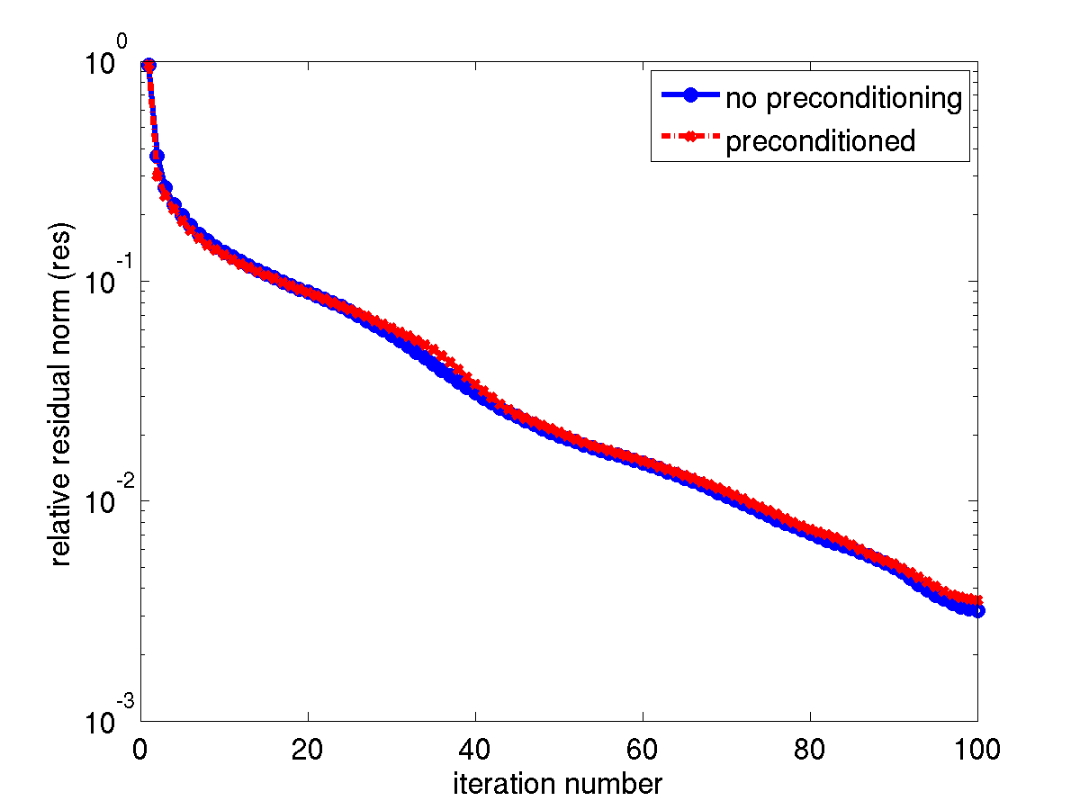
respectively, where x,y=xy𝑥𝑦superscript𝑥𝑦\langle x,y\rangle=x^{\ast}y denotes the standard Euclidean inner product. This inner product can be replaced by a weighted inner product x,yB=xBysubscript𝑥𝑦𝐵superscript𝑥𝐵𝑦\langle x,y\rangle_{B}=x^{\ast}By, where B𝐵B is a symmetric positive definite matrix, to accelerate the convergence of iterative methods used to recover the unknown image ψ𝜓\psi. As we will show in section 6, the choice of B=Diag(bi)1𝐵Diagsuperscriptsubscript𝑏𝑖1B=\mbox{Diag}(b_{i})^{-1} is particularly useful for accelerating the convergence of all iterative methods we have looked at. To maintain numerical stability and reduce noise amplification, it is often necessary to add a small constant to the diagonal of B𝐵B to prevent it from becoming singular or ill-conditioned.

Another useful technique for accelerating iterative methods for solving unconstrained minimization problem is preconditioning. Instead of minimizing ρ(ψ)𝜌𝜓\rho(\psi) or ϵ(ψ)italic-ϵ𝜓\epsilon(\psi), we make a change of variable and minimize ρ^(ϕ)^𝜌italic-ϕ\hat{\rho}(\phi) and ϵ^(ϕ)^italic-ϵitalic-ϕ\hat{\epsilon}(\phi), where ϕ=Kψitalic-ϕ𝐾𝜓\phi=K\psi, and K𝐾K is a preconditioner that is usually required to be Hermitian and positive definite. The purpose of introducing the preconditioner K𝐾K is to reduce the condition number of the Hessian of the objective function. A highly ill-conditioned Hessian often leads to slow convergence of an iterative method. A well-known example is the zig-zag behavior of the steepest descent algorithm when it is applied to the Rosenbrock function.

It follows from the chain rule and (7) that the gradient of ρ^(ψ)^𝜌𝜓\hat{\rho}(\psi) is simply

ρ^(ψ)=12K1i=1k[QiQiψQiFDiag(zi|zi|)bi],^𝜌𝜓12superscript𝐾1superscriptsubscript𝑖1𝑘delimited-[]superscriptsubscript𝑄𝑖subscript𝑄𝑖𝜓superscriptsubscript𝑄𝑖superscript𝐹Diagsubscript𝑧𝑖subscript𝑧𝑖subscript𝑏𝑖\nabla\hat{\rho}(\psi)=\frac{1}{2}K^{-1}\sum_{i=1}^{k}[Q_{i}^{\ast}Q_{i}\psi-Q_{i}^{\ast}F^{\ast}\mbox{Diag}\left(\frac{z_{i}}{|z_{i}|}\right)b_{i}],

where zi=FQiψsubscript𝑧𝑖𝐹subscript𝑄𝑖𝜓z_{i}=FQ_{i}\psi.

If we take the preconditioner to be the constant term on the diagonal blocks of Hψψρsuperscriptsubscript𝐻𝜓𝜓𝜌H_{\psi\psi}^{\rho}, i.e.,

K=i=1kQiQi,𝐾superscriptsubscript𝑖1𝑘superscriptsubscript𝑄𝑖subscript𝑄𝑖K=\sum_{i=1}^{k}Q_{i}^{\ast}Q_{i}, (43)

which is a diagonal matrix, the gradient of ρ^^𝜌\hat{\rho} simply becomes

ρ^(ψ)=12[ψ(i=1kQiQi)1(i=1kQiFDiag(zi|zi|)bi)],^𝜌𝜓12delimited-[]𝜓superscriptsuperscriptsubscript𝑖1𝑘superscriptsubscript𝑄𝑖subscript𝑄𝑖1superscriptsubscript𝑖1𝑘superscriptsubscript𝑄𝑖superscript𝐹Diagsubscript𝑧𝑖subscript𝑧𝑖subscript𝑏𝑖\nabla\hat{\rho}(\psi)=\frac{1}{2}\left[\psi-\biggl{(}\sum_{i=1}^{k}Q_{i}^{\ast}Q_{i}\biggr{)}^{-1}\biggl{(}\sum_{i=1}^{k}Q_{i}^{\ast}F^{\ast}\mbox{Diag}\left(\frac{z_{i}}{|z_{i}|}\right)b_{i}\biggr{)}\right],

and the corresponding preconditioned steepest descent algorithm with a constant step length of 2 yields the following updating formula:

ψ(+1)=(i=1kQiQi)1(i=1kQiFDiag(zi()|zi()|)bi),superscript𝜓1superscriptsuperscriptsubscript𝑖1𝑘superscriptsubscript𝑄𝑖subscript𝑄𝑖1superscriptsubscript𝑖1𝑘superscriptsubscript𝑄𝑖superscript𝐹Diagsuperscriptsubscript𝑧𝑖superscriptsubscript𝑧𝑖subscript𝑏𝑖\psi^{(\ell+1)}=\biggl{(}\sum_{i=1}^{k}Q_{i}^{\ast}Q_{i}\biggr{)}^{-1}\biggl{(}\sum_{i=1}^{k}Q_{i}^{\ast}F^{\ast}\mbox{Diag}\left(\frac{z_{i}^{(\ell)}}{|z_{i}^{(\ell)}|}\right)b_{i}\biggr{)},

where zi()=FQiψ()superscriptsubscript𝑧𝑖𝐹subscript𝑄𝑖superscript𝜓z_{i}^{(\ell)}=FQ_{i}\psi^{(\ell)}. This updating formula is identical to that used in the error reduction algorithm or alternate projection algorithm mentioned in the standard phase retrieval literature [13], which is guaranteed to converge to at least a local minimizer as shown in section 4.

3.3 Line Search

The global convergence of an unconstrained optimization algorithm depends on effective line search strategies. Assuming that ϕitalic-ϕ\phi is a descent direction for ρ(ψ)𝜌𝜓\rho(\psi) at ψ𝜓\psi, i.e., ρ(ψ)Tϕ<0𝜌superscript𝜓𝑇italic-ϕ0\nabla\rho(\psi)^{T}\phi<0, we would like to seek an appropriate step length α𝛼\alpha so that

ρ(ψ+αϕ)<ρ(ψ).𝜌𝜓𝛼italic-ϕ𝜌𝜓\rho(\psi+\alpha\phi)<\rho(\psi).

One way to obtain such a step length is to minimize the scalar function ξ(α)=ρ(ψ+αϕ)𝜉𝛼𝜌𝜓𝛼italic-ϕ\xi(\alpha)=\rho(\psi+\alpha\phi) with respect to α𝛼\alpha. This can be done by applying the Newton’s method to generate a sequence of α𝛼\alpha’s that satisfy

αi+1=αi+1ξ(αi)ξ′′(αi),subscript𝛼𝑖1subscript𝛼𝑖1superscript𝜉subscript𝛼𝑖superscript𝜉′′subscript𝛼𝑖\alpha_{i+1}=\alpha_{i+1}-\frac{\xi^{\prime}(\alpha_{i})}{\xi^{\prime\prime}(\alpha_{i})}, (44)

and accepting an αisubscript𝛼𝑖\alpha_{i} that satisfies

ξ(αi)<c1ξ(0),and|ξ(αi)|<c2|ξ(αi1)|,formulae-sequence𝜉subscript𝛼𝑖subscript𝑐1𝜉0andsuperscript𝜉subscript𝛼𝑖subscript𝑐2superscript𝜉subscript𝛼𝑖1\xi(\alpha_{i})<c_{1}\xi(0),\ \ \mbox{and}\ \ |\xi^{\prime}(\alpha_{i})|<c_{2}|\xi^{\prime}(\alpha_{i-1})|,

for some small constants 0<c1,c2<1formulae-sequence0subscript𝑐1subscript𝑐210<c_{1},c_{2}<1. In order to obtain the values of ξ(αi)superscript𝜉subscript𝛼𝑖\xi^{\prime}(\alpha_{i}) and ξ′′(αi)superscript𝜉′′subscript𝛼𝑖\xi^{\prime\prime}(\alpha_{i}) required in (44), we need to evaluate the directional derivative and curvature of ρ𝜌\rho at ψ+αiϕ𝜓subscript𝛼𝑖italic-ϕ\psi+\alpha_{i}\phi along the search direction ϕitalic-ϕ\phi. That is,

ξ(αi)superscript𝜉subscript𝛼𝑖\displaystyle\xi^{\prime}(\alpha_{i}) =\displaystyle= 2Re(ϕρ(ψ+αiϕ))2Resuperscriptitalic-ϕ𝜌𝜓subscript𝛼𝑖italic-ϕ\displaystyle 2\mbox{Re}(\phi^{\ast}\nabla\rho(\psi+\alpha_{i}\phi))
ξ′′(αi)superscript𝜉′′subscript𝛼𝑖\displaystyle\xi^{\prime\prime}(\alpha_{i}) =\displaystyle= τρ(ψ+αiϕ,ϕ).subscript𝜏𝜌𝜓subscript𝛼𝑖italic-ϕitalic-ϕ\displaystyle\tau_{\rho}(\psi+\alpha_{i}\phi,\phi).

Although these derivative calculations will incur additional computation, the cost of these computation can be kept at a minimal by keeping FQiϕ𝐹subscript𝑄𝑖italic-ϕFQ_{i}\phi in memory as we will discuss at the end of this section.

We should note that the Newton’s method may not always succeed in finding an appropriate α𝛼\alpha due to the fact that ξ(α)𝜉𝛼\xi(\alpha) is generally not globally convex. The convergence of the Newton’s method will depend on the choice of the starting guess. When a good starting guess is chosen, we typically need to run only a few Newton iterations to reach a reasonable α𝛼\alpha value. Because the purpose of line search is to identify a step length that would lead to a sufficient reduction in the objective function, it is not necessary to find the actual minimizer of ξ(α)𝜉𝛼\xi(\alpha).

However, an exact line search may not satisfy what is known as the second Wolfe condition

ρ(ψ+αϕ)pc2ρ(ψ)Tϕ,𝜌superscript𝜓𝛼italic-ϕ𝑝subscript𝑐2𝜌superscript𝜓𝑇italic-ϕ\nabla\rho(\psi+\alpha\phi)^{\ast}p\geq c_{2}\nabla\rho(\psi)^{T}\phi,

where 0<c2<10subscript𝑐210<c_{2}<1 is typically chosen to be 0.9. This condition on the change of the curvature of the objective function and the first Wolfe condition

ρ(ψ+αϕ)ρ(ψ)+c1αρ(ψ)ϕ,𝜌𝜓𝛼italic-ϕ𝜌𝜓subscript𝑐1𝛼𝜌superscript𝜓italic-ϕ\rho(\psi+\alpha\phi)\leq\rho(\psi)+c_{1}\alpha\nabla\rho(\psi)^{\ast}\phi,

for some constant c1subscript𝑐1c_{1} typically chosen to be 103superscript10310^{-3}, which is a condition that guarantees a sufficient decrease in the objective function, are required to prove the global convergence of the sequence {ψ()}superscript𝜓\{\psi^{(\ell)}\} generated by (40) in many optimization algorithms. Line search techniques that satisfy both Wolfe conditions can be found in [14] and many other standard optimization textbooks [15]. We should note that these techniques may also be sensitive to the choice of the initial guesses to the step length as well as the choice of c1subscript𝑐1c_{1} and c2subscript𝑐2c_{2} parameters. When a poor initial guess is chosen, these techniques can yield α𝛼\alpha values that are too small. Strategies for choosing a good starting guess of α𝛼\alpha can be found in [15] also.

Regardless which line search technique one uses, one typically needs to evaluate the objective function ϵ(ψ+αϕ)italic-ϵ𝜓𝛼italic-ϕ\epsilon(\psi+\alpha\phi) or ρ(ψ+αϕ)𝜌𝜓𝛼italic-ϕ\rho(\psi+\alpha\phi) and its directional derivatives for a number of different α𝛼\alpha values. If we compute ψ~=ψ+αϕ~𝜓𝜓𝛼italic-ϕ\tilde{\psi}=\psi+\alpha\phi first and use the formulae given in (2), (3), (8) and (9) to evaluate the objective function and directional derivative (by replacing ψ𝜓\psi with ψ~~𝜓\tilde{\psi}), each evaluation will perform k𝑘k FFTs. To reduce the cost of line search, we may evaluate ti=FQiϕsubscript𝑡𝑖𝐹subscript𝑄𝑖italic-ϕt_{i}=FQ_{i}\phi in advance so that no FFT is required in the the line search procedure itself. For example, to evaluate (2), we can simply compute

ρ(ψ~)=i=1k|zi+αti|bi2,𝜌~𝜓superscriptsubscript𝑖1𝑘superscriptnormsubscript𝑧𝑖𝛼subscript𝑡𝑖subscript𝑏𝑖2\rho(\tilde{\psi})=\sum_{i=1}^{k}\left\||z_{i}+\alpha t_{i}|-b_{i}\right\|^{2},

where zi=FQiψsubscript𝑧𝑖𝐹subscript𝑄𝑖𝜓z_{i}=FQ_{i}\psi and tisubscript𝑡𝑖t_{i} have been computed already. Similarly, the direction derivative of ρ𝜌\rho at ψ+αϕ𝜓𝛼italic-ϕ\psi+\alpha\phi can be obtained from

i=1kRe[ti(zi+αti)tiDiag(zi+αti|zi+αti|)bi].superscriptsubscript𝑖1𝑘Redelimited-[]superscriptsubscript𝑡𝑖subscript𝑧𝑖𝛼subscript𝑡𝑖superscriptsubscript𝑡𝑖Diagsubscript𝑧𝑖𝛼subscript𝑡𝑖subscript𝑧𝑖𝛼subscript𝑡𝑖subscript𝑏𝑖\sum_{i=1}^{k}\mbox{Re}\left[t_{i}^{\ast}(z_{i}+\alpha t_{i})-t_{i}^{\ast}\mbox{Diag}\left(\frac{z_{i}+\alpha t_{i}}{|z_{i}+\alpha t_{i}|}\right)b_{i}\right].

Also, notice that no FFT is required in the curvature calculation (39) once tisubscript𝑡𝑖t_{i}’s are available.

4 Fixed-Point Iteration and Projection Algorithms

An alternative approach to finding a minimizer of (2) is to set its gradient to zero and seek ψ𝜓\psi that satisfies the first order necessary condition of the minimization problem. If i=1kQiQisuperscriptsubscript𝑖1𝑘superscriptsubscript𝑄𝑖subscript𝑄𝑖\sum_{i=1}^{k}Q_{i}^{\ast}Q_{i} is nonsingular, by setting ρ(ψ)=12i=1k[QiQiψQiFDiag(zi|zi|)bi]𝜌𝜓12superscriptsubscript𝑖1𝑘delimited-[]superscriptsubscript𝑄𝑖subscript𝑄𝑖𝜓superscriptsubscript𝑄𝑖superscript𝐹Diagsubscript𝑧𝑖subscript𝑧𝑖subscript𝑏𝑖\nabla\rho(\psi)=\frac{1}{2}\sum_{i=1}^{k}\left[Q_{i}^{\ast}Q_{i}\psi-Q_{i}^{\ast}F^{\ast}\mbox{Diag}\left(\frac{z_{i}}{|z_{i}|}\right)b_{i}\right] to 0, we obtain

ψ=f(ψ)𝜓𝑓𝜓\psi=f(\psi) (45)

where

f(ψ)=(i=1kQiQi)1[i=1kQiFDiag(zi|zi|)bi].𝑓𝜓superscriptsuperscriptsubscript𝑖1𝑘superscriptsubscript𝑄𝑖subscript𝑄𝑖1delimited-[]superscriptsubscript𝑖1𝑘superscriptsubscript𝑄𝑖superscript𝐹Diagsubscript𝑧𝑖subscript𝑧𝑖subscript𝑏𝑖f(\psi)=\biggl{(}\sum_{i=1}^{k}Q_{i}^{\ast}Q_{i}\biggr{)}^{-1}\left[\sum_{i=1}^{k}Q_{i}^{\ast}F^{\ast}\mbox{Diag}\left(\frac{z_{i}}{|z_{i}|}\right)b_{i}\right]. (46)

Recall that ziFQiψsubscript𝑧𝑖𝐹subscript𝑄𝑖𝜓z_{i}\equiv FQ_{i}\psi. Clearly, ψ𝜓\psi is a fixed point of the function f𝑓f.

A simple iterative technique one may use to find the solution to (46) is the fixed point iteration that has the form

ψ(+1)=f(ψ()).superscript𝜓1𝑓superscript𝜓\psi^{(\ell+1)}=f(\psi^{(\ell)}).

Replacing f𝑓f with the right hand size of (46) yields

ψ(+1)=(i=1kQiQi)1[i=1kQiFDiag(zi()|zi|())bi],superscript𝜓1superscriptsuperscriptsubscript𝑖1𝑘superscriptsubscript𝑄𝑖subscript𝑄𝑖1delimited-[]superscriptsubscript𝑖1𝑘superscriptsubscript𝑄𝑖superscript𝐹Diagsuperscriptsubscript𝑧𝑖superscriptsubscript𝑧𝑖subscript𝑏𝑖\psi^{(\ell+1)}=\left(\sum_{i=1}^{k}Q_{i}^{\ast}Q_{i}\right)^{-1}\left[\sum_{i=1}^{k}Q_{i}^{\ast}F^{\ast}\mbox{Diag}\left(\frac{z_{i}^{(\ell)}}{|z_{i}|^{(\ell)}}\right)b_{i}\right], (47)

where zi()FQiψ()superscriptsubscript𝑧𝑖𝐹subscript𝑄𝑖superscript𝜓z_{i}^{(\ell)}\equiv FQ_{i}\psi^{(\ell)}. This is the same sequence of iterates produced in what is known as the error reduction algorithm in standard phase retrieval literature [13]. This method is also known as the alternate projection algorithm for reasons to be discussed below.

It is easy to verify that the updating formula in (47) is identical to that produced by a preconditioned steepest descent algorithm in which the preconditioner K𝐾K is chosen to be K=i=1kQiQi𝐾superscriptsubscript𝑖1𝑘superscriptsubscript𝑄𝑖subscript𝑄𝑖K=\sum_{i=1}^{k}Q_{i}^{\ast}Q_{i}, and a constant step length of 2 is taken at each iteration, i.e.,

ψ(+1)=ψ()2ρ(ψ()).superscript𝜓1superscript𝜓2𝜌superscript𝜓\psi^{(\ell+1)}=\psi^{(\ell)}-2\nabla\rho(\psi^{(\ell)}).

The sequence of iterates {ψ()}superscript𝜓\{\psi^{(\ell)}\} produced by (47) is guaranteed to converge to the fixed point of f(ψ)𝑓𝜓f(\psi) from any starting point {ψ(0)}superscript𝜓0\{\psi^{(0)}\}, if the spectral radius (i.e., the largest eigenvalue) of the Jacobian of f𝑓f (with respect to ψ𝜓\psi) is strictly less than 1. Because the function f𝑓f in (45) can be viewed as a function of ψ𝜓\psi and ψ¯¯𝜓\bar{\psi}, we should examine the Jacobian matrix of the system

ψ𝜓\displaystyle\psi =\displaystyle= (i=1kQiQi)1[i=1kQiFDiag(zi|zi|)bi],superscriptsuperscriptsubscript𝑖1𝑘superscriptsubscript𝑄𝑖subscript𝑄𝑖1delimited-[]superscriptsubscript𝑖1𝑘superscriptsubscript𝑄𝑖superscript𝐹Diagsubscript𝑧𝑖subscript𝑧𝑖subscript𝑏𝑖\displaystyle\left(\sum_{i=1}^{k}Q_{i}^{\ast}Q_{i}\right)^{-1}\left[\sum_{i=1}^{k}Q_{i}^{\ast}F^{\ast}\mbox{Diag}\left(\frac{z_{i}}{|z_{i}|}\right)b_{i}\right], (48)
ψ¯¯𝜓\displaystyle\bar{\psi} =\displaystyle= (i=1kQiTQ¯i)1[i=1kQiTFTDiag(z¯i|zi|)bi,]\displaystyle(\sum_{i=1}^{k}Q_{i}^{T}\bar{Q}_{i})^{-1}\left[\sum_{i=1}^{k}Q_{i}^{T}F^{T}\mbox{Diag}\left(\frac{\bar{z}_{i}}{|z_{i}|}\right)b_{i},\right] (49)

where (49) is simply the conjugate of (48). It is not difficult to show that this Jacobian matrix has the form

J=(K100K¯1)(K2Hψψρ2Hψψ¯ρ2Hψ¯ψρK¯2Hψ¯ψ¯ρ),𝐽superscript𝐾100superscript¯𝐾1𝐾2superscriptsubscript𝐻𝜓𝜓𝜌2superscriptsubscript𝐻𝜓¯𝜓𝜌2superscriptsubscript𝐻¯𝜓𝜓𝜌¯𝐾2superscriptsubscript𝐻¯𝜓¯𝜓𝜌J=\left(\begin{array}[]{cc}K^{-1}&0\\ 0&\bar{K}^{-1}\end{array}\right)\left(\begin{array}[]{cc}K-2H_{\psi\psi}^{\rho}&-2H_{\psi\bar{\psi}}^{\rho}\\ -2H_{\bar{\psi}\psi}^{\rho}&\bar{K}-2H_{\bar{\psi}\bar{\psi}}^{\rho}\end{array}\right), (50)

where Hψψρsuperscriptsubscript𝐻𝜓𝜓𝜌H_{\psi\psi}^{\rho}, Hψψ¯ρsuperscriptsubscript𝐻𝜓¯𝜓𝜌H_{\psi\bar{\psi}}^{\rho}, Hψ¯ψρsuperscriptsubscript𝐻¯𝜓𝜓𝜌H_{\bar{\psi}\psi}^{\rho} and Hψ¯ψ¯ρsuperscriptsubscript𝐻¯𝜓¯𝜓𝜌H_{\bar{\psi}\bar{\psi}}^{\rho} are as defined in (25), (27), (28) and (26) respectively.

If (λ,ϕ)𝜆italic-ϕ(\lambda,\phi) is an eigenpair of J𝐽J, we can easily show that

2(HψψρHψψ¯ρHψ¯ψρHψ¯ψ¯ρ)(ϕϕ¯)=(1λ)(K00K¯)(ϕϕ¯).2superscriptsubscript𝐻𝜓𝜓𝜌superscriptsubscript𝐻𝜓¯𝜓𝜌superscriptsubscript𝐻¯𝜓𝜓𝜌superscriptsubscript𝐻¯𝜓¯𝜓𝜌italic-ϕ¯italic-ϕ1𝜆𝐾00¯𝐾italic-ϕ¯italic-ϕ2\left(\begin{array}[]{cc}H_{\psi\psi}^{\rho}&H_{\psi\bar{\psi}}^{\rho}\\ H_{\bar{\psi}\psi}^{\rho}&H_{\bar{\psi}\bar{\psi}}^{\rho}\end{array}\right)\left(\begin{array}[]{c}\phi\\ \bar{\phi}\end{array}\right)=(1-\lambda)\left(\begin{array}[]{cc}K&0\\ 0&\bar{K}\end{array}\right)\left(\begin{array}[]{c}\phi\\ \bar{\phi}\end{array}\right).

If we again let tji|tji|eiμjisubscript𝑡𝑗𝑖subscript𝑡𝑗𝑖superscript𝑒𝑖subscript𝜇𝑗𝑖t_{ji}\equiv|t_{ji}|e^{i\mu_{ji}}, ζji|ζji|eiθjisubscript𝜁𝑗𝑖subscript𝜁𝑗𝑖superscript𝑒𝑖subscript𝜃𝑗𝑖\zeta_{ji}\equiv|\zeta_{ji}|e^{i\theta_{ji}} and βjisubscript𝛽𝑗𝑖\beta_{ji} be the j𝑗jth component of the vectors ti=FQiϕsubscript𝑡𝑖𝐹subscript𝑄𝑖italic-ϕt_{i}=FQ_{i}\phi, zi=FQiψsubscript𝑧𝑖𝐹subscript𝑄𝑖𝜓z_{i}=FQ_{i}\psi and bisubscript𝑏𝑖b_{i} respectively, we can easily show that

λ𝜆\displaystyle\lambda =\displaystyle= i=1kj=1nsin2(μjiθji)|tji|2βji/|ζji|i=1kj=1n|tji|2.superscriptsubscript𝑖1𝑘superscriptsubscript𝑗1𝑛superscript2subscript𝜇𝑗𝑖subscript𝜃𝑗𝑖superscriptsubscript𝑡𝑗𝑖2subscript𝛽𝑗𝑖subscript𝜁𝑗𝑖superscriptsubscript𝑖1𝑘superscriptsubscript𝑗1𝑛superscriptsubscript𝑡𝑗𝑖2\displaystyle\frac{\sum_{i=1}^{k}\sum_{j=1}^{n}\sin^{2}(\mu_{ji}-\theta_{ji})|t_{ji}|^{2}\beta_{ji}/|\zeta_{ji}|}{\sum_{i=1}^{k}\sum_{j=1}^{n}|t_{ji}|^{2}}. (51)

Clearly, when βji|ζji|subscript𝛽𝑗𝑖subscript𝜁𝑗𝑖\beta_{ji}\leq|\zeta_{ji}| for all j=1,2,,m𝑗12𝑚j=1,2,...,m and i=1,2,n𝑖12𝑛i=1,2,...n, |λ|1𝜆1|\lambda|\leq 1, and the fixed point iteration is guaranteed to converge to at least a local minimizer of ρ𝜌\rho.

The fixed point of f𝑓f may also be obtained by applying Newton’s algorithm to seek the root of r(ψ)=0𝑟𝜓0r(\psi)=0, where r(ψ)=ψf(ψ)𝑟𝜓𝜓𝑓𝜓r(\psi)=\psi-f(\psi). The Newton’s method produces a sequences of iterates {ψ()}superscript𝜓\{\psi^{(\ell)}\} that satisfy

ψ(+1)=ψ()J(ψ())1r(ψ()),superscript𝜓1superscript𝜓𝐽superscriptsuperscript𝜓1𝑟superscript𝜓\psi^{(\ell+1)}=\psi^{(\ell)}-J(\psi^{(\ell)})^{-1}r(\psi^{(\ell)}),

where the J𝐽J matrix here is the Jacobian of r𝑟r with respect to ψ𝜓\psi. This approach is equivalent to applying Newton’s algorithm (with appropriate line search and trust region strategies) to minimize ρ(ψ)𝜌𝜓\rho(\psi).

Successive approximations to J𝐽J can be constructed from ψ()superscript𝜓\psi^{(\ell)} and r(ψ())𝑟superscript𝜓r(\psi^{(\ell)}) using Broyden’s technique. This is similar to the Quasi-Newton algorithm discussed in the previous section. As a special case, replacing J𝐽J with the crudest approximation, the identity matrix I𝐼I, yields the standard error reduction algorithm.

If we multiply (48) from the left by Qisubscript𝑄𝑖Q_{i} for i=1,2,,k𝑖12𝑘i=1,2,...,k, and let y()=Qψ()superscript𝑦𝑄superscript𝜓y^{(\ell)}=Q\psi^{(\ell)}, where Q=(Q1Q2Qk)𝑄superscriptsuperscriptsubscript𝑄1superscriptsubscript𝑄2superscriptsubscript𝑄𝑘Q=(Q_{1}^{\ast}\ \ Q_{2}^{\ast}\ \ ...\ \ Q_{k}^{\ast})^{\ast}, we obtain

y(+1)=PQPF(y()),superscript𝑦1subscript𝑃𝑄subscript𝑃𝐹superscript𝑦y^{(\ell+1)}=P_{Q}P_{F}(y^{(\ell)}),\, (52)

where PQ=Q(QQ)1Qsubscript𝑃𝑄𝑄superscriptsuperscript𝑄𝑄1superscript𝑄P_{Q}=Q(Q^{\ast}Q)^{-1}Q^{\ast}, and

PF(y)=F^y|y|b,subscript𝑃𝐹𝑦superscript^𝐹𝑦𝑦𝑏P_{F}(y)=\hat{F}^{\ast}\frac{y}{|y|}\cdot b,

where F^=Diag(F,F,,F)^𝐹Diag𝐹𝐹𝐹\hat{F}=\mbox{Diag}\left(F,F,...,F\right) and b=(b1Tb2TbkT)T𝑏superscriptsuperscriptsubscript𝑏1𝑇superscriptsubscript𝑏2𝑇superscriptsubscript𝑏𝑘𝑇𝑇b=(b_{1}^{T}\ \ b_{2}^{T}\ \ ...\ \ b_{k}^{T})^{T}.

Because a fixed point y𝑦y of PQPFsubscript𝑃𝑄subscript𝑃𝐹P_{Q}P_{F} is in the range of Q𝑄Q, which is typically full rank when mk>n𝑚𝑘𝑛mk>n, we may recover the corresponding fixed point of f𝑓f from y𝑦y via the least squares solution ψ()=(QQ)1Qy()superscript𝜓superscriptsuperscript𝑄𝑄1superscript𝑄superscript𝑦\psi^{(\ell)}=(Q^{\ast}Q)^{-1}Q^{\ast}y^{(\ell)}.

This nonlinear map is the composition of a (linear) orthogonal projector PQsubscript𝑃𝑄P_{Q} and a (nonlinear) Fourier magnitude projector PFsubscript𝑃𝐹P_{F}. A fixed point iteration based on (52) is also called alternating projection (AP) algorithm in the phase retrieval literature because the approximation to the solution of (52) is obtained by applying PQsubscript𝑃𝑄P_{Q} and PFsubscript𝑃𝐹P_{F} in an alternating fashion.

It is easy to verify that PFsubscript𝑃𝐹P_{F} is indeed a projection operator in the sense that

PF(y)ywyfor allw{w|w=PF(w)}.formulae-sequencenormsubscript𝑃𝐹𝑦𝑦norm𝑤𝑦for all𝑤conditional-set𝑤𝑤subscript𝑃𝐹𝑤\|P_{F}(y)-y\|\leq\|w-y\|\ \ \mbox{for all}\ \ w\in\{w|w=P_{F}(w)\}. (53)

This property of PFsubscript𝑃𝐹P_{F}, together with the fact that PQsubscript𝑃𝑄P_{Q} is an orthogonal projection operator, i.e. PQyywynormsubscript𝑃𝑄𝑦𝑦norm𝑤𝑦\|P_{Q}y-y\|\leq\|w-y\| for all wRange(Q)𝑤Range𝑄w\in\mbox{Range}(Q), allows us to show that the residual error PQPF(y())y()normsubscript𝑃𝑄subscript𝑃𝐹superscript𝑦superscript𝑦\|P_{Q}P_{F}(y^{(\ell)})-y^{(\ell)}\| decreases monotonically in the AP algorithm. The proof of this observation was shown by Fienup in [16], which we summarize below.

Let y()superscript𝑦y^{(\ell)} be the vector produced in the \ell-th AP iterate. Clearly, y()Range(Q)superscript𝑦Range𝑄y^{(\ell)}\in\mbox{Range}(Q). Because PQsubscript𝑃𝑄P_{Q} is an orthogonal projector, we have

PQPF(y())PF(y())PQPF(y())y()=y(+1)y().normsubscript𝑃𝑄subscript𝑃𝐹superscript𝑦subscript𝑃𝐹superscript𝑦normsubscript𝑃𝑄subscript𝑃𝐹superscript𝑦superscript𝑦normsuperscript𝑦1superscript𝑦\|P_{Q}P_{F}(y^{(\ell)})-P_{F}(y^{(\ell)})\|\leq\|P_{Q}P_{F}(y^{(\ell)})-y^{(\ell)}\|=\|y^{(\ell+1)}-y^{(\ell)}\|. (54)

Because PF(y()){w|w=PF(w)}subscript𝑃𝐹superscript𝑦conditional-set𝑤𝑤subscript𝑃𝐹𝑤P_{F}(y^{(\ell)})\in\{w|w=P_{F}(w)\}, it follows from (53) that

PF(y(+1))y(+1)=PF(PQPF(y()))PQPF(y())PQPF(y())PF(y()).normsubscript𝑃𝐹superscript𝑦1superscript𝑦1normsubscript𝑃𝐹subscript𝑃𝑄subscript𝑃𝐹superscript𝑦subscript𝑃𝑄subscript𝑃𝐹superscript𝑦normsubscript𝑃𝑄subscript𝑃𝐹superscript𝑦subscript𝑃𝐹superscript𝑦\|P_{F}(y^{(\ell+1)})-y^{(\ell+1)}\|=\|P_{F}(P_{Q}P_{F}(y^{(\ell)}))-P_{Q}P_{F}(y^{(\ell)})\|\leq\|P_{Q}P_{F}(y^{(\ell)})-P_{F}(y^{(\ell)})\|. (55)

Consequently, we can deduce from (54) and (55) that

PF(y(+1))y(+1)y(+1)y().normsubscript𝑃𝐹superscript𝑦1superscript𝑦1normsuperscript𝑦1superscript𝑦\|P_{F}(y^{(\ell+1)})-y^{(\ell+1)}\|\leq\|y^{(\ell+1)}-y^{(\ell)}\|.

Finally, it follows from the following inequality

PQ(PF(y(+1))y(+1))PF(y(+1))y(+1),normsubscript𝑃𝑄subscript𝑃𝐹superscript𝑦1superscript𝑦1normsubscript𝑃𝐹superscript𝑦1superscript𝑦1\|P_{Q}(P_{F}(y^{(\ell+1)})-y^{(\ell+1)})\|\leq\|P_{F}(y^{(\ell+1)})-y^{(\ell+1)}\|,

and the fact that y(+1)Range(Q)superscript𝑦1Range𝑄y^{(\ell+1)}\in\mbox{Range}(Q) that

y(+2)y(+1)y(+1)y().normsuperscript𝑦2superscript𝑦1normsuperscript𝑦1superscript𝑦\|y^{(\ell+2)}-y^{(\ell+1)}\|\leq\|y^{(\ell+1)}-y^{(\ell)}\|. (56)

The equality in (56) holds only when PF(y())=y()subscript𝑃𝐹superscript𝑦superscript𝑦P_{F}(y^{(\ell)})=y^{(\ell)}, i.e., when convergence is reached.

The inequality (56) shows that the AP algorithm converges to a stationary point. However, the convergence can be extremely slow because

z(+1)=Fy(+1)=y(+1)=PQPF(y())PF(y())=b,normsuperscript𝑧1norm𝐹superscript𝑦1normsuperscript𝑦1normsubscript𝑃𝑄subscript𝑃𝐹superscript𝑦normsubscript𝑃𝐹superscript𝑦norm𝑏\|z^{(\ell+1)}\|=\|Fy^{(\ell+1)}\|=\|y^{(\ell+1)}\|=\|P_{Q}P_{F}(y^{(\ell)})\|\leq\|P_{F}(y^{(\ell)})\|=\|b\|,

and many of the terms βji/ζjisubscript𝛽𝑗𝑖subscript𝜁𝑗𝑖\beta_{ji}/\zeta_{ji}, i=1,2,,k𝑖12𝑘i=1,2,...,k and j=1,2,,m𝑗12𝑚j=1,2,...,m, in (51) may be great than 1. Only when y()superscript𝑦y^{(\ell)} is very close to the fixed point of PQPFsubscript𝑃𝑄subscript𝑃𝐹P_{Q}P_{F}, the spectral radius of the Jacobian of (46) may become much smaller than 1 in (51) due to the reduction effect of the sin2(μjiθji)superscript2subscript𝜇𝑗𝑖subscript𝜃𝑗𝑖\sin^{2}(\mu_{ji}-\theta_{ji}) terms.

The simple alternating projection algorithm has been extended to the hybrid input-output (HIO) algorithm [16], the relaxed averaged alternating reflection (RAAR) algorithm [17], and many other variants [18, 13] in the phase retrieval literature. Just to give a few examples, in the HIO and RAAR algorithms, the approximation to the solutions of (49) and (52) are updated by

y(+1)superscript𝑦1\displaystyle y^{(\ell+1)} =\displaystyle= [PQPF+(IPQ)(IβPF)]y(), HIO,delimited-[]subscript𝑃𝑄subscript𝑃𝐹𝐼subscript𝑃𝑄𝐼𝛽subscript𝑃𝐹superscript𝑦, HIO,\displaystyle\left[P_{Q}P_{F}+(I-P_{Q})(I-\beta P_{F})\right]y^{(\ell)}\text{, HIO,}
y(+1)superscript𝑦1\displaystyle y^{(\ell+1)} =\displaystyle= [2βPQPF+(12β)PF+β(PQI)]y(), RAAR.delimited-[]2𝛽subscript𝑃𝑄subscript𝑃𝐹12𝛽subscript𝑃𝐹𝛽subscript𝑃𝑄𝐼superscript𝑦, RAAR.\displaystyle\left[2\beta P_{Q}P_{F}+(1-2\beta)P_{F}+\beta(P_{Q}-I)\right]y^{(\ell)}\text{, RAAR.}
ψ(+1)superscript𝜓1\displaystyle\psi^{(\ell+1)} =\displaystyle= (QQ)1Qy(),superscriptsuperscript𝑄𝑄1superscript𝑄superscript𝑦\displaystyle(Q^{\ast}Q)^{-1}Q^{\ast}y^{(\ell)},

where β𝛽\beta is a constant often chosen to be between 0 and 1.

Although these algorithms tend to accelerate the convergence of y()superscript𝑦y^{(\ell)}, their convergence behavior is less predictable and not well understood.

5 Wigner Deconvolution

Long before iterative methods were applied to solve the ptychography problem, Rodenburg and his colleagues suggested that the problem can be solved via what they called Wigner deconvolution [9].

To explain the basic idea behind Wigner deconvolution, we need to state a continuum version of the ptychography problem. If the set of translation vectors {𝐱}𝐱\{{\bf x}\} forms a continuum in 2D, then it can be shown [19] that the Fourier transform of y𝐱2|{a(𝐫)ψ^(𝐫+𝐱)}|2superscriptsubscript𝑦𝐱2superscript𝑎𝐫^𝜓𝐫𝐱2y_{{\bf x}}^{2}\equiv|\mathcal{F}\{a({\bf r})\hat{\psi}({\bf r}+{\bf x})\}|^{2} with respect to 𝐱𝐱{\bf x}, which we denote by 𝐱{y𝐱2}subscript𝐱superscriptsubscript𝑦𝐱2\mathcal{F}_{{\bf x}}\{y_{{\bf x}}^{2}\}, can be written as the convolution of two functions with respect to 𝐫superscript𝐫{\bf r}^{\prime}, i.e.,

𝐱{y𝐱2(𝐫)}=[A(𝐫)A¯(𝐫+𝐱)]𝐫[Ψ(𝐫)Ψ¯(𝐫𝐱)],subscript𝐱superscriptsubscript𝑦𝐱2𝐫subscriptsuperscript𝐫delimited-[]𝐴superscript𝐫¯𝐴superscript𝐫superscript𝐱delimited-[]Ψsuperscript𝐫¯Ψsuperscript𝐫superscript𝐱\mathcal{F}_{{\bf x}}\{y_{{\bf x}}^{2}({\bf r})\}=[A({\bf r}^{\prime})\bar{A}({\bf r}^{\prime}+{\bf x}^{\prime})]\star_{{\bf r}^{\prime}}[\Psi({\bf r}^{\prime})\bar{\Psi}({\bf r}^{\prime}-{\bf x}^{\prime})], (57)

where A(𝐫)={a(𝐫)}𝐴superscript𝐫𝑎𝐫A({\bf r}^{\prime})=\mathcal{F}\{a({\bf r})\}, Ψ(𝐫)={ψ(𝐫)}Ψsuperscript𝐫𝜓𝐫\Psi({\bf r}^{\prime})=\mathcal{F}\{\psi({\bf r})\}, A¯¯𝐴\bar{A} denotes the conjugate of A𝐴A, Ψ¯¯Ψ\bar{\Psi} denotes the conjugate of ΨΨ\Psi, and 𝐫subscriptsuperscript𝐫\star_{{\bf r}^{\prime}} denotes a convolution operation with respect to 𝐫superscript𝐫{{\bf r}^{\prime}}. Note that 𝐱{y𝐱2(𝐫)}subscript𝐱superscriptsubscript𝑦𝐱2𝐫\mathcal{F}_{{\bf x}}\{y_{{\bf x}}^{2}({\bf r})\} is a function of 𝐱superscript𝐱{\bf x}^{\prime}. The Fourier transform of A(𝐫)A¯(𝐫+𝐱)𝐴superscript𝐫¯𝐴superscript𝐫superscript𝐱A({\bf r}^{\prime})\bar{A}({\bf r}^{\prime}+{\bf x}^{\prime}) or Ψ(𝐫)Ψ¯(𝐫𝐱)Ψsuperscript𝐫¯Ψsuperscript𝐫superscript𝐱\Psi({\bf r}^{\prime})\bar{\Psi}({\bf r}^{\prime}-{\bf x}^{\prime}) is called a Wigner distribution in [9].

The Fourier transforms used in the definition of A(𝐫)𝐴superscript𝐫A({\bf r}^{\prime}) and Ψ(𝐫)Ψsuperscript𝐫\Psi({\bf r}^{\prime}) can be replaced by discrete Fourier transforms (DFT) if both a(𝐫)𝑎𝐫a({\bf r}) and ψ(𝐫)𝜓𝐫\psi({\bf r}) are band-limited and they are sampled at or beyond the Nyquist frequency. The Fourier transform of y𝐱2superscriptsubscript𝑦𝐱2y_{{\bf x}}^{2} with respect to 𝐱𝐱{\bf x} can be replaced by a DFT only if the translation vector 𝐱𝐱{\bf x} is sampled at or beyond the Nyquist frequency of ψ(𝐫)𝜓𝐫\psi({\bf r}).

We will define a fully sampled Ψ(𝐫)Ψsuperscript𝐫\Psi({\bf r}^{\prime}) by a column vector

f=(f1f2fn)T,𝑓superscriptsubscript𝑓1subscript𝑓2subscript𝑓𝑛𝑇f=(f_{1}\>f_{2}\>\cdots f_{n})^{T},

where fi=Ψ(𝐫i)subscript𝑓𝑖Ψsubscriptsuperscript𝐫𝑖f_{i}=\Psi({\bf r}^{\prime}_{i}). Note that, when appeared by itself in ΨΨ\Psi, the variable 𝐱superscript𝐱{\bf x}^{\prime} and 𝐫superscript𝐫{\bf r}^{\prime} can be used interchangeably, i.e., fi=Ψ(𝐱i)subscript𝑓𝑖Ψsubscriptsuperscript𝐱𝑖f_{i}=\Psi({\bf x}^{\prime}_{i}) holds also.

There are at least two ways to represent Ψ(𝐫)Ψ¯(𝐫𝐱)Ψsuperscript𝐫¯Ψsuperscript𝐫superscript𝐱\Psi({\bf r}^{\prime})\bar{\Psi}({\bf r}^{\prime}-{\bf x}^{\prime}) systematically in a vector form. We choose to write it as

u(f)=(Diag(f)P1Tf¯Diag(f)P2Tf¯Diag(f)PnTf¯),𝑢𝑓Diag𝑓superscriptsubscript𝑃1𝑇¯𝑓Diag𝑓superscriptsubscript𝑃2𝑇¯𝑓Diag𝑓superscriptsubscript𝑃𝑛𝑇¯𝑓u(f)=\left(\begin{array}[]{c}\mbox{Diag}\left(f\right)P_{1}^{T}\bar{f}\\ \mbox{Diag}\left(f\right)P_{2}^{T}\bar{f}\\ \vdots\\ \mbox{Diag}\left(f\right)P_{n}^{T}\bar{f}\end{array}\right),

where Pisubscript𝑃𝑖P_{i} is a permutation matrix that shifts f¯¯𝑓\bar{f} cyclically by i1𝑖1i-1 pixels, and f¯¯𝑓\bar{f} denotes the conjugate of f𝑓f. This representation corresponds to writing down Ψ(𝐫)Ψ¯(𝐫𝐱)Ψsuperscript𝐫¯Ψsuperscript𝐫superscript𝐱\Psi({\bf r}^{\prime})\bar{\Psi}({\bf r}^{\prime}-{\bf x}^{\prime}) by having 𝐫superscript𝐫{\bf r}^{\prime} as the fastest changing index. By enumerating 𝐱superscript𝐱{\bf x}^{\prime} first, we can represent Ψ(𝐫)Ψ¯(𝐫𝐱)Ψsuperscript𝐫¯Ψsuperscript𝐫superscript𝐱\Psi({\bf r}^{\prime})\bar{\Psi}({\bf r}^{\prime}-{\bf x}^{\prime}) in an alternative form

Πu(f)=(f1P1Tf¯f2P2Tf¯fnPnTf¯),Π𝑢𝑓subscript𝑓1superscriptsubscript𝑃1𝑇¯𝑓subscript𝑓2superscriptsubscript𝑃2𝑇¯𝑓subscript𝑓𝑛superscriptsubscript𝑃𝑛𝑇¯𝑓\Pi u(f)=\left(\begin{array}[]{c}f_{1}P_{1}^{T}\bar{f}\\ f_{2}P_{2}^{T}\bar{f}\\ \vdots\\ f_{n}P_{n}^{T}\bar{f}\end{array}\right), (58)

where ΠΠ\Pi is an n2×n2superscript𝑛2superscript𝑛2n^{2}\times n^{2} permutation matrix that reorders 𝐱superscript𝐱{\bf x}^{\prime} and 𝐫superscript𝐫{\bf r}^{\prime}.

Employing the same ordering we use to represent the fully sampled Ψ(𝐫)Ψ¯(𝐫𝐱)Ψsuperscript𝐫¯Ψsuperscript𝐫superscript𝐱\Psi({\bf r}^{\prime})\bar{\Psi}({\bf r}^{\prime}-{\bf x}^{\prime}), we can express the convolution kernel A(𝐫)A(𝐫+𝐱)𝐴superscript𝐫𝐴superscript𝐫superscript𝐱A({\bf r}^{\prime})A({\bf r}^{\prime}+{\bf x}^{\prime}) by a matrix W𝑊W. This matrix has a block diagonal form, i.e.,

W=(W1W2Wn),𝑊subscript𝑊1missing-subexpressionmissing-subexpressionmissing-subexpressionmissing-subexpressionsubscript𝑊2missing-subexpressionmissing-subexpressionmissing-subexpressionmissing-subexpressionmissing-subexpressionmissing-subexpressionmissing-subexpressionmissing-subexpressionsubscript𝑊𝑛W=\left(\begin{array}[]{cccc}W_{1}&&&\\ &W_{2}&&\\ &&\ddots&\\ &&&W_{n}\end{array}\right),

where Wisubscript𝑊𝑖W_{i} is a block cyclic matrix with cyclic blocks (BCCB). This type of BCCB structure allow the convolution WiDiag(f)Pif¯subscript𝑊𝑖Diag𝑓subscript𝑃𝑖¯𝑓W_{i}\mbox{Diag}\left(f\right)P_{i}\bar{f} to be carried out efficiently by using FFTs.

Using the notation established above, we can now express the sampled version of (57) as

ΠWu(f)=b¯2,Π𝑊𝑢𝑓superscript¯𝑏2\Pi Wu(f)=\bar{b}^{2},

where

b¯2=F^Π(b12b22bm2),F^=(FFF),formulae-sequencesuperscript¯𝑏2^𝐹Πsuperscriptsubscript𝑏12superscriptsubscript𝑏22superscriptsubscript𝑏𝑚2^𝐹𝐹missing-subexpressionmissing-subexpressionmissing-subexpressionmissing-subexpression𝐹missing-subexpressionmissing-subexpressionmissing-subexpressionmissing-subexpressionmissing-subexpressionmissing-subexpressionmissing-subexpressionmissing-subexpression𝐹{\bar{b}}^{2}=\hat{F}\Pi\left(\begin{array}[]{c}b_{1}^{2}\\ b_{2}^{2}\\ \vdots\\ b_{m}^{2}\end{array}\right),\ \ \hat{F}=\left(\begin{array}[]{cccc}F&&&\\ &F&&\\ &&\ddots&\\ &&&F\end{array}\right),

and F𝐹F is the matrix representation of a 2D discrete Fourier transform of an image with n𝑛n pixels.

If W𝑊W is nonsingular, i.e., Wisubscript𝑊𝑖W_{i} is nonsingular for all i=1,2,,n𝑖12𝑛i=1,2,...,n, we can recover u(f))u(f)) by simply inverting W𝑊W, i.e.

u(f)=W1ΠTb¯2,𝑢𝑓superscript𝑊1superscriptΠ𝑇superscript¯𝑏2u(f)=W^{-1}\Pi^{T}{\bar{b}}^{2}, (59)

Equation (59) represents a deconvolution process, and is known as Wigner deconvolution [9]. The application of W1superscript𝑊1W^{-1} to the vector ΠTb¯2superscriptΠ𝑇superscript¯𝑏2\Pi^{T}{\bar{b}}^{2} can be achieved through an FFT based fast deconvolution or an iterative solver such as the conjugate gradient algorithm. We do not need to explicitly invert the matrix W𝑊W. If W𝑊W is singular or ill-conditioned, we may add a small constant to the diagonal of W𝑊W to regularize the deconvolution.

Applying the permutation ΠΠ\Pi to u(f)𝑢𝑓u(f) allows us to rewrite the solution of the deconvolution problem in the form of (58). If fi0subscript𝑓𝑖0f_{i}\neq 0 for i=1,2,,n𝑖12𝑛i=1,2,...,n, we define ci=1/fisubscript𝑐𝑖1subscript𝑓𝑖c_{i}=1/f_{i}. Furthermore, let us define g^2=ΠW1ΠTf¯2superscript^𝑔2Πsuperscript𝑊1superscriptΠ𝑇superscript¯𝑓2\hat{g}^{2}=\Pi W^{-1}\Pi^{T}{\bar{f}}^{2}, which can be partitioned as

g^2=(g^12g^22g^n2).superscript^𝑔2superscriptsubscript^𝑔12superscriptsubscript^𝑔22superscriptsubscript^𝑔𝑛2\hat{g}^{2}=\left(\begin{array}[]{c}\hat{g}_{1}^{2}\\ \hat{g}_{2}^{2}\\ \vdots\\ \hat{g}_{n}^{2}\end{array}\right).

where g^i2n×1superscriptsubscript^𝑔𝑖2superscript𝑛1\hat{g}_{i}^{2}\in\mathbb{C}^{n\times 1}.

By treating cisubscript𝑐𝑖c_{i} as a separate set of unknowns, with the exception of of c1subscript𝑐1c_{1}, which we will set to an arbitrary constant, e.g., 1, we can turn (59) into a linear least squares problem by minimizing the norm of

r=(P1TP2TDiag(g^22)PnTDiag(g^n2))(f^c2cn)(c1g^1200).𝑟superscriptsubscript𝑃1𝑇missing-subexpressionmissing-subexpressionmissing-subexpressionsuperscriptsubscript𝑃2𝑇Diagsuperscriptsubscript^𝑔22missing-subexpressionmissing-subexpressionmissing-subexpressionmissing-subexpressionsuperscriptsubscript𝑃𝑛𝑇missing-subexpressionmissing-subexpressionDiagsuperscriptsubscript^𝑔𝑛2^𝑓subscript𝑐2subscript𝑐𝑛subscript𝑐1superscriptsubscript^𝑔1200r=\left(\begin{array}[]{cccc}P_{1}^{T}&&&\\ P_{2}^{T}&-\mbox{Diag}\left(\hat{g}_{2}^{2}\right)&&\\ \vdots&&\ddots&\\ P_{n}^{T}&&&-\mbox{Diag}\left(\hat{g}_{n}^{2}\right)\\ \end{array}\right)\left(\begin{array}[]{c}\hat{f}\\ c_{2}\\ \vdots\\ c_{n}\end{array}\right)-\left(\begin{array}[]{c}c_{1}\hat{g}_{1}^{2}\\ 0\\ \vdots\\ 0\end{array}\right). (60)

The minimization of rnorm𝑟\|r\| can be easily solved by back substitution. This is essentially the “stepping out” procedure described in [9]. The reason that we can set c1subscript𝑐1c_{1} to an arbitrary constant is that we are often interested in the relative amplitudes and phases of ψ^(𝐫)^𝜓𝐫\hat{\psi}({\bf r}), multiplying the entire image ψ(𝐫)𝜓𝐫\psi({\bf r}) or Ψ(𝐫)Ψsuperscript𝐫\Psi({\bf r}^{\prime}) by a constant does not change the quality of the image.

It may seem that the use of iterative method is not necessary if we can solve the ptychography problem by Wigner deconvolution, which can be viewed as a linear inversion scheme. However, as we will show below, the Wigner deconvolution problem cannot be solved directly (using an FFT based deconvolution scheme) if 𝐱𝐱{\bf x} is sampled below the Nyquist frequency, i.e. when the amount of probe translation is larger than the resolution of the image to be reconstructed.

When 𝐱𝐱{\bf x} is sampled below the Nyquist frequency, which can occur in an experiment, we must modify (57) by introducing an aliasing operator S𝐱subscript𝑆superscript𝐱S_{{\bf x}^{\prime}}. Because a(𝐫)𝑎𝐫a({\bf r}) is a localized window in practice, A(𝐫)𝐴superscript𝐫A({\bf r}^{\prime}) is subsampled in the reciprocal space. Therefore a subsampling operator S𝐫subscript𝑆superscript𝐫S_{{\bf r}^{\prime}} must be included in a finite-dimensional analog of (57) to account for this effect.

With these additional operators, the sampled version of equation (57) can be expressed as

S𝐱ΠS𝐫Wu(f)=b¯2,subscript𝑆superscript𝐱Πsubscript𝑆superscript𝐫𝑊𝑢𝑓superscript¯𝑏2S_{{\bf x}^{\prime}}\Pi S_{{\bf r}^{\prime}}Wu(f)={\bar{b}}^{2}, (61)

where the dimensions of ΠΠ\Pi, W𝑊W, u(f)𝑢𝑓u(f) and b¯2superscript¯𝑏2{\bar{b}}^{2} need to be adjusted to reflect fewer pixel samples per diffraction frame and fewer frames resulting from increased distance 𝐱𝐱{\bf x} between two adjacent frames. For simplicity, let us assume that f𝑓f and each frame bi2superscriptsubscript𝑏𝑖2b_{i}^{2} are square images with n𝑛n and m𝑚m pixels respectively, and the distance between two adjacent frames is dxsubscript𝑑𝑥d_{x} (in either the horizontal or the vertical direction). Then, the aliasing operator S𝐱subscript𝑆superscript𝐱S_{{\bf x}^{\prime}} in (61) is a block diagonal matrix consisting of nfsubscript𝑛𝑓n_{f} diagonal blocks of dimension m×n𝑚𝑛m\times n, where nf=n/msubscript𝑛𝑓𝑛𝑚n_{f}=\lfloor\sqrt{n}/\sqrt{m}\rfloor. The subsampling operator S𝐫subscript𝑆superscript𝐫S_{{\bf r}^{\prime}} is a block diagonal matrix consisting of m𝑚m diagonal blocks of dimension nf×nsubscript𝑛𝑓𝑛n_{f}\times n, and ΠΠ\Pi is an nfm×nfmsubscript𝑛𝑓𝑚subscript𝑛𝑓𝑚n_{f}m\times n_{f}m row permutation matrix that reshuffles the rows of S𝐫Wu(f)subscript𝑆superscript𝐫𝑊𝑢𝑓S_{{\bf r}^{\prime}}Wu(f) so that 𝐱superscript𝐱{\bf x}^{\prime} is the fastest changing index. For 1D signals, a diagonal block of S𝐱subscript𝑆superscript𝐱S_{{\bf x}^{\prime}} can be represented by

(ImImIm),subscript𝐼𝑚subscript𝐼𝑚subscript𝐼𝑚(I_{m}\ \ I_{m}\ \ \cdots\ \ I_{m}),

where Imsubscript𝐼𝑚I_{m} is an m×m𝑚𝑚m\times m identity matrix. Similarly, a typical diagonal block of S𝐫subscript𝑆superscript𝐫S_{{\bf r}^{\prime}} has the form

( 0Inf 0), 0subscript𝐼subscript𝑛𝑓 0(\cdots\ \ 0\ \ I_{n_{f}}\ \ 0\ \ \cdots),

where Infsubscript𝐼subscript𝑛𝑓I_{n_{f}} is an nf×nfsubscript𝑛𝑓subscript𝑛𝑓n_{f}\times n_{f} identity matrix.

Because S𝐱subscript𝑆superscript𝐱S_{{\bf x}^{\prime}}, ΠΠ\Pi and S𝐫subscript𝑆superscript𝐫S_{{\bf r}^{\prime}} are not square matrices, we cannot obtain u(f)𝑢𝑓u(f) by simply applying the inverse of these matrices and W1superscript𝑊1W^{-1} to b¯2superscript¯𝑏2{\bar{b}}^{2}.

Instead, we must recover f𝑓f, hence the fully sampled ψ^(r)^𝜓𝑟\hat{\psi}(r), by solving the following nonlinear least squares problem

minfS𝐱ΠS𝐫Wu(f)b¯22.subscript𝑓superscriptnormsubscript𝑆superscript𝐱Πsubscript𝑆superscript𝐫𝑊𝑢𝑓superscript¯𝑏22\min_{f}\|S_{{\bf x}^{\prime}}\Pi S_{{\bf r}^{\prime}}Wu(f)-{\bar{b}}^{2}\|^{2}. (62)

It is not difficult to see that the objective function in the nonlinear least squares problem (62) is equivalent to (3). Therefore, iterative optimization techniques applied to minimize (3) can be used to solve (62) also. However, the evaluation of the objective function in (62) and its derivatives, which we will not show here, are more costly because evaluating u(f)𝑢𝑓u(f) requires at least 𝒪(n2)𝒪superscript𝑛2\mathcal{O}(n^{2}) operations, and multiplying W𝑊W with u(f)𝑢𝑓u(f) requires an additional 𝒪(n2log(n))𝒪superscript𝑛2𝑛\mathcal{O}(n^{2}\log(n)) operations. This operation count is much higher than that associated with evaluating (3), which is 𝒪(mnflog(nf)+mnf)𝒪𝑚subscript𝑛𝑓subscript𝑛𝑓𝑚subscript𝑛𝑓\mathcal{O}(mn_{f}\log(n_{f})+mn_{f}).

We should mention that, if one is interested a reconstruction of limited resolution, f~~𝑓\tilde{f}, which is a cropped version of Ψ(𝐱)Ψsuperscript𝐱\Psi(-{\bf x}^{\prime}), the objective function in (62) can be modified to become

S𝐱Π(S𝐫WS𝐫T)u~(f~)b¯22,superscriptnormsubscript𝑆superscript𝐱Πsubscript𝑆superscript𝐫𝑊superscriptsubscript𝑆superscript𝐫𝑇~𝑢~𝑓superscript¯𝑏22\|S_{{\bf x}^{\prime}}\Pi(S_{{\bf r}^{\prime}}WS_{{\bf r}^{\prime}}^{T})\tilde{u}(\tilde{f})-{\bar{b}}^{2}\|^{2},

where u~(f~)m×1~𝑢~𝑓superscript𝑚1\tilde{u}(\tilde{f})\in\mathbb{C}^{m\times 1}. Furthermore, if the translation of the frame 𝐱superscript𝐱{\bf x}^{\prime} is chosen to be commensurate with the size of each frame, e.g., x=n/msuperscript𝑥𝑛𝑚x^{\prime}=\sqrt{n/m}, then S𝐱subscript𝑆superscript𝐱S_{{\bf x}^{\prime}} becomes an identity matrix. Consequently, one may obtain u~(f~)~𝑢~𝑓\tilde{u}(\tilde{f}) (and subsequently f~~𝑓\tilde{f}) by performing a Wigner deconvolution.

6 Numerical Examples

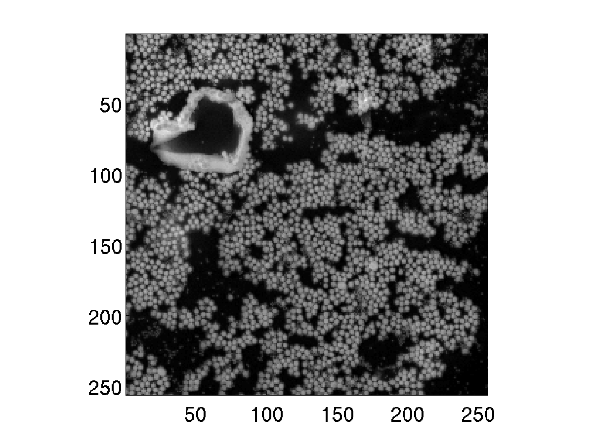
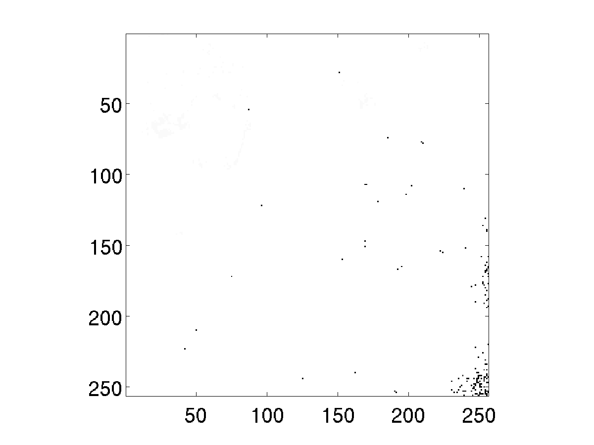
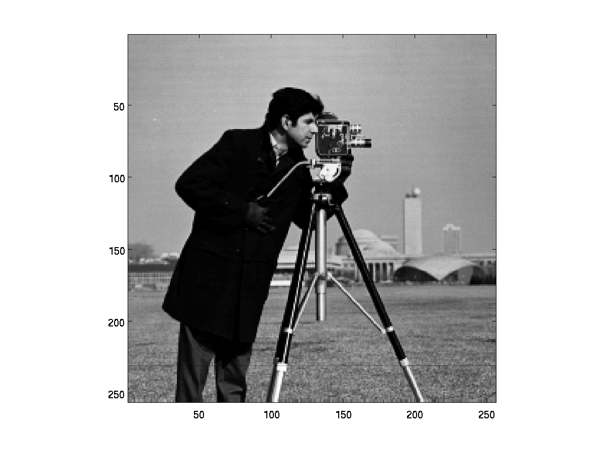
In this section, we demonstrate and compare the convergence of iterative algorithms for ptychographic reconstruction using two test images. The first test image is a 256×256256256256\times 256 real-valued cameraman image shown in Figure 2. The image is often used in the image processing community to test image reconstruction and restoration algorithms. The second test image is a complex valued image. It also contains 256×256256256256\times 256 pixels that correspond to the complex transmission coefficients of a collection of gold balls embedded in some medium. The amplitude and phase angles of these pixels are shown in Figure 3.
Refer to caption
Figure 2: The cameraman test image.
Refer to caption
(a) Amplitude
Refer to caption
(b) Phase
Figure 3: The amplitude and phase of the transmission coefficient of a collection of gold balls.

All numerical examples presented in this paper are performed in MATLAB.

6.1 Comparison of Convergence Rate

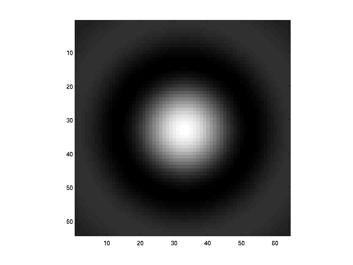
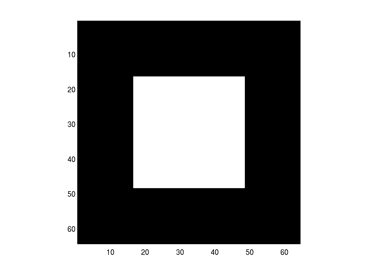
In this section, we show the convergence behavior of different iterative algorithms we discussed in section 3 by numerical experiments. In the cameraman image reconstruction experiment, we choose the illuminating probe a(𝐫)𝑎𝐫a({\bf r}) to be a 64×64646464\times 64 binary probe shown in Figure 4(a). The pixels within the 32×32323232\times 32 square at the center of the probe assume the value of 1. All other pixels take the value of 0. The zero padding of the inner 32×32323232\times 32 square ensures that the diffraction pattern of a 64×64646464\times 64 frame associated with this probe is oversampled in the reciprocal space. In the gold ball image reconstruction experiment, the illuminating probe is chosen to be the amplitude of the Fourier transform of an annular ring with inner radius of r15.4subscript𝑟15.4r_{1}\approx 5.4 and outer radius of r219.4subscript𝑟219.4r_{2}\approx 19.4. This probe mimics the true illumination used in a physical experiment.
Refer to caption
(a) The binary probe used in the reconstruction of the cameraman image.
Refer to caption
(b) The probe used in the reconstruction of the gold ball image.
Figure 4: The illuminating probes a(𝐫)𝑎𝐫a({\bf r}) used in ptychographic reconstructions of the cameraman and gold ball images.

In the cameraman experiment, the probe is translated by 888 pixels at a time in either horizontal or vertical direction. To prepare a stack of k𝑘k diffraction images bisubscript𝑏𝑖b_{i}, i=1,2,,k𝑖12𝑘i=1,2,...,k, we start from the upper left corner of the true image, extract a 64×64646464\times 64 frame, and multiply it with the probe, and then apply a 2D FFT to the product. The magnitude of transform is recorded and saved before we move either horizontally or vertically to obtain the next frame. If the lower right corner of the frame goes outside of the image (which does not happen in this particular case), we simply “wrap the probe around” the image as if the image is periodically extended. As a result, the total number of diffraction frames we use for each reconstruction is

k=25682568=1024.𝑘256825681024k=\frac{256}{8}\cdot\frac{256}{8}=1024.

As we will show in section 6.4, the size of translation, which determines the amount of overlap between adjacent frames, has a noticeable effect on the convergence of the iterative reconstruction algorithms.

Figure 5 shows the convergence history of several iterative algorithms discussed in section 3 when they are applied to the diffraction frames extracted from the cameraman image. We plot both the relative residual norm defined by

res=i=1k|zi|()bi2i=1kbi2,𝑟𝑒𝑠superscriptsubscript𝑖1𝑘superscriptnormsuperscriptsubscript𝑧𝑖subscript𝑏𝑖2superscriptsubscript𝑖1𝑘superscriptnormsubscript𝑏𝑖2res=\frac{\sqrt{\sum_{i=1}^{k}\||z_{i}|^{(\ell)}-b_{i}\|^{2}}}{\sqrt{\sum_{i=1}^{k}\|b_{i}\|^{2}}}, (63)

where |zi|()=|FQiψ()|superscriptsubscript𝑧𝑖𝐹subscript𝑄𝑖superscript𝜓|z_{i}|^{(\ell)}=|FQ_{i}\psi^{(\ell)}| and \ell is the iteration number, and the relative error of the reconstructed image defined by
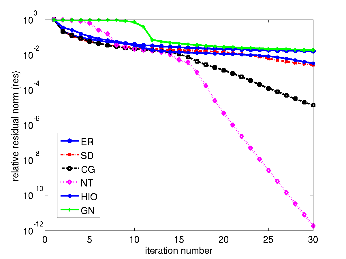
err=ψ()ψ^ψ^.𝑒𝑟𝑟normsuperscript𝜓^𝜓norm^𝜓err=\frac{\|\psi^{(\ell)}-\hat{\psi}\|}{\|\hat{\psi}\|}.
Refer to caption
(a) Change of the relative residual norm (res) for the reconstruction of the cameraman image.
Refer to caption
(b) Change of the relative error (err) for the reconstruction of the cameraman image.
Figure 5: A comparison of the convergence behavior of different iterative ptychographic reconstruction algorithms for the cameraman image.

In these runs, an exact line search is used in the steepest descent (SD), nonlinear conjugate gradient (CG). The Steihaug’s trust region technique implemented in [20] is used in the Newton’s method (NT). We set the starting guess of the solution ψ^^𝜓\hat{\psi} to

ψ(0)=(i=1kQiQi)1i=1kQibi.superscript𝜓0superscriptsuperscriptsubscript𝑖1𝑘superscriptsubscript𝑄𝑖subscript𝑄𝑖1superscriptsubscript𝑖1𝑘superscriptsubscript𝑄𝑖subscript𝑏𝑖\psi^{(0)}=\left(\sum_{i=1}^{k}Q_{i}^{\ast}Q_{i}\right)^{-1}\sum_{i=1}^{k}Q_{i}^{\ast}b_{i}.

It is clear from Figure 5 that NT converges much faster than the other algorithms. Its performance is followed by the CG algorithm which is much faster than the error reduction (ER), SD, Gauss-Newton (GN) and the hybrid input-output (HIO) algorithms. Similar convergence behavior is observed when other random starting guesses are used, although occasionally, a random starting guess can lead to stagnation or convergence to a local minimizer. We will discuss this issue in section 6.3. We set the maximum number of iterations allowed in all runs to 30. This is somewhat excessive for both NT and CG algorithms. Typically, when the relative error of the reconstructed image falls below 103superscript10310^{-3}, it is nearly impossible to visually distinguish the reconstruction from the true image. When the relative error is larger, the reconstructed cameraman images may contain visible artifacts such as those shown in Figures 6(a) and 6(b) which are produced at the end of the 30th ER and SD iterations respectively.

Refer to caption
(a) ER reconstruction
Refer to caption
(b) SD reconstruction
Figure 6: The reconstructed cameraman images by ER and SD algorithms contain visible ringing artifacts.

It is somewhat surprising that GN performs poorly on this problem. We believe the problem is that we used the MATLAB implementation of the large-scale Gauss-Newton algorithm, i.e., the function lsqnonlin in the MATLAB’s Optimization Toolbox, which does not handle functions of complex variable very well. Moreover, it is not easy to obtain the relative error associated with the approximate reconstruction produced at each iteration from this function.

For the reconstruction of the gold ball image, we choose the starting guess to be

ψ(0)=(i=1kQiQi)1i=1kQiDiag(bi)Diag(|ui|)1ui,superscript𝜓0superscriptsuperscriptsubscript𝑖1𝑘superscriptsubscript𝑄𝑖subscript𝑄𝑖1superscriptsubscript𝑖1𝑘superscriptsubscript𝑄𝑖Diagsubscript𝑏𝑖Diagsuperscriptsubscript𝑢𝑖1subscript𝑢𝑖\psi^{(0)}=\left(\sum_{i=1}^{k}Q_{i}^{\ast}Q_{i}\right)^{-1}\sum_{i=1}^{k}Q_{i}^{\ast}\mbox{Diag}\left(b_{i}\right)\mbox{Diag}\left(|u_{i}|\right)^{-1}u_{i},

where uisubscript𝑢𝑖u_{i} is a complex random vector, and the real and imaginary part of each component has a uniform distribution within [1,1]11[-1,1].

In this experiment, the probe is translated by a larger amount (16 pixels) in either horizontal or vertical direction. Figure 7 shows the convergence history of ER, SD, CG, HIO, and NT. From Figure 7(a), it appears that CG is the best among all the methods we tried. The HIO algorithm performs well in the first 60 iterations, but then stagnates. As we can see from Figure 7 that the neither the residual norm nor the relative error associated with HIO changes monotonically. This is not completely surprising because HIO does not try to minimize either objective functions. For this example, the performance of NT lags behind CG by a large margin although both algorithms exhibit monotonic convergence with a more predictable error reduction. We should mention that to measure the relative error associated with a reconstructed gold ball image ψ()superscript𝜓\psi^{(\ell)}, we need to multiply it by a constant phase factor γ𝛾\gamma first, i.e., the relative error is defined as
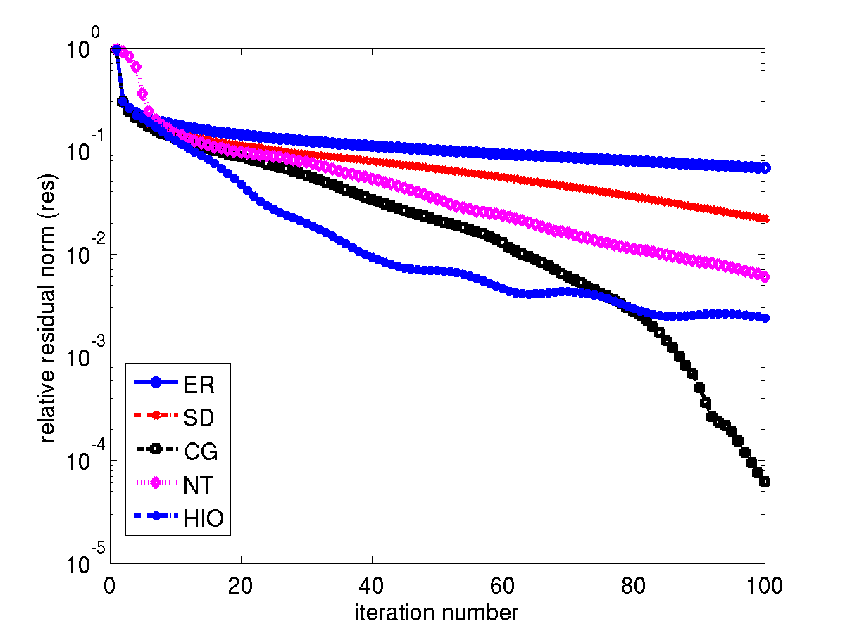
err=γψ()ψ^ψ^.𝑒𝑟𝑟norm𝛾superscript𝜓^𝜓norm^𝜓err=\frac{\|\gamma\psi^{(\ell)}-\hat{\psi}\|}{\|\hat{\psi}\|}.
Refer to caption
(a) Change of the relative residual norm (res) for the reconstruction of the gold ball image.
Refer to caption
(b) Change of the relative error (err) for the reconstruction of the gold ball image.
Figure 7: A comparison of the convergence behavior of different iterative ptychographic reconstruction algorithms for the gold ball image.

In Figure 8, we can clearly see that the magnitude of the reconstructed images produced by CG (Figure 8(a)) and HIO (Figure 8(c)) are nearly indistinguishable from the magnitude of the true image. However, the phase angles of the reconstructed image produced by CG (Figure 8(d)) appear to be better than those produced by HIO, which is indicated by the magnitude of the absolute errors |γψ()ψ^|𝛾superscript𝜓^𝜓|\gamma\psi^{(\ell)}-\hat{\psi}| shown in Figures 8(b) and 8(d).

Refer to caption
(a) The magnitude of the reconstructed gold ball image produced by the CG algorithm.
Refer to caption
(b) The magnitude of the error associated with the reconstructed gold ball image produced by the CG algorithm.
Refer to caption
(c) The magnitude of the reconstructed gold ball image produced by the HIO algorithm.
Refer to caption
(d) The magnitude of the error associated with the reconstructed gold ball image produced by the HIO algorithm.
Figure 8: The reconstructed cameraman images produced by CG and HIO.

6.2 The Effect of Preconditioning

As we indicated in Section 3.2, the use of a preconditioner can enhance the convergence of SD and CG. A natural preconditioner that is easy to construct is (43). However, this preconditioner is only effective, when the condition number of K𝐾K is relatively large. For the binary probe used in the reconstruction of the cameraman image, K=4I𝐾4𝐼K=4I. The condition number of this matrix is 1. Hence, using this preconditioner has no effect on the convergence of the CG iteration, as we can clearly see in Figure 9(a). The condition number associated with the probe used in the gold ball image reconstruction is around 4.5. Hence the effect of the preconditioner is negligible as we can see from Figure 9(b).
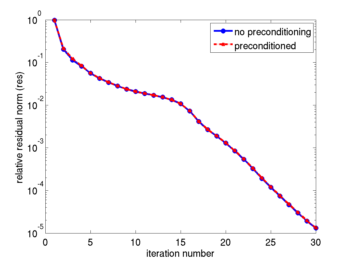
Refer to caption
(a) The effect of the preconditioner on the convergence of SD.
Refer to caption
(b) The effect of the preconditioner on the convergence of CG.
Figure 9: The effect of a preconditioner on the convergence of the CG algorithms applied to cameraman and gold ball image reconstruction.

6.3 Local Minimizer and the Choice of the Objective Function

As we indicated in section 2.2, based on the analytic Hessian and curvature expression, that neither ϵ(ψ)italic-ϵ𝜓\epsilon(\psi) nor ρ(ψ)𝜌𝜓\rho(\psi) is globally convex. This observation suggests that all iterative optimization algorithm discussed above may converge to a local minimizer. Although we found that in practice, local minimizers are not easy to find, they do exist as the following example show.

In order to find a local minimizer, we construct many random starting guesses using the MATLAB rand function. To save time, we chose to reconstruct a 64×64646464\times 64 subimage of the cameraman image shown in Figure 2. This subimage is shown in Figure 12(a). A 16×16161616\times 16 binary probe that has a value 1 in the 8×8888\times 8 center of the probe and 0 elsewhere is used. The diffraction stack consisting of 646464 diffraction images is obtained by translating the probe 4 pixels a time in either the horizontal and vertical direction.

Figure 10 shows that one of the random starting guesses lead to the convergence of the CG algorithm to a local minimizer. In particular, the relative residual (63) which is proportional to the objective function ρ𝜌\rho stagnates around 0.9 after the first 15 iterations (Figure 10(a)), whereas the relative gradient ρ(ψ())/ψ^norm𝜌superscript𝜓norm^𝜓\|\nabla\rho(\psi^{(\ell)})\|/\|\hat{\psi}\| decreases to 108superscript10810^{-8} after 40 iterations.

Figure 12(b) shows how the reconstructed image compares with the true image for this particular starting guess used. In this case, the local minimizer appears to contain visible artifacts in a small region near top of the tripod. The amplitude of this localized error is also revealed in the relative error plot shown in Figure 11(a). The phase error associated with a particular frame of the reconstruction obtained from

Qiψ¯|Qiψ|Qiψ^|Qiψ^|,¯subscript𝑄𝑖𝜓subscript𝑄𝑖𝜓subscript𝑄𝑖^𝜓subscript𝑄𝑖^𝜓\frac{\overline{Q_{i}\psi}}{|Q_{i}\psi|}\cdot\frac{Q_{i}\hat{\psi}}{|Q_{i}\hat{\psi}|},

for some particular Qisubscript𝑄𝑖Q_{i} is shown in Figure 11(b).

Refer to caption
(a) Change of the relative residual norm (res).
Refer to caption
(b) Change of the relative gradient.
Figure 10: The convergence of CG to a local minimizer.
Refer to caption
(a) Amplitude error in the reconstruct image
Refer to caption
(b) Phase error in degrees associated with a particular frame
Figure 11: The error associated with a local minimizer.
Refer to caption
(a) True image.
Refer to caption
(b) The reconstructed image (a local minimizer).
Figure 12: The artifacts produced by a local minimizer of ρ𝜌\rho.

We should also note that for this particular starting guess, all methods we tried converged to the same local minmizer. This is not all that surprising. It simply shows (empirically) that local minimizers of (2) exists, and our starting guess is sufficiently close to it.

However, what is interesting is that if we choose to minimize  (3) by using any one of the iterative methods discussed above from the same starting guess, we are able to obtain the correct solution. For examples, Figure 13(a) shows that when the NT applied to the weighted (scaled) objective function

ϵ~(ψ)=12i=1k(|zi|2bi2)TDiag(bi)1(|zi|2bi2),\tilde{\epsilon}_{(}\psi)=\frac{1}{2}\sum_{i=1}^{k}(|z_{i}|^{2}-b_{i}^{2})^{T}\mbox{Diag}\left(b_{i}\right)^{-1}(|z_{i}|^{2}-b_{i}^{2}), (64)

where |zi|=|FQiψ|subscript𝑧𝑖𝐹subscript𝑄𝑖𝜓|z_{i}|=|FQ_{i}\psi| and bi=|FQiψ^|subscript𝑏𝑖𝐹subscript𝑄𝑖^𝜓b_{i}=|FQ_{i}\hat{\psi}|, an accurate reconstruction can be obtained in roughly 350 iterations. Admittedly, the convergence rate is much slower in this case when compared to the convergence of NT when it’s applied to (2) from a different starting point. The convergence is even slower if no weighting (or scaling) is used, i.e. when (3) is used as the objective function. However, the fact that convergence can be reached for (64) but not (2) from the same starting point is quite interesting. Furthermore, Figure 13(b) shows that if we take the local minimizer returned from an iterative minimization of (2) as the starting guess for minimizing (64), convergence can be reached in 12 iterations. This experiment suggests that it may be useful to have a hybrid optimization scheme in which (2) is minimized first. If a local minimizer of (2) is identified, one can then try to minimize (64) starting from the local minimizer of (2).
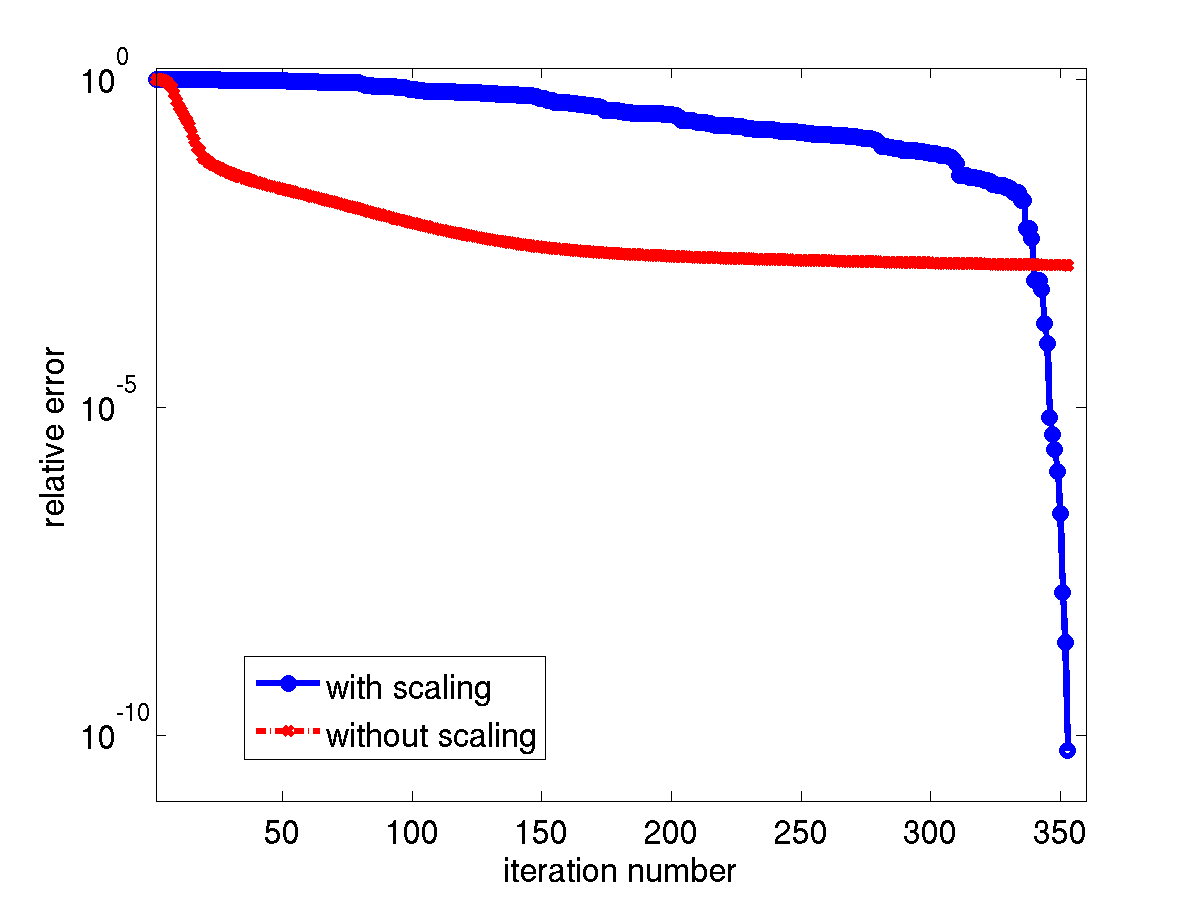
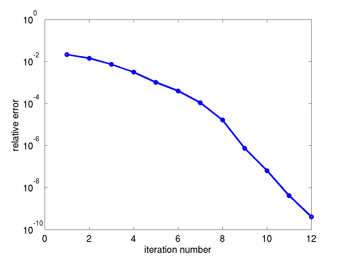
Refer to caption
(a) The convergence of the NT algorithm when it is applied to (3) (red) and (64). The starting guess chosen in these runs is the same one used in the minimization of (2).
Refer to caption
(b) The convergence of the NT algorithm when the starting guess is chosen to be the local minimizer shown in Figure 12(b)
Figure 13: The convergence of the NT algorithm when applied to (3) (red) and (64) (blue).

6.4 The Effect of Overlapping on the Convergence of Iterative Algorithm

As we alluded to earlier, the amount of overlap between two adjacent diffraction frames has a noticeable effect on the convergence of optimization based iteration algorithms (e.g., CG, NT, SD etc.) used to reconstruct the true image. Although we currently do not have a clear way to quantify such an effect mathematically, the following examples demonstrate this effect.

In the first example, we try to reconstruct the gold ball image from four different diffraction stacks. Each stack contains a set of 64×64646464\times 64 diffraction frames. These frames are generated by translating the probe shown in Figure 4(b) by different amount in horizontal and vertical directions. The larger the translation, the smaller the overlap is between two adjacent images. Figure 15(a) shows that CG converges very slowly when the diffraction stack contains diffraction frames obtained by translating the probe 202020 pixels at a time (the black curve). Faster convergence is observed when the amount of translation is decreased to Δx=16,12,8Δ𝑥16128\Delta x=16,12,8. It is interesting to see from Figure 15(b) that the amount of overlap does not affect the convergence of the HIO algorithm.

In the second example, we try to reconstruct the gold ball image from 1024 diffraction frames of 128×128128128128\times 128 pixels. The illumination function is similar to that used in Figure 4. It is scaled by a factor of 2 to 128×128128128128\times 128 pixels. The probe FWHM (full width at half maximum) is 30 pixels. We choose to fix the number of frames. So the reconstructed area increases with step size. When probe is near the edge of the image, we “wrap it around the edge” as if the image itself is periodically extended. The overlap is varied by changing the step size ΔxΔ𝑥\Delta x. The larger the ΔxΔ𝑥\Delta x, the smaller the amount of overlap.

The starting point is produced from a random number generator for each test. A range of step sizes between 6 and 30 pixels have been tried. For a fixed step size, the test is repeated 100 times. We observe that the step size ΔxΔ𝑥\Delta x does not influence the convergence rate up to Δx20similar-to-or-equalsΔ𝑥20\Delta x\simeq 20. Figures 14(a) and  14(c) show that the conjugate gradient method converges in less than 400 iterations, while the RAAR algorithm requires almost 1500 iterations. Figures 14(b) and 14(d) illustrate the percentage of successful runs started from a random guess for each of the step sizes 0Δx300Δ𝑥300\leq\Delta x\leq 30. The percentage of successful runs (shown in color) is plotted against the maximum number of allowed iterations. When Δx20Δ𝑥20\Delta x\leq 20, both CG and RAAR converge nearly 100% of the time when a relatively small number of iterations are used in these methods. However, when 20Δx2520Δ𝑥2520\leq\Delta x\leq 25, more iterations are required to ensure the convergence of CG and RAAR. When 25Δx3025Δ𝑥3025\leq\Delta x\leq 30, CG appears to stagnate for all random starting guesses we tried, whereas RAAR can still converge when a very large number of iterations are taken.
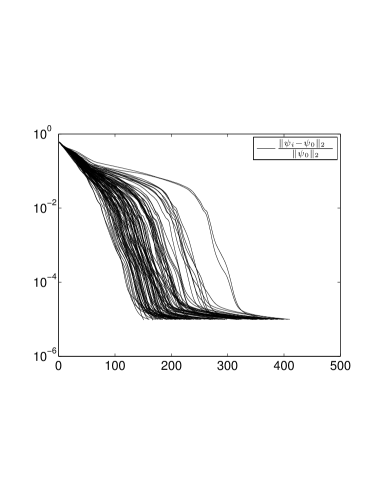
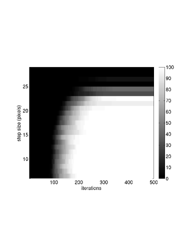
Refer to caption
(a) convergence of CG from 100 random starts Δx=20Δ𝑥20\Delta x=20
Refer to caption
(b) percentage tests that converge to err104𝑒𝑟𝑟superscript104err\leq 10^{-4}
Refer to caption
(c) convergence of RAAR from 100 random starts Δx=20Δ𝑥20\Delta x=20
Refer to caption
(d) percentage of RAAR iterations that converge to an error of 104superscript10410^{-4}
Figure 14: The convergence rate of the CG and RAAR methods from different random starting points.

To explain the effect of overlapping on the convergence of optimization based iterative algorithms such as the nonlinear CG, we examine the structure of the Hessian of the objective function ρ𝜌\rho in (2). It follows from (25)-(26) that the Hρsuperscript𝐻𝜌H^{\rho} can be written as

Hρ=((F^Q)(F^Q)T)(B11B12B21B22)(F^QF^¯Q¯),superscript𝐻𝜌superscript^𝐹𝑄superscript^𝐹𝑄𝑇subscript𝐵11subscript𝐵12subscript𝐵21subscript𝐵22^𝐹𝑄¯^𝐹¯𝑄H^{\rho}=\left((\hat{F}Q)^{\ast}\ \ (\hat{F}Q)^{T}\right)\left(\begin{array}[]{cc}B_{11}&B_{12}\\ B_{21}&B_{22}\end{array}\right)\left(\begin{array}[]{c}\hat{F}Q\\ \bar{\hat{F}}\bar{Q}\end{array}\right), (65)

where B11=B22¯subscript𝐵11¯subscript𝐵22B_{11}=\overline{{B}_{22}} and B12=B21subscript𝐵12superscriptsubscript𝐵21B_{12}=B_{21}^{\ast} are all diagonal, F^^𝐹\hat{F} is a block diagonal matrix of discrete Fourier transforms, i.e. F^=Diag(F,F,,F)^𝐹Diag𝐹𝐹𝐹\hat{F}=\mbox{Diag}\left(F,F,...,F\right), and Q=(Q1Q2Qk)𝑄superscriptsuperscriptsubscript𝑄1superscriptsubscript𝑄2superscriptsubscript𝑄𝑘Q=(Q_{1}^{\ast}\>Q_{2}^{\ast}\>...\>Q_{k}^{\ast})^{\ast}. The diagonal elements of B11subscript𝐵11B_{11} and B12subscript𝐵12B_{12} are simply 1βji/(2ζji)1subscript𝛽𝑗𝑖2subscript𝜁𝑗𝑖1-\beta_{ji}/(2\zeta_{ji}) and βjiζji2/(2|ζji|3)subscript𝛽𝑗𝑖superscriptsubscript𝜁𝑗𝑖22superscriptsubscript𝜁𝑗𝑖3\beta_{ji}\zeta_{ji}^{2}/(2|\zeta_{ji}|^{3}) respectively for i=1,2,,k𝑖12𝑘i=1,2,...,k and j=1,2,,m𝑗12𝑚j=1,2,...,m.

We will show that Hρsuperscript𝐻𝜌H^{\rho} is diagonal dominant when there is a sufficient amount of overlap between adjacent diffraction frames. To simplify our discussion, let us assume for the moment that bisubscript𝑏𝑖b_{i} is a 1D diffraction pattern obtained from a binary probe that illuminates three pixels at a time, and the probe is translated one pixel at a time so that the image frame that produces bisubscript𝑏𝑖b_{i} overlaps with that produces bi1subscript𝑏𝑖1b_{i-1} by two pixels. In this case, the F^Q^𝐹𝑄\hat{F}Q term in (65) has the form

(f1f2f300f2f300f3fkf100fkf1f20fk),subscript𝑓1subscript𝑓2subscript𝑓300subscript𝑓2subscript𝑓300subscript𝑓3subscript𝑓𝑘subscript𝑓100subscript𝑓𝑘subscript𝑓1subscript𝑓20subscript𝑓𝑘\left(\begin{array}[]{ccccc}f_{1}&f_{2}&f_{3}&\ldots&0\\ 0&f_{2}&f_{3}&\ddots&\vdots\\ 0&0&f_{3}&\ddots&f_{k}\\ f_{1}&0&0&\ddots&f_{k}\\ f_{1}&f_{2}&0&\ldots&f_{k}\end{array}\right),

where fisubscript𝑓𝑖f_{i} is the i𝑖ith column of F𝐹F.

As a result, a typical diagonal term of Hρsuperscript𝐻𝜌H^{\rho} has the form

Hi,iρ=fiDi2fi+fiDi1fi+fiDifi=trace(Di2+Di1+Di),subscriptsuperscript𝐻𝜌𝑖𝑖superscriptsubscript𝑓𝑖subscript𝐷𝑖2subscript𝑓𝑖superscriptsubscript𝑓𝑖subscript𝐷𝑖1subscript𝑓𝑖superscriptsubscript𝑓𝑖subscript𝐷𝑖subscript𝑓𝑖tracesubscript𝐷𝑖2subscript𝐷𝑖1subscript𝐷𝑖H^{\rho}_{i,i}=f_{i}^{\ast}D_{i-2}f_{i}+f_{i}^{\ast}D_{i-1}f_{i}+f_{i}^{\ast}D_{i}f_{i}=\mbox{trace}(D_{i-2}+D_{i-1}+D_{i}), (66)

where Disubscript𝐷𝑖D_{i} is a diagonal matrix that contains elements 1βji/(2ζji)1subscript𝛽𝑗𝑖2subscript𝜁𝑗𝑖1-\beta_{ji}/(2\zeta_{ji}) for j=1,2,3𝑗123j=1,2,3.

When ψ𝜓\psi is near the solution, zisubscript𝑧𝑖z_{i} is close to bisubscript𝑏𝑖b_{i}. Hence, Disubscript𝐷𝑖D_{i} is likely to contain positive entries only. Therefore, the diagonal elements of Hρsuperscript𝐻𝜌H^{\rho} are likely to be much larger compared to the nonzero off-diagonal elements which contain terms in the form of either fjDifsuperscriptsubscript𝑓𝑗subscript𝐷𝑖subscript𝑓f_{j}^{\ast}D_{i}f_{\ell} and its conjugate, where j𝑗j\neq\ell, or fjTEifsuperscriptsubscript𝑓𝑗𝑇subscript𝐸𝑖subscript𝑓f_{j}^{T}E_{i}f_{\ell} and its conjugate, where Eisubscript𝐸𝑖E_{i} is a diagonal matrix (and part of B12subscript𝐵12B_{12}) that contains elements βjiζji2/(2|ζji|3)subscript𝛽𝑗𝑖superscriptsubscript𝜁𝑗𝑖22superscriptsubscript𝜁𝑗𝑖3\beta_{ji}\zeta_{ji}^{2}/(2|\zeta_{ji}|^{3}) for j=1,2,3𝑗123j=1,2,3. Due to the phase difference between fjsubscript𝑓𝑗f_{j} and fsubscript𝑓f_{\ell}, Disubscript𝐷𝑖D_{i}’s do not add up “coherently” on the off-diagonal of Hρsuperscript𝐻𝜌H^{\rho} as they do on the diagonal. Neither do nonzero entries in Eisubscript𝐸𝑖E_{i}’s add up coherently on the off-diagonal blocks of Hρsuperscript𝐻𝜌H^{\rho} either. Hence, the matrix Hρsuperscript𝐻𝜌H^{\rho} becomes diagonal dominant when there is larger amount of overlap between two adjacent frames. In fact, the diagonal of Hρsuperscript𝐻𝜌H^{\rho} may become so dominant that the spectral property of Hρsuperscript𝐻𝜌H^{\rho} is determined largely by the diagonal part of the matrix, which is typically well conditioned due to the averaging of Disubscript𝐷𝑖D_{i} in (66). This observation provides an intuitive explaination on why increasing the amount of overlap between adjacent frames tends to improve the convergence rate of CG and other optimization based iterative ptychographical phase retrieval algorithms. Although this is not a precise analysis of the spectral property of Hρsuperscript𝐻𝜌H^{\rho}, the analysis does match with observations made in our numerical expriments. Moreover, this type of analysis can be extended to the 2D case in which F𝐹F is represented as a tensor product of two 1D discrete Fourier transforms.
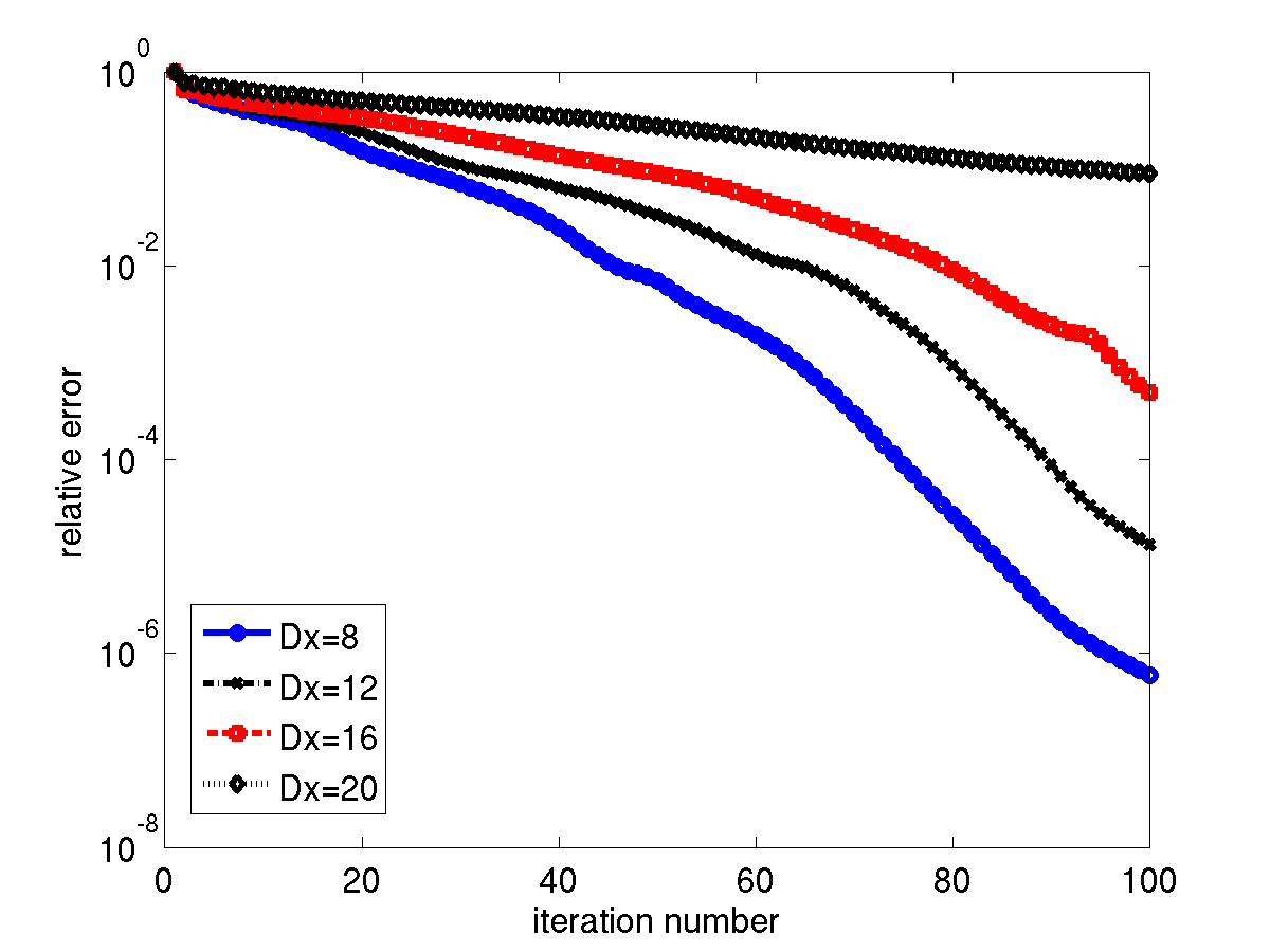
Refer to caption
(a) The effect of overlapping on the convergence of CG for the gold ball image reconstruction.
Refer to caption
(b) The effect of overlapping on the convergence of HIO for the gold ball image reconstruction.
Figure 15: The effect of overlapping on the convergence of CG and HIO algorithms.

7 Conclusion

We formulated the ptychographic phase retrieval problem as a nonlinear optimization problem and discussed how standard iterative optimization algorithms can be applied to solve this problem.

We showed that the optimization problems we solve are not globally convex. Hence standard optimization algorithms can produce local minimizers. However, the Hessian of the objective functions we minimize do have special structures that may be exploited.

We compared the performance of several optimization algorithms and found that Newton’s method with Steihaug’s trust region technique gave the best performance on a real valued image. For a complex valued image, the nonlinear conjugate gradient algorithm appears to perform better.

We discussed the effect of preconditioning on convergence of the CG algorithm. We also demonstrated it is possible for an optimization algorithm to converge to a local minimizer although in practice such type of convergence failure is rare, especially when the amount of overlap between two adjacent diffraction frames is large.

We demonstrated by a numerical example that the convergence rate of an optimization algorithm depends on the amount of overlapping between two adjacent diffraction frames. We provided an intuitive analysis on why this occurs. More research is needed to provide a more precise analysis on this phenonmenon.

We identified the connection between the optimization based approach with both Wigner deconvolution and projection algorithms often used in phase retrieval literatures. We pointed out the limitation of Wigner deconvolution and showed that the optimization based algorithm tend to perform better than projection algorithms such as HIO when the amount of overlap between adjacent images is sufficiently large.

Acknowledgment

This work was supported by the Laboratory Directed Research and Development Program of Lawrence Berkeley National Laboratory under the U.S. Department of Energy contract number DE-AC02-05CH11231 (C. Y., A. S., S. M.), the National Science Foundation Grant 0810104 (J. Q.) and by the Director, Office of Science, Advanced Scientific Computing Research, of the U.S. Department of Energy under Contract No. DE-AC02-05CH11231 (F.M.). The computational results presented were obtained at the National Energy Research Scientific Computing Center (NERSC), which is supported by the Director, Office of Advanced Scientific Computing Research of the U.S. Department of Energy under contract number DE-AC02-05CH11232.