Parallel Coordinate Descent for -Regularized Loss Minimization
Abstract
We propose Shotgun, a parallel coordinate descent algorithm for minimizing -regularized losses. Though coordinate descent seems inherently sequential, we prove convergence bounds for Shotgun which predict linear speedups, up to a problem-dependent limit. We present a comprehensive empirical study of Shotgun for Lasso and sparse logistic regression. Our theoretical predictions on the potential for parallelism closely match behavior on real data. Shotgun outperforms other published solvers on a range of large problems, proving to be one of the most scalable algorithms for .
1 Introduction
Many applications use -regularized models such as the Lasso (Tibshirani, 1996) and sparse logistic regression (Ng, 2004). regularization biases learning towards sparse solutions, and it is especially useful for high-dimensional problems with large numbers of features. For example, in logistic regression, it allows sample complexity to scale logarithmically w.r.t. the number of irrelevant features (Ng, 2004).
Much effort has been put into developing optimization algorithms for models. These algorithms range from coordinate minimization (Fu, 1998) and stochastic gradient (Shalev-Shwartz & Tewari, 2009) to more complex interior point methods (Kim et al., 2007).
Coordinate descent, which we call Shooting after Fu (1998), is a simple but very effective algorithm which updates one coordinate per iteration. It often requires no tuning of parameters, unlike, e.g., stochastic gradient. As we discuss in Sec. 2, theory (Shalev-Shwartz & Tewari, 2009) and extensive empirical results (Yuan et al., 2010) have shown that variants of Shooting are particularly competitive for high-dimensional data.
The need for scalable optimization is growing as more applications use high-dimensional data, but processor core speeds have stopped increasing in recent years. Instead, computers come with more cores, and the new challenge is utilizing them efficiently. Yet despite the many sequential optimization algorithms for -regularized losses, few parallel algorithms exist.
Some algorithms, such as interior point methods, can benefit from parallel matrix-vector operations. However, we found empirically that such algorithms were often outperformed by Shooting.
Recent work analyzes parallel stochastic gradient descent for multicore (Langford et al., 2009b) and distributed settings (Mann et al., 2009; Zinkevich et al., 2010). These methods parallelize over samples. In applications using regularization, though, there are often many more features than samples, so parallelizing over samples may be of limited utility. 000 These authors contributed equally to this work.
We therefore take an orthogonal approach and parallelize over features, with a remarkable result: we can parallelize coordinate descent—an algorithm which seems inherently sequential—for -regularized losses. In Sec. 3, we propose Shotgun, a simple multicore algorithm which makes coordinate updates in parallel. We prove strong convergence bounds for Shotgun which predict speedups over Shooting which are linear in , up to a problem-dependent maximum . Moreover, our theory provides an estimate for this ideal which may be easily computed from the data.
Parallel coordinate descent was also considered by Tsitsiklis et al. (1986), but for differentiable objectives in the asynchronous setting. They give a very general analysis, proving asymptotic convergence but not convergence rates. We are able to prove rates and theoretical speedups for our class of objectives.
In Sec. 4, we compare multicore Shotgun with five state-of-the-art algorithms on 35 real and synthetic datasets. The results show that in large problems Shotgun outperforms the other algorithms. Our experiments also validate the theoretical predictions by showing that Shotgun requires only about as many iterations as Shooting. We measure the parallel speedup in running time and analyze the limitations imposed by the multicore hardware.
2 -Regularized Loss Minimization
We consider optimization problems of the form
| (1) |
where is a non-negative convex loss. Each of samples has a feature vector and observation (where ). is an unknown vector of weights for features. is a regularization parameter. Let be the design matrix, whose row is . Assume w.l.o.g. that columns of are normalized s.t. .111Normalizing does not change the objective if a separate, normalized is used for each .
An instance of (1) is the Lasso (Tibshirani, 1996) (in penalty form), for which and
| (2) |
as well as sparse logistic regression (Ng, 2004), for which and
| (3) |
For analysis, we follow Shalev-Shwartz and Tewari (2009) and transform (1) into an equivalent problem with a twice-differentiable regularizer. We let , use duplicated features , and solve
| (4) |
If minimizes (4), then minimizes (1). Though our analysis uses duplicate features, they are not needed for an implementation.
2.1 Sequential Coordinate Descent
Shalev-Shwartz and Tewari (2009) analyze Stochastic Coordinate Descent (SCD), a stochastic version of Shooting for solving (1). SCD (Alg. 1) randomly chooses one weight to update per iteration. It computes the update via
| (5) |
where is a loss-dependent constant.
To our knowledge, Shalev-Shwartz and Tewari (2009) provide the best known convergence bounds for SCD. Their analysis requires a uniform upper bound on the change in the loss from updating a single weight:
Assumption 2.1.
Let be a convex function. Assume there exists s.t., for all and single-weight updates , we have:
where is a unit vector with in its entry. For the losses in (2) and (3), Taylor expansions give
| (6) |
Using this bound, they prove the following theorem.
Theorem 2.1.
As Shalev-Shwartz and Tewari (2009) argue, Theorem 2.1 indicates that SCD scales well in the dimensionality of the data. For example, it achieves better runtime bounds w.r.t. than stochastic gradient methods such as SMIDAS (Shalev-Shwartz & Tewari, 2009) and truncated gradient (Langford et al., 2009a).
3 Parallel Coordinate Descent
As the dimensionality or sample size increase, even fast sequential algorithms become expensive. To scale to larger problems, we turn to parallel computation. In this section, we present our main theoretical contribution: we show coordinate descent can be parallelized by proving strong convergence bounds.
We parallelize stochastic Shooting and call our algorithm Shotgun (Alg. 2). Shotgun initially chooses , the number of weights to update in parallel. On each iteration, it chooses weights independently and uniformly at random from ; these form a multiset . It updates each in parallel using the same update as Shooting (5). Let be the collective update to , i.e., .
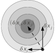
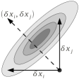
Intuitively, parallel updates might increase the risk of divergence. In Fig. 1, in the left subplot, parallel updates speed up convergence since features are uncorrelated; in the right subplot, parallel updates of correlated features risk increasing the objective. We can avoid divergence by imposing a step size, but our experiments showed that approach to be impractical.222A step size of ensures convergence since is convex in , but it results in very small steps and long runtimes.
We formalize this intuition for the Lasso in Theorem 3.1. We can separate a sequential progress term (summing the improvement from separate updates) from a term measuring interference between parallel updates. If were normalized and centered to be a covariance matrix, the elements in the interference term’s sum would be non-zero only for correlated variables, matching our intuition from Fig. 1. Harmful interference could occur when, e.g., and features were positively correlated.
Theorem 3.1.
Fix . If is the collective update to in one iteration of Alg. 2 for the Lasso, then
Proof Sketch333We include detailed proofs of all theorems and lemmas in the supplementary material.:
Write the Taylor expansion of around .
Bound the first-order term using (5).
In the next section, we show that this intuition holds for the more general
optimization problem in (1).
 |
 |
3.1 Shotgun Convergence Analysis
In this section, we present our convergence result for Shotgun. The result provides a problem-specific measure of the potential for parallelization: the spectral radius of (i.e., the maximum of the magnitudes of eigenvalues of ). Moreover, this measure is prescriptive: may be estimated via, e.g., power iteration444For our datasets, power iteration gave reasonable estimates within a small fraction of the total runtime. (Strang, 1988), and it provides a plug-in estimate of the ideal number of parallel updates.
We begin by generalizing Assumption 2.1 to our parallel setting. The scalars for Lasso and logistic regression remain the same as in (6).
Assumption 3.1.
Let be a convex function. Assume that there exists such that, for all and parallel updates , we have
We now state our main result, generalizing the convergence bound in Theorem 2.1 to the Shotgun algorithm.
Theorem 3.2.
Without duplicated features, Theorem 3.2 predicts that we can do up to parallel updates and achieve speedups linear in . We denote the predicted maximum as . For an ideal problem with uncorrelated features, , so we could do up to parallel updates. For a pathological problem with exactly correlated features, , so our theorem tells us that we could not do parallel updates. With , we recover the result for Shooting in Theorem 2.1.
To prove Theorem 3.2, we first bound the negative impact of interference between parallel updates.
Lemma 3.3.
Proof Sketch: Take the expectation w.r.t. of the inequality in Assumption 3.1.
| (8) |
Separate the diagonal elements from the second order term, and rewrite the expectation using our independent choices of . (Here, is the update given by (5), regardless of whether .)
| (9) |
Upper bound the double expectation in terms of by expressing the spectral radius of as .
| (10) |
Combine (10) back into (9), and rearrange terms to get the lemma’s result.
Proof Sketch (Theorem 3.2): Our proof resembles Shalev-Shwartz and Tewari (2009)’s proof of Theorem 2.1. The result from Lemma 3.3 replaces Assumption 2.1. One bound requires .
Our analysis implicitly assumes that parallel updates of the same weight will not make negative. Proper write-conflict resolution can ensure this assumption holds and is viable in our multicore setting.
3.2 Theory vs. Empirical Performance
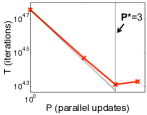
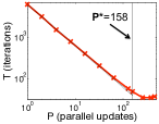
We end this section by comparing the predictions of Theorem 3.2 about the number of parallel updates with empirical performance for Lasso. We exactly simulated Shotgun as in Alg. 2 to eliminate effects from the practical implementation choices made in Sec. 4. We tested two single-pixel camera datasets from Duarte et al. (2008) with very different , estimating by averaging 10 runs of Shotgun. We used for Ball64_singlepixcam to get with about non-zeros; we used for Mug32_singlepixcam to get about non-zeros.
Fig. 2 plots versus the iterations required for to come within of the optimum . Theorem 3.2 predicts that should decrease as as long as . The empirical behavior follows this theory: using the predicted gives almost optimal speedups, and speedups are almost linear in . As exceeds , Shotgun soon diverges.
 |
 |
| Data: Ball64_singlepixcam | Data: Mug32_singlepixcam |
| , | , |
Thick red lines trace for increasing (until too large caused divergence). Vertical lines mark . Dotted diagonal lines show optimal (linear) speedups (partly hidden by solid line in right-hand plot).
Fig. 2 confirms Theorem 3.2’s result: Shooting, a seemingly sequential algorithm, can be parallelized and achieve near-linear speedups, and the spectral radius of succinctly captures the potential for parallelism in a problem. To our knowledge, our convergence results are the first for parallel coordinate descent for -regularized losses, and they apply to any convex loss satisfying Assumption 3.1. Though Fig. 2 ignores certain implementation issues, we show in the next section that Shotgun performs well in practice.
3.3 Beyond
Theorems 2.1 and 3.2 generalize beyond , for their main requirements (Assumptions 2.1, 3.1) apply to a more general class of problems: s.t. , where is smooth. We discuss Shooting and Shotgun for sparse regression since both the method (coordinate descent) and problem (sparse regression) are arguably most useful for high-dimensional settings.
4 Experimental Results
We present an extensive study of Shotgun for the Lasso and sparse logistic regression. On a wide variety of datasets, we compare Shotgun with published state-of-the-art solvers. We also analyze self-speedup in detail in terms of Theorem 3.2 and hardware issues.
4.1 Lasso
We tested Shooting and Shotgun for the Lasso against five published Lasso solvers on 35 datasets. We summarize the results here; details are in the supplement.
4.1.1 Implementation: Shotgun
Our implementation made several practical improvements to the basic Shooting and Shotgun algorithms.
Following Friedman et al. (2010), we maintained a vector to avoid repeated computation. We also used their pathwise optimization scheme: rather than directly solving with the given , we solved with an exponentially decreasing sequence . The solution for is used to warm-start optimization for . This scheme can give significant speedups.
Though our analysis is for the synchronous setting, our implementation was asynchronous because of the high cost of synchronization. We used atomic compare-and-swap operations for updating the vector.
We used C++ and the CILK++ library (Leiserson, 2009) for parallelism. All tests ran on an AMD processor using up to eight Opteron 8384 cores (2.69 GHz).
4.1.2 Other Algorithms
L1_LS (Kim et al., 2007) is a log-barrier interior point method. It uses Preconditioned Conjugate Gradient (PCG) to solve Newton steps iteratively and avoid explicitly inverting the Hessian. The implementation is in Matlab, but the expensive step (PCG) uses very efficient native Matlab calls. In our tests, matrix-vector operations were parallelized on up to 8 cores.
FPC_AS (Wen et al., 2010) uses iterative shrinkage to estimate which elements of should be non-zero, as well as their signs. This reduces the objective to a smooth, quadratic function which is then minimized.
GPSR_BB (Figueiredo et al., 2008) is a gradient projection method which uses line search and termination techniques tailored for the Lasso.
Hard_l0 (Blumensath & Davies, 2009) uses iterative hard thresholding for compressed sensing. It sets all but the largest weights to zero on each iteration. We set as the sparsity obtained by Shooting.
SpaRSA (Wright et al., 2009) is an accelerated iterative shrinkage/thresholding algorithm which solves a sequence of quadratic approximations of the objective.
As with Shotgun, all of Shooting, FPC_AS, GPSR_BB, and SpaRSA use pathwise optimization schemes.
4.1.3 Results
 |
 |
 |
 |
| (a) Sparco | (b) Single-Pixel Camera | (c) Sparse Compressed Img. | (d) Large, Sparse Datasets |
| , avg 2987 | , avg 7688 | , avg 1143 | |
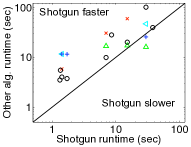
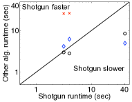
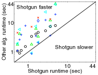
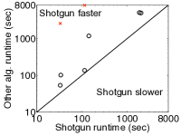
We divide our comparisons into four categories of datasets; the supplementary material has descriptions.
-
Sparco: Real-valued datasets of varying sparsity from the Sparco testbed (van den Berg et al., 2009).
, .
Single-Pixel Camera: Dense compressed sensing problems from Duarte et al. (2008).
, .
Sparse Compressed Imaging: Similar to Single-Pixel Camera datasets, but with very sparse random measurement matrices. Created by us.
, .
Large, Sparse Datasets: Very large and sparse problems, including predicting stock volatility from text in financial reports (Kogan et al., 2009).
, .
We ran each algorithm on each dataset with regularization and . Fig. 3 shows runtime results, divided by dataset category. We omit runs which failed to converge within a reasonable time period.
Shotgun (with ) consistently performs well, converging faster than other algorithms on most dataset categories. Shotgun does particularly well on the Large, Sparse Datasets category, for which most algorithms failed to converge anywhere near the ranges plotted in Fig. 3. The largest dataset, whose features are occurrences of bigrams in financial reports (Kogan et al., 2009), has 5 million features and 30K samples. On this dataset, Shooting converges but requires seconds, while Shotgun takes seconds.
On the Single-Pixel Camera datasets, Shotgun () is slower than Shooting. In fact, it is surprising that Shotgun converges at all with , for the plotted datasets all have . Fig. 2 shows Shotgun with diverging for the Ball64_singlepixcam dataset; however, after the practical adjustments to Shotgun used to produce Fig. 3, Shotgun converges with .
Among the other solvers, L1_LS is the most robust and even solves some of the Large, Sparse Datasets.
It is difficult to compare optimization algorithms and their implementations. Algorithms’ termination criteria differ; e.g., primal-dual methods such as L1_LS monitor the duality gap, while Shotgun monitors the change in . Shooting and Shotgun were written in C++, which is generally fast; the other algorithms were in Matlab, which handles loops slowly but linear algebra quickly. Therefore, we emphasize major trends: Shotgun robustly handles a range of problems; Theorem 3.2 helps explain its speedups; and Shotgun generally outperforms published solvers for the Lasso.
4.2 Sparse Logistic Regression
For logistic regression, we focus on comparing Shotgun with Stochastic Gradient Descent (SGD) variants. SGD methods are of particular interest to us since they are often considered to be very efficient, especially for learning with many samples; they often have convergence bounds independent of the number of samples.
For a large-scale comparison of various algorithms for sparse logistic regression, we refer the reader to the recent survey by Yuan et al. (2010). On L1_logreg (Koh et al., 2007) and CDN (Yuan et al., 2010), our results qualitatively matched their survey. Yuan et al. (2010) do not explore SGD empirically.
4.2.1 Implementation: Shotgun CDN
As Yuan et al. (2010) show empirically, their Coordinate Descent Newton (CDN) method is often orders of magnitude faster than the basic Shooting algorithm (Alg. 1) for sparse logistic regression. Like Shooting, CDN does coordinate descent, but instead of using a fixed step size, it uses a backtracking line search starting at a quadratic approximation of the objective.
Although our analysis uses the fixed step size in (5), we modified Shooting and Shotgun to use line searches as in CDN. We refer to CDN as Shooting CDN, and we refer to parallel CDN as Shotgun CDN.
Shooting CDN and Shotgun CDN maintain an active set of weights which are allowed to become non-zero; this scheme speeds up optimization, though it can limit parallelism by shrinking .
4.2.2 Other Algorithms
SGD iteratively updates in a gradient direction estimated with one sample and scaled by a learning rate. We implemented SGD in C++ following, e.g., Zinkevich et al. (2010). We used lazy shrinkage updates (Langford et al., 2009a) to make use of sparsity in . Choosing learning rates for SGD can be challenging. In our tests, constant rates led to faster convergence than decaying rates (decaying as ). For each test, we tried 14 exponentially increasing rates in (in parallel) and chose the rate giving the best training objective. We did not use a sparsifying step for SGD.
SMIDAS (Shalev-Shwartz & Tewari, 2009) uses stochastic mirror descent but truncates gradients to sparsify . We tested their published C++ implementation.
Parallel SGD refers to Zinkevich et al. (2010)’s work, which runs SGD in parallel on different subsamples of the data and averages the solutions . We tested this method since it is one of the few existing methods for parallel regression, but we note that Zinkevich et al. (2010) did not address regularization in their analysis. We averaged over 8 instances of SGD.
4.2.3 Results
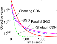
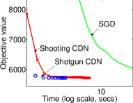
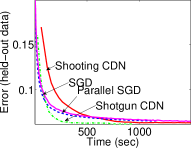
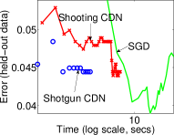
Fig. 4 plots training objectives and test accuracy (on a held-out of the data) for two large datasets.
The zeta dataset 555The zeta dataset is from the Pascal Large Scale Learning Challenge: http://www.mlbench.org/instructions/ illustrates the regime with . It contains 500K samples with 2000 features and is fully dense (in ). SGD performs well and is fairly competitive with Shotgun CDN (with ).
The rcv1 dataset 666Our version of the rcv1 dataset is from the LIBSVM repository (Chang & Lin, 2001). (Lewis et al., 2004) illustrates the high-dimensional regime (). It has about twice as many features (44504) as samples (18217), with non-zeros in . Shotgun CDN () was much faster than SGD, especially in terms of the objective. Parallel SGD performed almost identically to SGD.
Though convergence bounds for SMIDAS are comparable to those for SGD, SMIDAS iterations take much longer due to the mirror descent updates. To execute 10M updates on the zeta dataset, SGD took 728 seconds, while SMIDAS took over 8500 seconds.
These results highlight how SGD is orthogonal to Shotgun: SGD can cope with large , and Shotgun can cope with large . A hybrid algorithm might be scalable in both and and, perhaps, be parallelized over both samples and features.
 |
 |
 |
 |
| zeta with | rcv1 with |
4.3 Self-Speedup of Shotgun
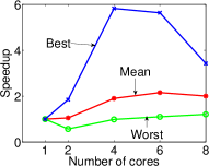
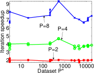
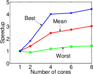
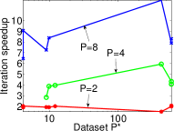
To study the self-speedup of Shotgun Lasso and Shotgun CDN, we ran both solvers on our datasets with varying , using varying (number of parallel updates = number of cores). We recorded the running time as the first time when an algorithm came within of the optimal objective, as computed by Shooting.
Fig. 5 shows results for both speedup (in time) and speedup in iterations until convergence. The speedups in iterations match Theorem 3.2 quite closely. However, relative speedups in iterations (about ) are not matched by speedups in runtime (about to ).
We thus discovered that speedups in time were limited by low-level technical issues. To understand the limiting factors, we analyzed various Shotgun-like algorithms to find bottlenecks.777See the supplement for the scalability analysis details. We found we were hitting the memory wall (Wulf & McKee, 1995); memory bus bandwidth and latency proved to be the most limiting factors. Each weight update requires an atomic update to the shared vector, and the ratio of memory accesses to floating point operations is only . Data accesses have no temporal locality since each weight update uses a different column of . We further validated these conclusions by monitoring CPU counters.
 |
 |
 |
 |
| (a) Shotgun Lasso | (b) Shotgun Lasso | (c) Shotgun CDN | (d) Shotgun CDN |
| runtime speedup | iterations | runtime speedup | iterations |
5 Discussion
We introduced the Shotgun, a simple parallel algorithm for -regularized optimization. Our convergence results for Shotgun are the first such results for parallel coordinate descent with regularization. Our bounds predict linear speedups, up to an interpretable, problem-dependent limit. In experiments, these predictions matched empirical behavior.
Extensive comparisons showed that Shotgun outperforms state-of-the-art solvers on many datasets. We believe that, currently, Shotgun is one of the most efficient and scalable solvers for -regularized problems.
The most exciting extension to this work might be the hybrid of SGD and Shotgun discussed in Sec. 4.3.
Code, Data, and Benchmark Results: Available at http://www.select.cs.cmu.edu/projects
Acknowledgments
Thanks to John Langford, Guy Blelloch, Joseph Gonzalez, Yucheng Low
and our reviewers for feedback.
Funded by NSF IIS-0803333, NSF CNS-0721591, ARO MURI W911NF0710287,
ARO MURI W911NF0810242.
References
- Blumensath & Davies (2009) Blumensath, T. and Davies, M.E. Iterative hard thresholding for compressed sensing. Applied and Computational Harmonic Analysis, 27(3):265–274, 2009.
- Chang & Lin (2001) Chang, C.-C. and Lin, C.-J. LIBSVM: a library for support vector machines, 2001. http://www.csie.ntu.edu.tw/~cjlin/libsvm.
- Duarte et al. (2008) Duarte, M.F., Davenport, M.A., Takhar, D., Laska, J.N., Sun, T., Kelly, K.F., and Baraniuk, R.G. Single-pixel imaging via compressive sampling. Signal Processing Magazine, IEEE, 25(2):83–91, 2008.
- Efron et al. (2004) Efron, B., Hastie, T., Johnstone, I., and Tibshirani, R. Least angle regression. Annals of Statistics, 32(2):407–499, 2004.
- Figueiredo et al. (2008) Figueiredo, M.A.T, Nowak, R.D., and Wright, S.J. Gradient projection for sparse reconstruction: Application to compressed sensing and other inverse problems. IEEE J. of Sel. Top. in Signal Processing, 1(4):586–597, 2008.
- Friedman et al. (2010) Friedman, J., Hastie, T., and Tibshirani, R. Regularization paths for generalized linear models via coordinate descent. Journal of Statistical Software, 33(1):1–22, 2010.
- Fu (1998) Fu, W.J. Penalized regressions: The bridge versus the lasso. J. of Comp. and Graphical Statistics, 7(3):397–416, 1998.
- Kim et al. (2007) Kim, S. J., Koh, K., Lustig, M., Boyd, S., and Gorinevsky, D. An interior-point method for large-scale 1-regularized least squares. IEEE Journal of Sel. Top. in Signal Processing, 1(4):606–617, 2007.
- Kogan et al. (2009) Kogan, S., Levin, D., Routledge, B.R., Sagi, J.S., and Smith, N.A. Predicting risk from financial reports with regression. In Human Language Tech.-NAACL, 2009.
- Koh et al. (2007) Koh, K., Kim, S.-J., and Boyd, S. An interior-point method for large-scale l1-regularized logistic regression. JMLR, 8:1519–1555, 2007.
- Langford et al. (2009a) Langford, J., Li, L., and Zhang, T. Sparse online learning via truncated gradient. In NIPS, 2009a.
- Langford et al. (2009b) Langford, J., Smola, A.J., and Zinkevich, M. Slow learners are fast. In NIPS, 2009b.
- Leiserson (2009) Leiserson, C. E. The Cilk++ concurrency platform. In 46th Annual Design Automation Conference. ACM, 2009.
- Lewis et al. (2004) Lewis, D.D., Yang, Y., Rose, T.G., and Li, F. RCV1: A new benchmark collection for text categorization research. JMLR, 5:361–397, 2004.
- Mann et al. (2009) Mann, G., McDonald, R., Mohri, M., Silberman, N., and Walker, D. Efficient large-scale distributed training of conditional maximum entropy models. In NIPS, 2009.
- Ng (2004) Ng, A.Y. Feature selection, vs. regularization and rotational invariance. In ICML, 2004.
- Shalev-Shwartz & Tewari (2009) Shalev-Shwartz, S. and Tewari, A. Stochastic methods for regularized loss minimization. In ICML, 2009.
- Strang (1988) Strang, G. Linear Algebra and Its Applications. Harcourt Brace Jovanovich, 3rd edition, 1988.
- Tibshirani (1996) Tibshirani, R. Regression shrinkage and selection via the lasso. J. Royal Statistical Society, 58(1):267–288, 1996.
- Tsitsiklis et al. (1986) Tsitsiklis, J. N., Bertsekas, D. P., and Athans, M. Distributed asynchronous deterministic and stochastic gradient optimization algorithms. 31(9):803–812, 1986.
- van den Berg et al. (2009) van den Berg, E., Friedlander, M.P., Hennenfent, G., Herrmann, F., Saab, R., and Yılmaz, O. Sparco: A testing framework for sparse reconstruction. ACM Transactions on Mathematical Software, 35(4):1–16, 2009.
- Wen et al. (2010) Wen, Z., Yin, W. Goldfarb, D., and Zhang, Y. A fast algorithm for sparse reconstruction based on shrinkage, subspace optimization and continuation. SIAM Journal on Scientific Computing, 32(4):1832–1857, 2010.
- Wright et al. (2009) Wright, S.J., Nowak, D.R., and Figueiredo, M.A.T. Sparse reconstruction by separable approximation. IEEE Trans. on Signal Processing, 57(7):2479–2493, 2009.
- Wulf & McKee (1995) Wulf, W.A. and McKee, S.A. Hitting the memory wall: Implications of the obvious. ACM SIGARCH Computer Architecture News, 23(1):20–24, 1995.
- Yuan et al. (2010) Yuan, G. X., Chang, K. W., Hsieh, C. J., and Lin, C. J. A comparison of optimization methods and software for large-scale l1-reg. linear classification. JMLR, 11:3183–3234, 2010.
- Zinkevich et al. (2010) Zinkevich, M., Weimer, M., Smola, A.J., and Li, L. Parallelized stochastic gradient descent. In NIPS, 2010.