Nonlinear Biasing and Redshift-Space Distortions in Lagrangian Resummation Theory and N-body Simulations

Abstract

Understanding a behavior of galaxy biasing is crucial for future galaxy redshift surveys. One aim is to measure the baryon acoustic oscillations (BAOs) within the precision of a few percent level. Using 30 large cosmological $N$-body simulations for a standard $\Lambda$CDM cosmology, we study the halo biasing over a wide redshift range. We compare the simulation results with theoretical predictions proposed by Matsubara which naturally incorporate the halo bias and redshift-space distortions into their formalism of perturbation theory with a resummation technique via the Lagrangian picture. The power spectrum and correlation function of halos obtained from Lagrangian resummation theory (LRT) well agree with $N$-body simulation results on scales of BAOs. Especially nonlinear effects on the baryon acoustic peak of the halo correlation function are accurately explained both in real and redshift space. We find that nonlinearity and scale dependence of bias are fairly well reproduced by 1-loop LRT up to $k=0.35h$Mpc^-1 ($z=2$ and 3) within a few percent level in real space and up to $k=0.1h$Mpc^-1 ($z=2$) and 0.15$h$Mpc^-1 ($z=$3) in redshift space. Thus, the LRT is very powerful for accurately extracting cosmological information in upcoming high redshift BAO surveys.

I Introduction

The redshift survey of galaxies is one of the most important methods to probe the nature of a mysterious energy component called dark energy, which is supposed to explain the late-time cosmic acceleration discovered by the observation of distant supernovae (Riess et al., 1998; Perlmutter et al., 1999). Baryon acoustic oscillations (BAOs) imprinted on the large scale structure can be used as a standard ruler to measure the cosmic expansion history of the Universe (e.g., Blake and Glazebrook, 2003; Hu and Haiman, 2003; Seo and Eisenstein, 2003; Glazebrook and Blake, 2005; Seo and Eisenstein, 2007). The characteristic scale of BAOs, which is determined by the sound horizon scale of baryon-photon plasma at the recombination epoch, is though to be a robust measure (e.g., Eisenstein et al., 1998; Cooray et al., 2001; Hu, 2005). Using the BAOs as a standard ruler, large galaxy surveys are expected to provide a tight constraint on the nature of dark energy (e.g., Linder, 2003; Matsubara, 2004; Amendola et al., 2005; Albrecht et al., 2006; Dolney et al., 2006; Albrecht et al., 2009).

That is why most of the planned galaxy redshift surveys aim at measuring BAOs within the precision of a few percent level. Some examples are BigBOSS (Schlegel et al., 2009), Euclid (Refregier et al., 2010), the Hobby-Eberly Telescope Dark Energy Experiment (HETDEX), the Large Sky Area Multi-Object Fiber Spectroscopic Telescope (LAMOST), the Square Kilometre Array (SKA), the Subaru Measurement of Images and Redshifts (SuMIRe) and the Wide-Field Infrared Survey Telescope (WFIRST). Recent observations of BAOs in modern galaxy surveys work well and constrain the cosmological parameters with approximately 10% level (see, e.g., Cole et al., 2005; Eisenstein et al., 2005; Tegmark et al., 2006; Padmanabhan et al., 2007; Percival et al., 2007; Okumura et al., 2008; Reid et al., 2010).

However, in order to pursue an order-of-magnitude improvement, a theoretically precise description of the BAOs is a crucial issue. It needs to be investigated taking account of the various systematic effects. The two main systematic effects are galaxy biasing and redshift-space distortions. The spatial pattern of galaxy distribution is not the same as that of dark matter and the galaxies are biased tracers of mass (Kaiser, 1984; Bardeen et al., 1986). The redshift of a galaxy does not purely reflect the Hubble flow, and Doppler shift by a peculiar velocity is inevitably added. Therefore the spatial pattern of clustering of galaxies is distorted in redshift space (Kaiser, 1987). With time, these effects are increasingly difficult to treat due to nonlinear evolution of structure growth and degrade the contrast of the BAOs in the matter power spectrum and/or correlation function, decreasing the signal-to-noise ratio of the standard ruler method. The nonlinear effects on BAOs play an important role in taking into account percent-level cosmology although baryonic features appear on large scales such as $100h^{-1}$Mpc. The amplitude of BAOs is increasingly damped from small scales to large scales, with decreasing redshift (e.g., Meiksin et al., 1999; Seo and Eisenstein, 2005; Eisenstein et al., 2007; Huff et al., 2007; Seo et al., 2008; Smith et al., 2008a; Padmanabhan and White, 2009; Seo et al., 2010; Mehta et al., 2011). Redshift distortion effects enhance a nonlinear damping of BAOs along the line-of-sight direction (e.g., Meiksin et al., 1999; Seo and Eisenstein, 2005; Eisenstein et al., 2007; Huff et al., 2007; Seo et al., 2008; Smith et al., 2008a; Padmanabhan and White, 2009; Seo et al., 2010; Mehta et al., 2011). Biasing is also affected by nonlinear effects and is scale dependent on BAOs scales. Such nonlinear effects impose a serious problem in analyzing galaxy surveys (e.g., Blanton et al., 2006; Smith et al., 2007; Percival et al., 2007; Sánchez and Cole, 2008; Blake et al., 2011).

Since galaxies are expected to form within dark matter halos, understanding and modeling the clustering properties of the halos play an important role in model galaxy biasing. In the usual halo model approach, the halo clustering is modeled by linear dynamics and linear bias factors (Mo and White, 1996; Peacock and Smith, 2000; Seljak, 2000; Cooray and Sheth, 2002). Recently, Smith et al. (2007); Smith et al. (2008b) and Elia et al. (2010) developed a nonlinear perturbation theory, incorporating the effects of halo bias. In their approach, there are some problems. Smith et al. (2007); Smith et al. (2008b) treat the halo bias as a local bias in Eulerian space, although the halo bias is intrinsically nonlocal in Eulerian space and does not fit well into the local Eulerian biasing scheme (Matsubara, 2011). Meanwhile, the analytic approach developed by Elia et al. (2010) cannot deal with the redshift-space distortions.

In this paper, we use nonlinear perturbation theory developed by Matsubara (2008a) which naturally incorporate the halo bias and redshift-space distortions in their formalism of perturbation theory with a resummation technique through the Lagrangian picture. A significant advantage of the Lagrangian resummation theory (LRT) is that it is simpler and easier to calculate the power spectrum than other resummation methods even in the presence of halo bias and redshift-space distortions. The computational cost is similar to that of standard perturbation theory (SPT) (e.g., Bernardeau et al., 2002). In this work, we examine how well it reproduces the simulation results in both real and redshift space. We focus not only on the halo power spectrum but also on the halo correlation function, because cosmological information that can be extracted from them is not exactly equivalent to each other because of different error properties. In this paper, we use 1-loop LRT for simplicity. The 2-loop corrections should be useful to extend the valid range, once we confirm that the 1-loop results agree with simulations (Okamura et al., 2011).

The structure of this paper is as follows. In Section. II, we briefly review analytical models in order to obtain matter power spectrum in real and redshift space. We also review the halo power spectrum based on 1-loop LRT. In Section. III we describe the details of $N$-body simulation and a method to calculate the power spectrum and two-point correlation function from $N$-body simulations. In Section. IV we show the main results. Section V is devoted to our conclusions.

II Analytical Models

There are several analytical models to account for evolutions of the matter power spectra in real and redshift space. In this paper, we mainly use three analytical models to compare the $N$-body simulation results; Linear perturbation theory (LIN) (e.g., Padmanabhan, 1993), 1-loop SPT (e.g., Bernardeau et al., 2002), and 1-loop LRT (e.g., Buchert, 1989, 1992; Buchert and Ehlers, 1993; Buchert, 1994; Catelan, 1995; Hivon et al., 1995; Ehlers and Buchert, 1997; Tatekawa, 2004; Matsubara, 2008b).

II.1 Matter power spectra in real space

Assuming that the amplitude of fluctuation is small, we can derive SPT as expansion of the fluid equations. Schematically, the expansion is written as

$$P_{\rm SPT}(k,z)=D_{+}(z)^{2}P_{\rm L,0}(k)+D_{+}(z)^{4}P_{\rm SPT,0}^{\mbox{\scriptsize 1-loop}}(k)+\cdots,$$ (1)

where $D_{+}(z)$ is the linear growth factor normalized to unity at present and $P_{\rm L,0}(k)$ and $P_{\rm SPT,0}^{\mbox{\scriptsize 1-loop}}(k)$ are the linear power spectrum and the 1-loop contribution to power spectrum, respectively, at present. For the sake of convenience, by using $P_{\rm L}(k,z)\equiv D_{+}(z)^{2}P_{\rm L,0}(k)$ and $P_{\rm SPT}^{\mbox{\scriptsize 1-loop}}(k,z)\equiv D_{+}(z)^{4}P_{\rm SPT,0}^{\mbox{\scriptsize 1-loop}}(k)$, we rewrite Eq. (1) as

$$P_{\rm SPT}(k)=P_{\rm L}(k)+P_{\rm SPT}^{\mbox{\scriptsize 1-loop}}(k)+\cdots.$$ (2)

Here we drop the $z$ dependence. Throughout this paper, we do not write the $z$ dependence unless otherwise stated. The explicit expressions of the 1-loop contribution can be found in the literature (e.g., Suto and Sasaki, 1991; Makino et al., 1992; Jain and Bertschinger, 1994; Nishimichi et al., 2007; Carlson et al., 2009).

On the other hand, 1-loop LRT is written as (Matsubara, 2008b)

$$P_{\rm LRT}(k)=\exp\left(-k^{2}\sigma_{\rm v}^{2}\right)\left[P_{\rm SPT}(k)+k^{2}\sigma_{\rm v}^{2}P_{\rm L}(k)\right],$$ (3)

in terms of SPT. Here $\sigma_{\rm v}^{2}$ is the one-dimensional linear velocity dispersion given by

$$\sigma_{\rm v}^{2}=\frac{1}{3}\int\frac{{\rm d}^{3}\vec{p}}{(2\pi)^{3}}\frac{P_{\rm L}(p)}{p^{2}}.$$ (4)

If the exponential prefactor is expanded, the 1-loop SPT is exactly recovered when we consider the 1-loop level.

Finally we comment on other perturbation theories. Several other approaches have been proposed beyond SPT, such as the renormalized perturbation theory (RPT) (Crocce and Scoccimarro, 2006a, b, 2008), the large-$N$ expansion (Valageas, 2007), the Time-RG method (Pietroni, 2008), the renormalization group approach (Matarrese and Pietroni, 2008) and the closure theory (Taruya and Hiramatsu, 2008). In these newly developed approaches, the standard perturbative expansion is reorganized and partially resummed in various ways. Different levels of approximations and ansatz are used in those approaches.

II.2 Matter power spectra in redshift space

As in real space, we use SPT and LRT in redshift space. Schematically, SPT in redshift space is written as

$$P_{\rm SPT}^{\rm s}(k,\mu)=(1+f\mu^{2})^{2}P_{\rm L}(k)+P_{\rm SPT}^{\mbox{\scriptsize s,1-loop}}(k,\mu)+\cdots,$$ (5)

where $f=d\ln{D}/d\ln{a}$ is the logarithmic derivative of the linear growth rate and $\mu$ is the cosine of the angle between the line of sight and the wave vector $\vec{k}$. Here $P_{\rm SPT}^{\mbox{\scriptsize s,1-loop}}(k)$ is the 1-loop contribution to the redshift-space power spectrum in SPT (Matsubara, 2008b). The first term on the right-hand side is the linear-order result of the redshift-space power spectrum and the factor $(1+f\mu^{2})^{2}$ indicates the enhancement of the power spectrum which is the so-called Kaiser effect (Kaiser, 1987). The Kaiser effect is represented as the coherent distortion by a peculiar velocity along the line-of-sight direction.

On the other hand, 1-loop LRT in redshift space is written as (Matsubara, 2008b)

$$P_{\rm LRT}^{\rm s}(k,\mu) =\exp\left[-k^{2}\sigma_{\rm v}^{2}[1+f(f+2)\mu^{2}]\right]$$

$$\times\Bigl{[}(1+f\mu^{2})^{2}P_{\rm L}(k)+P_{\rm SPT}^{\mbox{\scriptsize s,1-loop}}(k,\mu)$$

$$+(1+f\mu^{2})^{2}[1+f(f+2)\mu^{2}]k^{2}\sigma_{\rm v}^{2}P_{\rm L}(k)\Bigr{]},$$ (6)

As in the case in real space, if the exponential prefactor is expanded, Eq. (6) reduces to the 1-loop SPT result. The exponential prefactor shows the nonlinear damping effect by the random motion of peculiar velocities, i.e., the Fingers-of-God effect (Jackson, 1972; Sargent and Turner, 1977).

We also use a model of redshift-space power spectrum, proposed by Scoccimarro (2004). This model gives

$$P_{\rm SCO}^{\rm s}(k,\mu) =\exp\left(-f^{2}\mu^{2}k^{2}\sigma_{\rm v}^{2}\right)$$

$$\times\left[P_{\delta\delta}(k)+2f\mu^{2}P_{\delta\theta}(k)+f^{2}\mu^{4}P_{\theta\theta}\right],$$ (7)

where $P_{\delta\delta}(k)$, $P_{\theta\theta}(k)$ and $P_{\delta\theta}(k)$ are auto power spectra of density and velocity, and their cross power spectrum, respectively. This model accounts for the nonlinear effects although it is still phenomenological.

In this paper, we consider only the monopole power spectrum which is defined as

$$P^{\rm s}(k)=\frac{1}{2}\int_{-1}^{1}{\rm d}{\mu}P^{\rm s}(k,\mu).$$ (8)

Other multipole contributions to the power spectrum and correlation function in redshift space, such as the quadrupole and hexadecapole are examined in the literature (e.g., Hamilton, 1998; Tinker et al., 2006; Taruya et al., 2009, 2010; Kazin et al., 2011; Kwan et al., 2011; Reid and White, 2011; Tang et al., 2011; Taruya et al., 2011).

II.3 Halo power spectra in real and redshift space

Based on 1-loop LRT, the power spectrum of the biased object in redshift space is given by (Matsubara, 2008a)

$$P_{\rm hh,LRT}^{\rm s}(k,\mu) =\exp\left[-k^{2}\sigma_{\rm v}^{2}[1+f(f+2)\mu^{2}]\right]\Bigl{[}(1+\langle{F^{\prime}}\rangle$$

$$+f\mu^{2})^{2}P_{\rm L}(k)+\sum_{n,m}\mu^{2n}f^{m}E_{nm}(k)\Bigr{]},$$ (9)

where $\langle{F^{\prime}}\rangle$ denotes a Lagrangian linear bias factor and the explicit expression of $E_{nm}(k)$ is shown in Matsubara (2008a). $E_{nm}(k)$ includes the higher-order Lagrangian bias factor such as $\langle{F^{\prime\prime}}\rangle$. Up to 1-loop order, we need only two bias factors $\langle{F^{\prime}}\rangle$ and $\langle{F^{\prime\prime}}\rangle$. When we consider a mass range [$M_{1}$, $M_{2}$] of halos, the bias function for the halo bias is given by (Matsubara, 2008a)

$$\langle{F^{(n)}}\rangle=\frac{(-1)^{n}}{\delta_{c}^{n}}\frac{\int_{M_{1}}^{M_{2}}\nu^{n}\frac{{\rm d}^{n}g}{{\rm d}\nu^{n}}\frac{{\rm d}\ln\sigma}{{\rm d}{M}}\frac{{\rm d}{M}}{M}}{\int_{M_{1}}^{M_{2}}g(\nu)\frac{{\rm d}\ln\sigma}{{\rm d}{M}}\frac{{\rm d}{M}}{M}},$$ (10)

where $\delta_{c}$ is the critical overdensity at the present time. In an Einstein-de Sitter cosmology, $\delta_{c}=1.686$. For general cosmology, the value of $\delta_{c}$ shows weak dependence on cosmology (Lacey and Cole, 1993; Eke et al., 1996; Nakamura and Suto, 1997; Henry, 2000), so we include cosmological dependence on $\delta_{c}$. The quantity $\sigma$ is the root-mean-square linear density smoothed with a top hat filter of radius $R$ and enclosing an average mass $M=\rho_{0}4\pi{R}^{3}/3$,

$$\sigma^{2}(M)=\int\frac{k^{2}{\rm d}{k}}{2\pi^{2}}W^{2}(kR)P_{\rm L}(k),$$ (11)

with

$$W(x)=\frac{3}{x^{3}}(\sin x-x\cos x),$$ (12)

where $\rho_{0}$ is the mean matter density of the Universe. The quantity $\nu$ is defined by $\nu=\delta_{c}/\sigma$. $g(\sigma)$ is the scaled differential mass function defined as (Jenkins et al., 2001)

$$g(\sigma)=\frac{M}{\rho_{0}}\frac{{\rm d}{n}}{{\rm d}\ln\sigma^{-1}},$$ (13)

where $n$ is the number density of halos with mass $M$. The quantity $g(\sigma)$ is frequently used in the literature and there have been several analytical predictions (Press and Schechter, 1974; Bond et al., 1991; Sheth et al., 2001) and fitting formulae (e.g., Sheth and Tormen, 1999; Jenkins et al., 2001; Warren et al., 2006; Reed et al., 2007; Crocce et al., 2010; Manera et al., 2010; Bhattacharya et al., 2011) for $g(\sigma)$. In section IV.3, we will compare the mass function obtained from our $N$-body simulations with several fitting formulae to examine which fitting formulae are better.

From Eq. (9) with substituting $f=0$, the power spectrum of the biased object based on 1-loop LRT in real space is obtained as

$$P_{\rm hh,LRT}(k)=\exp\left[-k^{2}\sigma_{\rm v}^{2}\right]\left[(1+\langle{F^{\prime}}\rangle)^{2}P_{\rm L}(k)+E_{00}(k)\right].$$ (14)

By expanding the exponential prefactor and considering the linear term in $P_{\rm L}(k)$, the linear result is derived as

$$P_{\rm hh,LIN}(k)=(1+\langle{F^{\prime}}\rangle)^{2}P_{\rm L}(k).$$ (15)

In linear theory, using the Eulerian linear bias factor $b$, the power spectrum of the biased object is defined by

$$P_{\rm hh,LIN}(k)=b^{2}P_{\rm L}(k).$$ (16)

Comparing Eq. (15) and Eq. (16), we can easily derive the relation between Eulerian and Lagrangian biases as

$$b=1+\langle{F^{\prime}}\rangle.$$ (17)

This result is the same as that derived from the halo model approach by using the spherical collapse model (Mo and White, 1996; Mo et al., 1997), i.e., the Eulerian linear bias is given by unity plus the Lagrangian linear bias (see, (Matsubara, 2011) for more accurate expressions on nonlinear scales). It should be noted that the result of Eq. (17) is derived without assuming a spherical collapse model.

The corresponding linear result in redshift space is obtained by a linear term of Eq. (9) as

$$P_{\rm hh,LIN}^{\rm s}(k,\mu)=(1+\langle{F^{\prime}}\rangle+f\mu^{2})^{2}P_{\rm L}(k).$$ (18)

By using Eq. (17), this equation is rewritten by

$$P_{\rm hh,LIN}^{\rm s}(k,\mu)=b^{2}(1+\beta\mu^{2})^{2}P_{\rm L}(k),$$ (19)

where $\beta=f/b$ is the redshift-space distortion parameter. This equation is equivalent to the Kaiser formula (Kaiser, 1987). Methods used to determine the redshift-space distortion parameter $\beta$ are summarized by Hamilton (1998).

III $N$-body Simulations

III.1 Simulation Parameters

Table 1: Parameters used in low- and high-resolution $N$-body simulations.

Name	$\Omega_{\rm m}$	$\Omega_{\Lambda}$	$\Omega_{\rm b}$	$h$	$n_{s}$	$\sigma_{8}$	$L_{\rm box}$	$N_{p}$	$z_{\rm ini}$	$r_{\rm s}$	$N_{\rm run}$
L1000(low resolution)	0.265	0.735	0.0448	0.71	0.963	0.80	1000$h^{-1}$Mpc	10243	36	50$h^{-1}$kpc	30
L500(high resolution)	0.265	0.735	0.0448	0.71	0.963	0.80	500$h^{-1}$Mpc	10243	42	25$h^{-1}$kpc	5

We use the numerical simulation code Gadget2 (Springel, 2005) in its full tree-particle mesh mode. For all of the simulations discussed in the present paper, we adopted the standard $\Lambda$CDM model with the matter density $\Omega_{m}=0.265$, baryon density $\Omega_{b}=0.0448$, dark energy density $\Omega_{\Lambda}=0.735$ with equation of state parameter $w=-1$, spectral index $n_{s}=0.963$, the variance of the density fluctuation in a sphere of radius 8 $h^{-1}$Mpc $\sigma_{8}=0.80$, and Hubble parameter $h=0.71$. These cosmological parameters are consistent with the Wilkinson Microwave Anisotropy Probe 7yr (WMAP7) results (Komatsu et al., 2011). We employ $N_{p}=1024^{3}$ particles in boxes of side $L_{\rm box}=1000h^{-1}$Mpc with softening length $r_{\rm s}$ being $50h^{-1}$kpc and of side $L_{\rm box}=500h^{-1}$Mpc with softening length $r_{\rm s}$ being $25h^{-1}$kpc, respectively abbreviated to L1000 and L500. Throughout this paper, we show results obtained from L1000 unless otherwise stated. The initial conditions are generated based on the 2nd-order Lagrangian perturbation theory (2LPT) (Crocce et al., 2006; Nishimichi et al., 2009) with the initial linear power spectrum calculated by CAMB (Lewis et al., 2000). We use parallelized 2LPT code which is kindly provided by Takahiro Nishimichi who developed it in Valageas and Nishimichi (2011) to run large cosmological $N$-body simulations with initial conditions based on 2LPT. The initial redshift is set to $z_{\rm ini}=36$ for L1000 and $z_{\rm ini}=42$ for L500. We perform $N_{\rm run}=30$ realizations for L1000 and $N_{\rm run}=5$ realizations for L500. Table 1 summarizes the parameters used in the simulations.

Table 2: Properties of halo catalogues for low- and high-resolution simulations. $\bar{N}_{h}$, $\bar{n}_{h}$ and $\bar{M}_{h}$ are the ensemble average number, number densities and mass of halos for redshifts we employed.

L1000(low resolution)				L500(high resolution)
	$\bar{N}_{h}$	$\bar{n}_{h}[h^{3}{\rm Mpc}^{-3}]$	$\bar{M}_{h}[h^{-1}M_{\odot}]$		$\bar{N}_{h}$	$\bar{n}_{h}[h^{3}{\rm Mpc}^{-3}]$	$\bar{M}_{h}[h^{-1}M_{\odot}]$
$z=3$	4.00$\times{10}^{5}$	4.00$\times{10}^{-4}$	2.59$\times{10}^{12}$	$z=3$	1.08$\times{10}^{6}$	8.68$\times{10}^{-3}$	4.58$\times{10}^{11}$
$z=2$	1.21$\times{10}^{6}$	1.21$\times{10}^{-3}$	3.30$\times{10}^{12}$	$z=2$	1.86$\times{10}^{6}$	1.48$\times{10}^{-2}$	6.12$\times{10}^{11}$
$z=1$	2.38$\times{10}^{6}$	2.38$\times{10}^{-3}$	4.75$\times{10}^{12}$	$z=1$	2.42$\times{10}^{6}$	1.94$\times{10}^{-2}$	9.07$\times{10}^{11}$
$z=0.5$	2.82$\times{10}^{6}$	2.82$\times{10}^{-3}$	5.99$\times{10}^{12}$	$z=0.5$	2.52$\times{10}^{6}$	2.01$\times{10}^{-2}$	1.15$\times{10}^{12}$
$z=0.3$	2.93$\times{10}^{6}$	2.93$\times{10}^{-3}$	6.63$\times{10}^{12}$	$z=0.3$	2.52$\times{10}^{6}$	2.01$\times{10}^{-2}$	1.27$\times{10}^{12}$
$z=0$	3.05$\times{10}^{6}$	3.05$\times{10}^{-3}$	7.73$\times{10}^{12}$	$z=0$	2.49$\times{10}^{6}$	1.99$\times{10}^{-2}$	1.47$\times{10}^{12}$

We store outputs at $z=3$, 2, 1, 0.5, 0.3, and 0 and identify halos for each output using a friends-of-friends (FOF) group finder with linking length of 0.2 times the mean separation (Davis et al., 1985). We select halos in which the number of particles, $N_{p}$, is equal to or larger than 20 which corresponds to the halos with masses $1.37\times 10^{12}h^{-1}M_{\odot}$ for L1000 and $1.71\times 10^{11}h^{-1}M_{\odot}$ for L500. The average number, number densities, and mass of halos among realizations for redshifts at which we store outputs can be found in Table 2.

III.2 Analysis: Power Spectra and Two-Point Correlation Functions

To calculate the power spectrum from $N$-body simulations, we calculate the Fourier transform of the density field, denoted as $\tilde{\delta}^{n}(\vec{k})$, where the superscript $n$ denotes the $n$-th realization and $\vec{k}$ shows the wave number. First, we assign the $N$-body particles onto $N_{\rm grid}^{3}=1024^{3}$ grids based on the cloud-in-cell (CIC) mass assignment scheme (Hockney and Eastwood, 1988). We then use Fast Fourier Transformation (FFT) to calculate the density contrast in Fourier space and correct the effect of the CIC mass assignment scheme as (Angulo et al., 2008; Takahashi et al., 2009)

$$\tilde{\delta}^{n}(\vec{k})\rightarrow\frac{\tilde{\delta}^{n}(\vec{k})}{\left[{\rm sinc}\left(\frac{k_{x}L_{\rm box}}{2N_{\rm grid}}\right){\rm sinc}\left(\frac{k_{y}L_{\rm box}}{2N_{\rm grid}}\right){\rm sinc}\left(\frac{k_{z}L_{\rm box}}{2N_{\rm grid}}\right)\right]^{2}},$$ (20)

where ${\rm sinc}(x)=\sin(x)/x$. A more careful analysis was done by Jing (2005). Finally, squaring the density contrast in Fourier space and taking an average over Fourier modes and realizations, the ensemble average of binned power spectrum is given by

$$\hat{P}(k_{i}) =\frac{1}{N_{\rm run}N_{i}^{k}}\sum_{n=1}^{N_{\rm run}}\sum_{k_{i}^{\rm min}<\lvert\vec{k}\rvert<k_{i}^{\rm max}}\left\lvert\tilde{\delta}^{n}(\vec{k})\right\rvert^{2},$$ (21)

$$k_{i} \equiv\frac{1}{N_{i}^{k}}\sum_{k_{i}^{\rm min}<\lvert\vec{k}\rvert<k_{i}^{\rm max}}\lvert\vec{k}\rvert,$$ (22)

where $N_{i}^{k}$ is the number of Fourier modes in the $i$-th wave number bin, and $k_{i}^{\rm min}$ and $k_{i}^{\rm max}$ are the minimum and maximum wave number of the $i$-th bin, respectively. The obtained power spectrum is contaminated by the shot noise effect due to the discreteness of density field in $N$-body simulations. We simply assume the Poisson model where the shot noise is given by the inverse of number density of dark matter particles, $1/\bar{n}=L_{\rm box}^{3}/N_{p}$ and then subtract the shot noise, though this effect is very small and only has an impact on the result at $z=3$ on scales we have considered. Note that the power spectra measured from the treatment above suffer from the effect of finite-mode sampling due to a finite number of realizations or a finite box size, shown by Takahashi et al. (2008). The finite-mode effect is important at $k\lower 2.15277pt\hbox{$\;\buildrel<\over{\sim}\;$}0.1h{\rm Mpc^{-1}}$. We do not eliminate finite-mode effect because extension of their method to the halo case we are interested in is not trivial. Hence, to overcome this effect we run many realizations, i.e., $N_{\rm run}=30$ and use a large simulation box size, i.e., $L_{\rm box}=1000h^{-1}{\rm Mpc}$.

To calculate the two-point correlation function from $N$-body simulations, we adopt the grid-based calculation using FFT. Taruya et al. (2009) show a grid-based calculation with FFT almost coincides with the direct pair-count method (see, Appendix C in their paper). Since the grid-based calculation with FFT is computationally less expensive than the direct pair counting, we therefore adopt the grid-based calculation. It should be noted that the grid-based calculation is limited to scales larger than the grid size $r>L_{\rm box}/N_{\rm grid}$. In this method, we first compute the square of the density field in Fourier space on each grid. Then taking the inverse Fourier transformation and an average over distances and realizations, we can obtain the two-point correlation functions. This is expressed as (Taruya et al., 2009)

$$\hat{\xi}(r_{i})=\frac{1}{N_{\rm run}N_{i}^{r}}\sum_{n=1}^{N_{\rm run}}\sum_{r_{i}^{\rm min}<\lvert\vec{r}\rvert<r_{i}^{\rm max}}{\rm FFT}^{-1}\left[\left\lvert\tilde{\delta}^{n}(\vec{k})\right\rvert^{2};\vec{r}\right],$$ (23)

where ${\rm FFT}^{-1}$ denotes the inverse FFT of the square of the density field in Fourier space. Here, $N_{i}^{r}$ is the number of modes in the $i$-th distance bin, and $r_{i}^{\rm min}$ and $r_{i}^{\rm max}$ are the minimum and maximum distances of the $i$-th bin, respectively. We chose $r_{i}$ to be the center of the $i$-th bin, i.e., $r_{i}=(r_{i}^{\rm min}+r_{i}^{\rm max})/2$.

For the estimation of the halo power spectrum, we adopt the same method used for the power spectrum estimation to the halo cases, but apply the FOF halo mass correction as will be discussed in Section. IV.3. To be more precise, we impose Eq. (29) to halo particles when we assign the halo particles based on the CIC mass assignment scheme in order to introduce the FOF mass correction for $N$-body simulations. Then replacing $\tilde{\delta}^{n}$ with $\tilde{\delta}_{h}^{n}$, we do the same calculation described above [from Eqs. (20)-(22)] in order to obtain the halo power spectrum. $\tilde{\delta}_{h}^{n}$ is the density field of halos in Fourier space in the $n$-th realization.

There is one concern about shot noise. If the dark matter halos are regarded as a Poisson sampling, the subtraction term is the same as the dark matter particle case but using the appropriate number density $\bar{n}_{h}$. However Smith et al. (2007) found that this standard correction method is not exactly correct for halos, particularly for those of large mass. This is probably because in order to identify halos by using the FOF algorithm, we automatically impose that distances between halos are larger than the sum of their radii, or they would have been linked as bigger halos. To correctly eliminate the shot noise, Smith et al. (2007) proposed a new procedure that includes this exclusion effect (see, Appendix A in their paper for more details and also see, Seljak et al. (2009); Hamaus et al. (2010) for a new method to suppress the shot noise effect by weighting halos). However, we do not use this procedure to subtract the shot noise, but use the standard correction method for simplicity. The result could not being changed on scales we are interested in, because the number density of halos are large enough, and there is little shot noise effect.

For the estimation of the halo two-point correlation function, we use a grid-based calculation with FFT as is used in matter correlation function.

IV Results

IV.1 Matter Power Spectra

Figure 1: Comparison of mass power spectra obtained from $N$-body simulations to analytical predictions in real (left panel) and redshift (right panel) space for redshifts, $z=3$, 2, 1, and 0.5 from top to bottom. Power spectra are normalized by the no-wiggle fitting formula $P_{\rm nw}(k)$ (Eisenstein and Hu, 1998) in real space and by the no-wiggle fitting formula taking the Kaiser effect into account $P^{s}_{\rm nw}(k)$ in redshift space, respectively. The solid, dotted and dashed curves show the predictions of the 1-loop Lagrangian resummation theory (1-loop LRT), the linear theory (LIN), and the 1-loop standard perturbation theory (1-loop SPT), respectively. The dot-dashed curves in the right panel show the predictions of the empirical model proposed by Scoccimarro (2004). The arrows indicate the valid ranges for several redshifts, where the results of 1-loop LRT are expected to be accurate within a few percent.

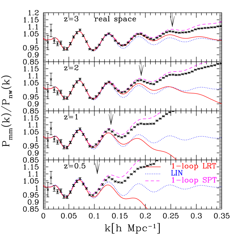
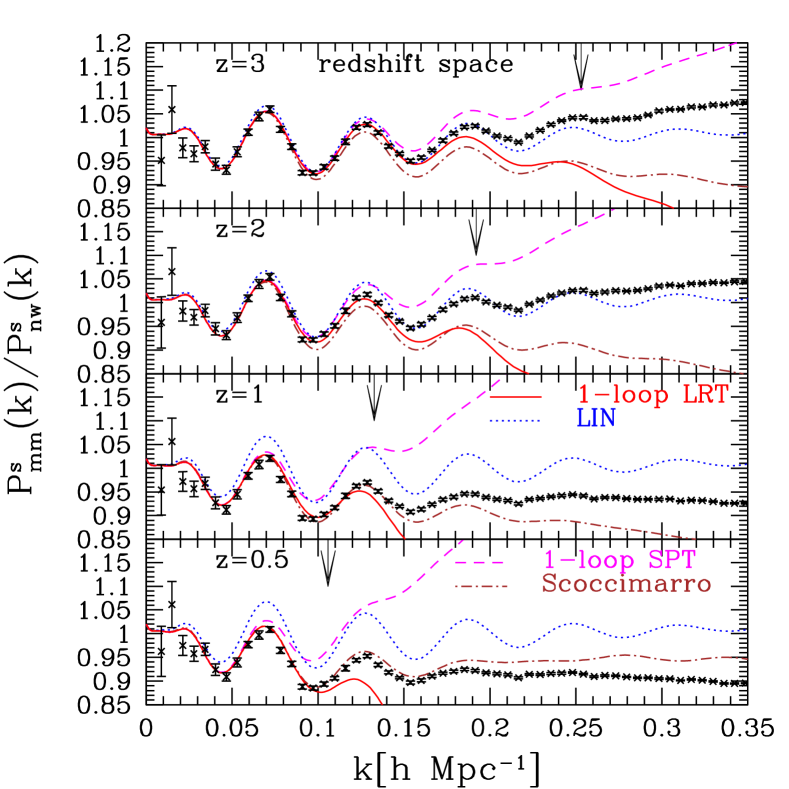
Figure 1 shows the matter power spectra obtained from $N$-body simulations among 30 realizations for $z=3$, 2, 1 and 0.5. We compare them with several analytical predictions. The left and right panels show the results of power spectrum divided by the smooth linear power spectrum $P_{\rm nw}(k)$ which is calculated by using the no-wiggle fitting formula of Eisenstein and Hu (1998) in real space and by the no-wiggle power spectrum taking the Kaiser effect ($1+2f/3+f^{2}/5$) into account in redshift space, respectively.

All of the theoretical predictions well agree with the $N$-body simulations within a range of the error bars on large scales. The range of agreement in all of the theoretical predictions is generally wider as redshift is higher. This is because the amplitude of density fluctuation is smaller at higher redshift. As has been stated in the literature (Carlson et al., 2009; Nishimichi et al., 2009), the result of 1-loop SPT (dashed curves) is not sufficiently accurate to describe the BAOs not only in real space but also in redshift space. It seems that the discrepancy in redshift space between the 1-loop SPT prediction and simulation results is larger than that in real space. The amplitude of the power spectrum from 1-loop SPT generally overestimates that from $N$-body simulations. However, the range of the agreement in 1-loop SPT is wider in both real and redshift space than that in LIN (dotted curves), because 1-loop SPT includes the next-order contribution of nonlinear growth. Meanwhile, the amplitude of the power spectrum in 1-loop LRT (solid curves) rapidly falls off at a certain wave number and it deviates from the $N$-body results. This is attributed to the exponential prefactor in Eqs. (3) and (6). In real space, the agreement of 1-loop LRT is roughly equivalent to that of 1-loop SPT. However, we can see that the 1-loop LRT results give a better agreement with simulations in redshift space. We also plot another theoretical prediction proposed by Scoccimarro (2004) in redshift space which is denoted as the dot-dashed curves in the right panel of Figure 1. The model of Scoccimarro (2004) seems to be a good agreement at certain redshift ($z=0.5$). However, this is just coincidence because it does not describe the simulation results at different redshifts.

Comparing the power spectra in real and redshift space, the amplitude of the power spectra on small scales in redshift space is suppressed by nonlinear redshift-space distortions. This suppression is due to the random motion of peculiar velocities in virialized objects which is known as the Fingers-of-God effect (Jackson, 1972; Sargent and Turner, 1977).

The arrows in Figure 1 indicate the reliable ranges $k_{\rm NL}/2$ for several redshifts, where the results of 1-loop LRT are expected to be accurate within a few percent. This criterion is proposed by Matsubara (2008b). It is determined by the damping scale of the exponent which is estimated from Eq. (4) as

$$k_{\rm NL}\equiv\frac{1}{\sigma_{\rm v}}=\left[\frac{1}{6\pi^{2}}\int{\rm d}{p}{P_{\rm L}}(p)\right]^{-1/2}.$$ (24)

IV.2 Correlation Functions

Figure 2: Comparison of two-point correlation functions obtained from $N$-body simulations to analytical predictions in real (left panel) and redshift (right panel) space for redshifts, $z=3$, 2, 1, 0.5, and 0 from bottom to top. The solid curves represent the results of the 1-loop Lagrangian resummation theory while the dotted curves show the results of the linear theory.

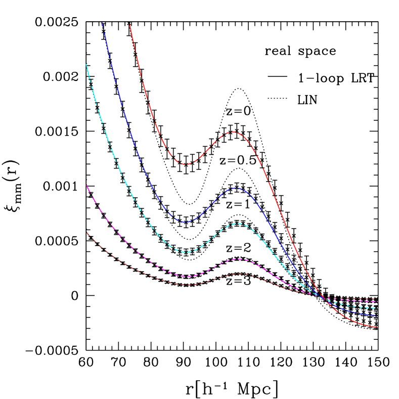
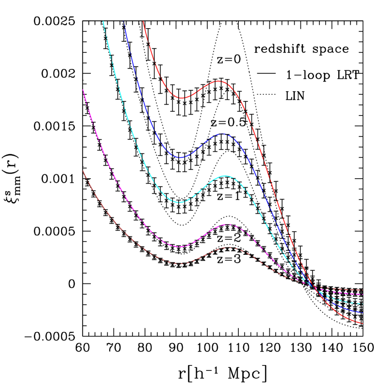
Next we focus on the two-point correlation function. Although the correlation function and power spectrum are directly related by Fourier transforms and have mathematically equivalent information, cosmological information that can be extracted from them with real data is not exactly equivalent because error properties are different. Therefore it is important to examine not only the power spectrum but also the two-point correlation function. Two-point correlation functions in real and redshift space around baryon acoustic peaks at $z=3$, 2, 1, 0.5, and 0 are shown in left and right panels of Figure 2, respectively. The theoretical two-point correlation function can be expressed in terms of the power spectrum as

$$\xi(r)=\int\frac{{k^{2}}{\rm d}{k}}{2\pi^{2}}\frac{\sin(kr)}{kr}P(k).$$ (25)

The $N$-body results clearly deviate from the LIN prediction (dotted curves) as decreasing the redshift, because nonlinear growth of the structure becomes significant as decreasing the redshift. In contrast, 1-loop LRT results (solid curves) fairly well reproduce the $N$-body results at all the redshift we have considered in both real and redshift space, although in redshift space a closer look around acoustic peaks reveals that the $N$-body results deviate from 1-loop LRT results as decreasing the redshift. Although the 1-loop LRT predictions considerably deviate from $N$-body simulation results on large wave number in the power spectrum (Figure 1), the acoustic peak structure in the correlation function comes from the low-$k$ behavior of the power spectrum, and the power spectrum at low-$k$ is accurately described by 1-loop LRT (Matsubara, 2008b; Sánchez et al., 2008).

The baryon acoustic peaks in both real and redshift space tend to be smeared as decreasing the redshift. However, the effect seems stronger than those in real space due to the Fingers-of-God effect. In the power spectrum results (Figure 1), the difference between 1-loop SPT and 1-loop LRT seems to be small, especially in real space. In correlation function results, however, the difference is quite big, because SPT cannot predict the correlation function which is ascribed to fail to convergence the integral in Eq. (25) (Matsubara, 2008b). Therefore, we conclude that the LRT is very powerful and sufficient to predict the BAOs in correlation functions.

IV.3 Halo Mass Functions

Figure 3: Halo mass function at redshift 0, 1 (left panel), 2 and 3 (right panel). We calculate the halo mass function from $N$-body simulations both with the force plus $N_{p}$ correction and without the correction (see text for correction in the details). The latter was shifted upward by a factor of 10 for clarity. The solid and dashed curves denote Bhattacharya et al. (2011) and Sheth and Tormen (1999) results, respectively.

If we want to accurately calculate the halo power spectra based on LRT, accurate halo mass functions are clearly needed, since the Lagrangian bias factor is expressed in terms of the halo mass function (see, Eq. 10). Here we use different mass function expressions given previously to compare our $N$-body simulation results. A famous numerical fit for $g(\sigma)$ is given by Sheth and Tormen (1999) (hereafter ST) which is expressed as

$$g_{\rm ST}(\sigma)=A\sqrt{\frac{2a}{\pi}}\left[1+\left(\frac{\sigma^{2}}{a\delta_{c}^{2}}\right)^{p}\right]\frac{\delta_{c}}{\sigma}\exp\left[-\frac{a\delta_{c}^{2}}{2\sigma^{2}}\right],$$ (26)

with $A=0.3222$, $a=0.707$ and $p=0.3$. Recently, Crocce et al. (2010) (hereafter MICE) recalibrated the halo mass function using a large set of $N$-body simulations with good mass resolution and large cosmological volumes called MICE simulations. They provided a numerical fit as

$$g_{\rm MICE}(\sigma)=A(z)\left[\sigma^{-a(z)}+b(z)\right]\exp\left[-\frac{c(z)}{\sigma^{2}}\right],$$ (27)

with $A(z)=0.58(1+z)^{-0.13}$, $a(z)=1.37(1+z)^{-0.15}$, $b(z)=0.3(1+z)^{-0.084}$, and $c(z)=1.036(1+z)^{-0.024}$. Bhattacharya et al. (2011) (hereafter Coyote) also recently recalibrated the mass function using their simulations so called as Coyote simulations whose parameters are very close to MICE simulations. Therefore, both results show good agreement within a few percent except at very high masses. The functional form of the Coyote fit which is similar to the ST mass function is expressed as

$$g_{\rm Coyote}(\sigma) =\tilde{A}\sqrt{\frac{2}{\pi}}\left[1+\left(\frac{\sigma^{2}}{\tilde{a}\delta_{c}^{2}}\right)^{\tilde{p}}\right]$$

$$\times\left(\frac{\delta_{c}\sqrt{\tilde{a}}}{\sigma}\right)^{\tilde{q}}\exp\left[-\frac{\tilde{a}\delta_{c}^{2}}{2\sigma^{2}}\right],$$ (28)

with $\tilde{A}=0.333(1+z)^{-0.11}$, $\tilde{a}=0.788(1+z)^{-0.01}$, $\tilde{p}=0.807$, and $\tilde{q}=1.795$.

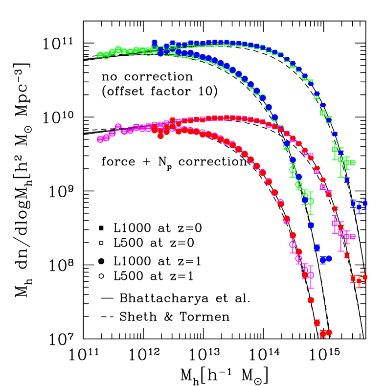
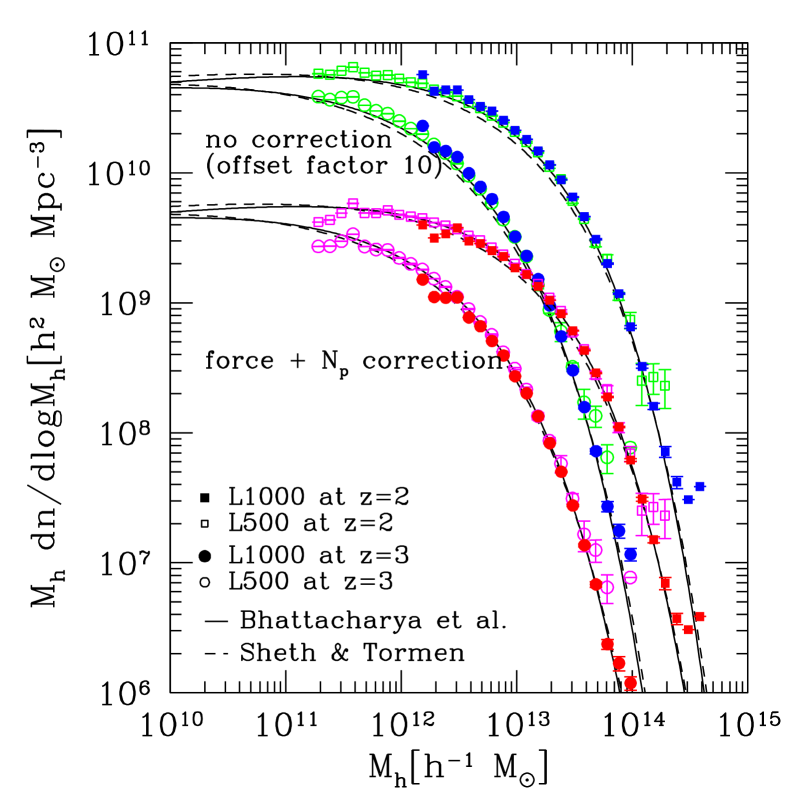
In Figure 3, we plot the halo mass function as a function of halo mass at $z=0$, 1, 2, and 3. We show the results of L1000 as filled symbols and the results of L500 as open symbols, respectively. The simulation results are plotted with the force plus the $N_{p}$ correction proposed by Bhattacharya et al. (2011) and without the correction. The latter was shifted upwards by a factor of 10 for visibility. The net correction for the FOF halo mass is expressed as (Bhattacharya et al., 2011)

$$M_{h}^{c}/M_{h}=[1.0-0.04(r_{s}/650{\rm kpc})](1-n_{h}^{-0.65}),$$ (29)

where $M_{h}^{c}$ is a corrected mass, $M_{h}$ is an uncorrected mass, and $n_{h}$ is the number of particles that construct a halos. This equation is slightly modified from the originally suggested equation by Warren et al. (2006):

$$M_{h}^{c}/M_{h}=1-n_{h}^{-0.60}.$$ (30)

The solid and dashed curves denote the results of Coyote and ST fitting formulae. Our simulation results well reproduce the Coyote results over a wide range of halo masses and redshifts, while ST slightly deviates from the simulation results, especially at large halo masses. The impact of the correction to the FOF mass can be easily seen in Figures 4 and 5.

Figure 4: The ratio of the halo mass function from $N$-body simulations to that from three fitting formulae: Sheth and Tormen (1999), Crocce et al. (2010), and Bhattacharya et al. (2011) for L500 (left panel) and L1000 (right panel). The upper and bottom panels show the results at redshift 1 and 0, respectively. The red and magenta symbols show the results with the force plus $N_{p}$ correction and the blue and green symbols show those without the correction, respectively.

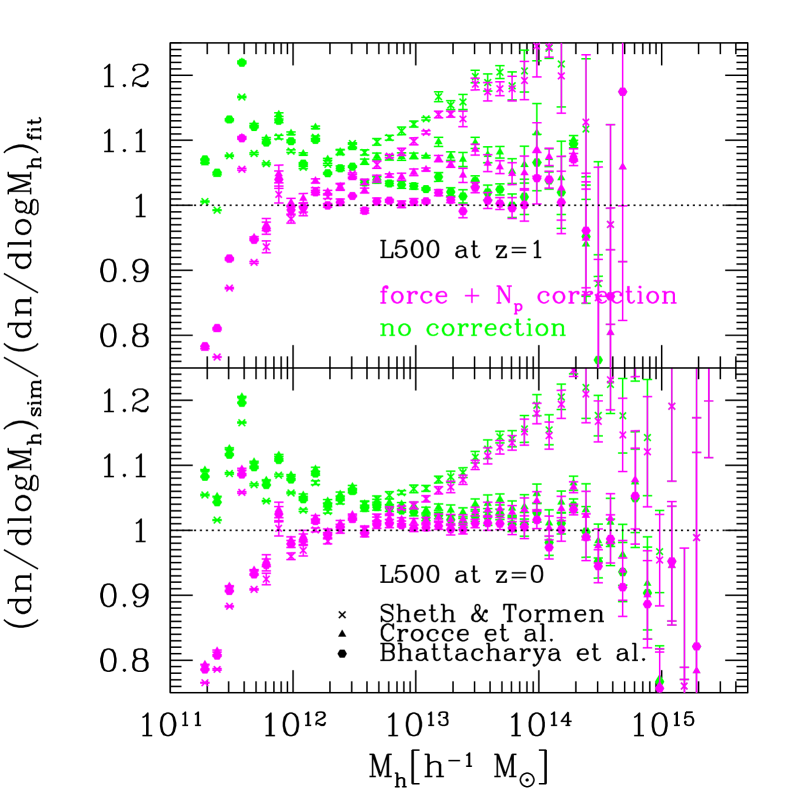
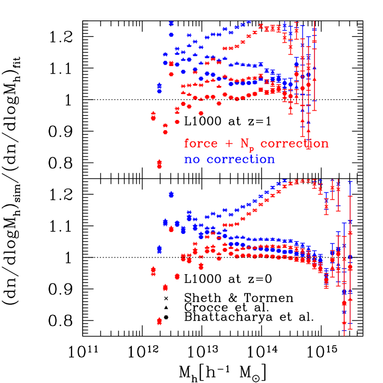
In Figure 4, to investigate the agreement in more quantitative ways, we show the ratio of the halo mass function obtained from $N$-body simulations to that from fitting formulae of Coyote and ST used in Figure 3. In addition to the above two fitting formulae, we use the recently proposed fitting formula by MICE. The left and right panels show the results of L500 and L1000 at $z=0$ and 1. We can see good agreement between our simulation results and the Coyote fitting formula within a few percent if we apply the correction (Eq. 29) to FOF halo masses. Also, the MICE fitting formula reproduces the simulation results applying FOF mass correction with the same level in Coyote at $z=0$, although the result at $z=1$ deviates about 5$\%$ from our simulation result. Meanwhile, ST results underpredict the simulation results by about 10$\%$-20$\%$ at $M_{h}>10^{13}h^{-1}M_{\odot}$. Therefore, the halo mass function obtained from our $N$-body simulations supports recently proposed fitting formulae obtained by using large and high-resolution $N$-body simulations and vice versa.

However, a closer look at $M_{h}<10^{12}h^{-1}M_{\odot}$ in the left panel and $M_{h}<10^{13}h^{-1}M_{\odot}$ in the right panel reveals deviation from unity which shows that the FOF correction may not be perfect in halos with small particles. Therefore, an accurate mass estimation requires keeping many more particles within individual halos, although halos with only a small number of particles ($\sim 20$) can be found using the FOF algorithm. Or a more accurate FOF mass correction needs to be developed. In addition, aside from simple considerations of particle shot noise, there is an inherent systematic error and scatter in the definition of a FOF halo mass with particle number, as pointed out by Warren et al. (2006).

Figure 5: The same as Figure 4, but Crocce et al. (2010) results are not plotted and the upper and bottom panels show the results at redshift 3 and 2.

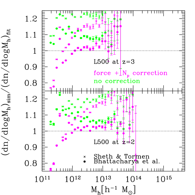
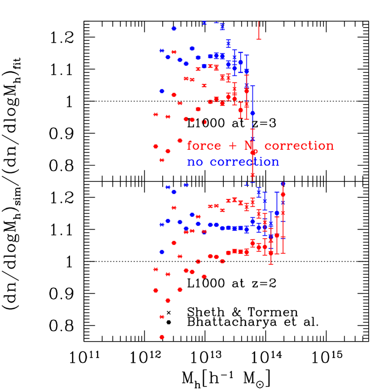
Figure 5 is the same as Figure 4, but at redshift 2 and 3 and results of the MICE fitting formula are not plotted because their fitting formula was fitted in the redshift range $z=0-1$. As in the results at $z=0$ and 1, our results are in good agreement with the Coyote results, although the application of their fitting formula to the result at $z=3$ might not be reliable, because the Coyote fitting formula was fitted between $z=0$ and $z=2$. As shown in Figure 4, the deviation from unity at low mass halos is also shown in Figure 5.

IV.4 Halo Biases

Figure 6: Comparison of halo power spectra obtained from $N$-body simulations to analytical predictions in real (left panel) and redshift (right panel) space for redshifts, $z=3$, 2, 1, and 0.5. Halo power spectra are normalized by the no-wiggle fitting formula $P_{\rm nw}(k)$ (Eisenstein and Hu, 1998) in real space and by the no-wiggle fitting formula taking the Kaiser effect into account $P^{s}_{\rm nw}(k)$ in redshift space, respectively. Therefore, the vertical axis shows the square of the halo bias. The solid and dotted curves show the predictions of the 1-loop Lagrangian resummation theory and linear theory, respectively. An enhancement of amplitude on small scales is due to the nonlinear effects of dynamics, bias, and redshift-space distortions.

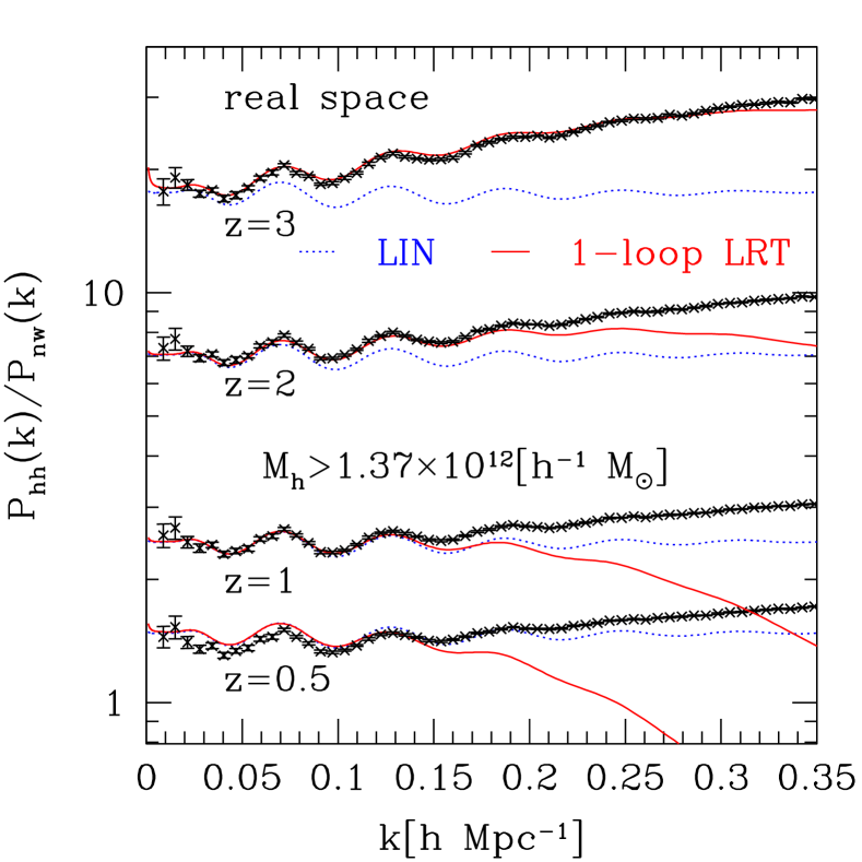
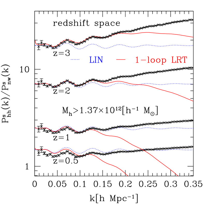
In Figure 6 we compare the halo power spectra computed from $N$-body simulations with the analytical predictions in real (left panel) and redshift (right panel) space for $z=3$, 2, 1, and 0.5. Halo power spectra are normalized by the no-wiggle fitting formula $P_{\rm nw}(k)$ (Eisenstein and Hu, 1998) in real space and by the no-wiggle fitting formula taking the Kaiser effect into account $P^{s}_{\rm nw}(k)$ in redshift space, respectively. In the monopole power spectrum we have considered, Kaiser’s enhancement effect $R_{\rm hh}$ is expressed as

$$R_{\rm hh}=1+\frac{2}{3}\beta+\frac{1}{5}\beta^{2},$$ (31)

from an angular average of the factor $(1+\beta\mu^{2})^{2}$ in Eq. (19). Therefore the vertical axis corresponds to the square of the halo bias, i.e., $b^{2}(k)$. The solid and dotted curves show the predictions of 1-loop LRT (Eqs. 9 and 14) and LIN (Eqs. 16 and 19), respectively. When we calculate the prediction of the 1-loop LRT, we use the Coyote fit (Eq. 28) for the halo mass function because the prediction of the Coyote fit is well duplicated by our simulation results as seen in Figures 4 and 5.

As increasing redshift, the amplitude of power spectrum becomes larger because we impose the same halo mass threshold ($M_{\rm h}>1.37\times 10^{12}h^{-1}M_{\odot}$) regardless of redshift. Halos which have a certain mass, for example, this threshold mass $M_{\rm h}>1.37\times 10^{12}h^{-1}M_{\odot}$, are increasingly rare as increasing redshift, and thus the amplitude of the power spectrum is more biased. Theoretical predictions of 1-loop LRT and LIN well agree with $N$-body simulations at large scales up to a certain scales. As in the matter power spectrum, the range of agreement in the 1-loop LRT prediction is wider as redshift is higher. Meanwhile the LIN prediction significantly deviates from the $N$-body results as bias is higher. Therefore, the 1-loop LRT prediction which include higher-order bias term is very powerful for future high redshift BAO surveys to extract the cosmological information. At very large scales if the mass function prediction is accurate, 1-loop LRT and LIN predictions should reproduce the simulation result because all the higher-order Lagrangian bias factors $\langle{F^{(n)}}\rangle$ should be zero except for $\langle{F^{\prime}}\rangle$. However, a closer look at small wave number $k$ for $z=0.5$ reveals a discrepancy in overall amplitudes between theoretical predictions and simulation results beyond the range of error bars. This might be ascribed to the fact that the FOF mass correction (Eq. 29) is not perfect in halos with small particles as shown in Figures 4 and 5.

Figure 7: The same as Figure 6, but the vertical axis is divided by $b^{2}=(1+\langle{F^{\prime}}\rangle)^{2}$ and $b^{2}R_{\rm hh}=(1+\langle{F^{\prime}}\rangle)^{2}(1+2\beta/3+\beta^{2}/5)$ in real and redshift space, respectively. An enhancement of amplitude on small scales comes from the nonlinear effects of dynamics, bias, and redshift-space distortions.

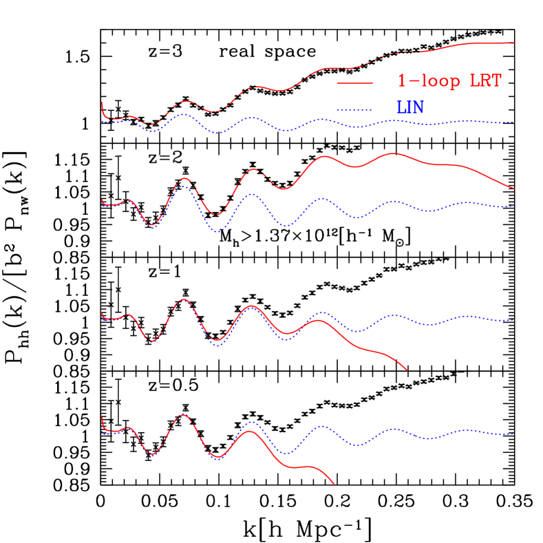
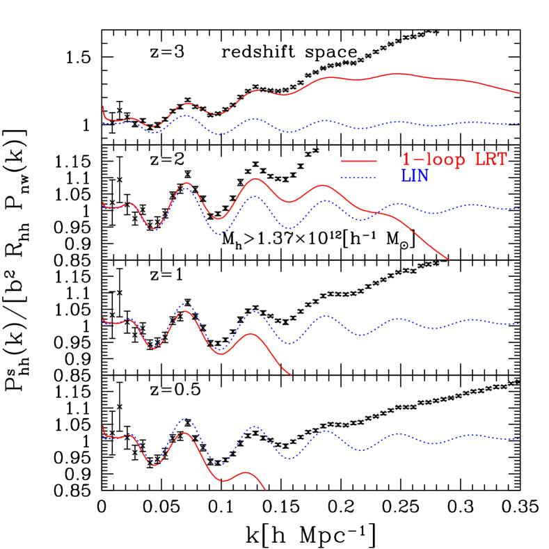
In Figure 7, to examine the agreement in more quantitative ways and exclude an uncertainty in amplitudes explained above, we eliminate dependences on the linear bias factor and linear Kaiser’s factor, dividing the power spectra by $b^{2}=(1+\langle{F^{\prime}}\rangle)^{2}$ and $b^{2}R_{\rm hh}=(1+\langle{F^{\prime}}\rangle)^{2}(1+2\beta/3+\beta^{2}/5)$ in real and redshift space, respectively. For simulation results $b^{2}$ and $b^{2}R_{\rm hh}$ are numerically estimated as follows. First, those factors can be computed among 30 realizations through

$$b^{2}(k)=\frac{P_{\rm hh}(k)}{P_{\rm mm}(k)},\qquad b^{2}(k)R_{\rm hh}=\frac{P_{\rm hh}^{\rm s}(k)}{P_{\rm mm}(k)},$$ (32)

where $P_{\rm mm}(k)$ denotes the real-space power spectrum of matter, and $P_{\rm hh}(k)$ and $P_{\rm hh}^{\rm s}(k)$ denote the halo power spectrum in real and redshift space. Those power spectra are obtained from $N$-body simulations. Second, we use polynomial fitting with

$$b^{2}(k) =A_{0}+\sum_{i=1}^{3}A_{i}k^{i},$$ (33)

$$b^{2}(k)R_{\rm hh} =B_{0}+\sum_{i=1}^{3}B_{i}k^{i}.$$ (34)

Finally, computing the $\chi^{2}$ statistics with the data up to $k$=0.35$h$Mpc^-1, we can obtain the best-fit values of scale independent terms, $A_{0}$ and $B_{0}$, and then we substitute these values into $b^{2}$ and $b^{2}R_{\rm hh}$, respectively.

Comparing the matter power spectra in Figure 1 and halo power spectra in Figure 7, the ranges of agreement between $N$-body simulations and 1-loop LRT predictions with halo bias seem to be the same as those in the matter power spectrum for all redshift we have examined in real space. However, the results of the halo power spectrum in redshift space seem to be somewhat worse than those of matter power spectrum as decreasing redshift. This might be because the effects of nonlinear redshift-space distortions become larger as decreasing redshift. The redshift-space distortion parameter $\beta\simeq\Omega_{m}^{0.55}/b$ becomes larger as decreasing redshift since a halos at lower redshift are less biased than those at higher redshift. Therefore, 1-loop LRT well replicate the $N$-body simulation results on BAO scales even in existence of halo bias, although the results of low redshifts in redshift space are less accurately reproduced by 1-loop LRT. Comparing the results of real space at $z=0.5$ and $z=1$ in Figure 1 and those in Figure 7, an enhancement of amplitude of halo power spectra on small scales is slightly moderate because $\langle{F^{\prime\prime}}\rangle$ has a negative value, which is calculated from Eq. (10), where we substitute the minimum halo mass in our simulations, $M_{\rm h}=1.37\times 10^{12}h^{-1}M_{\odot}$, into $M_{1}$ and infinity into $M_{2}$. In contrast, other redshift results ($z=2$ and 3) of halos in real space are more enhanced compared to those of matter power spectrum, since $\langle{F^{\prime\prime}}\rangle$ has a positive value at $z=2$ and 3. In redshift space, amplitudes of the results of halo power spectrum are enhanced compared to those of matter power spectrum at all redshift. This is due to the nonlinear effects of bias and redshift-space distortions. This scale dependence of bias coming from the clustering of halos and nonlinear redshift-space distortions will be carefully examined in Figure 8.

Figure 8: The same as Figure 7, but the smooth linear power spectrum $P_{\rm nw}(k)$ is replaced with $P_{\rm mm}(k)$ and $P_{\rm mm}^{\rm s}(k)/R_{\rm mm}$ in real and redshift space, respectively in order to get rid of the nonlinearity of dynamics. Therefore deviation from unity shows the nonlinearity of bias and that of bias and redshift-space distortions in real and redshift space. $P_{\rm mm}(k)$ and $P_{\rm mm}^{\rm s}(k)$ are corresponding mass power spectra in real and redshift space. $R_{\rm mm}$ is Kaiser’s enhancement factor of matter defined by $R_{\rm mm}=1+2f/3+f^{2}/5$.

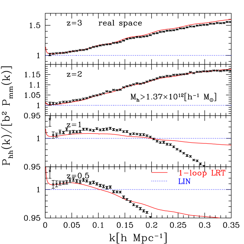
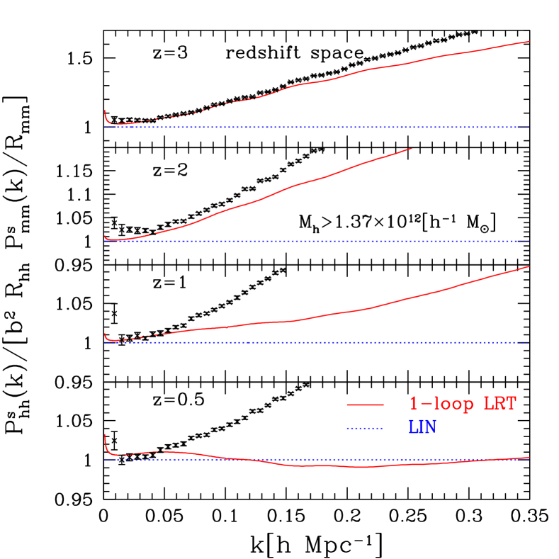
Figure 8 is the same as Figure 7, but the smooth no-wiggle linear power spectrum $P_{\rm nw}(k)$ is replaced with $P_{\rm mm}(k)$ and $P_{\rm mm}^{\rm s}(k)/R_{\rm mm}$ in real and redshift space, respectively. Here $P_{\rm mm}(k)$ and $P_{\rm mm}^{\rm s}(k)$ are corresponding mass power spectra in real and redshift space. $R_{\rm mm}$ is Kaiser’s enhancement factor of matter, which is obtained from Eq. (31) with $b=1$ as

$$R_{\rm mm}=1+\frac{2}{3}f+\frac{1}{5}f^{2}.$$ (35)

For simulation results in redshift space, $b^{2}R_{\rm hh}/R_{\rm mm}$ is estimated from simulations through

$$b^{2}(k)R_{\rm hh}/R_{\rm mm}=\frac{P_{\rm hh}^{\rm s}(k)}{P_{\rm mm}^{\rm s}(k)}.$$ (36)

Using polynomial fitting with

$$b^{2}(k)R_{\rm hh}/R_{\rm mm}=C_{0}+\sum_{i=1}^{3}C_{i}k^{i},$$ (37)

we calculate the $\chi^{2}$ statistics with the data up to $k$=0.35$h$Mpc^-1 and search for the best-fit value of scale independent term, $C_{0}$. Then, we substitute the best-fit value into $b^{2}R_{\rm hh}/R_{\rm mm}$.

The functional form of vertical axis in real space, $P_{\rm hh}(k)/[b^{2}P_{\rm mm}(k)]$, describes only the nonlinear effect of bias, so a deviation from unity shows the scale dependence of bias. Meanwhile in redshift space the vertical axis shows nonlinear effects of bias and redshift-space distortions. We find that the scale dependence of bias does not show significant oscillations and are mostly smooth functions of scales. The scale dependence and nonlinearity of bias shown in our results purely originate from clustering of halos themselves. LIN predicts constancy of halo bias on all scales. We find that scale dependences of bias calculated from our simulation results are in fairly good agreement with 1-loop LRT predictions up to $k=0.35h$Mpc^-1 ($z=2$ and 3) within a few percent level and up to $k=0.1h$ Mpc^-1 ($z=2$) and 0.15$h$Mpc^-1 ($z=3$) in redshift space. Recent analytical and numerical studies claim that the scale-dependent and stochastic properties of the bias can change the redshift-space power spectrum and those impacts on the determination of the growth-rate parameter would be significant (Jeong and Komatsu, 2009; Desjacques and Sheth, 2010; Jennings et al., 2011; Okumura and Jing, 2011; Saito et al., 2011). Therefore LRT prediction is useful and powerful to model biasing relevant for BAO scales.

Figure 9: Comparison of halo two-point correlation functions computed from $N$-body simulations to analytical predictions in real (left panel) and redshift (right panel) space for redshifts, $z=3$, 2, 1, 0.5 and 0 from bottom to top. Halo correlation functions are normalized by $b^{2}=(1+\langle{F^{\prime}}\rangle)^{2}$ and $b^{2}R_{\rm hh}=(1+\langle{F^{\prime}}\rangle)^{2}(1+2\beta/3+\beta^{2}/5)$ in real and redshift space, respectively. The solid curves represent the results of the 1-loop Lagrangian resummation theory while the dotted curves show the results of the linear theory.

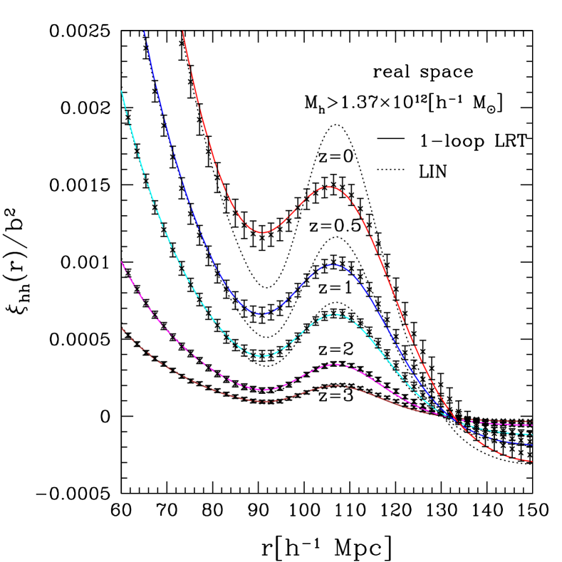
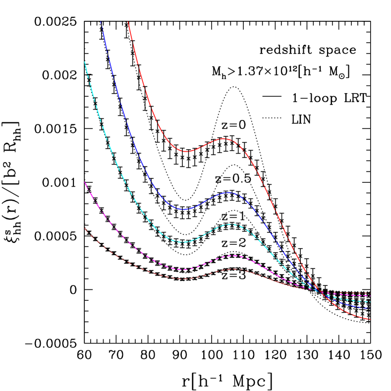
Finally, we examine the two-point correlation function of halos for $z=3$, 2, 1, 0.5, and 0 both in real and redshift space, shown in the left and right panels of Figure 9, respectively. Two-point correlation functions of halos are divided by $b^{2}=(1+\langle{F^{\prime}}\rangle)^{2}$ and $b^{2}R_{\rm hh}=(1+\langle{F^{\prime}}\rangle)^{2}(1+2\beta/3+\beta^{2}/5)$ in real and redshift space, respectively. The solid curves represent the results of 1-loop LRT while the dotted curves show the results of LIN. For simulation results $b^{2}$ and $b^{2}R_{\rm hh}$ are fitted in the same manner as in the case of the halo power spectrum (Figures 7 and 8). Those can be calculated among 30 realizations through

$$b^{2}(r)=\frac{\xi_{\rm hh}(r)}{\xi_{\rm mm}(r)},\qquad b^{2}(r)R_{\rm hh}=\frac{\xi_{\rm hh}^{\rm s}(r)}{\xi_{\rm mm}(r)},$$ (38)

where $\xi_{\rm mm}(r)$ denotes the matter correlation function in real space, and $\xi_{\rm hh}(r)$ and $\xi_{\rm hh}^{\rm s}(r)$ denote the halo correlation functions in real and redshift space. Those correlation functions are obtained from $N$-body simulations. We assume $b^{2}(r)$ and $b^{2}(r)R_{\rm hh}$ to be constant on sufficiently large scales both in real and redshift space and chose $30h^{-1}$Mpc $<r<80h^{-1}$Mpc in configuration space. Then we compute $\chi^{2}$ for the above range to obtain $b^{2}$ and $b^{2}R_{\rm hh}$.

The left panel in Figure 9 is quite similar to the left panel in Figure 2. This shows that halo bias does not significantly change the shape of BAOs peak and that the effects of nonlinear halo bias are not significantly relevant for BAO scales in the correlation function. This result is consistent with a recent analysis of halo clustering by using numerical simulations (Sánchez et al., 2008). By comparing the left and right panels in Figure 9, we can see the nonlinear effect of redshift-space distortions. It smears the BAO peaks and troughs as decreasing the redshift. One-loop LRT with halo bias shows good agreement with $N$-body simulation results and well captures the features of nonlinear effects as in the matter correlation function. The results of 1-loop LRT in redshift space slightly deviate from those of simulations at low redshifts. This should be related to the inaccuracy of the 1-loop LRT in the low-redshift power spectra as seen in Figure 7.

V Conclusion

To exploit the full potential of upcoming high-quality data, we have to precisely describe observable features of BAOs. To achieve this purpose, taking account of the galaxy biasing and redshift-space distortions is essential. In this paper, we have used 30 large cosmological $N$-body simulations of the standard $\Lambda$CDM cosmology to investigate the halo biases over a wide redshift range.

First, in the matter power spectrum, 1-loop LRT is useful for studying nonlinear effects on scales of BAOs and provides better agreement with $N$-body results than 1-loop SPT or the prediction of Scoccimarro (2004) on large scales in observable redshift space. Second, in the matter correlation function, 1-loop LRT prediction well describes the acoustic peaks and nonlinear smearing effects both in real and redshift space. The 2-loop correction to LRT generally extends the valid range in the matter power spectrum. It does not have much impact on the correlation function in real space, because 1-loop LRT is already accurate enough to describe the nonlinear effects on BAO scales in $N$-body simulations (Okamura et al., 2011). However, the predictions of 1-loop LRT for low-redshift correlation functions in redshift space would be improved if the 2-loop corrections are included.

In the halo power spectrum, we found that 1-loop LRT prediction has good agreement with $N$-body simulation results. The ranges of agreement seem the same as those in the matter power spectrum for all redshift in real space. In redshift space, the 1-loop LRT prediction for the halo power spectrum is slightly worse than that for the matter power spectrum. This might be because the nonlinear effects of redshift-space distortions become larger as decreasing the redshift. This shows that the 1-loop LRT prediction well reproduces the $N$-body simulation results on BAO scales even in the existence of halo bias at least in real space. We found that the scale dependences of bias are pretty well reproduced by 1-loop LRT up to $k=0.35h$Mpc^-1 ($z=2$ and 3) within a few percent level in real space and up to $k=0.1h$Mpc^-1 ($z=2$) and 0.15$h$Mpc^-1 ($z=$3) in redshift space. In the halo correlation function, 1-loop LRT well describes nonlinear effects that smear the baryon peak and trough both in real and redshift space. Halo bias does not significantly change the shape of the baryon peak. Therefore, the nonlinear effects of halo bias are not serious on BAO scales.

Thus, LRT prediction is very powerful and reliable to accurately extract cosmological information for upcoming high redshift BAO surveys.